1. Introduction
It is hard to name any other branch of oceanography that would enjoy such persistent interest and broad acceptance of its significance but, at the same time, would remain as underexplored as the flow-topography interaction theory. Particularly nascent is our understanding of processes induced by the sea-floor roughness, defined here as bathymetric features with a lateral extent of several kilometres. Rough topography affects several aspects of ocean circulation. It tends to suppress baroclinic instability, thereby controlling the intensity of mesoscale variability in the ocean (LaCasce et al. Reference LaCasce, Escartin, Chassignet and Xu2019; Radko Reference Radko2020). Sea-floor roughness extends the lifespan of coherent vortices (Gulliver & Radko Reference Gulliver and Radko2022), enhancing their ability to transport heat, salt, and nutrients. On a more conceptual level, rough topography could be the key to one of the most fundamental problems in geophysical fluid dynamics, the explanation of the direct cascade of energy and thermal variance. Mechanical and thermodynamic forcing at the sea surface occurs on the scales of ocean basins, whereas the energy and thermal variance are ultimately dissipated by molecular processes acting on the microscale (Wunsch & Ferrari Reference Wunsch and Ferrari2004; Merryfield Reference Merryfield2005). The small-scale eddies generated by rough topography could dynamically connect microstructure with larger scales of motion (Dewar & Hogg Reference Dewar and Hogg2010; Dewar, Berloff, & Hogg Reference Dewar, Berloff and Hogg2011) and, therefore, investigations of flow-topography interactions may lead to essential insights into global energetics.
While there is little doubt about the overall importance of sea-floor roughness, a consistent view of the specific mechanisms at play – and their relative impact on large-scale patterns – is only beginning to emerge. Traditionally, much attention has been paid to the effects of topographic pressure torque (Hughes & de Cuevas Reference Hughes and De Cuevas2001; Jackson, Hughes, & Williams Reference Jackson, Hughes and Williams2006; Stewart, McWilliams, & Solodoch Reference Stewart, McWilliams and Solodoch2021), with particular emphasis on lee-wave drag (Naveira Garabato et al. Reference Naveira Garabato, Nurser, Scott and Goff2013; Eden, Olbers, & Eriksen Reference Eden, Olbers and Eriksen2021; Klymak et al. Reference Klymak, Balwada, Garabato and Abernathey2021). Several observable phenomena are caused by the topographic steering of low Rossby number flows (Marshall Reference Marshall1995; Wåhlin Reference Wåhlin2002). It is manifested, for instance, in the formation of stationary Taylor columns that trap fluid above salient topographic features (Taylor Reference Taylor1923; Johnson Reference Johnson1978). Yet another distinct mechanism of topographic control involves small-scale eddies generated by large-scale currents interacting with rough bathymetry. These eddies produce Reynolds stresses that, in turn, influence primary flows. Several examples of such dynamics were presented by Holloway (Reference Holloway1987, Reference Holloway1992), who argued that the interaction between topography and eddies can, in some cases, reinforce primary circulation patterns. In other systems, the topographic eddy stresses tend to substantially slow down abyssal currents (Radko Reference Radko2020; Gulliver & Radko Reference Gulliver and Radko2022).
One of the key objectives of the flow-topography interaction theory is the development of explicit closure models representing the impact of sea-floor roughness on large-scale flows. The pragmatic motivation for this effort is related to the resolution limitations of general circulation models. Despite advancements in high-performance computing, roughness-resolving global models will not be used for extended climate simulations in the foreseeable future. Thus, parameterizing the effects of small-scale bathymetry is the most promising way forward. Adopting topographic closure models also enhances the prospects of finding analytical solutions that conceptualize large-scale oceanic phenomena affected by sea-floor roughness. Finally, as our study illustrates, the very process of developing such parameterizations can be highly effective in terms of explaining the essential dynamics at work.
In the present investigation, closure models for sea-floor roughness are developed using techniques of multiscale analysis, a broad and active field with numerous fluid-dynamical applications (e.g. Meshalkin & Sinai Reference Meshalkin and Sinai1961; Manfroi & Young Reference Manfroi and Young1999, Reference Manfroi and Young2002; Balmforth & Young, Reference Balmforth and Young2002, Reference Balmforth and Young2005; Mei & Vernescu Reference Mei and Vernescu2010). The principal idea of multiscale methods involves rewriting the governing equations using two sets of independent variables. In our case, large scales describe primary flows, and small ones are based on the lateral extent of topographic features that the model strives to parameterize. The crux of this approach is the derivation of solvability conditions that describe the system entirely on large scales. Strictly speaking, the theory assumes scale separation between the primary flow components and those induced by rough topography. It is unclear how well this assumption describes nature, but we assume and subsequently verify that the resulting analytical model reflects behaviours that hold even without the scale separation. Our earlier results in this area (e.g. Radko & Kamenkovich Reference Radko and Kamenkovich2017; Radko Reference Radko2020, Reference Radko2022a,Reference Radkob) also indicate that multiscale models perform remarkably well for a wide range of systems, including those in which the lines between large and small scales are blurred.
Traditionally, multiscale methods have been applied to simple analytical small-scale patterns (e.g. Gama, Vergassola, & Frisch Reference Gama, Vergassola and Frisch1994; Novikov & Papanicolau Reference Novikov and Papanicolau2001; Radko Reference Radko2011a,Reference Radkob), ultimately leading to explicit large-scale equations. In the context of flow-topography interaction problems, analytical progress has been made for one-dimensional sinusoidal bathymetry (e.g. Benilov Reference Benilov2000, Reference Benilov2001; Vanneste Reference Vanneste2003; Radko Reference Radko2020). The representation of more realistic irregular two-dimensional topographic features is more challenging and explicit solutions have mostly been derived for special cases (e.g. Vanneste Reference Vanneste2000; Goldsmith & Esler Reference Goldsmith and Esler2021). The fundamental limitation of such models is their inherently qualitative connection to the observed or simulated phenomena.
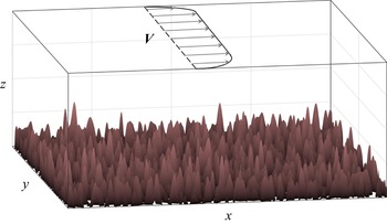
Fortunately, a recent advancement opened the path for analytical treatments of realistic patterns of small-scale topography. Radko (Reference Radko2022a,Reference Radkob) pointed out that multiscale methods can be effectively applied to irregular bathymetry, provided that its statistical spectral representation is known. The key step is the application of Parseval's theorem (Parseval Reference Parseval1806), equating the spatial average of any quadratic quantity to integrals of Fourier coefficients in wavenumber space. This link proved to be critical since ocean depth variability is adequately represented by the observationally derived spectrum of Goff & Jordan (Reference Goff and Jordan1988). The resulting framework was termed the sandpaper model, a nickname invoking associations with small, irregular, tightly packed particles of sandpaper – features that are reminiscent of rough bathymetry in the ocean (figure 1). The sandpaper model has led to an explicit representation of flow forcing by rough topography, essentially yielding a rigorous asymptotics-based parameterization.
Schematic diagram illustrating the set-up of the sandpaper model. A large-scale flow interacts with irregular sea floor, the pattern of which conforms to the Goff & Jordan (Reference Goff and Jordan1988) spectrum.

The previous versions of the sandpaper model (Radko Reference Radko2022a,Reference Radkob) were successfully tested for oceanographically relevant parameters on the canonical vortex spin-down problem. These works, however, have also raised several fundamental questions that the present investigation attempts to address. The primary concern is the generality of the proposed solutions. The models of Radko (Reference Radko2022a,Reference Radkob) explored a specific sector in the multidimensional parameter space characterized by rapid flows with asymptotically large Reynolds numbers. However, there are clear signs that the solutions obtained for this regime are not universal. For instance, the expressions for topographic forcing derived by Radko (Reference Radko2022a,Reference Radkob) are inversely proportional to large-scale velocity. This singularity suggests that forcing unphysically increases without bound with decreasing flow speed – a tell-tale sign that a different asymptotic model is needed to capture the limit of weak large-scale currents.
To explore a wider range of parameters and ultimately develop a general model of topographic forcing, we consider an asymptotic sector corresponding to slow flows with low Reynolds numbers. The properties of fast- and slow-flow models turned out to be fundamentally different. For instance, the fast-flow regime (Radko, Reference Radko2022a,Reference Radkob) is characterized by the profound influence of the Reynolds stresses produced by the interaction of large-scale currents with rough bathymetry. Slow currents, on the other hand, are controlled by the eddy-induced form drag, and in this limit, the large-scale forcing by rough topography is proportional to large-scale velocity. To offer a more universal description of the flow field, we propose a hybrid closure for sea-floor roughness that converges to the corresponding asymptotic expressions in the limits of fast and slow currents. In contrast to the earlier parameterizations of Radko (Reference Radko2022a,Reference Radkob), which required an ad hoc regularization for weak large-scale flows, the hybrid model is well behaved and can be readily implemented in large-scale evolutionary equations.
The material is organized as follows. The governing equations for the homogeneous model are described in § 2. Section 3 presents the asymptotic multiscale theory that leads to an explicit closure for small-scale bathymetry. The analytical model is validated by roughness-resolving simulations in § 4. The extension of the asymptotic analysis to the multilayer framework is discussed in § 5. The results are summarized, and conclusions are drawn, in § 6.
2. The homogeneous model
Our starting point is the homogeneous quasi-geostrophic rigid-lid model (e.g. Pedlosky Reference Pedlosky1987)
 \begin{equation}\frac{{\partial {\nabla ^2}{\psi ^ \ast }}}{{\partial {t^\ast }}} + J({\psi ^\ast },{\nabla ^2}{\psi ^\ast }) + {\beta ^\ast }\frac{{\partial {\psi ^\ast }}}{{\partial {x^\ast }}} + \frac{{f_0^\ast }}{{H_0^\ast }}J({\psi ^\ast },{\eta ^\ast }) = {\nu ^\ast }{\nabla ^4}{\psi ^\ast } - {\gamma ^\ast }{\nabla ^2}{\psi ^\ast },\end{equation}
where  ${\psi ^\ast }$ is the streamfunction associated with the velocity field
 $({u^\ast },{v^\ast }) = ( - \partial {\psi ^\ast }/\partial {y^\ast },\partial {\psi ^\ast }/\partial {x^\ast })$,
 ${\eta ^\ast }$ is the depth variation, J is the Jacobian,
 ${\nu ^\ast }$ is the lateral eddy viscosity and
 ${\gamma ^\ast }$ is the Ekman bottom drag coefficient. Also,
 $H_0^\ast $ and
 $f_0^\ast $ are the reference values of the ocean depth and the Coriolis parameters, respectively, and
 ${\beta ^\ast } \equiv \partial {f^\ast }/\partial {y^\ast }$ is the meridional gradient of planetary vorticity. The asterisks represent dimensional quantities.
We explore the impact of topographic patterns with the lateral extent  $O({L^\ast })$ on large-scale flows with scales
 $O(L_{LS}^\ast )$. We assume that fine topographic scales are limited to a finite range
 $[L_{min}^\ast ,L_C^\ast ]$, where
 $L_C^\ast $ is the cutoff wavelength formally separating small and large scales. The lower bound
 $(L_{min}^\ast )$ is introduced to ensure that all relevant Rossby numbers are low – the key assumption of the quasi-geostrophic framework. This leads to the following ordering of spatial scales:
 \begin{equation}\frac{{{U^\ast }}}{{f_0^\ast }} \ll L_{min}^\ast < {L^\ast } < L_C^\ast\ll L_{LS}^\ast ,\end{equation}
where  ${U^\ast }$ is the velocity scale. The number of controlling parameters is reduced by non-dimensionalizing (2.1) using
 $1/f_0^\ast $ and
 ${L^\ast }$ as the units of time and lateral extent, respectively,
 \begin{equation}{\psi ^\ast } = f_0^\ast {L^{{\ast} 2}}\psi ,\quad {x^\ast } = {L^\ast }x,\quad {y^\ast } = {L^\ast }y,\quad {t^\ast } = \frac{t}{{f_0^\ast }}.\end{equation}
The topographic height, however, is non-dimensionalized as
 \begin{equation}{\eta ^\ast } = H_0^\ast \eta .\end{equation}
To be specific, we consider the oceanographically relevant scales of
 \begin{equation}{L^\ast } = {10^4}\ \textrm{m},\quad H_0^\ast= 4000\ \textrm{m},\quad f_0^\ast= {10^{ - 4}}\ \textrm{s}{}^{ - 1}.\end{equation}
The non-dimensionalization reduces the governing equation (2.1) to
 \begin{equation}\frac{{\partial {\nabla ^2}\psi }}{{\partial t}} + J(\psi ,{\nabla ^2}\psi ) + \beta \frac{{\partial \psi }}{{\partial x}} + J(\psi ,\eta ) = \nu {\nabla ^4}\psi - \gamma {\nabla ^2}\psi ,\end{equation}
where
 \begin{equation}\beta = \frac{{{\beta ^\ast }{L^\ast }}}{{f_0^\ast }},\quad \nu = \frac{{{\nu ^\ast }}}{{f_0^\ast {L^{{\ast} 2}}}},\quad \gamma = \frac{{{\gamma ^\ast }}}{{f_0^\ast }}.\end{equation}
To explore the interaction between flow components of large and small lateral extents, we introduce the scale-separation parameter
 \begin{equation}\varepsilon = \frac{{L_C^\ast }}{{L_{LS}^\ast }} \ll 1.\end{equation}
This parameter is used to define the new set of spatial scales  $(X,Y)$ that reflect the dynamics of large-scale processes. These variables are related to the original ones through
 \begin{equation}(X,Y) = \varepsilon (x,y).\end{equation}
The derivatives in the governing system (2.6) are replaced accordingly
 \begin{equation}\frac{\partial }{{\partial x}} \to \frac{\partial }{{\partial x}} + \varepsilon \frac{\partial }{{\partial X}},\quad \frac{\partial }{{\partial y}} \to \frac{\partial }{{\partial y}} + \varepsilon \frac{\partial }{{\partial Y}}.\end{equation}
Topographic patterns considered in the sandpaper model vary on both large and small scales
 \begin{equation}\eta = {\eta _L}(X,Y) + {\eta _S}(x,y).\end{equation}
A natural way to separate bathymetry into the small- and large-scale components (Radko Reference Radko2022a,Reference Radkob) is based on the Fourier transform of  $\eta $
 \begin{equation}\eta = \frac{{\sqrt {{L_x}{L_y}} }}{{2{\rm \pi} }}\iint {\tilde{\eta }(k,l)\,\textrm{exp}(\textrm{i}kx + \textrm{i}ly)\,\textrm{d}k\,\textrm{d}l} ,\end{equation}
where  $(k,l)$ are the wavenumbers in x and y, respectively, tildes hereafter denote Fourier images and
 $({L_x},{L_y})$ is the domain size. Since the Fourier transform is linear, it can be conveniently separated into the contributions from high and low wavenumbers as follows:
 \begin{equation}\begin{array}{ccccc} \eta & =\underbrace{{\dfrac{{\sqrt {{L_x}{L_y}} }}{{2{\rm \pi} }}\iint_{\kappa < 2{\rm \pi} /{L_C}} {\tilde{\eta }(k,l)\,\textrm{exp}(\textrm{i}kx + \textrm{i}ly)\,\textrm{d}k\,\textrm{d}l} }}_{{{\eta _L}}}\\ & + \underbrace{{\dfrac{{\sqrt {{L_x}{L_y}} }}{{2{\rm \pi} }}\iint_{\kappa > 2{\rm \pi} /{L_C}} {\tilde{\eta }(k,l)\,\textrm{exp}(\textrm{i}kx + \textrm{i}ly)\,\textrm{d}k\,\textrm{d}l} }}_{{{\eta _S}}}, \end{array}\end{equation}
where  $\kappa \equiv \sqrt {{k^2} + {l^2}} $. The
 ${\eta _L}$ component in (2.13) gently varies on large scales, and
 ${\eta _L}$ represents small-scale variability. The normalization factor
 $\sqrt {{L_x}{L_y}} /2{\rm \pi} $ in the definition of the Fourier transform is introduced to ensure that the Parseval identity (Parseval 1806), to be used in subsequent developments, takes a convenient form
 \begin{equation}{\langle ab\rangle _{x,y}} = \iint {\tilde{a} \cdot \textrm{conj}(\tilde{b})\,\textrm{d}k\,\textrm{d}l.}\end{equation}
Angle brackets hereafter represent mean values, with the averaging variables listed in the subscript.
3. The multiscale analysis
We now explore flow-topography interactions using methods of multiscale mechanics. Our earlier efforts in this area (Radko Reference Radko2022a,Reference Radkob) have led to a consistent treatment of relatively swift flows. However, the resulting theory was inapplicable for weak currents, motivating the development of an analogous slow-flow model. To highlight the principal differences and similarities between the two systems, we first review the key features of the fast-flow model.
3.1. Rapid flows
The barotropic sandpaper theory (Radko, Reference Radko2022a) was based on the expansion in small parameter  $\varepsilon $quantifying the disparity of large and small spatial scales (2.8). The flow was assumed to be inviscid at the leading order with
 \begin{equation}Re = \frac{{{U^\ast }{L^\ast }}}{{{\nu ^\ast }}} = O({\varepsilon ^{ - 1}}).\end{equation}
Nevertheless, even weak friction proved to be critical due to the catalytic nature of rough topography, which amplified the effects of explicit dissipation by as much as 2–3 orders of magnitude. The expansion opened with a large-scale flow  $\bar{\psi }(X,Y,t)$ and its first-order correction was represented by a small-scale pattern
 ${\psi _S}(x,y)$. The dynamics of this perturbation was controlled by the homogenization of small-scale potential vorticity (PV), with
 ${\psi _S}$ rigidly controlled by topography and satisfying
 \begin{equation}{\nabla ^2}{\psi _S} + {\eta _S}(x,y) = 0.\end{equation}
The closed evolutionary equation for  $\bar{\psi }$ was obtained as a solvability condition by averaging the governing equation in small-scale variables. In terms of original variables (2.9), the
 $\bar{\psi }$ equation takes the form
 \begin{equation}\frac{\partial }{{\partial t}}{\nabla ^2}\bar{\psi } + J(\bar{\psi },{\nabla ^2}\bar{\psi } + {\eta _L}) + \beta \frac{{\partial \bar{\psi }}}{{\partial x}} + {D_{fast}} + \gamma {\nabla ^2}\bar{\psi } = \nu {\nabla ^4}\bar{\psi },\end{equation}
where  ${D_{fast}}$ represents cumulative effects of rough bathymetry. It originates from the averaged nonlinear advective term
 ${\langle J(\psi ^{\prime},{\nabla ^2}\psi ^{\prime})\rangle _{x,y}}$ in the governing vorticity equation, where
 $\psi ^{\prime} = \psi - \bar{\psi }$, and represents the eddy-induced mixing of momentum. Interestingly, the topographic form drag does not affect the large-scale circulation at the leading order.
In this fast-flow regime, topographic forcing reduces to
 \begin{equation}{D_{fast}} = {G_{fast}}\left( {\frac{\partial }{{\partial x}}\left( {\frac{{\bar{v}}}{{{{\bar{u}}^2} + {{\bar{v}}^2}}}} \right) - \frac{\partial }{{\partial y}}\left( {\frac{{\bar{u}}}{{{{\bar{u}}^2} + {{\bar{v}}^2}}}} \right)} \right),\end{equation}
where  $(\bar{u},\bar{v}) = ( - \partial \bar{\psi }/\partial y,\partial \bar{\psi }/\partial x)$. The coefficient
 ${G_{fast}}$ in (3.4) is fully determined by the spectrum of small-scale topography and the explicit dissipation parameters
 \begin{equation}{G_{fast}} = 2{\rm \pi} \int {{{|{{{\tilde{\eta }}_S}} |}^2}\left( {\frac{\gamma }{\kappa } + \nu \kappa } \right)\textrm{d}\kappa } ,\quad \kappa = \sqrt {{k^2} + {l^2}} ,\end{equation}
where  ${\tilde{\eta }_S}$ is the Fourier image of the statistically isotropic small-scale component of topography. In essence, this theory parameterizes the effects of sea-floor roughness on larger scales of motion. However, the parameterization is derived directly from governing equations without invoking any empirical assumptions, commonly used by other closure models. The benefits brought by the sandpaper model include the opportunity to perform efficient numerical experiments without having to resolve small-scale features of the bottom relief if the spectrum of topography is known.
Unfortunately, there is one feature that seems unphysical and complicates the direct implementation of (3.3)–(3.5) in numerical models – the unbounded increase of (3.4) in the weak flow limit:  $\bar{V} \equiv \sqrt {{{\bar{u}}^2} + {{\bar{v}}^2}} \to 0$. Radko (Reference Radko2022a,Reference Radkob) has dealt with this inconvenience by constraining
 ${D_{fast}}$ in low-speed regions. While such regularization served the immediate purpose, making it possible to perform parametric simulations, its ad hoc character brought a certain sense of dissatisfaction. It implied that the model failed to capture the dynamics of weak flows, and the following analysis seeks to rectify this deficiency.
3.2. Weak flows
To offer an analogous description of the slow-flow limit, we now consider a regime in which Reynolds numbers are asymptotically small
 \begin{equation}Re = \frac{{{U^\ast }{L^\ast }}}{{{\nu ^\ast }}} = O(\varepsilon ).\end{equation}
This limit is captured by the expansion that opens with the  $O(\varepsilon )$ large-scale pattern
 \begin{equation}\bar{\psi } = \varepsilon {\psi ^{(1)}}(X,Y,T).\end{equation}
The governing parameters are rescaled as follows:
 \begin{equation}\beta = {\varepsilon ^4}{\beta _0},\quad \gamma = {\varepsilon ^3}{\gamma _0},\quad \nu = \varepsilon {\nu _0},\quad {\eta _S} = {\varepsilon ^2}{\eta _{S0}},\quad {\eta _L} = {\varepsilon ^3}{\eta _{L0}},\end{equation}
which affords the inclusion of all relevant effects in the evolutionary equation and broadly reflects the typical values of parameters in the oceanographic context. The temporal evolution in this regime is controlled by relatively slow processes driven by explicit dissipation. Hence, the temporal variable is rescaled as  $T = {\varepsilon ^3}t$, and the time derivative in the governing system (2.6) is replaced accordingly
 \begin{equation}\frac{\partial }{{\partial t}} \to {\varepsilon ^3}\frac{\partial }{{\partial T}}.\end{equation}
The interaction of the large-scale flow with low-amplitude rough topography forces the small-scale streamfunction response at  $O({\varepsilon ^3})$ and the asymptotic series are extended accordingly
 \begin{equation}\psi = \varepsilon {\psi ^{(1)}}(X,Y,T) + {\varepsilon ^3}{\psi ^{(3)}}(X,Y,x,y,T) + O({\varepsilon ^4}).\end{equation}
Series (3.10) are then substituted in the governing equation (2.6) and terms of the same order in  $\varepsilon $ are collected. The leading-order balance is realized at
 $O({\varepsilon ^4})$
 \begin{equation}\frac{{\partial {\psi ^{(1)}}}}{{\partial X}}\frac{{\partial {\eta _{S0}}}}{{\partial y}} - \frac{{\partial {\psi ^{(1)}}}}{{\partial Y}}\frac{{\partial {\eta _{S0}}}}{{\partial x}} = {\nu _0}{\nabla ^4}{\psi ^{(3)}}.\end{equation}
The  $O({\varepsilon ^5})$ balance plays no role in the model development and is not listed here. The key solvability condition leading to the evolutionary equation for
 $\bar{\psi }$ is obtained by averaging the
 $O({\varepsilon ^6})$ balance in
 $(x,y)$
 \begin{align}\frac{{\partial {\varsigma ^{(1)}}}}{{\partial T}} {\,+\,} {J_{X,Y}}({\psi ^{(1)}},{\varsigma ^{(1)}} {\,+\,} {\eta _{L0}}) {\,+\,} {\beta _0}\frac{{\partial {\psi ^{(1)}}}}{{\partial X}} {\,+\,} {D_{slow\ 0}} {\,+\,} {\gamma _0}{\varsigma ^{(1)}} = {\nu _0}\left( {\frac{{{\partial^2}{\varsigma^{(1)}}}}{{\partial {X^2}}} {\,+\,} \frac{{{\partial^2}{\varsigma^{(1)}}}}{{\partial {Y^2}}}} \right),\end{align}
where  ${\varsigma ^{(1)}} \equiv {\partial ^2}{\psi ^{(1)}}/\partial {X^2} + {\partial ^2}{\psi ^{(1)}}/\partial {Y^2}$ and
 \begin{equation}{D_{slow\ 0}} = {\left\langle {\frac{{\partial {\psi^{(3)}}}}{{\partial X}}\frac{{\partial {\eta_{S0}}}}{{\partial y}} - \frac{{\partial {\psi^{(3)}}}}{{\partial Y}}\frac{{\partial {\eta_{S0}}}}{{\partial x}}} \right\rangle _{x,y}}.\end{equation}
Here,  ${D_{slow\ 0}}$ represents the topographic forcing of large-scale flows by rough bathymetry. It originates from the term
 ${\langle J(\psi ^{\prime},{\eta _S})\rangle _{x,y}}$ in the governing vorticity equation and represents the eddy-induced form drag. In contrast to the fast-flow regime (§ 3.1), the Reynolds stress does not affect the system evolution at this order.
To express  ${D_{slow\ 0}}$ in terms of properties of the large-scale flow, we eliminate
 ${\psi ^{(3)}}$ between (3.11) and (3.13). This procedure is relegated to Appendix A, and the result is an explicit expression for
 ${D_{slow\ 0}}$ in (A13). The final step in the model development is the transition to the original un-rescaled variables, which reduces (3.12) to
 \begin{equation}\frac{\partial }{{\partial t}}{\nabla ^2}\bar{\psi } + J(\bar{\psi },{\nabla ^2}\bar{\psi } + {\eta _L}) + \beta \frac{{\partial \bar{\psi }}}{{\partial x}} + {D_{slow}} + \gamma {\nabla ^2}\bar{\psi } = \nu {\nabla ^4}\bar{\psi },\end{equation}
where
 \begin{equation}{D_{slow}} = {\varepsilon ^6}{D_{slow\ 0}} = {G_{slow}}{\nabla ^2}\bar{\psi },\quad {G_{slow}} = {\rm \pi}\int {\frac{{{{|{{{\tilde{\eta }}_S}} |}^{\,2}}}}{{\nu \kappa }}\,\textrm{d}\kappa } .\end{equation}
It should be emphasized that the relations between the topographic forcing and the current speed in the fast-flow and slow-flow models are fundamentally different. In fast flows, the topographic drag decreases with increasing speed, but in slow ones, it increases. This dissimilar behaviour motivates the development of a hybrid model that captures the transition between the two regimes and is readily implementable in numerical models.
3.3. Hybrid model
Two thousand years ago, Aristotle famously wrote ‘A whole is that which has a beginning, middle, and end’. If we apply the same principle to the sandpaper theory, it becomes clear that capturing the beginning (§ 3.2) and the end (§ 3.1) of the velocity range would still leave our model incomplete, unless the middle part is properly represented. Thus, we now proceed with the development of the whole theory, but in doing so, we insist that the design of the transitional model is consistent with both the ‘beginning’ and the ‘end’.
To formulate the hybrid model, we note that the expressions for the topographic forcing in both fast-flow and slow-flow limits can be written as
 \begin{equation}D = \textrm{curl}(\boldsymbol{M}). \end{equation}
Vector  $\boldsymbol{M}$ can be interpreted as the topographic momentum forcing. Its fast and slow limits are defined as follows:
 \begin{equation}{\boldsymbol{M}_{fast}} = {G_{fast}}{\bar{V}^{ - 1}}\boldsymbol{s},\quad {\boldsymbol{M}_{slow}} = {G_{slow}}\bar{V}\boldsymbol{s},\end{equation}
where  $\boldsymbol{s} \equiv (\bar{u}\,{\bar{V}^{ - 1}},\bar{v}\,{\bar{V}^{ - 1}})$ is the unit vector aligned with the large-scale flow.
The structural similarity of the expressions in (3.17) suggests a natural design of the hybrid model. We introduce an analytical function  $F(\bar{V})$ that asymptotes to
 ${G_{slow}}\bar{V}$ and
 ${G_{fast}}{\bar{V}^{ - 1}}$ in the limits of low and high velocities, respectively. The momentum forcing is then represented accordingly
 \begin{equation}{\boldsymbol{M}_{hybrid}} = F(\bar{V})\boldsymbol{s}.\end{equation}
To construct the appropriate function  $F(\bar{V})$, we first estimate the critical velocity VC that marks the transition between the fast-flow and slow-flow regimes. This is accomplished by considering the crossing point of the two asymptotic models
 \begin{equation}{D_{slow}}({V_C}) = {D_{fast}}({V_C}),\end{equation}
which leads to
 \begin{equation}{V_C} = \sqrt {\frac{{{G_{fast}}}}{{{G_{slow}}}}} .\end{equation}
This point of transition is determined by the intensity of dissipative processes. For systems in which small-scale dissipation is controlled by lateral viscosity, we arrive at the scaling
 \begin{equation}{V_C}\sim \nu {\kappa _\eta },\end{equation}
where  ${\kappa _\eta }$ is the dominant wavenumber of rough topography. The dimensional counterpart of (3.21) is equally remarkable in its simplicity:
 $V_C^\ast{\sim} {\nu ^\ast }\kappa _\eta ^\ast $.
The proposed model for F, which reflects the regime transition at  $\bar{V} = {V_C}$, is defined by
 \begin{equation}\textrm{ln}(FF_C^{ - 1}) =- \sqrt {{a^2} + \textrm{l}{\textrm{n}^2}(\bar{V}V_C^{ - 1})}, \end{equation}
where  ${F_C} \equiv \sqrt {{G_{fast}}{G_{slow}}} $ and a is an adjustable parameter. For
 $\bar{V} \gg {V_C}$, the right-hand side of (3.22) can be approximated by
 $- \ln (\bar{V}V_C^{ - 1})$, which implies that
 $F \approx {G_{fast}}{\bar{V}^{ - 1}}$. For
 $\bar{V} \ll {V_C}$, the leading-order balance of (3.22) becomes
 $\ln (FF_C^{ - 1}) \approx ln(\bar{V}V_C^{ - 1})$ and
 $F \approx {G_{slow}}\bar{V}$. Parameter a in (3.22) controls the width of the intermediate region connecting the slow and fast regimes. For small values of a, the transition is rapid and a relatively minor variation in velocity can shift the system into the opposite regime. If a is large, the transition is gentler, and the intermediate region is wide. Numerical simulations, some of which will be presented in § 4, indicate that the intermediate zone tends to be relatively narrow, with only one order of magnitude separating clearly fast and clearly slow flows. These features are well represented by
 \begin{equation}a = 1,\end{equation}
which will be used in all subsequent calculations. The topographic momentum forcing (3.18) in this case becomes
 \begin{equation}{\boldsymbol{M}_{hybrid}} = {F_C}\,\textrm{exp}\left( - \sqrt {1 + {{\ln }^2}(\bar{V}V_C^{ - 1})}\right)\boldsymbol{s}.\end{equation}
The corresponding D-term takes the form
 \begin{align}{D_{hybrid}} =
\frac{\partial }{{\partial x}}\left[\bar{v}\,{\bar{V}^{ -
1}}{F_C}\,\textrm{exp}\left\{ {\,-\,} \sqrt {1 {\,+\,} {{\ln
}^2}(\bar{V}V_C^{ - 1})} \right\} \right] {\,-\,} \frac{\partial
}{{\partial y}}\left[\bar{u}\,{\bar{V}^{ -
1}}{F_C}\,\textrm{exp}\left\{ {\,-\,} \sqrt {1 {\,+\,} {{\ln
}^2}(\bar{V}V_C^{ - 1})} \right\} \right],\end{align}
which makes it possible to represent the effects of small-scale topography by adopting the parametric model
 \begin{equation}\frac{\partial }{{\partial t}}{\nabla ^2}\bar{\psi } + J(\bar{\psi },{\nabla ^2}\bar{\psi } + {\eta _L}) + \beta \frac{{\partial \bar{\psi }}}{{\partial x}} + {D_{hybrid}} + \gamma {\nabla ^2}\bar{\psi } = \nu {\nabla ^4}\bar{\psi }.\end{equation}
3.4 The energetics
The coefficients of the fast and slow drag laws,  ${G_{slow}}$ and
 ${G_{fast}}$, were obtained previously (e.g. § 3.2) by performing formal multiscale expansions. However, a simpler and perhaps more intuitive derivation can also be offered by considering the energetics of the flow-topography interaction as follows.
For both slow and fast flows, the energy equation can be derived directly from the original vorticity equation by multiplying (2.6) by  $\psi$ and averaging the result in x and y. For simplicity, we focus on lateral dissipation and ignore the Ekman bottom drag, which results in
 \begin{equation}\frac{{\partial E}}{{\partial t}} =- \nu {\langle \psi {\nabla ^4}\psi \rangle _{x,y}} \approx- \nu {\langle {\psi _S}{\nabla ^4}{\psi _S}\rangle _{x,y}},\end{equation}
where  $E = {\textstyle{1 \over 2}}{\langle {|{\boldsymbol{\nabla }\psi } |^2}\rangle _{x,y}}$. In (3.27), we assume that the energy is dissipated most effectively by small-scale patterns produced by topography. One can similarly derive an energy equation for the parametrized models
 \begin{equation}\frac{{\partial \bar{E}}}{{\partial t}} =- {\langle D\bar{\psi }\rangle _{x,y}},\end{equation}
where  $\bar{E} = {\textstyle{1 \over 2}}{\langle {|{\boldsymbol{\nabla }\bar{\psi }} |^2}\rangle _{x,y}}$. The crux of the energy-based approach is the requirement that parametric models properly represent the net energy loss, which leads to
 \begin{equation}{\langle D\bar{\psi }\rangle _{x,y}} = \nu {\langle {\psi _S}{\nabla ^4}{\psi _S}\rangle _{x,y}}.\end{equation}
For the slow-flow model, the parameterization is sought in the form
 \begin{equation}D = {G_{slow}}{\nabla ^2}\bar{\psi },\end{equation}
and the dominant balance is
 \begin{equation}\frac{{\partial \bar{\psi }}}{{\partial x}}\frac{{\partial \eta }}{{\partial y}} - \frac{{\partial \bar{\psi }}}{{\partial y}}\frac{{\partial \eta }}{{\partial x}} = \nu {\nabla ^4}{\psi _S}.\end{equation}
The counterparts of (3.30) and (3.31) in the fast-flow model are
 \begin{equation}D = {G_{fast}}\boldsymbol{\nabla }\left( {\frac{{\boldsymbol{\nabla }\bar{\psi }}}{{{{|{\boldsymbol{\nabla }\bar{\psi }} |}^2}}}} \right),\quad \eta =- {\nabla ^2}{\psi _S}.\end{equation}
When (3.29) is combined with (3.30) and (3.31) under the assumption that  $\partial \bar{\psi }/\partial x$ and
 $\partial \bar{\psi }/\partial y$ do not contain small scales, we arrive at
 ${G_{slow}} = ({\rm \pi} /\nu )\int {({{|{{{\tilde{\eta }}_S}} |}^{\,2}}/\kappa )\,\textrm{d}\kappa } $. Likewise, combining (3.29) and (3.32) yields
 ${G_{fast}} = 2{\rm \pi} \nu \int {{{|{{{\tilde{\eta }}_S}} |}^2}\kappa \,\textrm{d}\kappa }$. Both results are fully consistent with the formal asymptotic expansion for
 $\gamma = 0$.
4. Validation
4.1. The set-up of experiments
We now assess the performance characteristics of all three models – fast flow, slow flow and hybrid – using topography-resolving simulations. The numerical configuration is illustrated in figure 1. The model is initiated with zonal large-scale flow, the speed of which varies in y. The sea floor is irregular and conforms to the observationally derived spectrum of Goff & Jordan (Reference Goff and Jordan1988)
 \begin{equation}P_\eta ^\ast= \frac{{{h^{{\ast} 2}}(\mu - 2)}}{{{{(2{\rm \pi} )}^3}k_0^\ast l_0^\ast }}{\left( {1 + {{\left( {\frac{{{k^\ast }}}{{2{\rm \pi} k_0^\ast }}} \right)}^2} + {{\left( {\frac{{{l^\ast }}}{{2{\rm \pi} l_0^\ast }}} \right)}^2}} \right)^{ - \mu /2}}.\end{equation}
Following Nikurashin et al. (Reference Nikurashin, Ferrari, Grisouard and Polzin2014), we assume
 \begin{equation}\mu = 3.5,\quad k_0^\ast= 1.8 \times {10^{ - 4}}\ {\textrm{m}^{ - 1}},\quad l_0^\ast= 1.8 \times {10^{ - 4}}\ {\textrm{m}^{ - 1}},\quad {h^\ast } = 305\ \textrm{m}.\end{equation}
After non-dimensionalization, (4.1) reduces to
 \begin{equation}{P_\eta } = C{\left( {1 + {{\left( {\frac{\kappa }{{2{\rm \pi} {L^\ast }k_0^\ast }}} \right)}^2}} \right)^{ - \mu /2}},\quad C = \frac{{\mu - 2}}{{{{(2{\rm \pi} )}^3}}}{\left( {\frac{{{h^\ast }}}{{H_0^\ast k_0^\ast {L^\ast }}}} \right)^2}.\end{equation}
The model topography is represented by a sum of Fourier modes with random phases and spectral amplitudes conforming to (4.3). The range of small-scale variability  ${L_{min}} < 2{\rm \pi} {\kappa ^{ - 1}} < {L_C}$ is specified by assigning
 ${L_{min}} = 0.3$ and
 ${L_C} = 3$, which is dimensionally equivalent to
 $L_{min}^\ast= 3\ \textrm{km}$ and
 $L_C^\ast= 30\ \textrm{km}$. The components of topography with wavelengths outside of this interval are excluded. The non-dimensional root-mean-square depth variation corresponding to this spectrum is
 ${\eta _{rms}} = \textrm{6}\textrm{.14} \times \textrm{1}{\textrm{0}^{ - 2}}$. Simulations are performed using the de-aliased pseudo-spectral model employed in our previous studies (Radko Reference Radko2021, Reference Radko2022a) on the computational domain of size
 $({L_x},{L_y}) = (100,100)$. All topography-resolving experiments employ a mesh with
 $({N_x},{N_y}) = (4096,4096)$ grid points. The lateral viscosity is
 $\nu = 5 \times {10^{ - 3}}$, which is equivalent to
 $\nu = 50\ {\textrm{m}^2}\ {\textrm{s}^{ - 1}}$, and
 $\gamma = \beta = 0$. These parameters correspond to
 ${G_{slow}} = 8.72 \times {10^{ - 3}}$,
 ${G_{fast}} = 1.88 \times {10^{ - 5}}$, and
 ${V_C} = 4.65 \times {10^{ - 2}}$.
The following simulations are initiated by the velocity field  $({u_{ini}},{v_{ini}})$ given by
 \begin{equation}{u_{ini}} = {U_{ini}}\,\textrm{tanh}(5\,\textrm{sin}(2{\rm \pi} yL_y^{ - 1})),\quad {v_{ini}} = 0,\end{equation}
which conforms to the periodic boundary conditions of the spectral model. The pattern of  ${u_{ini}}$ is presented in figure 2(a), and the corresponding streamfunction
 ${\psi _{ini}}$ is shown in figure 2(b). The pattern represents an almost uniform flow in the region
 \begin{equation}\varOmega = \{ {\textstyle{1 \over 8}}{L_y} < y < {\textstyle{3 \over 8}}{L_y}\} ,\end{equation}
which is meridionally bounded by strong shears. Region  $\varOmega $, marked by dashed lines in figure 2(a), will be used as the testing site for the parameterizations introduced in § 3. Note that the large-scale pattern in figure 2 is symmetric with respect to the x-axis. Therefore, to avoid redundancy, the following analysis is focused on the northern
 $(y > 0)$ part of the domain.
The meridional patterns of the velocity (a) and the streamfunction (b) that are used to initiate topography-resolving simulations. The dashed lines in (a) mark the region  $\varOmega $ used for the analysis of the topographic spin-down mechanisms.

4.2. Testing the sandpaper theory
The theoretical description (§ 3) greatly simplifies for zonal large-scale flows, leading to
 \begin{equation}\frac{\partial }{{\partial t}}\frac{{{\partial ^2}\bar{\psi }}}{{\partial {y^2}}} + D + \nu \frac{{{\partial ^4}\bar{\psi }}}{{\partial {y^4}}} = 0.\end{equation}
We neglect the explicit frictional term and integrate (4.6) in y, which yields
 \begin{equation}\frac{{\partial \bar{u}}}{{\partial t}} =- {M_x},\end{equation}
where  ${M_x}$ is the x-component of the momentum forcing term defined by (3.16). Our objective is to evaluate fast-flow, slow-flow and hybrid sandpaper models. For zonal currents, these reduce to
 \begin{equation}{M_{x\ fast}} = \frac{{{G_{fast}}}}{{\bar{u}}},\quad {M_{x\ slow}} = {G_{slow}}\bar{u},\quad {M_{x\ hybrid}} = {F_C}\,\textrm{exp}\left( - \sqrt {1 + {{\ln }^2}(\bar{u}V_C^{ - 1})} \right).\end{equation}
Equation (4.7) offers a convenient opportunity to directly connect simulations and theory since  $\partial \bar{u}/\partial t$ can be easily diagnosed from the topography-resolving simulations, while
 ${M_x}$ can be computed from (4.8). To this end, we perform a series of simulations initiated by (4.4) and performed with various values of
 ${U_{ini}}$. Each simulation is extended for a period of
 ${t_0} = 100$, which is sufficient for the establishment of balanced flows that the sandpaper theory strives to represent. During this interval, the large-scale velocity remains zonal and spatially uniform within the diagnostic area
 $\varOmega $. Longer integration periods lead to the development of Kelvin–Helmholtz instabilities, which lead to non-zonal flows, violating the assumptions on which (4.7) and (4.8) are based. The average velocity is evaluated over the second half of the integration interval, which excludes the transient flow-adjustment phase
 \begin{equation}{u_{ls}} = {\langle u\rangle _{x,\ y \subset \varOmega }},\quad {u_{av}} = {\langle {u_{ls}}\rangle _{0.5{t_0} < t < {t_0}}},\end{equation}
and  ${u_{av}}$ is used in theoretical estimates of
 ${M_x}$ based on (4.8). The corresponding numerical values of
 ${M_x}$ are determined from
 \begin{equation}{M_x} =- {\left\langle {\frac{{\partial {u_{ls}}}}{{\partial t}}} \right\rangle _{0.5{t_0} < t < {t_0}}} = \frac{2}{{{t_0}}}({ {{u_{ls}}} |_{t = 0.5{t_0}}} - { {{u_{ls}}} |_{t = {t_0}}}).\end{equation}
The results (figure 3) reveal the consistency of the proposed closure models and simulations. For relatively low large-scale velocities  ${u_{av}} < 0.01$, the numerical estimates of
 ${M_x}$ closely match the slow-flow theory. For
 ${u_{av}} > 0.1$, simulations approach the fast-flow model. The hybrid model is remarkably accurate throughout the entire range of velocities in figure 3 – values that span more than three orders of magnitude and cover all oceanographically relevant values.
The estimates of the topographic momentum forcing  ${M_x}$ based on a series of topography-resolving simulations (red dots) are plotted as a function of large-scale velocity on the logarithmic scale. Also shown are the corresponding theoretical predictions based on the slow-flow, fast-flow and hybrid sandpaper models, which are indicated by the dashed line with a positive slope, the dashed line with a negative slope and the solid curve, respectively.

It should be noted that the non-monotonic momentum forcing (figure 3) might have major observable consequences. For instance, this damping pattern could affect the statistics of velocity in the deep ocean, preferentially suppressing flows with speeds close to VC. In this regard, it would be desirable to uncover observational evidence of a minimum in the probability distribution function for the abyssal flow speeds that can be unambiguously attributed to the sandpaper effect.
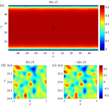
While the foregoing diagnostics (figure 3) have convincingly validated our closure models, it is still interesting to determine how well the sandpaper theory captures the physical mechanisms at play. For that, we first turn to one of the simulations in the fast-flow range. Figure 4 presents the flow pattern realized at  $t = 100$ in the experiment performed with
 ${U_{ini}} = 0.5$. The key feature of the fast-flow theory is the homogenization of the small-scale potential vorticity (3.2). This tendency is spectacularly manifested in patterns of
 $\varsigma$ (figure 4b) and
 $- \eta$ (figure 4c) plotted over a small area marked in figure 4(a) – patterns that are nearly identical in all fine detail.
The representative fully developed fast-flow state  $({U_{ini}} = 0.5,\ t = 100)$. Panel (a) shows the zonal velocity in the northern
 $(y > 0)$ part of the computational domain. Panel (b) presents the magnified view of vorticity in the square area marked in (a). The corresponding pattern of
 $- \eta $ is shown in (c).

To offer a more quantitative analysis of the homogenization tendency, we compute the correlation coefficient
 \begin{equation}{c_1} =- \frac{{{{\langle \varsigma \eta \rangle }_\varOmega }}}{{\sqrt {{{\langle {\varsigma ^2}\rangle }_\varOmega }{{\langle {\eta ^2}\rangle }_\varOmega }} }}.\end{equation}
For the state shown in figure 4,  ${c_1} = 0.9470$, which supports (3.2). In addition to the instantaneous correlation, we also introduce its temporal average
 \begin{equation}{C_1} = {\langle {c_1}\rangle _{0.5{t_0} < t < {t_0}}}.\end{equation}
The instantaneous correlation coefficients exhibit very limited variation in time in the fully developed flows, and generally  ${C_1} \approx {c_1}$. For the simulation in figure 4,
 ${C_1} = 0.9468$.
For the slow-flow regime, the leading-order balance according to the asymptotic theory (§ 3.2) is between  ${A_{ad}} = {u_{ls}}(\partial \eta /\partial x)$ and
 ${A_{diss}} = \nu {\nabla ^4}\psi $.
 ${A_{ad}}$ can be physically interpreted as the tendency of water columns to change their rotation rate due to stretching (squeezing) after being advected by the large-scale flow into the deeper (shallower) regions. Term
 ${A_{diss}}$, on the other hand, represents the frictional spin down. The anticipated balance of
 ${A_{ad}}$ and
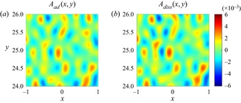
 ${A_{diss}}$ is readily confirmed by figure 5, which presents these quantities for one of the slow-flow simulations
 $({U_{ini}} = 5 \times {10^{ - 3}})$. In figure 5,
 ${A_{ad}}$ and
 ${A_{diss}}$ are plotted over a small area
 $- 1 < x < 1$,
 $24 < y < 26$, making it possible to visually compare their very similar patterns. For a more quantitative assessment, we introduce the instantaneous correlation coefficient
 $({c_2})$ and its temporal average
 $({C_2})$
 \begin{equation}{c_2} = \frac{{{{\langle {A_{ad}}{A_{diss}}\rangle }_\varOmega }}}{{\sqrt {{{\langle A_{ad}^2\rangle }_\varOmega }{{\langle A_{diss}^2\rangle }_\varOmega }} }},\quad {C_2} = {\langle {c_2}\rangle _{0.5{t_0} < t < {t_0}}}.\end{equation}
For the experiment in figure 5, we obtain  ${c_2} = 0.933$ at
 $t = 100$ and
 ${C_2} = 0.941$.
The representative fully developed slow-flow state  $({U_{ini}} = 5 \times {10^{ - 3}},\ t = 100)$. The advective
 $({A_{ad}})$ and diffusive
 $({A_{diss}})$ components of the expected leading-order balance are shown in (a) and (b), respectively.

In figure 6, we consolidate the estimates of time-mean correlation coefficients  $({C_1},{C_2})$ from all zonal-flow experiments and plot them as a function of
 ${u_{av}}$. The results illustrate the transition from the advective-dissipative balance realized at low speeds
 $({C_1} \ll 1, {C_2} \approx 1)$ to the homogenization of PV for swift currents
 $({C_1} \approx 1,\ {C_2} \ll 1)$.
The correlation coefficients  ${C_1}$ (red curve) and
 ${C_2}$ (blue curve) are plotted as functions of the average flow speed
 ${u_{av}}$. In relatively swift flows,
 ${C_1} \approx 1$, which is consistent with (3.2) and reflects the homogenization of PV. In weak flows,
 ${C_2} \approx 1$, which supports the advective-dissipative balance (3.11).

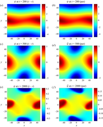
Figures 7 and 8 present an even more stringent test of the hybrid sandpaper model (§ 3.3). Here, we examine the non-zonal flow initiated by
 \begin{equation}{u_{ini}} = {U_{ini}}\,\textrm{tanh}(5\,\textrm{sin}(2{\rm \pi} yL_y^{ - 1})),\quad {v_{ini}} = 0.1{U_{ini}}\,\textrm{sin}(2{\rm \pi} xL_x^{ - 1}),\end{equation}
and compare the topography-resolving simulation with the corresponding parametric solution based on (3.26). In the following experiments, we use  ${U_{ini}} = 0.2$, which places the initial current in the category of fast flows. However, as the simulations are extended in time and velocities throughout the domain gradually reduce, these systems transition first into the intermediate-flow and, subsequently, the slow-flow regime. Thus, the analysis of the entire evolutionary pattern makes it possible to assess the performance of the hybrid sandpaper model in all three dynamically dissimilar regimes.
The snapshots of the streamfunction at t = 200, 500 and 2000 in the topography-resolving (a,c,e) and parametric (b,d, f) simulations.

The time series of mean kinetic energy. The topography-resolving, parametric and flat-bottom simulations are indicated by red, blue and black curves, respectively.

Since the parametric simulation does not require resolving rough topography and the associated small-scale flow features, it was performed on a relatively coarse grid with  $({N_x},{N_y}) = (256,256)$. Both simulations, topography resolving and parametric, were extended for 2000 time units. The results leave no doubt about the efficacy of the sandpaper theory. The flow fields in these simulations (figure 7) closely follow each other for most of the integration interval. Only in their final stages
 $(t > 1000)$ do these solutions visibly diverge. The temporal records of the kinetic energy (figure 8) further reinforce and quantify this conclusion. Until
 $t = 1000$, which is dimensionally equivalent to
 ${t^\ast } \approx 100\ \textrm{days}$, the relative differences in the kinetic energy does not exceed 5 %. We also emphasize the dramatic dissimilarity in the evolution of the corresponding flat-bottom simulation, also shown in figure 8. During these experiments, the kinetic energy in the topography-resolving and parametric simulations plunged by more than two orders of magnitude. In the flat-bottom run, it reduced by merely 12 %.
4.3. Other evolutionary patterns
A series of simulations exemplified by the experiments in § 4.2 indicate that the slow-hybrid-fast framework adequately describes the evolution of large-scale flows for the oceanographically relevant range of submesoscale eddy viscosities  $1\ {\textrm{m}^2}\ {\textrm{s}^{ - 1}}\lesssim{\nu ^\ast }\lesssim 100\ {\textrm{m}^2}\ {\textrm{s}^{ - 1}}$ (e.g. Li, Sun, & Xu Reference Li, Sun and Xu2018). The defining feature of these systems is relatively low values of the effective Taylor numbers
 $Ta \equiv f_0^{{\ast} 2}{L^{{\ast} 4}}/{\nu ^{{\ast} 2}}\lesssim O({10^6})$. However, some reflection suggests that expanding the analysis beyond this strongly dissipative regime is bound to reveal a fundamentally different dynamics.
In particular, we note that a large-scale current can transition into a PV-homogenized state satisfying (3.2) only if it is relatively swift to begin with:  $U\gtrsim\eta $. This implies that the fast-flow model (§ 4.1) cannot in principle represent the regime in which
 \begin{equation}{U^\ast } \ll \frac{{{\eta ^\ast }f_0^\ast {L^\ast }}}{{H_0^\ast }}.\end{equation}
Likewise, the advective-dissipative balance  ${u_{ls}}(\partial \eta /\partial x) \approx \nu {\nabla ^4}\psi $ – the cornerstone of the slow-flow theory – is unlikely to be realized in systems with weak friction
 \begin{equation}{\nu ^\ast } \ll \frac{{{\eta ^\ast }f_0^\ast {L^{{\ast} 2}}}}{{H_0^\ast }}.\end{equation}
Thus, the present version of the sandpaper theory (§ 3) does not capture systems with parameters concurrently satisfying both (4.15) and (4.16).
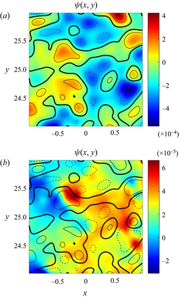
To bring some insight into the dynamics of such flows, we perform a series of simulations analogous to those in figure 4 in which Ro is systematically decreased and Re is increased. These experiments reveal two well-defined evolutionary patterns, the Taylor-column and the topographic Rossby wave regime, and various outcomes that are less clear cut. The Taylor-column regime tends to be realized for  ${10^{ - 4}} < {U_{ini}} < {10^{ - 3}}$ and
 $Ta\gtrsim {10^{20}}$. In this scenario, the initially uniform flow gradually reorganizes into recirculating patterns with fluid trapped in their interior. A representative experiment is shown in figure 9(a). Here we present a magnified view of the streamfunction over a small area
 $- 1 < x < 1$,
 $24 < y < 26$, superimposed on the contours of the topography. These diagnostics reveal the alignment of the flow along the isobaths in a spectacular manifestation of the topographic steering effect. The eddies in figure 9(a) are quasi-steady and centred directly above the underwater hills and valleys. However, when the initial velocity is further reduced to
 ${U_{ini}} < {10^{ - 4}}$, the Taylor-column regime gives way to the continuously oscillating pattern that we interpret as a disorganized field of topographic Rossby waves (figure 9b). In contrast to the Taylor-column regime, strong perturbations in figure 9(b) are mostly concentrated on the topographic slopes. Large-scale flows in the Taylor-column and topographic-wave regimes are characterized by comparable spin-down rates. While of limited relevance to the ocean, slow non-dissipative systems exemplified by the states in figure 9 are of interest in their own right and should be explored further for completeness.
Representative flow patterns in the Taylor-column (a) and topographic-wave (b) regimes. The initial velocity of  ${U_{ini}} = 2 \times {10^{ - 3}}$ was used in (a), whereas the simulation in (b) was performed with
 ${U_{ini}} = 2 \times {10^{ - 4}}$. In both cases,
 $\nu = {10^{ - 6}}$ and
 $t = 1000$. The isobaths with
 $\eta =- 0.07$, 0 and 0.07 are indicated by the dashed, heavy solid and light solid curves, respectively.

5. The multilayer model
The governing equations for the multilayer quasi-geostrophic rigid-lid model (e.g. Pedlosky 1987) are
 \begin{align}\left\{
{\begin{array}{*{20}{@{}ll@{}}} {\dfrac{{\partial q_1^\ast
}}{{\partial {t^\ast }}} + J(\psi_1^\ast ,q_1^\ast ) +
{\beta^\ast }\dfrac{{\partial \psi_1^\ast }}{{\partial
{x^\ast }}} = {\nu^\ast }{\nabla^4}\psi_1^\ast
,}&{q_1^\ast= {\nabla^2}\psi_1^\ast+ \dfrac{{f{{_0^\ast
}^2}}}{{{{g^{\prime}}^\ast }H_1^\ast }}(\psi_2^\ast-
\psi_1^\ast ),}\\ {\begin{array}{@{}l@{}}\dfrac{{\partial q_i^\ast }}{{\partial
{t^\ast }}} + J(\psi_i^\ast ,q_i^\ast ) + {\beta^\ast
}\dfrac{{\partial \psi_i^\ast }}{{\partial {x^\ast }}} =
{\nu^\ast }{\nabla^4}\psi_i^\ast ,\\ \quad i = 2, \ldots ,(n -
1)\end{array}}&{q_i^\ast= {\nabla^2}\psi_i^\ast+ \dfrac{{f{{_0^\ast
}^2}}}{{{{g^{\prime}}^\ast }H_i^\ast }}(\psi_{i - 1}^\ast+
\psi_{i + 1}^\ast- 2\psi_i^\ast ),}\\ {\begin{array}{@{}l@{}}\dfrac{{\partial
q_n^\ast }}{{\partial {t^\ast }}} + J(\psi_n^\ast ,q_n^\ast
) + {\beta^\ast }\dfrac{{\partial \psi_n^\ast }}{{\partial
{x^\ast }}} \\ \quad = {\nu^\ast }{\nabla^4}\psi_n^\ast-
{\gamma^\ast }{\nabla^2}\psi_n^\ast ,\end{array}}&{q_n^\ast=
{\nabla^2}\psi_n^\ast+ \dfrac{{f{{_0^\ast
}^2}}}{{{{g^{\prime}}^\ast }H_n^\ast }}(\psi_{n - 1}^\ast{\,-\,}
\psi_n^\ast ) {\,+\,} f_0^\ast \dfrac{{{\eta^\ast }}}{{H_n^\ast
}},} \end{array}}
\right.\end{align}
where  $\psi _i^\ast $ is the streamfunction in layer i and
 $H_i^\ast $ is the reference layer thickness. The reduced gravity is denoted by
 ${g^{\prime\ast} } = {g^\ast }(\varDelta {\rho ^\ast }/\rho _0^\ast )$, where
 ${g^\ast } \approx 9.8\ \textrm{m}\ {\textrm{s}^{ - 2}}$ is the standard gravity, and
 $\rho _0^\ast $ is the reference density. We assume identical density differences between adjacent layers
 $\varDelta {\rho ^\ast } = \rho _i^\ast- \rho _{i - 1}^\ast $, although the generalization to variable
 $\varDelta {\rho ^\ast }$ is straightforward.
The non-dimensionalization of (5.1) is based on (2.3), and the lowest layer depth  $H_n^\ast $ is used as a unit of topographic height
 \begin{equation}{\eta ^\ast } = H_n^\ast \eta. \end{equation}
In non-dimensional units, system (5.1) reduces to
 \begin{align}\left\{
{\begin{array}{*{20}{@{}ll@{}}} {\dfrac{{\partial
{q_1}}}{{\partial t}} + J({\psi_1},{q_1}) + \beta
\dfrac{{\partial {\psi_1}}}{{\partial x}} = \nu
{\nabla^4}{\psi_1},}&{{q_1} = {\nabla^2}{\psi_1} +
{F_1}({\psi_2} - {\psi_1}),}\\ {\begin{array}{@{}l@{}}\dfrac{{\partial
{q_i}}}{{\partial t}} + J({\psi_i},{q_i}) + \beta
\dfrac{{\partial {\psi_i}}}{{\partial x}} = \nu
{\nabla^4}{\psi_i},\\ \quad i = 2, \ldots ,(n - 1)\end{array}}&{{q_i} =
{\nabla^2}{\psi_i} + {F_i}({\psi_{i - 1}} + {\psi_{i + 1}}
- 2{\psi_i}),}\\ {\begin{array}{@{}l@{}} \dfrac{{\partial {q_n}}}{{\partial t}} +
J({\psi_n},{q_n}) + \beta \dfrac{{\partial
{\psi_n}}}{{\partial x}}\\ \quad= \nu {\nabla^4}{\psi_n} - \gamma
{\nabla^2}{\psi_n},\end{array}}&{{q_n} = {\nabla^2}{\psi_n} +
{F_n}({\psi_{n - 1}} - {\psi_n}) + \eta ,} \end{array}}
\right.\end{align}
where  ${F_i} = f_0^2{L^2}/g^{\prime}{H_i}$ is the inverse Burger number.
The fast-flow limit (3.1) was considered by Radko (Reference Radko2022b), resulting in
 \begin{align}\left\{
{\begin{array}{*{20}{@{}ll@{}}}
{\dfrac{{\partial {{\bar{q}}_1}}}{{\partial t}} + J({{\bar{\psi }}_1},{{\bar{q}}_1}) + \beta \dfrac{{\partial {{\bar{\psi
}}_1}}}{{\partial x}} = \nu {\nabla^4}{{\bar{\psi }}_1},}&{{{\bar{q}}_1} = {\nabla^2}{{\bar{\psi }}_1} +
{F_1}({{\bar{\psi }}_2} - {{\bar{\psi }}_1}),}\\
{\begin{array}{@{}l@{}}\dfrac{{\partial {{\bar{q}}_i}}}{{\partial t}} + J({{\bar{\psi }}_i},\quad {{\bar{q}}_i}) + \beta \dfrac{{\partial
{{\bar{\psi }}_i}}}{{\partial x}} = \nu {\nabla^4}{{\bar{\psi }}_i},\\
\quad i = 2, \ldots ,(n - 1),\end{array}}&{{{\bar{q}}_i} = {\nabla^2}{{\bar{\psi }}_i} +
{F_i}({{\bar{\psi }}_{i - 1}} + {{\bar{\psi }}_{i + 1}} -
2{{\bar{\psi }}_i}),}\\ {\begin{array}{@{}l@{}}\dfrac{{\partial
{{\bar{q}}_n}}}{{\partial t}} + J({{\bar{\psi
}}_n},{{\bar{q}}_n}) + \beta \dfrac{{\partial {{\bar{\psi
}}_n}}}{{\partial x}} + {D_{fast}}\\\quad = \nu
{\nabla^4}{{\bar{\psi }}_n} - \gamma {\nabla^2}{{\bar{\psi
}}_n},\end{array}}&{{{\bar{q}}_n} = {\nabla^2}{{\bar{\psi }}_n} +
{F_n}({{\bar{\psi }}_{n - 1}} - {{\bar{\psi }}_n}) +
{\eta_L}.} \end{array}}
\right.\end{align}
The topographic forcing term  $({D_{fast}})$ appears only in the bottom layer equation, and it takes the form of
 \begin{equation}{D_{fast}} = {G_{fast}}\left( {\frac{\partial }{{\partial x}}\left( {\frac{{{v_n}}}{{u_n^2 + v_n^2}}} \right) - \frac{\partial }{{\partial y}}\left( {\frac{{{u_n}}}{{u_n^2 + v_n^2}}} \right)} \right),\quad {G_{fast}} = 2{\rm \pi} \int {{{|{{{\tilde{\eta }}_S}} |}^2}\left( {\frac{\gamma }{\kappa } + \nu \kappa } \right)\textrm{d}\kappa } ,\end{equation}
where  $({u_n},{v_n}) = ( - \partial {\psi _n}/\partial y,\partial {\psi _n}/\partial x)$.
The theory development for slow-flow limit (3.6) parallels its barotropic counterpart (§ 3.2) and is presented in the abbreviated form. We adopt the scaling system in (3.6) and (3.9), and rescale  ${F_i}$ as
 \begin{equation}{F_i} = {\varepsilon ^2}F_i^{(0)}.\end{equation}
The solution in each layer i is then sought in terms of power series
 \begin{equation}{\psi _i} = \varepsilon \psi _i^{(1)}(X,Y,T) + {\varepsilon ^3}\psi _i^{(3)}(X,Y,x,y,T) + O({\varepsilon ^4}).\end{equation}
The leading-order  $O({\varepsilon ^4})$ balance in all layers except for the lowest one is trivially satisfied by
 \begin{equation}\psi _i^{(3)} = 0,\quad i = 1, \ldots ,(n - 1),\end{equation}
whereas for the bottom layer, it takes the form
 \begin{equation}\frac{{\partial \psi _n^{(1)}}}{{\partial X}}\frac{{\partial {\eta _{S0}}}}{{\partial y}} - \frac{{\partial \psi _n^{(1)}}}{{\partial Y}}\frac{{\partial {\eta _{S0}}}}{{\partial x}} = {\nu _0}{\nabla ^4}\psi _n^{(3)}.\end{equation}
The evolutionary large-scale equations are obtained by averaging the  $O({\varepsilon ^6})$ balances in
 $(x,y)$. The resulting expressions are then rewritten in terms of the original variables, leading to
 \begin{align}\left\{
{\begin{array}{*{20}{@{}ll@{}}} {\dfrac{{\partial
{{\bar{q}}_1}}}{{\partial t}} + J({{\bar{\psi
}}_1},{{\bar{q}}_1}) + \beta \dfrac{{\partial {{\bar{\psi
}}_1}}}{{\partial x}} = \nu {\nabla^4}{{\bar{\psi
}}_1},}&{{{\bar{q}}_1} = {\nabla^2}{{\bar{\psi }}_1} +
{F_1}({{\bar{\psi }}_2} - {{\bar{\psi }}_1}),}\\
{\begin{array}{@{}l@{}}\dfrac{{\partial {{\bar{q}}_i}}}{{\partial t}} +
J({{\bar{\psi }}_i},{{\bar{q}}_i}) + \beta \dfrac{{\partial
{{\bar{\psi }}_i}}}{{\partial x}} = \nu
{\nabla^4}{{\bar{\psi }}_i},\\ \quad i = 2, \ldots ,(n -
1)\end{array}}&{{{\bar{q}}_i} = {\nabla^2}{{\bar{\psi }}_i} +
{F_i}({{\bar{\psi }}_{i - 1}} + {{\bar{\psi }}_{i + 1}} -
2{{\bar{\psi }}_i}),}\\ {\begin{array}{@{}l@{}}\dfrac{{\partial
{{\bar{q}}_n}}}{{\partial t}} + J({{\bar{\psi
}}_n},{{\bar{q}}_n}) + \beta \dfrac{{\partial {{\bar{\psi
}}_n}}}{{\partial x}} + {D_{slow}}\\ \quad = \nu
{\nabla^4}{{\bar{\psi }}_n} - \gamma {\nabla^2}{{\bar{\psi
}}_n},\end{array}}&{{{\bar{q}}_n} = {\nabla^2}{{\bar{\psi }}_n} +
{F_n}({{\bar{\psi }}_{n - 1}} - {{\bar{\psi }}_n}) +
{\eta_L},} \end{array}}
\right.\end{align}
where  ${\bar{\psi }_i} = \varepsilon \psi _i^{(1)}$, and
 \begin{equation}{D_{slow}} = {G_{slow}}\left( {\frac{{\partial {{\bar{v}}_n}}}{{\partial x}} - \frac{{\partial {{\bar{u}}_n}}}{{\partial y}}} \right),\quad {G_{slow}} = {\rm \pi}\int {\frac{{{{|{{{\tilde{\eta }}_S}} |}^{\,2}}}}{{\nu \kappa }}\,\textrm{d}\kappa } .\end{equation}
Systems (5.4) and (5.10) represent the limits of slow and fast flows. A challenge that naturally arises at this point is the development of a universal framework that would apply to a wide range of velocities. We also insist that such a framework must be fully consistent with (5.4) and (5.10) in the limits of high and low velocities, respectively. Fortunately, the structural similarity of the topographic forcing terms (5.5) and (5.11) to their homogeneous counterparts (§ 3) makes it possible to adopt the previously developed and tested hybrid model (3.25) with only minimal modifications
 \begin{align}{D_{hybrid}} &=
\frac{\partial }{{\partial x}}\left[{\bar{v}_n}\,\bar{V}_n^{ -
1}{F_C}\,\textrm{exp}\left\{ - \sqrt {1 + {{\ln
}^2}({{\bar{V}}_n}V_C^{ - 1})} \right\} \right]\notag\\ &\quad - \frac{\partial
}{{\partial y}}\left[{\bar{u}_n}\,\bar{V}_n^{ -
1}{F_C}\,\textrm{exp}\left\{ - \sqrt {1 + {{\ln
}^2}({{\bar{V}}_n}V_C^{ - 1})} \right\} \right],\end{align}
where  ${\bar{V}_n} = \sqrt {\bar{u}_n^2 + \bar{v}_n^2} $. Replacing
 ${D_{fast}}$ and
 ${D_{slow}}$ in (5.4) and (5.10) by the hybrid expression (5.12) completes the development of a general theory of flow forcing by rough topography – the main objective of our study.
To simplify the implementation of the proposed theory in future investigations, we also include the dimensional expression of the topographic forcing
 \begin{align}D_{hybrid}^\ast &=
\frac{\partial }{{\partial {x^\ast }}}\left[
{\frac{{\bar{v}_n^\ast }}{{\bar{V}_n^\ast }}F_C^\ast
\,\textrm{exp}\left\{ { - \sqrt {1 + {{\ln }^2}\left(
{\frac{{\bar{V}_n^\ast }}{{V_C^\ast }}} \right)} }
\right\}} \right]\notag\\ &\quad - \frac{\partial }{{\partial {y^\ast
}}}\left[ {\frac{{\bar{u}_n^\ast }}{{\bar{V}_n^\ast
}}F_C^\ast \,\textrm{exp}\left\{ { - \sqrt {1 + {{\ln
}^2}\left( {\frac{{\bar{V}_n^\ast }}{{V_C^\ast }}} \right)}
} \right\}}
\right],\end{align}
where  $\bar{V}_n^\ast= \sqrt {\bar{u}_n^{{\ast} 2} + \bar{v}_n^{{\ast} 2}} $,
 $V_C^\ast= \sqrt {G_{fast}^\ast{/}G_{slow}^\ast }$,
 $F_C^\ast= \sqrt {G_{fast}^\ast G_{slow}^\ast }$ and
 \begin{equation}G_{fast}^\ast= \frac{{2{\rm \pi} f_0^{{\ast} 2}}}{{H_n^{{\ast} 2}}}\int {{{|{\tilde{\eta }_S^\ast } |}^2}\left( {\frac{{{\gamma^\ast }}}{{{\kappa^\ast }}}\, + {\nu^\ast }{\kappa^\ast }} \right)\textrm{d}{\kappa ^\ast }} ,\quad G_{slow}^\ast= \frac{{{\rm \pi} f_0^{{\ast} 2}}}{{H_n^{{\ast} 2}}}\int {\frac{{{{|{\tilde{\eta }_S^\ast } |}^2}}}{{{\nu ^\ast }{\kappa ^\ast }}}\,\textrm{d}{\kappa ^\ast }} .\end{equation}
Term (5.13) can be introduced in the bottom layer equation in (5.1) to represent the effects of unresolved bathymetry. We also note that adding  $D_{hybrid}^\ast $ to the potential vorticity equation is equivalent to modifying the horizontal momentum equations as follows:
 \begin{equation}\left\{ \begin{array}{@{}l@{}}
\dfrac{{\partial u_n^\ast }}{{\partial {t^\ast }}} +
u_n^\ast \dfrac{{\partial u_n^\ast }}{{\partial {x^\ast }}}
+ v_n^\ast \dfrac{{\partial u_n^\ast }}{{\partial {y^\ast
}}} - {f^\ast }v_n^\ast=- \dfrac{1}{{\rho_n^\ast
}}\dfrac{{\partial p_n^\ast }}{{\partial {x^\ast }}} -
M_x^\ast+ {\nu^\ast }{\nabla^2}u_n^\ast ,\\
\dfrac{{\partial v_n^\ast }}{{\partial {t^\ast }}} +
u_n^\ast \dfrac{{\partial v_n^\ast }}{{\partial {x^\ast }}}
+ v_n^\ast \dfrac{{\partial v_n^\ast }}{{\partial {y^\ast
}}} + {f^\ast }u_n^\ast=- \dfrac{1}{{\rho_n^\ast
}}\dfrac{{\partial p_n^\ast }}{{\partial {y^\ast }}} -
M_y^\ast+ {\nu^\ast }{\nabla^2}v_n^\ast , \end{array}
\right.\end{equation}
where  $p_n^\ast $ is the pressure field in the bottom layer, and
 \begin{equation}\left\{ \begin{array}{@{}l} M_x^\ast= \dfrac{{\bar{u}_n^\ast }}{{\bar{V}_n^\ast }}F_C^\ast \,\textrm{exp}\left\{ { - \sqrt {1 + {{\ln }^2}\left( {\dfrac{{\bar{V}_n^\ast }}{{V_C^\ast }}} \right)} } \right\},\\ M_y^\ast= \dfrac{{\bar{v}_n^\ast }}{{\bar{V}_n^\ast }}F_C^\ast \,\textrm{exp}\left\{ { - \sqrt {1 + {{\ln }^2}\left( {\dfrac{{\bar{V}_n^\ast }}{{V_C^\ast }}} \right)} } \right\}. \end{array} \right.\end{equation}
Formulation (5.16) makes it possible to implement the hybrid parameterization of rough topography in multilayer general circulation models (e.g. Bleck Reference Bleck2002).
6. Discussion
At the time of this writing, it is generally accepted that rough topography can strongly influence the intensity and variability of large-scale and mesoscale flows in the ocean (e.g. LaCasce et al. Reference LaCasce, Escartin, Chassignet and Xu2019; Radko Reference Radko2020; Gulliver & Radko Reference Gulliver and Radko2022). However, our understanding of the specific mechanisms of bathymetric control and our ability to concisely represent it in theoretical and coarse-resolution numerical models remain limited. Our recent efforts (Radko Reference Radko2022a,Reference Radkob) have led to the development of the analytical ‘sandpaper’ model that captures the effects of irregular topographic features, provided that the spectrum of sea-floor depth is known. The model of Radko (Reference Radko2022a,Reference Radkob) performed well for relatively fast flows but exhibited unphysical behaviour in the low-speed limit. This complication motivates the present attempt to formulate the second-generation sandpaper model that is uniformly valid for all oceanographically relevant velocity values.
To this end, we have explored two fundamentally different regimes, represented by the asymptotic limits of low and high flow speeds. Both limits were treated using conventional multiscale methods (e.g. Mei & Vernescu Reference Mei and Vernescu2010), leading to the analytical description of large-scale forcing by rough bathymetry. We also took advantage of the dynamical transparency of multiscale theories, which made it possible to unambiguously identify the essential physical mechanisms at play. In the fast-flow regime, the key phenomenon is the homogenization of potential vorticity. Homogenization controls the dynamics of small-scale topographically generated eddies and the associated Reynolds stresses. Surprisingly, the eddy stresses dominate the net topographic forcing of swift large-scale flows, whereas the form drag, which is invoked in flow-topography interaction theories more often, turned out to be largely inconsequential. However, the situation changes cardinally for slow currents. In this regime, the small-scale dynamics is governed by the balance between the torque associated with the stretching/squeezing of water columns and their frictional spin down. The topographic form drag becomes the primary large-scale forcing mechanism, while the Reynolds stresses are weak and dynamically insignificant. These mechanisms control the flow-topography interaction in both homogeneous (§ 3) and layered (§ 5) models.
From a pragmatic perspective, the key advancement brought by this study is a generic hybrid model that encompasses both slow-flow and fast-flow limits. In essence, this model represents a rigorous asymptotics-based parameterization of the effects of rough topography. It naturally lends itself to the implementation in layered oceanic general circulation models, which are commonly used in climate prediction studies and for operational forecasting. Despite continuous progress in high-performance computing, roughness-resolving models will not be used for extended global simulations in the foreseeable future. The sandpaper model, on the other hand, is expected to improve the accuracy of simulations without the major increase in resolution and associated computational costs.
The explicit nature of the sandpaper model also opens a pathway for in-depth theoretical analyses of the myriad processes that are affected by the bottom roughness. Future studies should address the impact of irregular topography on subtropical and subpolar gyres, the Antarctic Circumpolar Current, large-scale waves, baroclinic and barotropic instabilities and boundary currents – among many other oceanic systems. The existing evidence indicates that the impact of bottom roughness is profound, and the sandpaper theory can make such problems ultimately tractable.
On a more technical side, it would be highly desirable to transition from the quasi-geostrophic framework to more general systems, including the shallow-water and, eventually, full Navier–Stokes equations. The quasi-geostrophic approximation is assumed here to minimize complexity and enhance dynamic transparency. However, the flow speed at some locations in the ocean can exceed its formal applicability limits. Therefore, new versions of the sandpaper theory should be capable of representing strongly nonlinear systems with order-one Rossby numbers. Recent progress in this direction has been encouraging. Gulliver & Radko (Reference Gulliver and Radko2023) abandoned the quasi-geostrophic approximation and performed a series of simulations of flows over rough topography with the barotropic Navier–Stokes model. The key features of these experiments – including the PV-homogenization and the inverse velocity-drag relation – proved to be consistent with the sandpaper theory.
Acknowledgements
The author thanks N. Balmforth and the anonymous reviewers for helpful comments.
Funding
Support of the National Science Foundation (grant OCE 1828843) is gratefully acknowledged.
Declaration of interests
The author reports no conflict of interest.
Appendix A. Auxiliary steps in the development of the asymptotic slow-flow model
The objective of the following analysis is the explicit expression of the topographic forcing function (3.13) in terms of the properties of the large-scale flow. The calculations are conveniently performed in the flow-following small-scale coordinate system:
 \begin{equation}\left\{ \begin{array}{@{}l} x^{\prime} = x\,\textrm{cos}\,\theta + y\,\textrm{sin}\,\theta ,\\ y^{\prime} =- x\,\textrm{sin}\,\theta + y\,\textrm{cos}\,\theta \,. \end{array} \right.\end{equation}
The flow-orientation variable  $\theta$ in (A1) is defined by
 \begin{equation}\textrm{cos}(\theta ) =- \frac{1}{V}\frac{{\partial {\psi ^{(1)}}}}{{\partial Y}},\quad \textrm{sin}(\theta ) = \frac{1}{V}\frac{{\partial {\psi ^{(1)}}}}{{\partial X}},\end{equation}
where  $V = \sqrt {{{(\partial {\psi ^{(1)}}/\partial Y)}^2} + {{(\partial {\psi ^{(1)}}/\partial Y)}^2}}$. In the new coordinate system, (3.11) takes the form
 \begin{equation}V\frac{{\partial {\eta _{S0}}}}{{\partial x^{\prime}}} = {\nu _0}{\nabla ^4}{\psi ^{(3)}}\end{equation}
and (3.13) is written as
 \begin{equation}{D_{slow\ 0}} = \frac{\partial }{{\partial X}}({D_V}\,\textrm{sin}\,\theta + {D_U}\,\textrm{cos}\,\theta ) - \frac{\partial }{{\partial Y}}({D_V}\,\textrm{cos}\,\theta - {D_U}\,\textrm{sin}\,\theta ),\end{equation}
where
 \begin{equation}{D_V} = {\left\langle {{\psi^{(3)}}\frac{{\partial {\eta_{S0}}}}{{\partial x^{\prime}}}} \right\rangle _{x^{\prime},y^{\prime}}},\quad {D_U} = {\left\langle {{\psi^{(3)}}\frac{{\partial {\eta_{S0}}}}{{\partial y^{\prime}}}} \right\rangle _{x^{\prime},y^{\prime}}}.\end{equation}
The  ${D_U}$ term can be shown to be inconsequential based on its symmetries. Reversing the x’-orientation of small-scale bathymetry
 ${\eta _S} \to {\eta _S}( - x^{\prime},y^{\prime})$ reverses the sign of
 ${\psi ^{(3)}} \to - {\psi ^{(3)}}( - x^{\prime},y^{\prime})$, which, in turn, reverses the sign of
 ${D_U}$. Thus, any statistical averaging that assigns equal weights to a given pattern of
 ${\eta _S}$ and its mirror image results in the net cancellation of their contributions to
 ${D_U}$.
To obtain an explicit expression for  ${D_V}$, we eliminate
 $\partial {\eta _{S0}}/\partial x^{\prime}$ in (A5) using (A3), which yields
 \begin{equation}{D_V} = {V^{ - 1}}{\langle {\psi ^{(3)}}{\nu _0}{\nabla ^4}{\psi ^{(3)}}\rangle _{x^{\prime},y^{\prime}}}.\end{equation}
This expression is further simplified using the Parseval identity
 \begin{equation}{D_V} = {V^{ - 1}}\iint {{{\tilde{\psi }}^{(3)}} \cdot \textrm{conj}({\nu _0}{\kappa ^4}{{\tilde{\psi }}^{(3)}})\,\textrm{d}k^{\prime}\,\textrm{d}l^{\prime}} ,\end{equation}
where  $(k^{\prime},l^{\prime})$ are the small-scale wavenumbers in the flow-following coordinate system and
 ${\kappa ^2} = {k^{\prime 2}} + {l^{\prime 2}}$. To evaluate the double integral in (A7), we use polar coordinates defined as
 \begin{equation}k^{\prime} = \kappa \,\textrm{cos}\,\varphi ,\quad l^{\prime} = \kappa \,\textrm{sin}\,\varphi ,\end{equation}
which further reduces (A7) to
 \begin{equation}{D_V} = {V^{ - 1}}\iint {{|{{{\tilde{\psi }}^{(3)}}(\kappa ,\varphi )} |^2}{\nu _0}{\kappa ^4}\kappa \,\textrm{d}\kappa \,\textrm{d}\varphi } .\end{equation}
Next,  ${D_V}$ is expressed in terms of the spectrum of small-scale topography. This is accomplished by applying the Fourier transform to (A3) and evaluating the squared absolute values of both sides of the resulting equation
 \begin{equation}{V^2}{\kappa ^2}\,\textrm{co}{\textrm{s}^2}\,\varphi {|{{{\tilde{\eta }}_{S0}}} |^2} = {({\nu _0}{\kappa ^4})^2}{|{{{\tilde{\psi }}^{(3)}}} |^2}.\end{equation}
In this study, we consider statistically isotropic spectra of topography, with  $\,{|{{{\tilde{\eta }}_{S0}}} |^2}$ fully determined by
 $\kappa $. For such patterns, we can conveniently link topography and streamfunction by integrating (A10) in
 $\varphi $
 \begin{equation}{\rm \pi} {V^2}{\kappa ^2}{|{{{\tilde{\eta }}_{S0}}} |^2} = {({\nu _0}{\kappa ^4})^2}\int {{{|{{{\tilde{\psi }}^{(3)}}} |}^2}\,\textrm{d}\varphi } ,\end{equation}
which reduces (A9) to
 \begin{equation}{D_V} = {\rm \pi}V\int {\frac{{\kappa {{|{{{\tilde{\eta }}_{S0}}} |}^{\,2}}}}{{{\nu _0}{\kappa ^2}}}\,\textrm{d}\kappa } .\end{equation}
Finally, we compute (A4):
 \begin{equation}{D_{slow\ 0}} = {G_{slow\ 0}}\left( {\frac{{{\partial^2}{\psi^{(1)}}}}{{\partial {X^2}}} + \frac{{{\partial^2}{\psi^{(1)}}}}{{\partial {Y^2}}}} \right),\end{equation}
where
 \begin{equation}{G_{slow\ 0}} = {\rm \pi}\int {\frac{{{{|{{{\tilde{\eta }}_{S0}}} |}^{\,2}}}}{{{\nu _0}\kappa }}\,\textrm{d}\kappa } .\end{equation}