2 Numerical method

2.1 Problem definition

Two connected axisymmetric, uncharged, conducting droplets of an incompressible, Newtonian fluid, with radius  $a$ , and viscosity $\unicode[STIX]{x1D707}_{i}$ is suspended in a dielectric, incompressible, Newtonian medium of viscosity  $\unicode[STIX]{x1D707}_{e}$ . Interfacial tension, $\unicode[STIX]{x1D6FE}$ is assumed to be constant between the droplet and the medium fluids. Other parameters used to characterize the fluids are the conductivities, $\unicode[STIX]{x1D70E}_{i}$ , $\unicode[STIX]{x1D70E}_{e}$ ( $R=\unicode[STIX]{x1D70E}_{e}/\unicode[STIX]{x1D70E}_{i}$ ) and dielectric constants, $\unicode[STIX]{x1D716}_{i}$ , $\unicode[STIX]{x1D716}_{e}$ ( $Q=\unicode[STIX]{x1D716}_{i}/\unicode[STIX]{x1D716}_{e}$ ). Here $i$ and $e$ are subscripts representing inner and outer fluids respectively. A uniform electric field ( $\boldsymbol{E}_{\mathbf{0}}$ , reference electric field) is considered to be applied across the drop. Analysis is done in the Stokes flow regime and thereby the Reynolds number is considered to be negligible and inertial terms in the Navier–Stokes equation are ignored. Ignoring gravity, the fluid motion is governed by the following equations:

(2.1) $$\begin{eqnarray}\displaystyle & \unicode[STIX]{x1D735}\boldsymbol{\cdot }\boldsymbol{u}_{\boldsymbol{i},\boldsymbol{e}}=0, & \displaystyle\end{eqnarray}$$

(2.2) $$\begin{eqnarray}\displaystyle & -\unicode[STIX]{x1D735}p_{i,e}+\unicode[STIX]{x1D706}\unicode[STIX]{x1D6FB}^{2}\boldsymbol{u}_{\boldsymbol{i},\boldsymbol{e}}=0, & \displaystyle\end{eqnarray}$$

where the viscosity ratio is defined as $\unicode[STIX]{x1D706}=\unicode[STIX]{x1D707}_{i}/\unicode[STIX]{x1D707}_{e}$ and $\unicode[STIX]{x1D707}_{e}=1$ and $\unicode[STIX]{x1D707}_{i}=\unicode[STIX]{x1D706}$ . Taylor’s leaky dielectric theory can be used to model the system and the equations are

(2.3a,b ) $$\begin{eqnarray}\boldsymbol{E}_{\boldsymbol{i},\boldsymbol{e}}=-\unicode[STIX]{x1D735}\unicode[STIX]{x1D719}_{i,e}\quad \text{and}\quad \unicode[STIX]{x1D6FB}^{2}\unicode[STIX]{x1D719}=0.\end{eqnarray}$$

The boundary conditions are given as,

(2.4a,b ) $$\begin{eqnarray}\unicode[STIX]{x1D748}_{i}n\boldsymbol{\cdot }\boldsymbol{E}_{\boldsymbol{i}}=\unicode[STIX]{x1D748}_{\boldsymbol{e}}\boldsymbol{n}\boldsymbol{\cdot }\boldsymbol{E}_{\boldsymbol{e}}\quad \text{and}\quad \boldsymbol{t}\boldsymbol{\cdot }\boldsymbol{E}_{\boldsymbol{i}}=\boldsymbol{t}\boldsymbol{\cdot }\boldsymbol{E}_{\boldsymbol{e}},\end{eqnarray}$$

where $\boldsymbol{n}$ and $\boldsymbol{t}$ are the outward unit normal and the unit tangent vectors at the interface respectively. The calculations here are presented for $\unicode[STIX]{x1D70E}_{i}/\unicode[STIX]{x1D70E}_{e}=1000$ thereby mimicking a water-in-oil system.

2.2 Boundary element formulation

The integral equations governing the normal electric field and the velocity field in Stokes flow (fluid flow) can be realized by reducing volume integrals of the governing equations to surface integrals using the divergence theorem. In the equations that follow, $C$ is the drop interface, $\boldsymbol{x}_{\boldsymbol{c}}$ is the evaluation point on the surface of the drop and $\boldsymbol{x}$ is the variable of integration. The terms of the equations are non-dimensionalized using $a$ (length scale), $\unicode[STIX]{x1D716}_{e}\unicode[STIX]{x1D716}_{o}E_{0}^{2}$ (stress) and $\unicode[STIX]{x1D707}_{e}/(\unicode[STIX]{x1D716}_{e}\unicode[STIX]{x1D716}_{o}E_{0}^{2})$ (time scale). In a cylindrical coordinate system the potential is $\unicode[STIX]{x1D719}=-E_{o}z$ , where $z$ is the coordinate along the axis of symmetry. At the interface of the two fluids, a Maxwell stress is induced on application of an electric field. Using the boundary conditions, this electric field at the interface is calculated (Baygents, Rivette & Stone Reference Baygents, Rivette and Stone1998) as,

(2.5) $$\begin{eqnarray}E_{ne}(\boldsymbol{x}_{\boldsymbol{c}})=\frac{2R}{1+R}\boldsymbol{n}(\boldsymbol{x}_{\boldsymbol{c}})\boldsymbol{\cdot }\boldsymbol{E}_{\mathbf{0}}(\boldsymbol{x}_{\boldsymbol{c}})-\left(\frac{1-R}{1+R}\right)\frac{\boldsymbol{n}(\boldsymbol{x}_{\boldsymbol{c}})}{2\unicode[STIX]{x03C0}}\boldsymbol{\cdot }\int _{C}\frac{(\boldsymbol{x}-\boldsymbol{x}_{\boldsymbol{c}})}{|\boldsymbol{x}-\boldsymbol{x}_{\boldsymbol{c}}|^{3}}E_{ne}(\boldsymbol{x})\,\text{d}C(\boldsymbol{x}),\end{eqnarray}$$

where $E_{ne}=\boldsymbol{n}\boldsymbol{\cdot }\boldsymbol{E}_{\boldsymbol{e}}$ and $R=\unicode[STIX]{x1D70E}_{e}/\unicode[STIX]{x1D70E}_{i}$ . To model a perfect conductor in a perfectly dielectric fluid, the value of $R$ is taken as 0.001. Using the boundary element method, the velocity at the surface of the drop is written in the integral form as (Pozrikidis Reference Pozrikidis1992)

(2.6) $$\begin{eqnarray}\displaystyle \boldsymbol{u}(\boldsymbol{x}_{\boldsymbol{c}}) & = & \displaystyle -\frac{1}{4\unicode[STIX]{x03C0}(1+\unicode[STIX]{x1D706})}\int _{C}\unicode[STIX]{x0394}\boldsymbol{f}(\boldsymbol{x})\boldsymbol{\cdot }\boldsymbol{G}(\boldsymbol{x},\boldsymbol{x}_{\boldsymbol{c}})\,\text{d}S(x)\nonumber\\ \displaystyle & & \displaystyle +\,\frac{1-\unicode[STIX]{x1D706}}{4\unicode[STIX]{x03C0}(1+\unicode[STIX]{x1D706})}\int _{C}\boldsymbol{n}(\boldsymbol{x})\boldsymbol{\cdot }\boldsymbol{T}(\boldsymbol{x},\boldsymbol{x}_{\boldsymbol{c}})\boldsymbol{\cdot }\boldsymbol{u}(\boldsymbol{x})\,\text{d}C(\boldsymbol{x}),\end{eqnarray}$$

where $\boldsymbol{G}$ and $\boldsymbol{T}$ are known kernel functions of the velocity and stress fields, respectively (Pozrikidis Reference Pozrikidis1992) and are given by $\boldsymbol{G}(\boldsymbol{x},\boldsymbol{x}_{\boldsymbol{c}})=(\boldsymbol{I}/|\boldsymbol{x}-\boldsymbol{x}_{\boldsymbol{c}}|)+((\boldsymbol{x}-\boldsymbol{x}_{\boldsymbol{c}})(\boldsymbol{x}-\boldsymbol{x}_{\boldsymbol{c}})/|\boldsymbol{x}-\boldsymbol{x}_{\boldsymbol{c}}|^{3})$ and $\boldsymbol{T}(\boldsymbol{x},\boldsymbol{x}_{\boldsymbol{c}})=-6((\boldsymbol{x}-\boldsymbol{x}_{\boldsymbol{c}})(\boldsymbol{x}-\boldsymbol{x}_{\boldsymbol{c}})(\boldsymbol{x}-\boldsymbol{x}_{\boldsymbol{c}})/|\boldsymbol{x}-\boldsymbol{x}_{\boldsymbol{c}}|^{5})$ . The force at the interface is given by $\unicode[STIX]{x0394}\boldsymbol{f}(\boldsymbol{x})=[\boldsymbol{n}(\boldsymbol{x})(\unicode[STIX]{x1D735}_{s}\boldsymbol{\cdot }\boldsymbol{n}(\boldsymbol{x})/Ca)-\unicode[STIX]{x1D70F}^{E}\boldsymbol{\cdot }\boldsymbol{n}(\boldsymbol{x})]$ , where $\unicode[STIX]{x1D735}_{s}\boldsymbol{\cdot }\boldsymbol{n}(\boldsymbol{x})$ is the mean curvature, $Ca=\unicode[STIX]{x1D716}_{e}\unicode[STIX]{x1D716}_{0}E_{0}^{2}/\unicode[STIX]{x1D6FE}$ (electrocapillary number) and the electric traction $\unicode[STIX]{x1D70F}^{\boldsymbol{E}}\boldsymbol{\cdot }\boldsymbol{n}(\boldsymbol{x})=\frac{1}{2}[((1-QR^{2})E_{ne}^{2}-(1-Q)E_{te}^{2})\boldsymbol{n}+2(1-QR)E_{ne}E_{te}\boldsymbol{t}]$ . For an infinitely conducting drop suspended in a dielectric medium, $R\ll 1$ , $E_{t}\rightarrow 0$ and the Maxwell stress is given by $\unicode[STIX]{x1D70F}^{\boldsymbol{E}}\boldsymbol{\cdot }\boldsymbol{n}(\boldsymbol{x})=\frac{1}{2}E_{ne}^{2}\boldsymbol{n}$ .

The drop shape is discretized into $N$ elements (typically 150 elements were used) using $N+1$ node points in cylindrical coordinates. Parametrized cubic splines are used to fit the node points and $E_{n}$ and $\boldsymbol{u}$ can be assumed to vary linearly between them. Once normal electric field is calculated, interfacial velocity is computed and the interface (nodes) is advanced using the explicit Euler method,

(2.7) $$\begin{eqnarray}\boldsymbol{x}_{\boldsymbol{s}}^{\boldsymbol{t}+\mathbf{1}}=\boldsymbol{x}_{\boldsymbol{ s}}^{\boldsymbol{t}}+\boldsymbol{u}(\boldsymbol{x}_{\boldsymbol{ s}})\unicode[STIX]{x0394}t.\end{eqnarray}$$

Convergence of the results, the choice of the time step size and the number of node points are discussed in the supplementary information available at https://doi.org/10.1017/jfm.2019.665.

3 Experimental

3.1 Experimental set-up and procedure

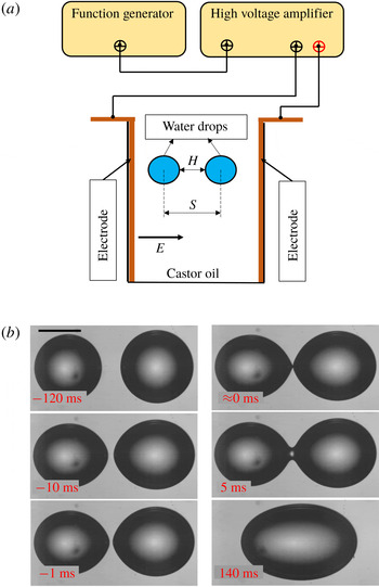
Castor oil of viscosity 650 cSt ( $25\,^{\circ }\text{C}$ ) purchased from Sigma-Aldrich was used without further purification. Deionized (DI) water of conductivity $\unicode[STIX]{x1D70E}=1.4\times 10^{-4}~\text{S}~\text{m}^{-1}$ was obtained from EVOQUA (Ultra Clear GP TWF UV UF TM). Figure 1(a) shows the schematic diagram of the experimental set-up. The experimental set-up consists of a rectangular cuvette ( $10~\text{mm}\times 10~\text{mm}$ ) where two parallel copper plate electrodes ( $45~\text{mm}\times 10~\text{mm}\times 1.5~\text{mm}$ ) are fixed onto the opposite walls of the cuvette. The copper electrodes are connected with a high voltage amplifier (Trek,  $5/80$ ). The amplitude of the voltage and the frequency of the AC signal are adjusted with the help of a function generator (Agilent, 33220A). The cuvette is filled with castor oil, and two DI water droplets are inserted with the help of a syringe. To capture the interaction and breakup of droplets we conducted high-speed videography ( $10\,000~\text{frames}~\text{s}^{-1}$ ) using a camera (Vision Research, Phantom v12). The camera is attached to a stereo zoom microscope (Nikon, C-FI230) to magnify the image. A fibre optics light source (Nikon, model: C-FI230) is used to provide sufficient light. The high-speed images are analysed using ImageJ. The experiments were conducted at room temperature ( $25\,^{\circ }\text{C}$ ).

Figure 1.

(a) Schematic diagram of experimental set-up. (b) Sequence of images showing approach, film drainage, rupture of film and coalescence of two DI water droplets in castor oil under an electric field ( $Ca=0.063$ ). Scale bar shown is $500~\unicode[STIX]{x03BC}\text{m}$ .

4 Results and discussion

Two DI water droplets in castor oil, parallel to the direction of applied electric field, are allowed to approach each other, come in contact and then either coalesce or non-coalesce. The critical electrocapillary number $Ca_{c}$ above which DI water droplets suspended in castor oil exhibit non-coalescence is 0.08 (Anand et al. Reference Anand, Roy, Naik, Juvekar and Thaokar2019). Figure 1(b) shows how at $Ca=0.063$ the two droplets approach each other, form a bridge and finally coalesce.

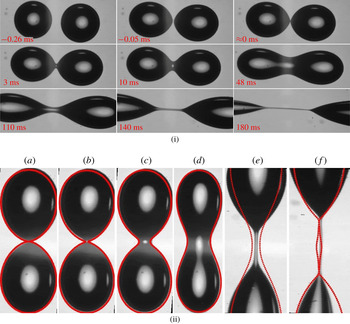
However, an interesting behaviour is observed when $Ca$ is beyond the critical value of 0.08. As shown in figure 2(i) the slightly asymmetric droplets approach each other and at contact, exhibit cone-dimple formation (Anand et al. Reference Anand, Roy, Naik, Juvekar and Thaokar2019). The resultant bridge then starts to grow in diameter, indicating tendency to coalesce. The figure 2(i) also shows that the diameter of the bridge continues to grow for a while whereafter the bridge starts to thin indicating higher capillary pressure at the centre, which pushes the liquid out and away from the bridge and finally the liquid bridge breaks down into tiny droplets.

Figure 2.

(i) Sequence of images showing approach, film drainage, rupture of film, initial bridge formation and thickening and then thinning of the bridge and further breakup of two DI water droplets in castor oil under an electric field ( $Ca=0.135$ ). Scale bar shown is $500~\unicode[STIX]{x03BC}\text{m}$ . (ii) Superimposed generated shape (with $\unicode[STIX]{x1D716}=1.928$ ) and further simulated results on experimental bridged droplets for DI water in castor oil- 650 cSt subjected to $3~\text{kV}~\text{cm}^{-1}$ ( $Ca=0.135\pm 0.007$ ) for various times (a)  $t=0$  ms, (b)  $t=3$  ms, (c)  $t=10$  ms, (d)  $t=48$  ms, (e)  $t=140$  ms, (f)  $t=180$  ms.

To investigate the dynamics of breakup after the formation of the bridge, it is essential to replicate the initial shape of the droplets in contact ( $t=0$  ms in figure 1 b), and allow them to evolve under electric field. Such a bridged drop is generated using the second Legendre polynomial $P_{2}(\cos \unicode[STIX]{x1D703})$ . Thus the initial drop profile is given by,

(4.1) $$\begin{eqnarray}r_{s}(\unicode[STIX]{x1D703})=1+\unicode[STIX]{x1D716}P_{2}(\cos \unicode[STIX]{x1D703}),\end{eqnarray}$$

where $r_{s}(\unicode[STIX]{x1D703})$ is the equation of the combined drop and $\unicode[STIX]{x1D716}$ can be varied to obtain the bridge width in reasonable agreement with experiments, as shown in figure 2(ii). Typically $\unicode[STIX]{x1D716}=1.9$ results in shapes that mimic figure 1(b) $t=5$  ms and figure 2(i) $t=0$  ms. Using this initial shape, numerical simulations employing the boundary element method (BEM) can be carried out to see the evolution of the drop. The agreement in shape between experiments and BEM is reasonable.

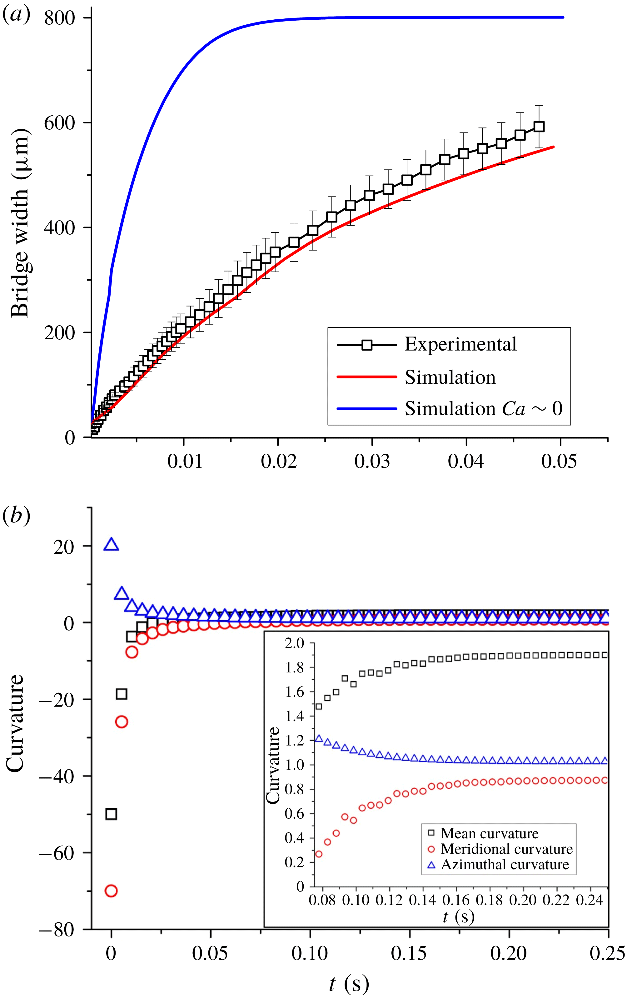
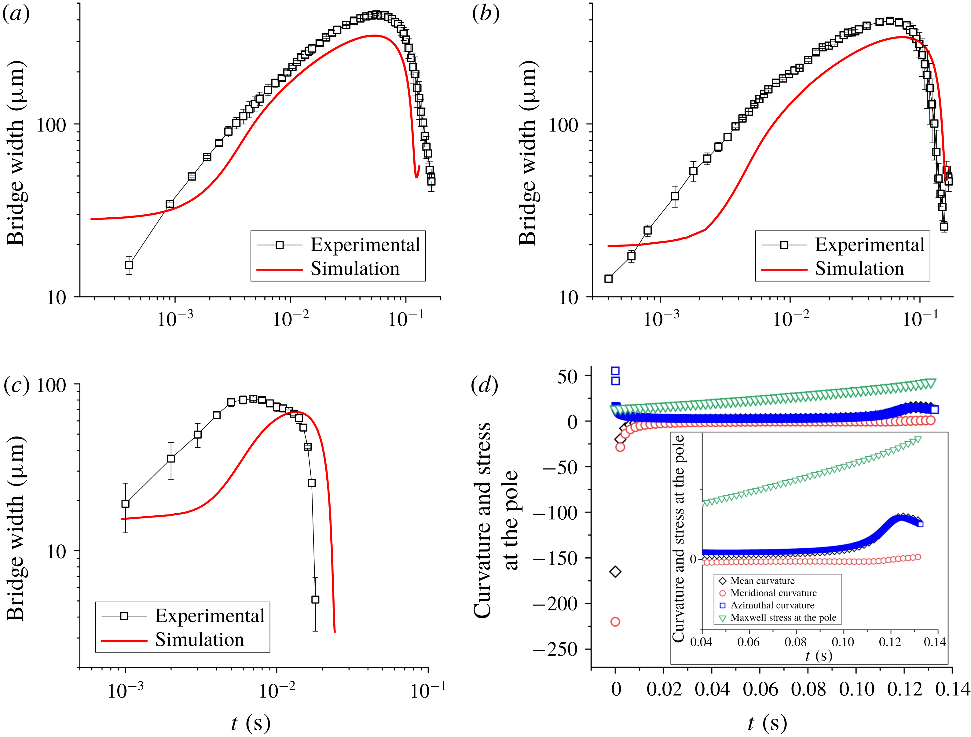
Figure 3(a) shows both experimental and numerical results of how the bridge between the connected droplets starts to widen with time as the droplets coalesce to form a larger drop. Experiments are repeated three times with similar initial conditions to obtain error bars as shown in figure 3(a). The disagreement between experiments and numerical simulation can be attributed to the exact dimension of the bridge on account of poor the resolution of the experimental images. The evolution of mean, meridional and azimuthal curvatures at the centre of the bridge is plotted in figure 3(b) to understand how the capillary pressure inside the bridge varies. 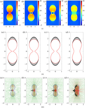As expected the mean curvature is negative at time $t=0$  s, favouring coalescence. The competition between azimuthal and meridional curvature determines whether the capillary pressure is positive or negative. In the case of the coalescing droplets, the strength of the electric field is low such that the azimuthal curvature soon falls to one and the meridional curvature rises to one, thereby forming a sphere. This phenomenon can be clearly observed in figure 4(i) which shows the pressure profile as the droplets coalesce, with negative pressure, on account of meridional curvature, favouring coalescence at the beginning and then the pressure equalizing throughout the drop at the end of coalescence process. The Maxwell stresses plotted in figure 4(ii) show that the free charges immediately redistribute at the poles with the stress acting only on the poles and not on the connected bridge. At low $Ca$ , the Maxwell stresses are not strong enough to pull the droplets apart and the negative meridional curvature remains high in the initial stages. Figure 4(iii) shows the streamlines and the velocity distribution along with interfacial velocities at various times during coalescence and, as evident from the plots, the direction of the velocity at the interface is outwards for all time steps, indicating coalescence.

Figure 3.

(a) Evolution of bridge with time for coalescence ( $Ca=0.063\pm 0.004$ and $Ca\approx 0$ ). (b) Curvatures at the centre of the bridge ( $Ca=0.063\pm 0.004$ ). (Inset: closer look at curvatures from time $t=0.08$  s to $t=0.24$  s.)

Figure 4.

(i) Pressure, (ii) Maxwell stress and (iii) velocity profiles ( $Ca=0.063$ ) at (a)  $t=0.00259$  s, (b)  $t=0.00518$  s, (c)  $t=0.00777$  s, (d)  $t=0.0259$  s. (The interfacial velocity has been plotted only for the left half of the connected droplets for clarity, and the colours are green for streamlines, red for quiver and black for interfacial velocity respectively.)

Figure 5.

Evolution of bridge with time for non-coalescence for (a)  $Ca=0.146\pm 0.005$ , (b)  $Ca=0.135\pm 0.007$ and (c)  $Ca=0.182\pm 0.002$ , and (d) curvatures at the centre of the bridge and stress at the poles ( $Ca=0.146$ ). (Inset: closer look at curvatures from time $t=0.04$ to $t=0.14$ .)

Figure 6.

(i) Pressure profiles, (ii) Maxwell stress profiles and (iii) velocity profiles ( $Ca=0.146$ ) for (a)  $t=0$  s, (b)  $t=0.008$  s, (c)  $t=0.009$  s, (d)  $t=0.011$  s, (e)  $t=0.019$  s, (f)  $t=0.026$  s, (g)  $t=0.094$  s, (h)  $t=0.121$  s, (i)  $t=0.127$  s, (j)  $t=0.13$  s. (In the velocity profiles the colours are green for streamlines, red for quiver and black for interfacial velocity.)

Figure 7.

(a) Bridge dynamics for a fixed initial bridge width for $Ca=0.182$ , $Ca=0.167$ and $Ca=0.154$ . (b) Initial bridge growth for $Ca=0.182$ , $Ca=0.167$ , $Ca=0.154$ , $Ca=0.143$ , $Ca=0.1$ , $Ca=0.08$ , $Ca=0.06$ , $Ca=0.04$ and $Ca=0.01$ . (c) Initial growth rate according to Eggers, Lister & Stone’s (Reference Eggers, Lister and Stone1999) model for $Ca=0.182$ , $Ca=0.167$ , $Ca=0.154$ , $Ca=0.143$ , $Ca=0.1$ , $Ca=0.08$ , $Ca=0.06$ , $Ca=0.04$ and $Ca=0.01$ . (d) Variation of transition time with $Ca$ . (e) Comparison of numerical and theoretical results of decay of bridge radius for $Ca=$ , $Ca=0.1666$ and $Ca=0.1538$ . (f) Collapse of decay plots for $Ca=0.182$ , $Ca=0.167$ , $Ca=0.154$ and $Ca=0.143$ .

On the contrary, when the strength of the electric field is increased, beyond a critical capillary number of 0.08 (Anand et al. Reference Anand, Roy, Naik, Juvekar and Thaokar2019), non-coalescence is observed. Figure 5(a) shows how the bridge evolves with time, reaching the peak value of $400~\unicode[STIX]{x03BC}\text{m}$ in the experiments and predicted as $320~\unicode[STIX]{x03BC}\text{m}$ in numerical simulation ( $3.5~\text{kV}~\text{cm}^{-1}$ , $Ca=0.146$ ), and finally starts to decrease, resulting in non-coalescence. Similar observations are reported here for two more capillary numbers ${>}0.1$ as shown in figures 5(b) and 5(c). All experiments were repeated three times using similar initial conditions to obtain error bars as shown in figures 5(a), 5(b) and 5(c). It stands to reason that the mean curvature at the centre and the total pressure should evolve and indicate why the bridge width increases (thereby favouring coalescence) and then decreases leading to non-coalescence. Figure 5(d) shows that at time $t=0$ the mean curvature at the centre is negative, indicating negative pressure and therefore liquid from the droplets starts to flow in and the mean curvature continues to be negative due to the dominance of the reduction in azimuthal curvature over the increase in meridional curvature, favouring coalescence. However the mean curvature starts to increase with time. As the value reaches $t=0.06$  s, the bridge starts to thin and at time $t=0.14$  s a singularity is reached, indicating code failure and breakup. Taking a closer look at the competing meridional and azimuthal curvatures, it is observed that the azimuthal curvature starts to dominate the meridional curvature beginning at time $t=0.1$  s and this dominance of azimuthal over meridional curvature leads to the mean curvature becoming positive at the centre, leading to non-coalescence.

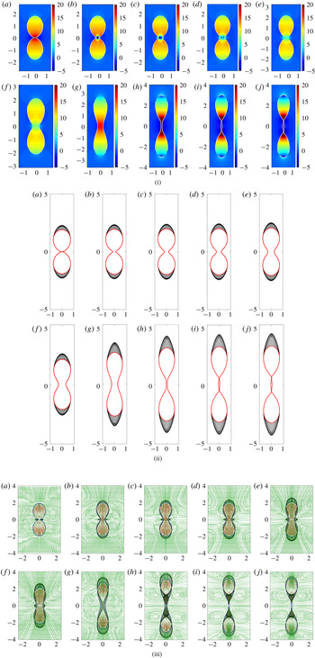
Similarly pressure profiles are also plotted indicating how the pressure at the centre varies (figure 6i). Initially negative at $t=0$  s to $t=0.009$  s (dimensional time), zero near $t=0.019$  s and positive beyond. The streamline and velocity profiles (figure 6iii) corroborate our observation and show how the interfacial velocity near the bridge is outwards initially (until $t=0.026$  s) favouring coalescence whereafter the direction reverses and turns inwards, indicating fluid moving outwards from the bridge towards the bulk.

Maxwell stresses (normal stresses) are also plotted as the drop evolves with time, as shown in figure 6(ii). It is seen that at time $t=0.12$  s the Maxwell stresses increase significantly, thereby reducing meridional curvature. Moreover the increased tensile Maxwell stresses at the poles reduce the pressure at the poles, thereby favouring non-coalescence, since the fluid flows from high pressure at the bridge towards the low pressure poles. The dominance of azimuthal curvature further aids non-coalescence.

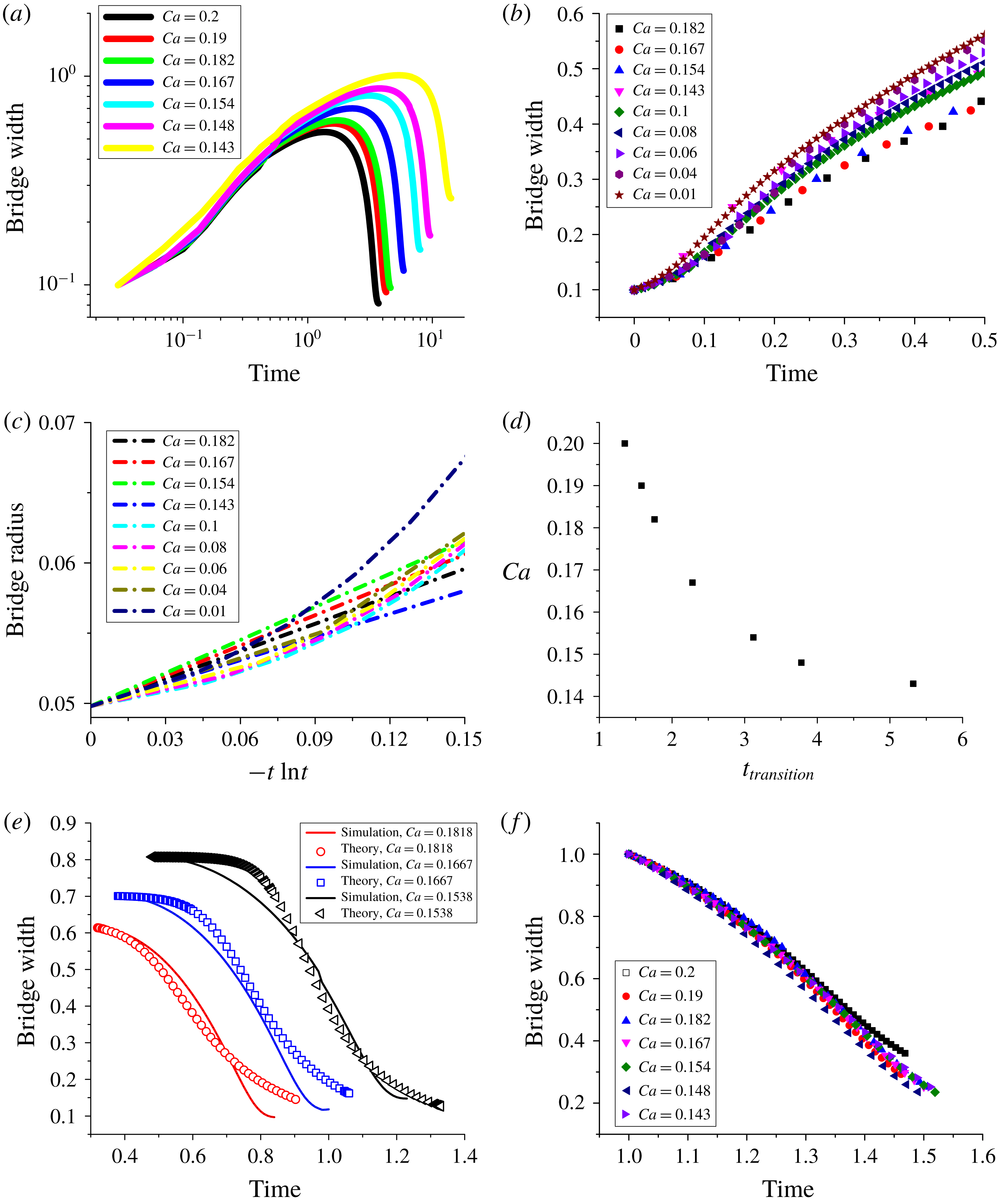
In the viscosity dominated regime, the coalescence of two droplets in the absence of an external electric field is a balance between the capillary force and the viscous force that leads to a linear relation between the growth of the bridge radius and time. On plotting the evolution of the bridge with time (non-dimensionalized using the viscous time scale ( $\unicode[STIX]{x1D707}a/\unicode[STIX]{x1D6FE}$ ) instead of the electric time scale) for various $Ca$ , it can be seen (figure 7 b) that during this growth phase the plots collapse, proving that the electric field or $Ca$ plays little or no part in determining how the bridge evolves. Eggers et al. (Reference Eggers, Lister and Stone1999) had shown that a logarithmic correction is required and the bridge radius grows as $r_{b}^{\ast }(t)=-(1/\unicode[STIX]{x03C0})t^{\ast }\ln (t^{\ast })$ , where $r_{b}^{\ast }=r_{b}/a$ , and $t^{\ast }=t/(\unicode[STIX]{x1D707}a/\unicode[STIX]{x1D6FE})$ . Here, $r_{b}(t)$ , $\unicode[STIX]{x1D6FE}$ , $t$ , $\unicode[STIX]{x1D707}$ and $a$ are bridge radius, interfacial tension, time, viscosity of the drop and initial drop radius respectively, and all symbols with $\ast$ are dimensionless. In figure 7(a) simulation results of the evolution of the bridge diameter are plotted for different $Ca$ values. The initial growth rates for different $Ca$ as well as for $Ca\approx 0$ are plotted according to Eggers et al.’s (Reference Eggers, Lister and Stone1999) model in figure 7(c). While the plots are linear in nature to indicate the model is valid, this is only applicable for a very short time. The slope is found to be slightly higher than $1/\unicode[STIX]{x03C0}$ . At longer times, the rate of bridge growth decreases with $Ca$ due to negative pressure at the poles.

Another interesting observation from these plots is the variation of the transition time ( $t_{t}$ ) (the point in the evolution of the bridge when the bridge stops growing, reaches a peak value and thereafter starts to shrink) with $Ca$ . Figure 7(d) shows that $Ca$ is inversely proportional to  $t_{t}$ . In this regime, the Maxwell stress is strong enough to stretch the connected droplets, thereby countering the flow of liquid from the bulk to the bridge.

On the other hand, the decay of the bridge width can be modelled as a viscous squeezing flow out of the bridge due to differences between the bridge pressure and the pressure in the bulk of the drop. This leads to $\text{d}d_{b}^{\ast }/\text{d}t^{\ast }=-\frac{1}{64}(d_{b}^{\ast 3}/L^{\ast 2})[a_{1}(2/d_{b}^{\ast })-(2-a_{2}(Ca/2))]$ where $d_{b}^{\ast }=d_{b}/a$ , $t^{\ast }=t/(\unicode[STIX]{x1D707}a/\unicode[STIX]{x1D6FE})$ and $L^{\ast }=L/a$ . Here, $d_{b}$ and $L$ are the bridge width and length of the bridge respectively. However the model does not take into account (i) that the meridional curvature retards the squeezing action, and (ii) that the electric stress is higher at the poles of the droplets when compared to a spherical droplet. Thus $a_{1}$ and $a_{2}$ are introduced to adjust these two terms (e.g. for $Ca=0.182$ , $a_{1}=0.45$ and $a_{2}=6.3$ ), and a reasonable agreement is observed between the model and simulation results. The results are shown in figure 7(e).

The decay regimes of these bridge evolutions can also be made to collapse, thereby showing that $Ca$ only affects the time at which the direction of bridge evolution reverses (figure 7 f). Therefore it is seen that both rates of growth and decay are linear in nature and independent of  $Ca$ .