





1. Introduction
Wave breaking has been experimentally observed in highly viscous vertical falling liquid films, where it generates large liquid ligaments that detach from the free surface (Gourdon et al. Reference Gourdon, Innings, Jongsma and Vamling2015). Representative examples are shown in figure 1, which presents photographs from Gourdon et al. (Reference Gourdon, Innings, Jongsma and Vamling2015) of concentrated milk falling on the outside of an evaporator tube at relatively high dry solids content (
 $\geqslant 45\,\%$
) and correspondingly high viscosities. Such events also promote undesirable bubble entrainment, and contribute to the formation of large vapour bubbles, foams or even dry patches in falling film evaporators (Johansson et al. Reference Johansson, Leifer, Vamling and Olausson2009; Doro Reference Doro2012). These phenomena are particularly relevant in industrial evaporators that involve highly viscous non-Newtonian liquids, such as milk at high dry solid content, where shear-thinning and yield stress significantly alter wave dynamics (Gourdon et al. Reference Gourdon, Innings, Jongsma and Vamling2015). Additionally, liquid ligament detachment broadens the residence time distribution in the evaporator, impairing control of temperature exposure and local concentrations. Note that figure 1 illustrates the phenomenon and its industrial significance, but it does not serve as a quantitative reference case for the present study, which focuses on the onset of wave breaking that leads to these phenomena.
Wave breaking has been extensively studied in the context of ocean waves, where it plays a central role in air–sea interactions, energy dissipation, momentum transfer and bubble entrainment (Banner & Peregrine Reference Banner and Peregrine1993; Melville Reference Melville1996; Banner & Peirson Reference Banner and Peirson2007; Perlin et al. Reference Perlin, Choi and Tian2013; Mostert et al. Reference Mostert, Popinet and Deike2022). In that setting, breaking is driven by the steepening of gravity waves when the orbital velocity of water particles at the crest exceeds the wave phase speed, causing the crest to overturn. Surface tension plays a negligible role at the length scales relevant to ocean waves, and the breaking criterion is governed by the competition between inertia and gravity, commonly expressed via a wave steepness threshold. In highly viscous vertical falling liquid films, however, the physical picture is fundamentally different. Here, the relevant length scales are of the order of the film thickness (typically
 $\mathcal{O}(1)$
mm), and the surface tension plays a central role in arresting the steepening of the wave front.
Even at moderate flow rates, initially flat vertical films become unstable to the Kapitza instability, inducing surface waves whose growth is driven by inertia in the gravity-driven primary flow (Kapitza & Kapitza Reference Kapitza and Kapitza1949). The onset and evolution of these waves have been extensively studied, particularly for Newtonian liquids, establishing a detailed understanding of the wave dynamics (Kalliadasis et al. Reference Kalliadasis, Ruyer-Quil, Scheid and Velarde2012).
On the other hand, wave breaking in vertical falling liquid films, when the front of a wave overturns and the wave disintegrates, has been addressed in markedly few studies. Joo et al. (Reference Joo, Davis and Bankoff1991) reported that this phenomenon is associated with the breakdown of numerical solutions to the Benney equation (Benney Reference Benney1966), an evolution equation obtained by asymptotic expansion in terms of the long-wave parameter around the primary flow solution. Gjevik (Reference Gjevik1970) augmented the long-wave equation by retaining capillary effects. Formally, this is only valid in the limit of large enough Kapitza number values. Yet the author showed that this effect is essential for capturing the saturation mechanism of Kapitza waves on falling liquid films. This presages the role of surface tension in maintaining non-breaking travelling-wave solutions (TWS). According to Joo et al. (Reference Joo, Davis and Bankoff1991), wave breaking is caused by the difference in celerity between wave hump, initially faster, and wave trough, initially slower, during the linear and nonlinear growth phases of the Kapitza instability. The surface-tension-driven adaptation of these disparate celerities during the nonlinear saturation of a Kapitza wave is associated with a distortion of the wave front (Dietze Reference Dietze2016), which at some point can no longer be captured with the Benney equation. Indeed, low-dimensional models of this type require the film thickness to be a single-valued function of the streamwise coordinate, which precludes the study of overhanging wave profiles. Ruyer-Quil et al. (Reference Ruyer-Quil, Chakraborty and Dandapat2012) mentioned wave-breaking events that occurred in some of their multiphase direct numerical simulations (DNS) of falling films of a power-law liquid (for large wavelengths), but such results were not shown in their paper. Finally, when analysing the asymmetry of solitary waves, Denner et al. (Reference Denner, Pradas, Charogiannis, Markides, van Wachem and Kalliadasis2016) mention that wave breaking is possible if the inertia and inclination angle are sufficiently high to overcome the opposing effect of surface tension, and Doro (Reference Doro2012) stated that wave breaking can be triggered by transient phenomena, such as wave coalescence.
Concentrated milk falling on the outside of an evaporator tube, illustrating wave breaking and liquid ligament detachment from the free surface: (a) 45 % dry solids (DS) content at
 $\textit{Re}_\varGamma =22$
,
 $\textit{Ka}=15$
, during evaporation; (b) 50 % DS at
 $\textit{Re}_\varGamma =18$
,
 $\textit{Ka}=7$
, during evaporation; (c,d) 50 % DS without evaporation at 0.3 m and 1.5 m from the inlet, respectively. (The parameters
 $\textit{Re}_\varGamma$
and
 $\textit{Ka}$
are defined in § 2.1; for the 50 % DS milk these correspond approximately to point
 $B$
in figure 13.) The images capture post-breaking dynamics, including three-dimensional ligament detachment, which is outside the scope of the present two-dimensional study that targets the onset of breaking rather than the subsequent post-breaking regime. Note also that the conditions shown are local to specific positions along the evaporator tube and are not representative of the full tube height, where the flow regime and fluid properties vary continuously. Reprinted from Gourdon et al. (Reference Gourdon, Innings, Jongsma and Vamling2015), with permission from Elsevier.

In this work, we investigate the onset of wave breaking in vertical falling films via multiphase DNS, and identify the governing parameters. We characterise this phenomenon as a loss of TWS, i.e. the loss of a dynamic equilibrium state, rather than as the emergence of an additional instability or transient mechanism. We examine how gravitational, viscous and capillary effects control this transition, and map the corresponding parameter regimes. We consider both Newtonian and Herschel–Bulkley liquids, and show that yield stress and shear-thinning modify wave morphology, internal flow, and the propensity for wave breaking. Furthermore, we report the existence of overhanging TWS, which represent a previously unrecognised intermediate state between standard TWS and wave breaking. Such overhanging wave profiles are inherently inaccessible to low-dimensional models, which require the film thickness to be a single-valued function of the streamwise coordinate, and have therefore, to the best of our knowledge, not been reported in previous studies of falling film dynamics. The post-breaking dynamics, including bubble entrainment and liquid ligament detachment as observed experimentally in figure 1, is inherently three-dimensional and falls outside the scope of the present study. We are interested in the preceding two-dimensional phenomena.
Our results are presented in terms of key dimensionless parameters, providing a framework for understanding wave breaking across a wide range of operating conditions and Newtonian and viscoplastic/shear-thinning liquids that can be represented by the Herschel–Bulkley model. The findings extend classical Kapitza wave descriptions of falling film dynamics, and identify critical conditions for breaking, with implications for predicting and controlling heat and mass transfer, film integrity, bubble entrainment and liquid residence time in Newtonian and non-Newtonian systems.
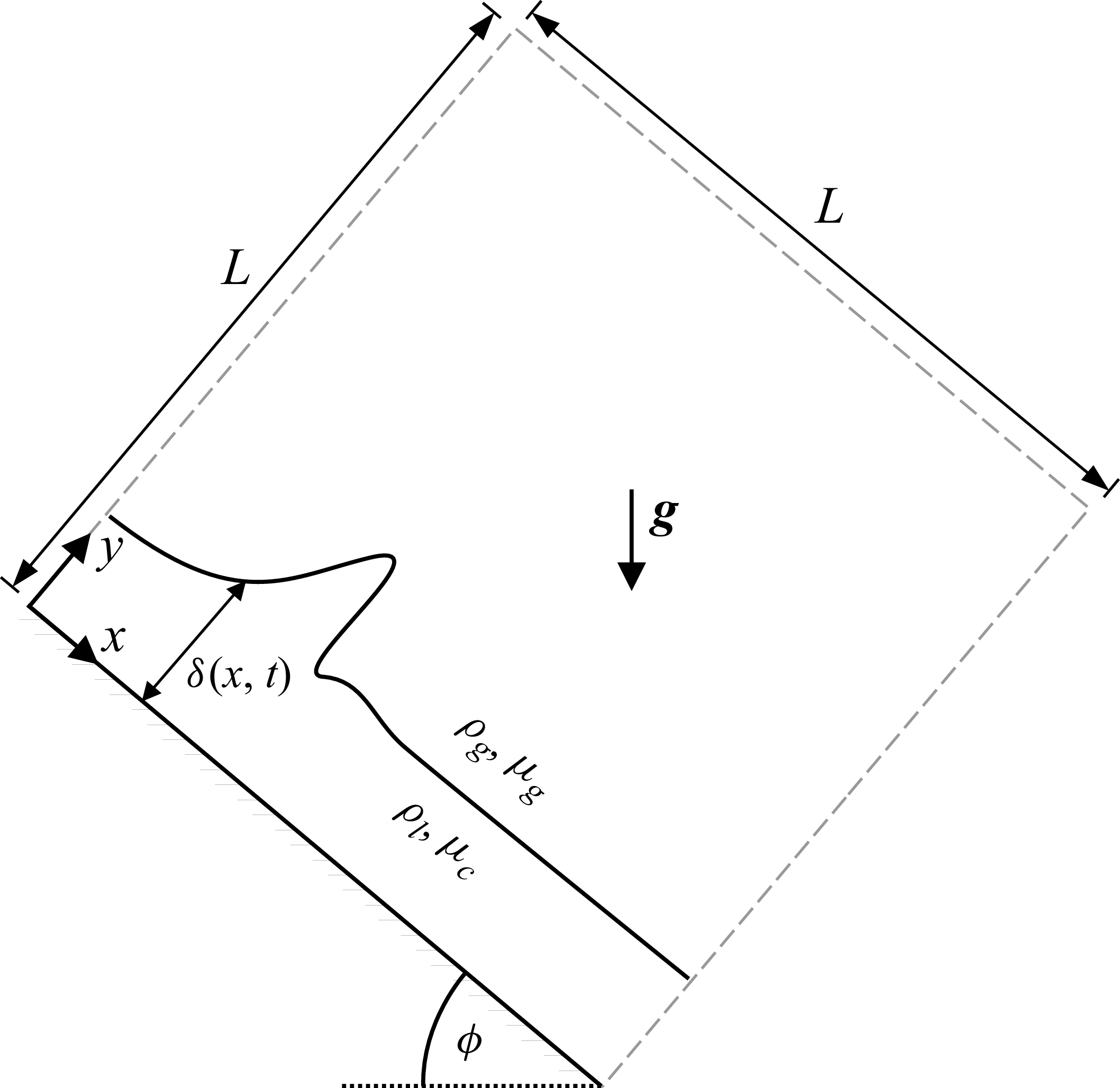
Schematic of the problem and our computational domain: a Newtonian or viscoplastic film flows down a smooth plane inclined at angle
 $\phi$
. In this work, we focus on vertical falling films where
 $\phi =90^\circ$
, except for the validation case in § 3.3. The computational domain is a square of length
 $L$
with periodic boundary conditions at
 $x=(0,L)$
(except in § 3.3), no-slip at
 $y=0$
, and symmetry at
 $y=L$
. Here,
 $\delta (x,t)$
is the local film thickness, while
 $\delta$
denotes the mean film thickness.

2. Governing equations and numerical approach
We study, using two-dimensional multiphase DNS, liquid films flowing down a smooth wall inclined at an angle
 $\phi$
from the horizontal plane under the effect of gravity. Positive
 $x$
and
 $y$
denote the streamwise (tangential) and wall-normal directions, respectively. Figure 2 shows a schematic of the problem, and illustrates our periodic computational domain. Except for the validation case in § 3.3, this work is limited to vertical falling films where
 $\phi =90^\circ$
. We consider both Newtonian and non-Newtonian liquids described by a generalised Newtonian (Herschel–Bulkley) model formulated in terms of an effective viscosity as
 \begin{align} \begin{cases} \mu = K\gamma ^{n-1} + \dfrac {\tau _y}{\gamma } & \textrm{if} \ \tau \geqslant \tau _y, \\[9pt] \gamma _{ij} = 0 & \textrm{if} \ \tau \lt \tau _y . \end{cases} \end{align}
Here,
 $K$
,
 $n$
and
 $\tau _y$
are the consistency, power-law index and yield stress, respectively. The deviatoric stress components are
 $\tau _{ij}=\mu \gamma _{ij}$
, with
 $\gamma _{ij}=(\partial _ju_i+\partial _iu_j)$
, where
 $\partial _i$
is a spatial derivative. The extra-stress intensity is defined as
 $\tau =\sqrt {0.5\sum _{i,j}\tau _{ij}\tau _{ji}}$
(where
 $\tau \sqrt {2}$
equals the Frobenius norm), and the strain rate is
 $\gamma =\sqrt {0.5\sum _{i,j}\gamma _{ij}\gamma _{ji}}$
(Balmforth & Liu Reference Balmforth and Liu2004). Specifying
 $n=1$
and
 $\tau _y=0$
thus recovers Newtonian behaviour. Numerically, the main difficulty arises from the yield condition: the material flows for
 $\tau \gt \tau _y$
, but behaves as a solid (
 $\gamma =0$
) otherwise, which implies that
 $\mu \to \infty$
as
 $\gamma \to 0$
in (2.1) (Balmforth et al. Reference Balmforth, Frigaard and Ovarlez2014). To avoid this singularity, we use a regularised formulation with an effective viscosity
 $\mu _l$
given by
 \begin{equation} \mu _l = \min (K\gamma ^{n-1} + \tau _y/\gamma , \mu _{\textit{max}}) , \end{equation}
where
 $\mu _{\textit{max}}$
is the regularisation parameter, which we have chosen based on careful sensitivity analyses in § 3.
2.1. Dimensionless numerical framework
We non-dimensionalise all variables using the liquid density
 $\rho _l$
, mean film thickness
 $\delta$
, and characteristic velocity
 \begin{equation} V_c=\delta \left (\dfrac {\rho _l g \delta \sin \phi -\tau _y}{K}\right )^{1/n}, \end{equation}
defined from a balance between gravitational and viscous stresses,
 $\rho _l \delta g \sin \phi = \tau _c$
. This gives the characteristic shear rate
 $\gamma _c=V_c/\delta$
, shear stress
 $\tau _c=\mu _c\gamma _c=K\gamma _c^n+\tau _y$
and effective viscosity
 $\mu _c=K\gamma _c^{\,n-1}+\tau _y/\gamma _c$
, which accounts for the yield stress contribution, consistent with recommendations by Thompson & Soares (Reference Thompson and Soares2016). For a flat film in a passive gas,
 $\tau _c$
is the wall shear stress; hence
 $\mu _c$
and
 $\gamma _c$
are wall-based quantities, and
 $V_c$
is a characteristic velocity derived from the wall shear rate.
The non-dimensional variables are the spatial coordinates
 $x^*_i = x_i/\delta$
, velocity
 $u^*_i = u_i / V_c$
, time
 $t^*= t/(\delta / V_c)$
, shear rate
 $\gamma _{ij}^*=\gamma _{ij}\delta /V_c$
, density
 $\rho ^* = \rho /\rho _l$
, dynamic viscosity
 $\mu ^* = \mu /\mu _c$
, pressure
 $p^* = p/(\rho _l V_c^2 )$
, interface curvature
 $\kappa ^* = \kappa \delta$
, and the Dirac distribution function
 $\delta _S^*=\delta _S \delta$
. The non-dimensional governing equations read
 \begin{align} \boldsymbol{\nabla }\boldsymbol{\cdot } \boldsymbol{u}^* = 0, \end{align}
 \begin{align} \textit{Re}_c {\rho ^*}\dfrac {{\rm D}{\boldsymbol{u}^*}}{{\rm D}t^*} = -\textit{Re}_c\boldsymbol{\nabla }\!p^* + \boldsymbol{\nabla }\boldsymbol{\cdot }({\mu ^*}\boldsymbol{\gamma }^*) + \dfrac {{\boldsymbol{g}^{*}}{\rho^*}}{\sin \phi } + \dfrac {{\kappa ^*}{\delta_S^*}\hat {\boldsymbol{n}}}{\textit{Eo}} , \end{align}
 \begin{align} \dfrac {\partial f}{\partial t^*} + \boldsymbol{\nabla }\boldsymbol{\cdot } (\boldsymbol{u}^* f) = 0, \end{align}
where
 $\boldsymbol{g}^*=\sin \phi \,\boldsymbol{e}_x-\cos \phi \,\boldsymbol{e}_y$
is the gravitational acceleration vector,
 $\boldsymbol{e}_x$
and
 $\boldsymbol{e}_y$
are unit vectors,
 $\hat {\boldsymbol{n}}$
is the interface normal, and
 $f$
is the volume fraction (
 $f=1$
in the liquid,
 $f=0$
in the gas). In periodic domains, gravity is applied only in the liquid phase to prevent spurious gas acceleration. The fluid properties in (2.4)–(2.6) are computed as
 \begin{align} &\rho ^*=f+(1-f)\rho _r, \\[-12pt]\nonumber \end{align}
 \begin{align} &\begin{cases} \mu ^*=f\kern-0.5pt\mu ^{*}_l+(1-f)\mu _r,\\[5pt] \mu ^{*}_l= \mu _l / \mu _c = \min [(1-\textit{Pl}){\gamma ^*}^{n-1} + \textit{Pl}/{\gamma ^*}, \mu ^*_{\textit{max}}]. \end{cases} \end{align}
From these governing equations, we obtain the dimensionless governing parameters
 \begin{equation} \textit{Re}_c = \dfrac {\rho _l V_c \delta }{\mu _c}, \quad \textit{Eo} = \dfrac { \rho _l g \delta ^2 \sin \phi }{\sigma },\quad \textit{Pl} = \dfrac {\tau _y}{\rho _l g \delta \sin \phi },\quad \rho _r = \dfrac {\rho _g}{\rho _l},\quad \mu _r = \dfrac {\mu _g}{\mu _c},\quad n, \quad\phi \end{equation}
that fully describe the present problem, where
 $\sigma$
is the surface-tension coefficient. The characteristic Reynolds number
 $\textit{Re}_c$
quantifies inertial relative to viscous forces, while the Eötvös number
 $\textit{Eo}$
relates gravity to surface tension. The plasticity number
 $\textit{Pl} \in [0,1]$
indicates the fraction of the primary flow that is unyielded, with
 $0$
for Newtonian, and
 $1$
for fully unyielded (Thompson & Soares Reference Thompson and Soares2016).
We fix
 $\rho _r = \mu _r = 0.001$
, which represents industrially relevant and highly viscous values, and implies negligible gas stresses (Kalliadasis et al. Reference Kalliadasis, Ruyer-Quil, Scheid and Velarde2012). We further assume quiescent, practically unconfined, gas conditions. The influence of the gas on the liquid phase is thus negligible, and the exact values of
 $\rho _r$
and
 $\mu _r$
do not significantly influence our results. With
 $\rho _r$
,
 $\mu _r$
fixed, the governing parameters
 $(\textit{Re}_c,\textit{Eo}, \textit{Pl}, n)$
therefore completely describe the film dynamics for a given
 $\phi$
. The values used for these parameters in our simulations also represent realistic and industrially relevant conditions, as discussed in § 4.3. At some points, we use the Reynolds number based on the wetting rate
 $\varGamma$
(mass flow rate per unit width),
 $\textit{Re}_{\varGamma } = \varGamma /\mu _c = \rho _l V \delta /\mu _c$
, where
 $V$
is the mean vertical film velocity. In inlet–outlet domains,
 $\textit{Re}_{\varGamma }$
prescribes the inlet mass flow, with film thickness and velocity as outputs. In periodic domains, the film thickness is fixed, and
 $\textit{Re}_{\varGamma }$
is an output.
We also note the following relations to other dimensionless groups frequently used in falling film analysis: the Froude number as
 $\textit{Re}_c \sin \phi = Fr^2 = V_c^2/(g\delta )$
, the Weber number
 $\textit{We}=\rho _l \delta V_c^2/\sigma = \textit{Re}_c \textit{Eo}$
, and the Kapitza number
 $\textit{Ka} = \sigma \rho ^{1/3}/((g\sin \phi )^{1/3}\mu _c^{4/3}) = \textit{Re}_c^{2/3}/\textit{Eo}$
. Note that these relations are given here for convenience, and that in the present study, we mainly focus on the governing parameters defined in (2.9).
The simulation domain is always a square with length
 $L$
with no-slip boundary conditions (
 $u=v=0$
) at the wall. For all cases in § 4, we use periodic boundaries in the streamwise direction, and domain of length
 $L=40\delta$
. We initialise a film of mean thickness
 $\delta$
perturbed with a sinusoid of wavelength
 $L$
and amplitude
 $0.1\delta$
that allows us to study finite-amplitude travelling wave solutions (TWS) and their transition to wave-breaking states. For high yield stress (
 $\textit{Pl}=0.5$
) and low Reynolds number (
 $\textit{Re}_c\leqslant 7.2$
),
 $L=40\delta$
is below the cut-off wavelength for the Kapitza instability, so we use here
 $L=80\delta$
in these cases, in order to accommodate longer waves. Limiting the domain to one wavelength isolates a mode close to the most-amplified mode while maintaining numerical efficiency for the parametric study in § 4.3. The TWS simulations typically reach a statistical steady state by
 $t^* \sim \mathcal{O}(100)$
in periodic domains. The film grid spacing and the regularisation parameter are fixed at
 $\varDelta =\delta /51$
and
 $\mu ^*_{\textit{max}}=500$
. These parameters are determined via sensitivity studies presented in §§ 3.1 and 3.2, with validation against experiments in § 3.3.
The simulations are performed using the open-source code Basilisk (Popinet Reference Popinet2015), which has been used for simulating different liquid film flows (Lavalle et al. Reference Lavalle, Mergui, Grenier and Dietze2021; Choudhury et al. Reference Choudhury, Filoche, Ribe, Grenier and Dietze2023; Hidman et al. Reference Hidman, Åkesjö, Gourdon, Jongsma, Ström, Sardina and Sasic2024). A cell-centred Cartesian adaptive grid is used, with uniform maximum resolution in the liquid, and gradual coarsening in the gas to grid spacing
 $\varDelta =L/64$
. The equations are solved using a projection method with second-order time integration, standard second-order spatial discretisation, and Bell–Colella–Glaz advection for velocity. The interface treatment involves a VOF–PLIC scheme (Scardovelli & Zaleski Reference Scardovelli and Zaleski1999) with geometric advection, height-function curvature, and a well-balanced surface-tension formulation (Popinet Reference Popinet2018). The viscoplastic viscosity model is applied in the liquid, while the gas properties are constant.
The present study employs two-dimensional simulations, which are well suited to capture the wave dynamics up to and including the onset of breaking. The pre-breaking processes, including wave growth and steepening, the formation of overhanging TWS, and the breakdown of the capillary–gravitational force balance, are expected to be essentially two-dimensional in nature, consistent with previous studies in falling liquid films showing that three-dimensional effects emerge only after the saturation of two-dimensional surface waves (Chang et al. Reference Chang1994; Kofman et al. Reference Kofman, Mergui and Ruyer-Quil2014), which can be considered a consequence of the Squire theorem that is known to apply to Newtonian falling liquid films (Yih Reference Yih1955). For the viscoplastic cases, the high effective viscosity observed in the wave hump (see e.g. figure 10 below) further suggests that the growth rate of a three-dimensional accelerational Rayleigh–Taylor mode (Kofman et al. Reference Kofman, Mergui and Ruyer-Quil2014) on the wave crest would be weak relative to the rate of breaking. Three-dimensional effects are expected to become important primarily in the post-breaking regime, where the overturning wave front is subject to the full measure of gravity and becomes infinitely steep, leading to an increased growth rate of the spanwise Rayleigh–Taylor instability mode, and subsequent ligament formation and break-up. The three-dimensional post-breaking dynamics is outside the scope of the present work. Rather, we are interested in the two-dimensional dynamics of the liquid film leading up to wave breaking. One outcome of our study is that wave breaking is preceded by overhanging TWS, which represent an excellent starting point to study the three-dimensional disintegration of Kapitza waves into liquid ligaments, via linear stability analysis in future work.
3. Validation
To ensure accurate simulations for Herschel–Bulkley liquids, we first determine suitable film grid spacing and regularisation parameter
 $\mu _{\textit{max}}$
by comparison to analytical solutions for viscoplastic vertical flat films and sensitivity studies focused on the nonlinear wave shape at the wave-breaking onset. Then we further validate the numerical method by reproducing the viscoplastic wavy falling film experiments of Mounkaila Noma et al. (Reference Mounkaila Noma, Dagois-Bohy, Millet, Ben Hadid, Botton and Henry2023) on inclined surfaces.
3.1. Validation against analytical solution for flat vertical film
We consider a viscoplastic flat film flowing down a smooth vertical wall (
 $y^*=0$
) in the
 $x^*$
direction, with the free surface at
 $y^*=1$
. For non-zero yield stress (
 $\textit{Pl}\gt 0$
), the equilibrium consists of a shearing layer at the wall beneath a rigid plug, separated by a yield surface at
 $y^*=1-\textit{Pl}$
, where
 $\tau ^* = \textit{Pl}$
(Balmforth & Liu Reference Balmforth and Liu2004). Assuming no-slip at the wall,
 $u^*(0)=0$
, and stress-free at the interface,
 $\tau ^*_{xy}(y^*=1)=0$
, the momentum balance reduces to
 $\partial _y^* \tau ^*_{xy} = 1$
. Using the constitutive relation
 $\tau ^*_{xy} = \mu _l^*\gamma ^*_{xy} = -[(1-\textit{Pl})\,|\partial _y^* u^*|^n + \textit{Pl}]$
and integrating twice with the boundary conditions yields the vertical velocity profile
 \begin{equation} u^*(y^* ) = \begin{cases} (1-\textit{Pl})\left [1 -\left (\dfrac {Pl+y-1}{Pl-1}\right )^{1+1/n}\right ]\dfrac {n}{n+1} \ &\forall\ 0 \leqslant y^* \leqslant 1-\textit{Pl} , \\[25pt] (1-\textit{Pl})\dfrac {n}{n+1}&\forall \ 1-\textit{Pl} \lt y^* \leqslant 1 . \end{cases} \end{equation}
The mean vertical velocity of the flat film,
 $V_0^*=\int _{y^*=0}^{y^*=1}u^*(y^*)\,\text{d}y^*$
, then becomes (similarly to that obtained by de Freitas Maciel et al. (Reference de Freitas Maciel, de Oliveira Ferreira and Fiorot2013) and de Oliveira Ferreira et al. (Reference de Oliveira Ferreira, Maciel and Pereira2021))
 $V_0^* = (1-\textit{Pl})(({n+1+n\textit{Pl}})/({2n+1}))( {n}/({n+1}))$
. For Newtonian fluids (
 $n=1$
,
 $\textit{Pl}=0$
),
 $V_0^* = V_0/V_c = 1/3$
. In general,
 $V_0^*$
decreases with
 $n$
and increasing
 $\textit{Pl}$
, reaching
 $V_0^* \approx 0.15$
at
 $n=0.5$
and
 $\textit{Pl}=0.5$
.
For
 $\textit{Pl}=0.2$
and
 $n=0.6$
(a shear-thinning yield-stress liquid representative of our wavy falling films in § 4), comparison of our simulations for a flat film in a periodic domain with the analytical solution (3.1) shows good agreement at
 $\mu ^*_{\textit{max}}=500$
using the grid spacing
 $\varDelta =\delta /40$
(figure 3
a). This resolution represents a suitable balance between accuracy and computational cost.
Using
 $\varDelta =\delta /40$
, figure 3(b) shows that
 $\gamma ^*$
approaches but never equals zero at
 $y^*\gt 1-\textit{Pl}=0.8$
. This is due to the regularisation approach, where
 $\mu ^*_{\textit{max}}$
is finite and the plug region always exhibits a small but non-zero shear. Still, a value
 $\mu ^*_{\textit{max}}=500$
yields practically converged results, satisfactorily captures plug behaviour, and avoids excessive numerical stiffness; it is therefore adopted throughout this work.
Validation against the analytical solution (3.1) for a vertical flat film (
 $\textit{Pl}=0.2$
and
 $n=0.6$
, shear-thinning viscoplastic fluid). (a) Velocity profiles show that
 $\varDelta =\delta /40$
provides satisfactory grid convergence. (b) Influence of the regularisation parameter
 $\mu _{\textit{max}}$
on the strain rate using this resolution;
 $\mu ^*_{\textit{max}}=500$
adequately captures plug behaviour without excessive numerical stiffness.

3.2. Sensitivity of numerical parameters on wave dynamics at wave-breaking onset
To further justify our choices of numerical parameters, we perform additional sensitivity studies examining how the grid spacing
 $\varDelta$
and regularisation parameter
 $\mu _{\textit{max}}$
affect the wave dynamics at conditions close to and at the onset of wave breaking. For this, we select some of the solutions that will be discussed in § 4.3. We choose two representative cases at
 $\textit{Re}_c=13.9$
,
 $\textit{Pl}=0.5$
,
 $n=0.7$
: one with
 $\textit{Eo}=1.81$
, which yields a steady overhanging TWS, and one with
 $\textit{Eo}=2.77$
, which gives a breaking wave solution. The chosen parameter set exhibits representative breaking wave dynamics, a high yield stress, and significant shear-thinning effects.
We start by fixing the regularisation parameter to
 $\mu _{\textit{max}}^*=500$
based on the sensitivity studies in § 3.1, and vary the grid spacing as
 $\varDelta =\delta /25$
,
 $\delta /51$
and
 $\delta /102$
. Results for conditions close to the onset of wave breaking (
 $\textit{Eo}=1.81$
, steady overhanging TWS) and within the wave-breaking regime (
 $\textit{Eo}=2.77$
) are shown in figure 4. The solutions obtained with
 $\varDelta =\delta /51$
and
 $\varDelta =\delta /102$
are in close agreement for both cases, confirming that
 $\varDelta =\delta /51$
is sufficient for the present study.
We next assess the influence of the regularisation parameter on the wave dynamics for the same two cases, fixing the grid resolution to
 $\varDelta =\delta /51$
, and varying
 $\mu _{\textit{max}}^*=\mu _{\textit{max}}/\mu _c \in \{10, 100, 500, 1000\}$
. Figure 5 shows the predicted wave shapes at conditions close to the onset of wave breaking (
 $\textit{Eo}=1.81$
, steady overhanging TWS) and within the wave-breaking regime (
 $\textit{Eo}=2.77$
). The results indicate that
 $\mu _{\textit{max}}^*\lesssim 100$
noticeably affects the wave dynamics, whereas
 $\mu _{\textit{max}}^*\gtrsim 500$
yields solutions that are practically insensitive to this parameter. Taken together, these sensitivity studies confirm that the chosen numerical parameters
 $\varDelta =\delta /51$
and
 $\mu _{\textit{max}}^*=500$
produce wave dynamics that is robust with respect to both the grid resolution and the regularisation parameter.
Influence of grid resolution
 $\varDelta \in \{\delta /25, \delta /51, \delta /102\}$
on the instantaneous wave shape, effective viscosity field
 $\mu _l^*$
, and yield surface
 $\tau ^*=\textit{Pl}$
(white lines) for
 $\textit{Re}_c=13.9$
,
 $\textit{Pl}=0.5$
,
 $n=0.7$
at
 $\mu _{\textit{max}}^*=500$
. (a) For
 $\textit{Eo}=1.81$
, snapshot at
 $t^*=200$
: the coarsest grid predicts wave breaking, whereas the two finer resolutions saturate to an overhanging TWS. (b) For
 $\textit{Eo}=2.77$
, snapshot at
 $t^*=190$
: all resolutions predict a breaking wave solution. These results confirm that
 $\varDelta =\delta /51$
is sufficient for capturing the wave dynamics at conditions close to the onset of wave breaking.

Influence of the regularisation parameter
 $\mu _{\textit{max}}^*=\mu _{\textit{max}}/\mu _c \in \{10, 100, 500, 1000\}$
on the instantaneous wave shape, effective viscosity field
 $\mu _l^*$
, and yield surface
 $\tau ^*=\textit{Pl}$
(white lines) for
 $\textit{Re}_c=13.9$
,
 $\textit{Pl}=0.5$
,
 $n=0.7$
at grid resolution
 $\varDelta =\delta /51$
. (a) For
 $\textit{Eo}=1.81$
, snapshot at
 $t^*=200$
: the lowest
 $\mu _{\textit{max}}^*$
produces a significantly smaller wave hump, whereas
 $\mu _{\textit{max}}^*\gtrsim 500$
yields a practically converged solution. (b) For
 $\textit{Eo}=2.77$
, snapshot at
 $t^*=180$
:
 $\mu _{\textit{max}}^*=500$
again yields essentially converged results for the breaking wave case. The thickening ahead of the main wave is a secondary wave developing in its tail, which the faster main wave nearly catches up with before breaking.

Comparison of our simulations with experiments by Mounkaila Noma et al. (Reference Mounkaila Noma, Dagois-Bohy, Millet, Ben Hadid, Botton and Henry2023) for a viscoplastic film (
 $\textit{Pl}=0.12,\ n=0.53$
) flowing down a
 ${2}\ \mathrm{m}$
channel at
 $\phi =13.9^\circ$
, with inlet perturbation
 $\omega ={1.5}\,\mathrm{Hz}$
. (a) Wave amplitude
 $A(x)$
sampled every
 ${10}\ \mathrm{cm}$
along the channel. (b) Instantaneous film height
 $\delta (x,t)$
at
 $x=-90$
,
 $-50$
and
 $-{10}\ \mathrm{cm}$
from the outlet (orange crosses in (a)).

3.3. Validation with experiments in a wavy viscoplastic film on an inclined plane
We further validate the method by simulating roll waves in a viscoplastic film on an inclined plane, reproducing the experiments reported in Mounkaila Noma et al. (Reference Mounkaila Noma, Dagois-Bohy, Millet, Ben Hadid, Botton and Henry2023) (figures 2a,b). A Carbopol film flows down a
 $2\ \mathrm{m}$
long,
 $0.5\ \mathrm{m}$
wide channel at
 $\phi =13.9^\circ$
, corresponding to
 $\textit{Re}_c=10.6$
,
 $\textit{Eo}=3$
,
 $\textit{Pl}=0.12$
,
 $n=0.53$
and
 $\textit{Re}_\varGamma =5.2$
, with a time-averaged thickness
 $\delta =0.47\ \mathrm{cm}$
in the region with travelling waves. Roll waves are triggered by a shaker connected to a plate at the entrance manifold. The film perturbations are maintained at
 $\omega ={1.5}\,\mathrm{Hz}$
, with an experimental amplitude
 $\eta$
that is unknown but estimated as
 $\mathcal{O}({0.01}\ \mathrm{cm})$
from figure 4 in the experimental study.
In our simulations, we use an inlet–outlet domain that spans from
 $x=0$
(bottom) to
 $x=-{200}\ \mathrm{cm}$
(inlet). The inlet boundary conditions are
 $u(0\leqslant y\leqslant \delta ,t)=V(1+\eta \sin (2\pi t\omega ))$
and
 $u(y\gt \delta )=V$
, with
 $f(0\leqslant y\leqslant \delta )=1$
and
 $f(y\gt \delta )=0$
, approximating experimental conditions, while the outlet is an open boundary,
 $\partial u_i/\partial x=\partial p/\partial x=0$
. The grid spacing
 $\varDelta = \delta /77 \approx 0.013\delta$
is used here solely to resolve the very small inlet perturbation amplitude
 $\eta =0.017\delta$
needed to reproduce the experimental conditions, and is finer than what the other validation cases demonstrate to be sufficient for resolving the wave dynamics. With larger perturbations
 $\eta \geqslant 0.02\delta$
,
 $\varDelta = \delta /39$
yields essentially the same wave evolution and saturated wave shape, although the saturated state is reached earlier in the channel. This confirms that
 $\varDelta = \delta /39$
is still sufficient to capture the linear and nonlinear wave dynamics evolving from slightly larger perturbations.
The local film thickness
 $\delta (x,t)$
is evaluated every
 ${10}\ \mathrm{cm}$
, and the wave amplitude is defined as
 $A(x)=\max (\delta )-\min (\delta )$
over several periods under fully developed flow conditions. As the inlet perturbation amplitude
 $\eta$
is unknown, a limited exploration was performed to identify a representative value, with further refinement deemed computationally unjustified. The results (figure 6
a) show good agreement with the measurements of Mounkaila Noma et al. (Reference Mounkaila Noma, Dagois-Bohy, Millet, Ben Hadid, Botton and Henry2023) for
 $x=-100$
–
 ${0}\ \mathrm{cm}$
. In figure 6(b), we validate
 $\delta (x,t)$
from our simulations with measurements at
 $x=-90$
,
 $-50$
and
 $-{10}\ \mathrm{cm}$
(orange crosses in figure 6
a), finding good agreement. This confirms that the numerical framework captures the key hydrodynamics of viscoplastic shear-thinning wavy films, and further justifies the choice
 $\mu ^*_{\textit{max}}=500$
.
The TWS (except for (c), which shows the onset of wave breaking) with the streamlines plotted in the moving reference frame, where the colours represent the extra-stress intensity
 $\tau ^*=\tau /\tau _c$
. (a–c) Newtonian liquid at
 $\textit{Re}_c=13.9$
, for (a)
 $\textit{Eo}=0.77$
, (b)
 $\textit{Eo}=1.18$
, (c)
 $\textit{Eo}=1.81$
at
 $t^*=100$
. Here, (a) and (b) are steady travelling waves, where (b) is an overhanging wave, and (c) illustrates the onset of wave breaking. (d–f) Representative Herschel-Bulkley liquids at
 $\textit{Re}_c=13.9$
and
 $\textit{Eo}$
just below the onset of breaking, for (d)
 $\textit{Pl}=0.5,\ n=1,\ \textit{Eo}=1.18$
, (e)
 $\textit{Pl}=0,\ n=0.4,\ \textit{Eo}=1.81$
, (f)
 $\textit{Pl}=0.2,\ n=0.7,\ \textit{Eo}=1.18$
. All cases (d–f) are overhanging waves, for conditions close to the onset of wave breaking. We use streamwise length
 $10\delta$
and aspect ratio 1.

4. Results
This section presents representative cases of wave-breaking onset, and proposes an approximate force-balance breaking criterion, illustrating the key mechanisms and parameters controlling the onset of wave breaking. A parametric study then quantifies the influence of the governing parameters, and links the results to real liquids and operating conditions.
4.1. Phenomenology of wave breaking
We first illustrate typical wave dynamics, showing the transition from TWS to breaking states. Figures 7(a–c) show simulation snapshots of TWS at wave-breaking onset for a Newtonian liquid (
 $\textit{Pl}=0,\ n=1$
) at
 $\textit{Re}_c=13.9$
with a decreasing surface tension (increasing
 $\textit{Eo}$
). Figures 7(a)
 $\textit{Eo}=0.77$
and 7(b)
 $\textit{Eo}=1.18$
show TWS, with figure 7(b) exhibiting an overhanging wave front. Increasing to
 $\textit{Eo}=1.81$
in figure 7(c) leads to wave breaking as the surface tension can no longer maintain wave integrity. The evolutions of figures 7(b,c) are shown in supplementary movies 1 and 2, respectively. Figure 8 illustrates the temporal development of the overhanging TWS corresponding to figure 7(b). The snapshots are grouped into three stages, where the wave first grows and the front progressively steepens, then the wave front deforms into a pronounced overhang that temporarily overshoots its saturated shape, and finally retracts and saturates to steady overhanging TWS. Figures 7(d–f) show the corresponding simulation snapshots of non-Newtonian overhanging TWS at
 $\textit{Re}_c=13.9$
, with
 $\textit{Eo}$
being just below that for the onset of breaking. Figure 7(d) (
 $\textit{Pl}=0.5,\ n=1$
) corresponds to a significant yield stress without shear-thinning with larger wave humps, thinner substrate, and substantial unyielded regions (
 $\tau ^*\lt \textit{Pl}=0.5$
). Figure 7(e) (
 $\textit{Pl}=0,\ n=0.4$
) corresponds to strong shear-thinning without yield stress, exhibiting longer wavelength, thinner substrate, slightly lower wall shear stress, and higher wetting rate (
 $\textit{Re}_\varGamma =9.0$
versus
 $8.1$
and
 $8.0$
for figures 7(d) and 7(f), all above
 $6.8$
for the Newtonian cases figures 7(a) and 7(b)). Figure 7(f) (
 $\textit{Pl}=0.2,\ n=0.7$
) combines yield stress and shear-thinning, displaying features from both preceding cases. These observations illustrate that overhanging TWS is attained for both Newtonian and Herschel–Bulkley liquids. The results further suggest that the TWS induced by the Kapitza instability in vertical falling films can reach a saturated state only when
 $\textit{Eo}$
is sufficiently small.
Representative evolution of a Newtonian overhanging TWS at
 $\textit{Re}_c=13.9$
,
 $\textit{Eo}=1.18$
,
 $\textit{Pl}=0$
,
 $n=1$
. Snapshots of the volume fraction field (streamwise length
 $14\delta$
and aspect ratio 1) are shown at
 $t^*=300, \ldots , 850$
, illustrating the wave growth phase, the wave overshoot/relaxation phase, and the saturation to overhanging TWS, after which the wave shape remains essentially constant. See supplementary movie 1 for the full evolution over the entire computational domain.

Figure 9 shows what happens after wave breaking for the Newtonian case at
 $\textit{Re}_c = 13.9$
. Here, we distinguish two scenarios: ‘plunging’ at
 $\textit{Eo} = 1.81$
(figure 9
a), where the wave hump plunges back into the residual film, possibly entraining bubbles, and ‘ligament formation/detachment’ at the higher
 $\textit{Eo} = 2.77$
(figure 9
b), where liquid ligaments detach from the film. In figure 9(a), the first bubble is entrained at the initial breaking event, when the plunging wave hump makes contact with the residual film, and traps the gas enclosed between the overhanging front and the film surface. The hump subsequently continues to plunge and reconnect with the film, so that additional bubbles are entrained in the same manner, leading to the sequence of bubbles seen in the last panel and in supplementary movie 2. This illustrates, at least qualitatively, how wave breaking can act as a source of the undesirable gas entrainment reported in falling film evaporators, where entrained gas contributes to the formation of large vapour bubbles, foams and dry patches (Johansson et al. Reference Johansson, Leifer, Vamling and Olausson2009; Doro Reference Doro2012; Gourdon et al. Reference Gourdon, Innings, Jongsma and Vamling2015). These results also suggest that the different outcomes are a consequence of the varying capillary forces on the breaking wave hump, where the weaker capillary forces (higher
 $\textit{Eo}$
) promote ligament detachment, while the stronger capillary forces lead to plunging. The post-breaking dynamics is, however, not the focus of this study, and we acknowledge that the dynamics is generally three-dimensional and thus not entirely captured in our simulations.
Representative evolution of two Newtonian breaking wave cases at
 $\textit{Re}_c=13.9$
,
 $\textit{Pl}=0$
,
 $n=1$
: (a)
 $\textit{Eo}=1.81$
, where the wave hump plunges back into the residual film, entraining bubbles; (b)
 $\textit{Eo}=2.77$
, where liquid ligaments detach from the falling film. Both cases share the same parameters as in figure 8, but at higher
 $\textit{Eo}$
. Snapshots of the volume fraction field (streamwise length
 $16\delta$
and aspect ratio 1) are shown at
 $t^*=300, 350, \ldots , 600$
in (a), and
 $t^*=300, 350, \ldots , 500$
in (b). See supplementary movies 2 and 3 for the full evolution over the entire computational domain. Note that the post-breaking dynamics is generally three-dimensional and is not the focus of this study.

Figure 10 contrasts how yield stress and shear-thinning each independently modify the breaking dynamics: a yield-stress fluid (
 $\textit{Pl} = 0.5$
,
 $n = 1$
, figure 10
a) exhibits large unyielded regions in the wave hump and the residual film, while a shear-thinning fluid (
 $\textit{Pl} = 0$
,
 $n = 0.4$
, figure 10
b) requires a higher
 $\textit{Eo}$
for breaking to occur, and is thus more stable. Note that the yield stress and the shear-thinning share the feature that the effective viscosity decreases with increasing shear rate, which is likely the explanation for why the two cases display qualitatively similar wave dynamics. The difference lies in the location and magnitude of the high-viscosity regions. The yield-stress fluid develops unyielded regions in the hump and the residual film, so that a part of the hump is transported as a rigid body, whereas the shear-thinning fluid retains a smoothly varying viscosity. These differences also produce different post-breaking dynamics in which the yield-stress fluid, in this case, exhibits ligament formation/detachment, while the shear-thinning fluid plunges back into the residual film.
Representative evolution of breaking wave solutions for (a) a yield-stress fluid at
 $\textit{Re}_c=13.9$
,
 $\textit{Eo}=1.81$
,
 $\textit{Pl}=0.5$
,
 $n=1$
, and (b) a shear-thinning fluid at
 $\textit{Re}_c=13.9$
,
 $\textit{Eo}=2.77$
,
 $\textit{Pl}=0$
,
 $n=0.4$
. Snapshots (streamwise length
 $27\delta$
, aspect ratio 1) show the effective viscosity field
 $\mu _l^*$
that varies significantly in the film as opposed to the constant value in the Newtonian cases shown in figures 8 and 9. The snapshots also show the yield surface
 $\tau ^*=\textit{Pl}$
(white lines). In (a), snapshots are shown at
 $t^*=125, 135, \ldots$
, and in (b) at
 $t^*=75, 80, \ldots$
, with each panel advancing rightwards in time.

Representative evolution of a breaking wave solution for a shear-thinning yield-stress fluid at
 $\textit{Re}_c=13.9$
,
 $\textit{Eo}=1.81$
,
 $\textit{Pl}=0.5$
,
 $n=0.4$
. Snapshots (streamwise length
 $27\delta$
, aspect ratio 1) show the effective viscosity field
 $\mu _l^*$
and the yield surface
 $\tau ^*=\textit{Pl}$
(white lines), starting at
 $t^*=145$
, with increments
 $t^*=10$
advancing rightwards. See supplementary movie 4 for the full evolution over the entire computational domain.

Finally, figure 11 shows the most rheologically complex case, combining yield stress and shear-thinning (
 $\textit{Pl} = 0.5$
,
 $n = 0.4$
), where the coupled effects produce a prolonged oscillatory wave evolution and a very thin, unyielded, residual film prior to breaking. Wave breaking in this case occurs in two stages. In the first stage, a large wave hump with an overhanging front forms, and the front accelerates relative to the wave back. This is caused by the strong interfacial distortion at the foot of the wave front, which increases the speed of the local interfacial perturbation directly through surface tension (Dietze Reference Dietze2016), and by lowering the local effective viscosity, further increases this speed. The resulting discrepancy in celerity lets the wave accumulate liquid at the expense of the residual film, while the hump drains into the wave back and thereby reduces its height and speed. In the second stage, a hump of larger volume forms through the Kapitza mechanism on a now thinner residual film, and the increased discrepancy between the perturbation speeds of the hump and the residual film makes it impossible for the wave to escape breaking a second time. This two-stage dynamics is not observed in figures 10(a) and 10(b), where only one rheological effect is active, and we attribute it to the effective shear-thinning being strongest when yield stress and shear-thinning act together. The entire evolution is shown in supplementary movie 4.
Taken together, these cases show that overhanging TWS generally precede wave breaking across all examined rheologies, yet the fluid rheology yields markedly different wave morphologies and breaking dynamics, as illustrated in figures 7, 8, 9, 10 and 11. In the following, we explain the governing mechanism, and identify the most influential parameter for predicting the wave-breaking onset.
4.2. Mechanical interpretation of the wave-breaking threshold
This subsection aims to identify the key mechanisms and parameters that control the onset of wave breaking by focusing on the forces that act on wave humps. The approach clarifies the mechanisms behind the transition from TWS to breaking, rather than predicting exact thresholds. In essence, wave breaking is the consequence of the difference in celerity between the wave crest and the trough, where the crest travels faster, causing the wave front to steepen progressively during the nonlinear saturation phase (Joo et al. Reference Joo, Davis and Bankoff1991). This steepening was analysed in Dietze (Reference Dietze2016), where the wave front was observed to increasingly distort during saturation, and where the steepness of the saturated wave front was found to increase with the wavelength and
 $\textit{Re}$
, and to decrease with
 $\textit{Ka}$
. The overhanging TWS observed in the present study (at lower
 $\textit{Ka}$
than used in Dietze Reference Dietze2016) are thus an extreme form of such a distortion. Based on this, we postulate that if the surface tension is insufficient (
 $\textit{Ka}$
low enough or
 $\textit{Eo}$
large enough) to balance the gravitational forcing, to arrest the deformation and saturate to TWS, then the wave will eventually break. Conversely, if the surface tension is sufficiently strong to maintain this balance, then the wave saturates to TWS. To formalise this picture, we derive an approximate wave-breaking criterion based on a force balance on the recirculating liquid (seen in the wave-fixed reference frame) in the wave hump (see figure 12).
Force balance on the recirculation region
 $\varOmega$
for an overhanging steady travelling wave near breaking (
 $\textit{Re}_c=26.8,\ \textit{Eo}=1.18,\ \textit{Pl}=0,\ n=1$
). The control volume boundary
 $\partial \varOmega$
(the red dashed line) follows a streamline, with points
 $A$
and
 $B$
as stagnation points in the wave reference frame.

We start by integrating the dimensionless momentum equation (2.5) over a control volume
 $\varOmega$
that encloses the recirculating liquid in a roll wave (including potentially unyielded material and the gas–liquid interface). This yields the total forces acting on the wave hump as gravity
 $\boldsymbol{F}^*_g$
, surface tension
 $\boldsymbol{F}^*_\sigma$
, pressure
 $\boldsymbol{F}^*_p$
and shear
 $\boldsymbol{F}^*_\tau$
(figure 12). Since
 $\partial \varOmega$
follows a streamline (in the wave reference frame), there is no momentum flux across its boundary.
The gravity force is given by
 \begin{equation} {F}^*_{g,x}=\int _{\varOmega ^*} \rho ^*g_x^* = \varOmega ^* \rho ^*_l g_x^* = \varOmega ^*, \end{equation}
where we note that
 $\rho _l^*=g_x^*=1$
with the present non-dimensionalisation.
The total surface-tension force acting on the wave hump can be evaluated using the relation
 $\text{d}\boldsymbol{t}=\kappa \boldsymbol{n}\,\text{d}s$
for parametric curves, with
 $s$
the curvilinear coordinate. The force then decomposes tangentially (for a constant
 $\sigma$
) at the interface intersections
 $A$
and
 $B$
as (Popinet Reference Popinet2018)
 \begin{equation} \int _{\varOmega ^*} \boldsymbol{f}^*_\sigma = \int _{\varOmega ^*} \dfrac {\kappa ^*\delta _S^*\hat {\boldsymbol{n}}}{\textit{Eo}} = \int _A^B \textit{Eo}^{-1}\, \text{d}\hat {\boldsymbol{t}} = \textit{Eo}^{-1}\,\hat {\boldsymbol{t}}^B - \textit{Eo}^{-1}\,\hat {\boldsymbol{t}}^A = \boldsymbol{F}_\sigma ^{B*} + \boldsymbol{F}_\sigma ^{A*}. \end{equation}
The total surface-tension force can thus be viewed as the sum of two point forces acting tangentially to the interface at the two stagnation points, illustrated in figure 12.
The net pressure force on
 $\partial \varOmega ^*$
can be simplified as
 \begin{equation} \boldsymbol{F}^*_p \approx \textit{Re}_c\int _B^A p^*(-\boldsymbol{\hat {n}})\,\text{d}l^* , \end{equation}
since the gas is quiescent, where
 $\text{d}l^*$
is the arc length increment. This force acts mainly in the wall-normal (
 $y$
) direction (as indicated in figure 12), therefore the vertical component
 $F^*_{p,x}$
is neglected in the following force balance.
The vertical shear force is governed by the integration of the shear stresses on the liquid side of
 $\partial \varOmega ^*$
as
 \begin{equation} {F}_{\tau ,x}^*=\int _{\partial \varOmega ^*}(\boldsymbol{\tau }^*\boldsymbol{\cdot }\hat {\boldsymbol{n}})\boldsymbol{\cdot }\boldsymbol{e}_x\,\text{d}l^* \approx \int _B^A-\tau ^*_{xy}\,\text{d}l^* = -\langle \tau ^*_{xy}\rangle L^*_{\textit{BA}}, \end{equation}
where
 $\langle \tau ^*_{xy}\rangle$
is the average shear stress along
 $\partial \varOmega ^*$
from
 $B$
to
 $A$
, and
 $L^*_{\textit{BA}}$
is the length of that segment.
In summary, the main vertical force components acting on the recirculating liquid are
 ${F}^*_{g,x}$
,
 ${F}^*_{\tau ,x}$
and
 ${F}^*_{\sigma ,x}$
. Introducing the scaling parameters
 \begin{align} &\alpha = \hat {t}^{A}_x - \hat {t}^{B}_x , \\[-12pt]\nonumber \end{align}
 \begin{align} &\beta = \dfrac {-\langle \tau ^*_{xy} \rangle }{\tau ^*_c}, \\[-12pt]\nonumber \end{align}
 \begin{align} &\epsilon = \dfrac {\varOmega ^*}{L^*_{\textit{BA}}\delta ^*}\ , \end{align}
and noting that
 $\delta ^*=\tau _c^*=1$
in the present formalism (since
 $\delta$
and
 $\tau _c$
are the length and stress scales used in the non-dimensionalisation), the main vertical force components can be further expressed as
 \begin{align} F_{\sigma ,x}^* &= F^{B*}_{\sigma ,x} + F^{A*}_{\sigma ,x} \sim -\alpha \textit{Eo}^{-1}, \\[-12pt]\nonumber \end{align}
 \begin{align} F_{\tau ,x}^* &\approx -\langle \tau ^*_{xy}\rangle L^*_{\textit{BA}} \sim -\beta L^*_{\textit{BA}}\tau ^*_c = -\beta L^*_{\textit{BA}}, \\[-12pt]\nonumber \end{align}
 \begin{align} {F}_{g,x}^* &=\varOmega ^* \sim \epsilon L_{\textit{BA}}^* \delta ^*=\epsilon L_{\textit{BA}}^*. \end{align}
Wave breaking occurs when the crest overtakes the trough (Joo et al. Reference Joo, Davis and Bankoff1991), which may occur if
 ${F}^*_{g,x}$
overcomes opposing upward forces. Thus a simple criterion for the absence of a dynamic equilibrium (leading to wave breaking) based on a vertical force balance is
 \begin{equation} {F}_{g,x}^* \gtrsim -F_{\sigma ,x}^* - F_{\tau ,x}^*. \end{equation}
Inserting the expressions (4.8)–(4.10), and solving for
 $\textit{Eo}$
in (4.11), yields
 \begin{equation} \textit{Eo} \gtrsim \dfrac {\alpha }{L^*_{\textit{BA}}(\epsilon - \beta )}. \end{equation}
This relation indicates that the capillary–gravitational balance, represented by
 $\textit{Eo}$
, is the primary governing mechanism for wave breaking, while the scaling parameters
 $\alpha$
,
 $\epsilon$
,
 $\beta$
and
 $L^*_{\textit{BA}}$
should depend on the wave shape and internal hydrodynamics. Although these wave properties generally depend on the other governing parameters (
 $\textit{Re}_c$
,
 $\textit{Pl}$
,
 $n$
), the wave shape and hydrodynamics remain qualitatively similar for most of the cases considered in this study (as illustrated in § 4.1). Therefore,
 $\textit{Eo}$
can here be viewed as the primary governing parameter controlling wave breaking. This is further demonstrated quantitatively in § 4.3. Clearly, with a lower surface tension (higher
 $\textit{Eo}$
), the force balance required to sustain a saturated dynamic equilibrium can no longer be maintained, and the wave breaks. The wave-breaking dynamics is, however, also influenced by all governing parameters, as illustrated in § 4.1.
At the onset of breaking, the wave exhibits a significant U-shaped overhanging front (as shown in § 4.1). In this limit, both
 $\boldsymbol{F}_\sigma ^{B^*}$
and
 $\boldsymbol{F}_\sigma ^{A^*}$
point mainly in the upstream direction, which yields a maximum
 $\alpha = 2$
at the breaking onset. Given that the shear stress for a flat film varies from
 $\tau _c = \rho _l g \delta \sin \phi$
at the wall, to 0 at the gas–liquid interface, it is reasonable to assume that the magnitude of
 $\beta$
generally lies in the range
 $0\lt \beta \lesssim 1$
. Also, granted that the wave shape remains qualitatively similar to figure 12,
 $\epsilon$
should generally remain
 $\epsilon \lesssim 1$
, while the length of the recirculation region is approximately
 $L_{\textit{BA}}^*=\mathcal{O}(1{-}10)$
. Using
 $\alpha = 2$
and representative values from the case in figure 12,
 $\beta = \langle \tau ^*_{xy} \rangle / \tau ^*_c \approx 0.55$
,
 $\epsilon = \varOmega / L^*_{\textit{BA}} \delta ^* \approx 0.8$
and
 $L^*_{\textit{BA}} \approx 6$
, yields a breaking criterion
 $\textit{Eo} \gtrsim 1.3$
in (4.12). The parameter study (§ 4.3) finds indeed that this case (
 $\textit{Re}_c=26.8,\ \textit{Pl}=0,\ n=1$
) has a breaking onset somewhere in the range
 $1.18\lt \textit{Eo}\lt 1.81$
(where the limits are given by the fixed values of
 $\textit{Eo}$
used in the parameter study), and that all evaluated cases break in the range
 $\textit{Eo}_{\textit{crit}}=1.8\pm 0.8$
. These representative values for
 $\alpha , \beta , \epsilon$
and
 $L_{\textit{BA}}^*$
suggest that
 $F^*_{g,x}$
is the largest of the three forces in (4.8)–(4.10), but that none of the forces is negligible. Nevertheless, since the shear stress scale
 $\tau _c = \rho _l g \delta \sin \phi$
is set by gravity, the shear force does not represent an independent contribution to the force balance, and the competition is effectively between gravity and surface tension. Therefore, it is
 $\textit{Eo}$
that governs the breaking threshold.
4.3. Parameter study
To quantify the effects of the governing parameters (
 $\textit{Eo}$
,
 $\textit{Re}_c$
,
 $\textit{Pl}$
,
 $n$
) on wave breaking, we perform a systematic parameter study, considering all combinations of
 $\textit{Eo}=(0.5,0.77,1.18,1.81,2.77,4.25,6.52,10)$
,
 $\textit{Re}_c=(1,1.93,3.73,7.2,13.89,26.83, 51.79,100)$
,
 $\textit{Pl}=(0,0.2,0.5)$
and
 $n=(0.4,0.7,1)$
, giving a total of 576 simulations. We restrict the study to
 $Pl \leqslant 0.5$
for physical rather than numerical reasons, since values approaching unity leave only a thin sheared layer near the wall, so that most of the film is unyielded, and the formation of Kapitza waves, and hence wave breaking, is expected to be significantly suppressed.
Figure 13 summarises the simulations in which solid squares are TWS (non-breaking waves). Some TWS exhibit persistent periodic or chaotic oscillations of wave shape and speed, especially for low
 $n$
or high
 $\textit{Pl}$
, yet the transition from such states to wave breaking remains close to that for TWS. Crosses mark cases where wave breaking occurs, leading to either situations where the wave hump plunges back into the residual film (figure 9(a) and supplementary movie 2) or situations where liquid ligaments detach from the falling film (figure 9(b) and supplementary movie 3). Solid markers with U-shaped black outlines denote overhanging waves (figures 7 and 8, and supplementary movie 1).
Overview of the 576 simulation cases in the parameter study. Solid squares indicate TWS; solid circles indicate waves that break initially but then stabilise (temporarily overshooting the saturated TWS amplitude); crosses indicate wave breaking, either through plunging of the wave hump into the residual film, or via detachment of liquid ligaments; solid markers with U-shaped black outlines indicate overhanging TWS; black lines indicate regression model (4.13) predicting
 $Eo_{crit}^{reg}$
the wave-breaking onset. Black star symbols
 $A{-}E$
represent vertical falling film conditions of the relevant liquids:
 $A$
for 90 % aqueous glycerine,
 $\delta =3.5\,\mathrm{mm}$
;
 $B$
for milk (50 % solids),
 $\delta =3\,\mathrm{mm}$
;
 $C$
for Carbopol (2 % solids),
 $\delta =4\,\mathrm{mm}$
;
 $D$
for Kaolin (50 % solids),
 $\delta =4\,\mathrm{mm}$
;
 $E$
for milk (58 % solids),
 $\delta =3\,\mathrm{mm}$
. Colours show
 $\textit{Re}_\varGamma$
, the average wetting rate at steady state.

We now define a wave-breaking criterion via
 $\textit{Eo}\gt \textit{Eo}_{\textit{crit}}$
, where
 $\textit{Eo}_{\textit{crit}}$
is the midpoint between the largest
 $\textit{Eo}$
for which TWS are observed, and the lowest
 $\textit{Eo}$
for which wave breaking is noticed for each set of constant
 $\textit{Re}_c$
,
 $\textit{Pl}$
,
 $n$
in our parametric study. This yields a set of 72 points
 $(\textit{Eo}, \textit{Re}_c, \textit{Pl}, n)_{\textit{crit}}$
representing the critical conditions at the onset of breaking. Based on these points, we obtain the range
 $\textit{Eo}_{\textit{crit}} = 1.8 \pm 0.8$
, and fit the following regression model for
 $\textit{Eo}_{\textit{crit}}$
(solid black line in figure 13):
 \begin{equation} \textit{Eo}^{\textit{reg}}_{\textit{crit}} = 1.2 - \textit{Pl} + \dfrac {0.6 n^{1.3}}{0.15 + n^3(\log _{10}\textit{Re}_c + \textit{Pl})}, \end{equation}
capturing the trends in figure 13 with coefficient of determination
 $R^2=0.70$
and standard deviation
 $0.4$
. The model provides a predictive criterion in terms of our four governing parameters with a range of validity within the parameter space of the present study. Equation (4.13) is fitted to the 72 critical points from the parameter study, with its form guided by the general trends observed in the DNS data and by the mechanistic understanding developed in § 4.2, rather than derived directly from (4.12). The form is kept deliberately simple to avoid overfitting the data, making it more suitable for interpolating
 $\textit{Eo}_{\textit{crit}}$
at parameter combinations not covered by the discrete DNS points. This is particularly useful for comparison with experiments, where the governing parameters will rarely match those of the simulated cases exactly.
The wave-breaking onset described by (4.13) (with the trends shown in figure 13) shows that the higher
 $\textit{Re}_c$
generally decreases
 $\textit{Eo}_{\textit{crit}}$
since increasing
 $\textit{Re}_c$
will increase the amplitude of roll waves (Dietze Reference Dietze2016), thus increasing the celerity discrepancy between crests and troughs, and consequently requiring a higher surface tension (lower
 $\textit{Eo}$
) for TWS saturation. Similarly, higher
 $\textit{Pl}$
reduces
 $\textit{Eo}_{\textit{crit}}$
since larger wave humps associated with higher yield stress also require stronger capillary forces, i.e. lower
 $\textit{Eo}$
, to maintain the force balance. The lower
 $n$
smooths the variation of
 $\textit{Eo}_{\textit{crit}}$
with
 $\textit{Re}_c$
, which is consistent with the larger wave humps and the higher
 $\textit{Re}_\varGamma$
observed at low
 $\textit{Re}_c$
and
 $n$
. The colours in figure 13 show the wetting rate
 $\textit{Re}_\varGamma$
, which exhibits a general trend of increasing values for higher
 $\textit{Pl}$
and lower
 $n$
, most clearly visible for
 $\textit{Re}_c \lesssim 10$
. This is attributed to the larger wave humps promoted by higher yield stress, which carry more fluid, and to shear-thinning effects beneath the wave humps that locally reduce the viscosity and accelerate the waves.
To further quantify the influence of each governing parameter on the wave-breaking onset, we compute the normalised variance of each parameter across the 72 critical points. For each parameter
 $X_i \in \{Eo, Re_c, Pl, n\}$
, the normalised variance is defined as
 \begin{equation} \tilde {V}_i = \frac {\mathrm{Var}(X_i|_{\textit{crit}})}{(X_{i,\textit{max}} - X_{i,\textit{min}})^2}, \end{equation}
where the variance is evaluated across the critical points, and the denominator is the squared range of
 $X_i$
over the full parameter study that covers industrially relevant ranges for all parameters. A low
 $\tilde {V}_i$
value indicates that
 $X_i$
is tightly constrained at the onset of breaking relative to the full relevant range explored, and thus strongly governs the transition. Conversely, a high
 $\tilde {V}_i$
value indicates that breaking onset occurs across a wide range of
 $X_i$
, implying a weaker influence. The resulting values are
 $\tilde {V}_{\textit{Eo}} = 0.007$
,
 $\tilde {V}_{\textit{Re}_c} = 0.108$
,
 $\tilde {V}_{\textit{Pl}} = 0.171$
and
 $\tilde {V}_{n} = 0.169$
, showing that
 $\textit{Eo}$
is by far the most tightly constrained parameter at the onset of breaking, with
 $\tilde {V}_{\textit{Eo}}$
more than an order of magnitude smaller than the other parameters. The other parameters
 $\textit{Re}_c$
,
 $\textit{Pl}$
and
 $n$
show quite high normalised variances, indicating that breaking onset occurs across the full explored range of all these parameters.
In figure 13, solid circles show waves that break initially but then saturate to TWS and thus constitute limiting cases at the wave-breaking onset. We attribute this behaviour to the transient growth phase following the initialisation of a small perturbation: the wave amplitude grows rapidly and temporarily overshoots the saturated TWS amplitude before the wave can stabilise. The initial breaking event is therefore a consequence of the transient dynamics during the growth phase rather than a breakdown of the steady-state force balance, and these cases are best interpreted as conditions where the system lies at the boundary of the wave-breaking regime. Furthermore, the number of such cases is small, and designating them as breaking waves rather than TWS would not significantly alter the results of the parameter study.
The explored ranges represent realistic vertical falling film conditions as illustrated in figure 13 with the black star symbols:
 $A$
for 90 % aqueous glycerine,
 $\delta =3.5\,\mathrm{mm}$
;
 $B$
for milk (50 % solids),
 $\delta =3\,\mathrm{mm}$
;
 $C$
for Carbopol (2 % solids),
 $\delta =4\,\mathrm{mm}$
;
 $D$
for Kaolin (50 % solids),
 $\delta =4\,\mathrm{mm}$
;
 $E$
for milk (58 % solids),
 $\delta =3\,\mathrm{mm}$
. Here, milk data are from Mura & Gourdon (Reference Mura and Gourdon2017), Carbopol and Kaolin from Noma et al. (Reference Noma, Dagois-Bohy, Millet, Botton, Henry and Hadid2021), and glycerine from Cheng (Reference Cheng2008). All cases correspond approximately to the values of
 $n$
and
 $\textit{Pl}$
in their respective panel, and lie near
 $\textit{Eo}^{\textit{reg}}_{\textit{crit}}$
, indicating that breaking generally occurs for large
 $\delta$
and
 $\mu _l$
, yielding large
 $\textit{Eo}$
while remaining in the wavy–laminar regime (
 $\textit{Re}_c \lesssim \mathcal{O}(10^2)$
) (Al-Sibai Reference Al-Sibai2006). In terms of
 $\textit{Ka}=\textit{Re}_c^{2/3}/\textit{Eo}$
, the wave-breaking onset is observed for
 $\textit{Ka}\lesssim \mathcal{O}(10)$
, with the corresponding constant-
 $\textit{Ka}$
lines for
 $A{-}E $
shown dotted in figure 13. Higher
 $\textit{Re}_c$
may trigger breaking via secondary instabilities, wave coalescence or chaotic flows (Doro Reference Doro2012), which is beyond the present scope.
5. Conclusions
We use multiphase DNS to investigate the emergence of a wave-breaking state in vertical falling films, and identify its governing parameters. Overhanging travelling wave solutions (TWS) are observed in Newtonian and viscoplastic (Herschel–Bulkley) films, and are shown to precede wave breaking. We identify wave breaking as a loss of the TWS, occurring when the force balance required to sustain a saturated dynamic equilibrium can no longer be maintained. The highly distorted overhanging TWS form the link between TWS and the breaking waves, indicating an imminent breakdown of dynamic equilibrium. Herschel–Bulkley liquids show distinct wave dynamics compared to Newtonian fluids, where yield stress and shear-thinning modify wave shapes and internal flow structures, and
 $\textit{Eo}_{\textit{crit}}$
can differ by more than 50 %.
A force analysis reveals that wave breaking is mainly governed by the gravitational–capillary balance, quantified by an Eötvös number breaking criterion
 $\textit{Eo}\gt \textit{Eo}_{\textit{crit}}$
(§ 4.2). The parameter study (§ 4.3) shows that the onset of wave breaking occurs in the critical range
 $\textit{Eo}_{\textit{crit}}=1.8\pm 0.8$
, with a relatively weak dependence on
 $\textit{Re}_c$
and rheology (
 $\textit{Pl}$
, and
 $n$
). A regression model for
 $\textit{Eo}_{\textit{crit}}$
(4.13) is presented, and the corresponding wetting rates (
 $\textit{Re}_\varGamma$
) are determined.
In the wavy–laminar regime (
 $\textit{Re}_c \lesssim \mathcal{O}(100)$
), large
 $\textit{Eo}$
generally imply large
 $\mu _l$
and large
 $\delta$
, indicating that relatively thick and viscous films are required to reach the wave-breaking onset. With
 $\textit{Ka} = \textit{Re}_c^{2/3}/\textit{Eo}$
, breaking is observed for
 $\textit{Ka} \lesssim \mathcal{O}(10)$
. Higher
 $\textit{Re}_c$
may cause secondary instabilities or transient phenomena, such as wave coalescence, that locally propel the system into conditions, where TWS are no longer possible, and wave breaking occurs. These phenomena are outside the scope of this study.
Our results clarify the mechanisms that drive wave breaking and have implications on the prediction and control of film stability, heat/mass transfer, bubble entrainment, and residence time for Newtonian and Herschel–Bulkley liquids. The findings also call for experimental validation, and figure 13 suggests a concrete route. The points
 $A{-}E$
represent realistic falling film conditions close to the breaking threshold, and the dotted lines through them are the lines of constant
 $\textit{Ka}$
along which a given liquid moves as the flow rate, and thereby the film thickness, is varied. For non-Newtonian liquids,
 $\textit{Ka}$
is not strictly constant along such a line, since the characteristic viscosity
 $\mu _c$
may vary with the film thickness. A natural experiment is thus to select one of these liquids, preferably the Newtonian glycerine film in
 $A$
, and increase the flow rate until breaking occurs. The relevant observables are the wave shape and its saturation, where the overhanging TWS are identified by an interface that is no longer single-valued in the streamwise direction, and breaking by the loss of a saturated travelling wave. Side-view imaging of a forced wave train would resolve both, provided that two-dimensional waves of the required wavelength can be generated by inlet forcing in a vertical configuration. Assessing the influence of the inclination angle, fixed at
 $\phi = 90^\circ$
here, is another natural extension of this work.
A natural next step is to address the post-breaking dynamics, such as the bubble entrainment and the ligament detachment observed both in our simulations and experimentally in figure 1. Such phenomena are inherently three-dimensional, so three-dimensional multiphase DNS are required to characterise the post-breaking dynamics, and also to assess the relevance of three-dimensional effects for the onset of breaking. Future work should also explore gas–liquid coupling, and additional non-Newtonian and temperature- or concentration-dependent rheology. An energy analysis of the wave-breaking process, including the contributions of gravitational, viscous and capillary forces, and their dependence on the rheological parameters, could further provide physical insight into the onset of breaking, and help to explain the observed trends in
 $\textit{Eo}_{\textit{crit}}$
in the parameter space.
It is interesting to note that the loss of TWS has also been observed in horizontal gas-driven viscoplastic liquid films, as studied in the work of Shemilt, Balmforth & Hewitt (Reference Shemilt, Balmforth and Hewitt2026) , which has been brought to our attention. However, in that case, the dynamics beyond the TWS threshold produces unbounded wave growth and flooding of the channel rather than the wave breaking observed in our configuration. Confronting these different configurations in greater detail is also an interesting route for future work.
Supplementary movies
Supplementary movies are available at https://doi.org/10.1017/jfm.2026.12190.
Funding
We acknowledge funding from Tetra Pak Processing Systems AB. The computations were enabled by resources provided by the National Academic Infrastructure for Supercomputing in Sweden (NAISS), partially funded by the Swedish Research Council through grant agreement no. 2022-06725.
Declaration of interests
The authors report no conflict of interest.

 ReΓ=22
 Ka=15
 ReΓ=18
 Ka=7
 ReΓ
 Ka
 B
 ϕ
 ϕ=90∘
 L
 x=(0,L)
 y=0
 y=L
 δ(x,t)
 δ

 Pl=0.2
 n=0.6
 Δ=δ/40
 μmax
 μmax∗=500

 Δ∈{δ/25,δ/51,δ/102}
 μl∗
 τ∗=Pl
 Rec=13.9
 Pl=0.5
 n=0.7
 μmax∗=500
 Eo=1.81
 t∗=200
 Eo=2.77
 t∗=190
 Δ=δ/51

 μmax∗=μmax/μc∈{10,100,500,1000}
 μl∗
 τ∗=Pl
 Rec=13.9
 Pl=0.5
 n=0.7
 Δ=δ/51
 Eo=1.81
 t∗=200
 μmax∗
 μmax∗≳500
 Eo=2.77
 t∗=180
 μmax∗=500

 Pl=0.12, n=0.53
 2 m
 ϕ=13.9∘
 ω=1.5Hz
 A(x)
 10 cm
 δ(x,t)
 x=−90
 −50
 −10 cm

 τ∗=τ/τc
 Rec=13.9
 Eo=0.77
 Eo=1.18
 Eo=1.81
 t∗=100
 Rec=13.9
 Eo
 Pl=0.5, n=1, Eo=1.18
 Pl=0, n=0.4, Eo=1.81
 Pl=0.2, n=0.7, Eo=1.18
 10δ

 Rec=13.9
 Eo=1.18
 Pl=0
 n=1
 14δ
 t∗=300,…,850

 Rec=13.9
 Pl=0
 n=1
 Eo=1.81
 Eo=2.77
 Eo
 16δ
 t∗=300,350,…,600
 t∗=300,350,…,500

 Rec=13.9
 Eo=1.81
 Pl=0.5
 n=1
 Rec=13.9
 Eo=2.77
 Pl=0
 n=0.4
 27δ
 μl∗
 τ∗=Pl
 t∗=125,135,…
 t∗=75,80,…

 Rec=13.9
 Eo=1.81
 Pl=0.5
 n=0.4
 27δ
 μl∗
 τ∗=Pl
 t∗=145
 t∗=10

 Ω
 Rec=26.8, Eo=1.18, Pl=0, n=1
 ∂Ω
 A
 B

 Eocritreg
 A−E
 A
 δ=3.5mm
 B
 δ=3mm
 C
 δ=4mm
 D
 δ=4mm
 E
 δ=3mm
 ReΓ


 Open access

