2. Formulation of the problem

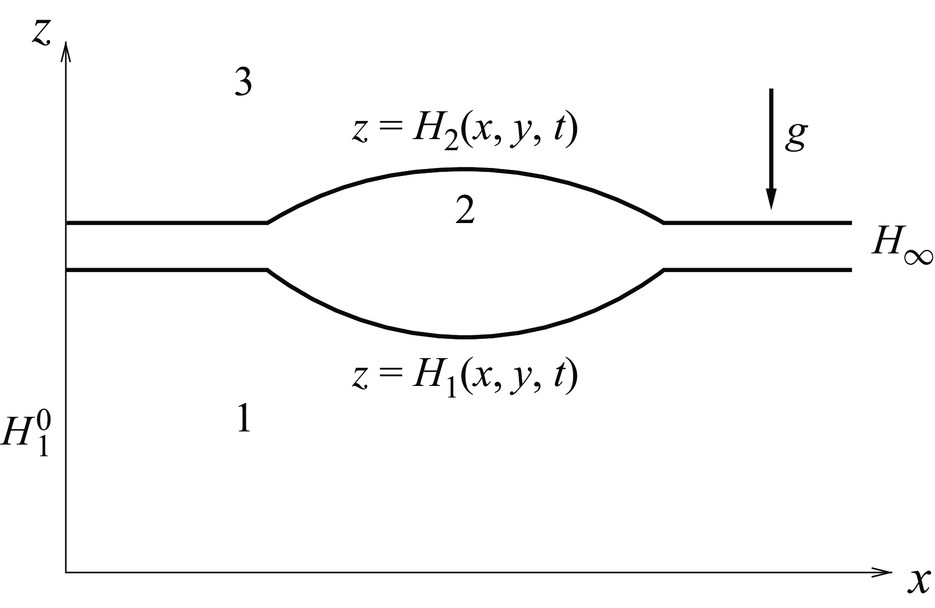
We consider a droplet of liquid 2 that floats on a layer of liquid 1. The droplet is in contact with the gas phase 3 (see figure 1). We do not consider any processes in fluid 3: the viscous stresses are neglected at the liquid/gas interface, and the heat transfer is described using the heat exchange coefficient $q$ . The $m$ th fluid has density $\rho _m$ , dynamic viscosity $\eta _m$ , and thermal conductivity $\kappa _m$ , $m=1, 2$ .

Figure 1.

Geometric configuration of the region and coordinate axes.

The temperature of the solid substrate is $T_s+{\tilde A}x$ , and the temperature of the gas near the interface is $T_g+{\tilde A}x$ . It is assumed that the interfacial tension coefficients on the lower and upper surfaces of the droplet are the linear functions of temperature $T$ : $\sigma _1=\sigma _1^0-\alpha _1 T$ , $\sigma _2=\sigma _2^0-\alpha _2 T$ , where $\alpha _1$ and $\alpha _2$ are constants. For the description of a floating droplet, we use the precursor model: the interface between fluids 1 and 3 outside the droplet is replaced by an ultra-thin precursor layer of fluid 2 (see figure 1). Far from the droplet, the equilibrium thickness of layer 1 is $H_1^0$ , and the thickness of the precursor film is $H_{\infty }$ . The deformable interfaces are described by equations $z=H_1(x,y,t)$ and $z=H_2(x,y,t)$ . The gravity acceleration is $g$ . We assume that the characteristic horizontal scale of the interface deformations is large compared to the characteristic vertical size of the droplet and the liquid substrate. In this case, the nonlinear models governing three-dimensional flows with deformable interfaces can be drastically simplified by the use of the lubrication approximation (see Pototsky et al. Reference Pototsky, Bestehorn, Merkt and Thiele2005; Nepomnyashchy & Simanovskii Reference Nepomnyashchy and Simanovskii2007). In the framework of the longwave approach, the shapes of the interfaces $z=H_1$ and $z=H_2$ depend on the scaled horizontal coordinates $X=\epsilon x$ and $Y=\epsilon y$ , $\epsilon \ll 1$ , rather than on $x$ and $y$ . Also, it is assumed that they depend on the scaled time variable $\tau =\epsilon ^2 t$ . There are several conditions for the applicability of that approach. First, the surface tension has to be strong, so that any shortwave deformation of the interfaces is suppressed. The analysis (see Oron, Davis & Bankoff Reference Oron, Davis and Bankoff1997) shows that the ratio of the characteristic thickness of the system in the vertical direction to the characteristic scale of the interfacial deformations in the horizontal direction is $O(\epsilon )$ , $\epsilon \ll 1$ , if the surface tension is $O(\epsilon ^{-1/2})$ . Also, the droplet has to be slender due to a small negative spreading coefficient or because of the action of the gravity. In that case, the velocity, pressure and temperature fields are enslaved to the interfacial deformations (see Pototsky et al. Reference Pototsky, Bestehorn, Merkt and Thiele2005). That circumstance allows us to reduce the difficult nonlinear problem to a closed system of evolution equations for variables that describe the shapes of interfaces.

The non-dimensional system of equations looks as follows (lowercase letters correspond to non-dimensional quantities):

(2.1) \begin{align} h_{1\tau }+\boldsymbol{\nabla }\boldsymbol{\cdot }\boldsymbol {q}_1=0,\quad h_{2\tau }+\boldsymbol{\nabla }\boldsymbol{\cdot }\boldsymbol {q}_2=0, \\[-28pt] \nonumber \end{align}

(2.2) \begin{align} \boldsymbol {q}_1=f_{11} \boldsymbol{\nabla } \kern-1pt \bar {p}_1+f_{12} \boldsymbol{\nabla } \kern-1pt \bar {p}_2+\boldsymbol {q}_1^{T},\quad\boldsymbol {q}_2=f_{21} \boldsymbol{\nabla } \kern-1pt \bar {p}_1+f_{22} \boldsymbol{\nabla } \kern-1pt \bar {p}_2+\boldsymbol {q}_2^{T}, \\[-28pt] \nonumber \end{align}

(2.3) \begin{align} f_{11}=-\frac {1}{3}h_1^3,\quad f_{12}=-\frac {1}{2}h_1^2(h_2-h_1), \\[-28pt] \nonumber \end{align}

(2.4) \begin{align} f_{21}=\frac {1}{6}h_1^3-\frac {1}{2}h_1^2h_2,\quad f_{22}= (h_2-h_1)\left [h_1^2\left (\frac {1}{2}-\frac {\eta }{3}\right ) +h_1h_2\left (-1+\frac {2\eta }{3}\right )-\frac {\eta }{3}h_2^2\right ]\!, \\[-28pt] \nonumber \end{align}

(2.5) \begin{align} \bar {p}_1=-{\nabla} ^2h_1-\sigma {\nabla} ^2h_2+{\textit{Bo}} h_1+{\textit{Bo}} \rho (h_2-h_1)+\pi _1(h_1,h_2), \\[-31pt] \nonumber \end{align}

(2.6) \begin{align} \bar {p}_2=-\sigma {\nabla} ^2h_2+{\textit{Bo}}\rho h_2+\pi _2(h_1,h_2), \\[-31pt] \nonumber \end{align}

(2.7) \begin{align} \boldsymbol {q}_1^T=\frac {{M}_{\bot }}{2}h_1^2\,\boldsymbol{\nabla }[d(\textit{Bih}_1-\alpha \kappa )]-\frac {M_{\|}}{2}(1+\alpha )h_1^2\boldsymbol {e}_x, \\[-31pt] \nonumber \end{align}

(2.8) \begin{align} \boldsymbol {q}_2^T & = \frac {{M}_{\bot }}{2} \big\{-h_2^2\,\boldsymbol{\nabla }(d\eta \alpha \kappa )+ (2h_2-h_1)h_1\,\boldsymbol{\nabla }\{d[Bi h_1-\alpha \kappa (1-\eta )]\} \big\}, \nonumber \\& \quad -\frac {M_{\|}}{2}\big[\eta \alpha (h_2-h_1)^2+(1+\alpha )h_1(2h_2-h_1)\big]\boldsymbol {e}_x,\\[-31pt] \nonumber \end{align}

(2.9) \begin{align} d=[\kappa +Bi (1-\kappa )h_1+Bi \kappa h_2]^{-1}. \\[-2pt] \nonumber \end{align}

Let us note that the system of equations describing the dynamics in the longwave limit is invariant with respect to the scaling transformation

(2.10) \begin{align}& X\to cX,\quad\tau \to c^4\tau ,\quad p_{\!j}\to c^2 p_{\!j},\quad\boldsymbol {q}_{\!j}\to c^3\boldsymbol {q}_{\!j},\quad M_{\bot }\to c^2M_{\bot },\quad M_{\|}\to c^3M_{\|}, \end{align}

(2.11) \begin{align}&\qquad\qquad\qquad\qquad\qquad\qquad\qquad\quad {\textit{Bo}}\to c^2 {\textit{Bo}}, \end{align}

where $c$ is an arbitrary number (see Nepomnyashchy & Simanovskii Reference Nepomnyashchy and Simanovskii2012). This means that in the case of a layer that is infinite in the horizontal direction, all the results obtained for definite values of the parameters ( $M_{\bot }$ , $M_{\|}$ , $Bo$ ) can be applied for the other sets of parameters found according to (2.10). That scaling invariance is caused by the absence of a characteristic horizontal length scale in the case of an infinite layer. Therefore, the scales for variables $\tau$ and $p$ , as well as parameters $M_{\bot }$ , $M_{\|}$ and $Bo$ , contain an arbitrary parameter $L^{*}$ corresponding to the horizontal length scale.

We choose

(2.12) \begin{equation} \tau ^*=\frac {\eta _1(L^*)^4}{\sigma _1^0 \big(H_1^0 \big)^3} \end{equation}

as a time scale, and

(2.13) \begin{equation} p^*=\frac {\sigma _1^0H_1^0}{(L^*)^2} \end{equation}

as a pressure scale.

The non-dimensional parameters of the problem are

(2.14) \begin{align}& M_{\bot }=\frac {\alpha _1(T_s-T_g)}{\sigma _1^0}\left (\frac {L^*}{H_1^0}\right )^2, \end{align}

(2.15) \begin{align}& M_{\|}=\frac {\alpha _1AL^*}{\sigma _1^0}\left (\frac {L^*}{H_1^0}\right )^2 \end{align}

as the modified transverse and longitudinal Marangoni numbers, respectively. Also,

(2.16) \begin{equation} {\textit{Bi}}=\frac {qH_1^0}{\kappa _2} \end{equation}

is the Biot number, $\eta =\eta _1/\eta _2$ , $\kappa =\kappa _1/\kappa _2$ , $\sigma =\sigma _2^0/\sigma _1^0$ , $\alpha =\alpha _2/\alpha _1$ , $\rho =\rho _2/\rho _1$ , and

(2.17) \begin{equation} {\textit{Bo}}=\frac {g\rho _1(L^*)^2}{\sigma _1^0} \end{equation}

is the Bond number.

One can see that each flow rate $\boldsymbol {q}_1^{T}$ and $\boldsymbol {q}_2^{T}$ contains two contributions, one proportional to $M_{\|}$ , and the other to $M_{\bot }$ . The former contribution, which is caused by the imposed horizontal temperature gradient, is always directed opposite to vector $\boldsymbol {e}_x$ , i.e. towards the region with lower temperature and hence higher interfacial tensions. Note that the contribution of the horizontal temperature gradient into $\boldsymbol{\nabla }\boldsymbol{\cdot }\boldsymbol {q}_1$ can be written as $u_1h_{1x}$ , where

(2.18) \begin{equation} u_1=-M_{\|}(1+\alpha ) h_1. \end{equation}

Thus each point of the droplet’s bottom surface moves to the left with the velocity (2.18). The term with $M_{\|}$ in the expression for $\boldsymbol{\nabla }\boldsymbol{\cdot }\boldsymbol {q}_2$ is $u_2h_{2x}+w_2$ , where

(2.19) \begin{align}& u_2=-M_{\|}[\eta \alpha (h_2-h_1)+(1+\alpha )h_1], \end{align}

(2.20) \begin{align}& w_2=M_{\|}[\eta \alpha -(1+\alpha )](h_2-h_1)h_{1x}. \end{align}

Thus in addition to the motion to the left with velocity (2.19), a point on the top surface of the droplet moves upwards or downwards with velocity (2.20).

The second contribution, proportional to $M_{\bot }$ , is generated by non-uniformities of the interfacial temperature field, which are caused by the deformations of interfaces.

Because the thickness of liquid layer 1 is always macroscopic, we can neglect the contribution of $\pi _1$ . In layer 2, we apply the following expression for the disjoining pressure:

(2.21) \begin{equation} \pi _2=\frac {a}{(h_2-h_1)^3} \left [1-\left (\frac {h_{\infty }}{h_2-h_1}\right )^3\right ]\!, \end{equation}

where $a$ is the non-dimensional Hamaker constant, which is related to the dimensional Hamaker constant $A$ as

(2.22) \begin{equation} a=\frac {A(L^*)^2}{6\pi \sigma _1^0 \big(H_1^0 \big)^4}, \end{equation}

and $h_{\infty }=H_{\infty }/H_1^0$ .

3. Nonlinear simulations

The problem governed by (2.1)–(2.21) was solved numerically with some initial conditions. The evolution equations were discretised by central differences for spatial derivatives, and solved using an explicit scheme. We use a grid with a constant spatial step, the central differences for spatial derivatives, and the approximation of the first order for temporal derivatives. The explicit scheme is stable for the chosen values of the time step. Periodic boundary conditions have been applied on the boundaries of the computational region $L \times L$ . Computations have been performed in the region $L \times L= 240\times 240$ using the grid $120\times 120$ . For moderate values of $M_{\bot }$ and $M_{\|}$ , the fields $h_1$ and $h_2$ are rather smooth, thus the grid $120\times 120$ gives a good resolution of large-scale wave patterns. Some trial simulations on the grids $100\times 100$ and $160\times 160$ did not reveal any qualitative changes. More details on the numerical scheme and the validation of the results are presented in the Appendix.

As initial conditions, we use a droplet of liquid 2 with a Gaussian shape that was imposed on a flat layer of liquid 1:

(3.1) \begin{align} h_1(X,Y,0)=1,\quad h_2(X,Y,0)=h_-+h_+\exp \big\{-\big[(X-L/2)^2+(Y-L/2)^2\big]/R^2\big\}, \end{align}

where $h_{-}$ , $h_{+}$ corresponding to the initial shape of the droplet are constants, and $R$ is the radius of the droplet. In some other simulations, in order not to lose the information obtained on the previous time steps, we used as the initial condition a solution formerly obtained for another set of parameters. The computations have been performed for the system of fluorinert FC70 (liquid 1) and silicon oil 10 (liquid 2), which was used in microgravity experiments (see e.g. Géoris et al. Reference Géoris, Hennenberg, Lebon and Legros1999). The following set of liquid parameters has been applied: $\eta =3.04$ , $\kappa =0.522$ , $\alpha =2$ , $\rho =0.482$ , $\sigma =2.6$ , $h_-=1.02$ , $h_+=1$ , $R=20$ , $h_{\infty }=0.02$ and ${\textit{Bi}}=20$ (see Nepomnyashchy & Simanovskii Reference Nepomnyashchy and Simanovskii2007). The value of $a$ was chosen to be $0.1\times 10^{-5}$ . The primary analysis of the obtained nonlinear regimes has been performed using snapshots of the fields of $h_{\!j}(X,Y,\tau ),$ $j=1,2$ . The analysis has been supplemented by the investigation of the time dependence for the maximum values of the variables $h_{\!j},$

(3.2) \begin{equation} h_{ \textit{max},j}(\tau )=\max h_{j}(X,Y,\tau ), \end{equation}

and Fourier components

(3.3) \begin{align}& c_{m,n}(\tau )=\frac {2}{L^2}\int _0^{L}\int _0^{L}h_1(X,Y,\tau ) \cos \left [\frac {2\pi X}{L}(mX+nY)\right ]{\rm d}X\, {\rm d}Y, \end{align}

(3.4) \begin{align}& s_{m,n}(\tau )=\frac {2}{L^2}\int _0^{L}\int _0^{L}h_1(X,Y,\tau ) \sin \left [\frac {2\pi X}{L}(mX+nY)\right ]{\rm d}X\, {\rm d}Y, \end{align}

where $m,n$ are integer numbers.

We have used also quantities

(3.5) \begin{equation} r_{m,n}(\tau )=\sqrt {c_{m,n}^2(\tau )+s_{m,n}^2(\tau )}, \end{equation}

characterising the amplitudes of corresponding complex Fourier harmonics.

3.1. The case of a constant temperature gradient

First, let us describe the results of nonlinear simulations in the case of homogeneous heating. We take ${\textit{Bo}}=0$ . The simplest structure observed for sufficiently small values of $M_{\|}$ and $|M_{\bot }|$ is the droplet, moving from right to left as a whole (Nepomnyashchy & Simanovskii Reference Nepomnyashchy and Simanovskii2025):

(3.6) \begin{equation} h_{\!j}=h_{\!j}(X+c\tau ),\quad j=1,2,\ c\gt 0. \end{equation}

The snapshots of the fields of $h_2(X,Y,\tau )$ at different instants of time are shown in figure 2. In all figures showing the droplet, the horizontal axis is $X$ and the vertical axis is $Y$ . The shapes of interfaces corresponding to figure 2(b) are shown in figure 3.

Figure 2.

The fields of $h_2(X,Y,\tau )$ for $M_{\bot }=-0.1$ , $M_{\|}=0.0001$ , ${\textit{Bo}}=0$ , ${\textit{Bi}}=20$ , for (a) $\tau =780\,000$ , (b) $\tau =860\,000$ , (c) $\tau =930\,000$ , (d) $\tau =1\times10^6$ .

Figure 3.

The shapes of interfaces (a) $h_2(X,Y,\tau )$ and (b) $h_1(X,Y,\tau )$ for $M_{\bot }=-0.1$ , $M_{\|}=0.0001$ , ${\textit{Bo}}=0$ , ${\textit{Bi}}=20$ , $\tau =860\,000$ .

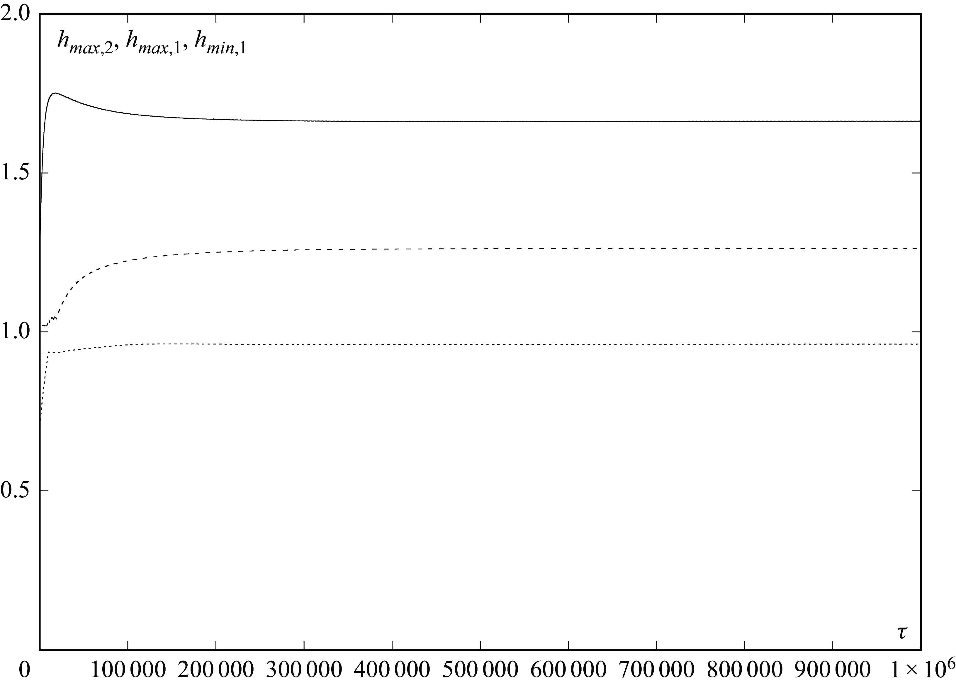
This type of motion has also been found in the presence of the gravity force (at $Bo \neq 0$ ). The temporal evolution of $h_{ \textit{max},j}$ , $j=1,2$ , and $h_{ \textit{min},1}$ leading to the formation of the steady droplet is shown in figure 4. The snapshots of $h_2(X,Y,\tau )$ for ${\textit{Bo}}=0.02$ ( $M_{\bot }=-0.1$ , $M_{\|}=0.0001$ ) are shown in figure 5. As in the previous case, the droplet moves from the right-hand side to the left-hand side. The height of the droplet is lower than that in the case at ${\textit{Bo}}=0$ (cf. for instance, figures 5(b) and 2(a)). The shapes of interfaces corresponding to figure 5(d) are presented in figure 6. At the larger values of the gravity force (we take ${\textit{Bo}}=0.1$ ), the interfaces of the droplet are essentially flattened. The droplet moves from right to left. The snapshots of $h_2(X,Y,\tau )$ for ${\textit{Bo}}=0.1$ ( $M_{\bot }=-0.1$ , $M_{\|}=0.0001$ ) are shown in figure 7, and the shape of the interface corresponding to figure 7(a) is shown in figure 8.

Figure 4.

The dependences of $h_{ \textit{max},2}(\tau )$ (solid line), $h_{ \textit{max},1}(\tau )$ (dashed line) and $h_{ \textit{min},1}(\tau )$ (dotted line) on time for $M_{\bot }=-0.1$ , $M_{\|}=0.0001$ , ${\textit{Bo}}=0.02$ , ${\textit{Bi}}=20$ .

Figure 5.

The fields of $h_2(X,Y,\tau )$ for $M_{\bot }=-0.1$ , $M_{\|}=0.0001$ , ${\textit{Bo}}=0.02$ , ${\textit{Bi}}=20$ , for (a) $\tau =630\,000$ , (b) $\tau =710\,000$ , (c) $\tau =790\,000$ , (d) $\tau =870\,000$ .

Figure 6.

The shapes of interfaces (a) $h_2(X,Y,\tau )$ and (b) $h_1(X,Y,\tau )$ for $M_{\bot }=-0.1$ , $M_{\|}=0.0001$ , ${\textit{Bo}}=0.02$ , ${\textit{Bi}}=20$ , $\tau =870\,000$ .

Figure 7.

Snapshots of the fields $h_2(X,Y,\tau )$ for $M_{\bot }=-0.1$ , $M_{\|}=0.0001$ , ${\textit{Bo}}=0.1$ , ${\textit{Bi}}=20$ , for (a) $\tau =700\,000$ , (b) $\tau =780\,000$ , (c) $\tau =860\,000$ , (d) $\tau =940\,000$ .

Figure 8.

The shape of the interface $h_2(X,Y,\tau )$ for $M_{\bot }=-0.1$ , $M_{\|}=0.0001$ , ${\textit{Bo}}=0.1$ , ${\textit{Bi}}=20$ , $\tau =700\,000$ .

Now let us take as the initial conditions the regime presented in figure 6, and consider its evolution at sufficiently large values of $|M_{\bot }|$ and $M_{\|}$ . The snapshots of the fields of $h_2(X,Y,\tau )$ for $M_{\bot }=-1$ and $M_{\|}=0.001$ at different instants of time are shown in figure 9. Though the droplet is of a rather complicated (‘swallow-like’) shape, it moves from the right–hand side to the left–hand side as a whole:

(3.7) \begin{equation} h_{\!j}=h_{\!j}(X+c\tau ),\quad j=1,2,\ c\gt 0. \end{equation}

Figure 9.

Snapshots of the fields $h_2(X,Y,\tau )$ for $M_{\bot }=-1$ , $M_{\|}=0.001$ , ${\textit{Bo}}=0.02$ , ${\textit{Bi}}=20$ , for (a) $\tau =2.35\times 10^6$ , (b) $\tau =2.42\times 10^6$ , (c) $\tau =2.49\times 10^6$ , (d) $\tau =2.57\times 10^6$ .

The shapes of the interfaces corresponding to figure 9(c) are presented in figure 10.

Figure 10.

The shapes of interfaces (a) $h_2(X,Y,\tau )$ and (b) $h_1(X,Y,\tau )$ for $M_{\bot }=-1$ , $M_{\|}=0.001$ , ${\textit{Bo}}=0.02$ , ${\textit{Bi}}=20$ , $\tau =2.49\times 10^6$ .

3.2. The case of a modulated temperature gradient

Below, we discuss the nonlinear regimes observed in the case of a spatial modulation of the local Marangoni number,

(3.8) \begin{equation} M_{\bot }(X)=\bar {M}_{\bot }\left (1+\delta _X\sin \frac { 2\pi X}{L}\right )=\bar {M}_{\bot }-\varDelta _X\sin \frac {2\pi X}{L}, \end{equation}

where $\bar {M}_{\bot }\lt 0$ , $\delta _X\gt 0$ , $\varDelta _X=|\bar {M}_{\bot }|\,\delta _X$ .

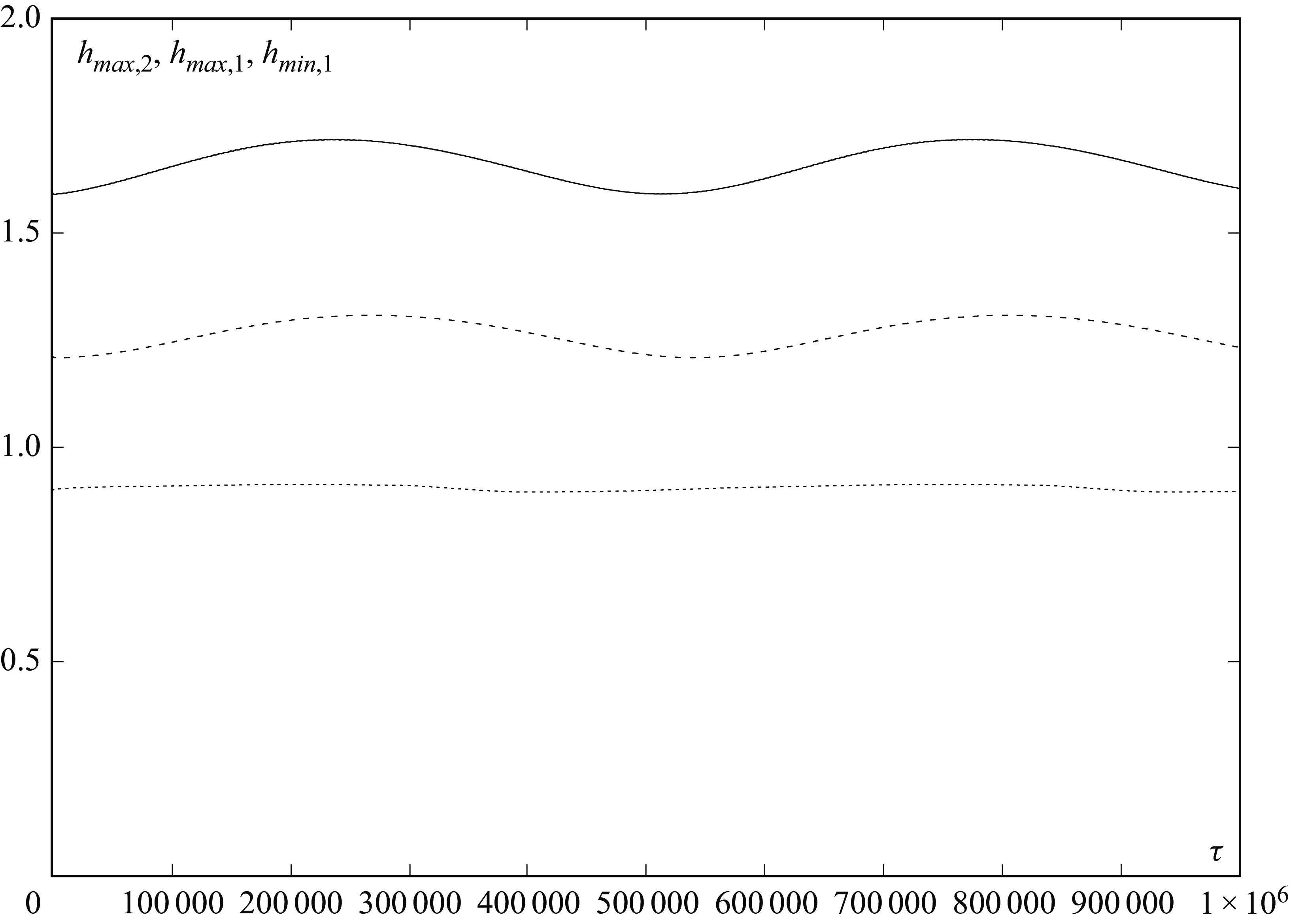
Let us take the droplet presented in figure 5 ( $M_{\bot }=-0.1$ , $M_{\|}=0.0001$ , $\varDelta _X=0$ ) as the initial condition, and consider its evolution under the action of modulation of the transverse Marangoni number ( $\bar {M}_{\bot }=-0.1$ , $\varDelta _X=0.025$ ). The temporal evolution of $h_{ \textit{max},2}$ , $h_{ \textit{max},1}$ and $h_{ \textit{min},1}$ is shown in figure 11. One can see that $h_{ \textit{max},j}$ , $j=1, 2$ , and $h_{ \textit{min},1}$ change in time (cf. figures 4 and 11). The two-dimensional snapshots of the fields $h_2(X,Y,\tau )$ at different instants of time are shown in figure 12. The droplet moves slowly from right to left passing the spatial modulation period $L$ during the time interval $T=556\,000$ . Correspondingly, the shape of the droplet oscillates with the period $T$ . The shapes of the interfaces corresponding to figure 12(a) are presented in figure 13.

Figure 11.

The temporal evolution of $h_{ \textit{max},2}(\tau )$ (solid line), $h_{ \textit{max},1}(\tau )$ (dashed line) and $h_{ \textit{min},1}(\tau )$ (dotted line) for $\bar {M}_{\bot }=-0.1$ , ${M_{\|}}=0.0001$ , $\varDelta _X=0.025$ , ${\textit{Bo}}=0.02$ , ${\textit{Bi}}=20$ .

Figure 12.

The fields of $h_2(X,Y,\tau )$ for $\bar {M}_{\bot }=-0.1$ , ${M_{\|}}=0.0001$ , $\varDelta _X=0.025$ , ${\textit{Bo}}=0.02$ , ${\textit{Bi}}=20$ , for (a) $\tau =330\,000$ , (b) $\tau =468\,500$ , (c) $\tau =607\,000$ , (d) $\tau =744\,500$ .

Figure 13.

The shapes of interfaces (a) $h_2(X,Y,\tau )$ and (b) $h_1(X,Y,\tau )$ for $\bar {M}_{\bot }=-0.1$ , ${M_{\|}}=0.0001$ , $\varDelta _X=0.025$ , ${\textit{Bo}}=0.02$ , ${\textit{Bi}}=20$ , $\tau =330\,000$ .

With an increase of the transverse Marangoni number (we take $\bar {M}_{\bot }=-1$ ), the droplet moving from right to left is significantly deformed. The two-dimensional snapshots of the fields $h_2(X,Y,\tau )$ at different instants of time are shown in figure 14. The shapes of the interfaces corresponding to figure 14(a) are presented in figure 15. One can see that the droplet becomes higher than that in the case $\bar {M}_{\bot }=-0.1$ (cf. figures 13 and 15).

Figure 14.

The fields of $h_2(X,Y,\tau )$ for $\bar {M}_{\bot }=-1$ , ${M_{\|}}=0.0001$ , $\varDelta _X=0.025$ , ${\textit{Bo}}=0.02$ , ${\textit{Bi}}=20$ , for (a) $\tau =150\,000$ , (b) $\tau =200\,000$ , (c) $\tau =235\,000$ , (d) $\tau =285\,000$ .

Figure 15.

The shapes of interfaces (a) $h_2(X,Y,\tau )$ and (b) $h_1(X,Y,\tau )$ for $\bar {M}_{\bot }=-1$ , ${M_{\|}}=0.0001$ , $\varDelta _X=0.025$ , ${\textit{Bo}}=0.02$ , ${\textit{Bi}}=20$ , $\tau =150\,000$ .

Let us take as the initial conditions the droplet presented in figures 9(c) and 10, and consider its evolution under the action of the modulation of the transverse temperature gradient ( $\varDelta _X=0.025$ ). The temporal evolution of $h_{ \textit{max},2}$ , $h_{ \textit{max},1}$ and $h_{ \textit{min},1}$ is shown in figure 16. One can see that the fields $h_{ \textit{max},j}$ , $j=1, 2$ , and $h_{ \textit{min},1}$ change in time in a periodic way. The phase trajectory in the plane $(r_{10}, r_{01})$ confirms the periodic character of oscillations (see figure 17). The two-dimensional snapshots of the fields $h_2(X,Y,\tau )$ at different instants of time are shown in figure 18, and three-dimensional shapes of interfaces corresponding to figure 18(e) are presented in figure 19. The droplet moves from right to left changing the shape during the oscillatory process. During the period of oscillations $T=41\,850$ , the droplet passes the distance $L$ equal to the spatial period of the temperature modulation.

Figure 16.

The temporal evolution of $h_{ \textit{max},2}(\tau )$ (solid line), $h_{ \textit{max},1}(\tau )$ (dashed line) and $h_{ \textit{min},1}(\tau )$ (dotted line) for $\bar {M}_{\bot }=-1$ , ${M_{\|}}=0.001$ , $\varDelta _X=0.025$ , ${\textit{Bo}}=0.02$ , ${\textit{Bi}}=20$ .

Figure 17.

The phase trajectory in the plane $(r_{10}, r_{01})$ for $\bar {M}_{\bot }=-1$ , ${M_{\|}}=0.001$ , $\varDelta _X=0.025$ , ${\textit{Bo}}=0.02$ , ${\textit{Bi}}=20$ .

Figure 18.

The fields of $h_2(X,Y,\tau )$ for $\bar {M}_{\bot }=-1$ , ${M_{\|}}=0.001$ , $\varDelta _X=0.025$ , ${\textit{Bo}}=0.02$ , ${\textit{Bi}}=20$ , for (a) $\tau =300\,000$ , (b) $\tau =308\,500$ , (c) $\tau =315\,000$ , (d) $\tau =323\,500$ , (e) $\tau =331\,200$ , (f) $336\,000$ .

Figure 19.

The shapes of interfaces (a) $h_2(X,Y,\tau )$ and (b) $h_1(X,Y,\tau )$ for $\bar {M}_{\bot }=-1$ , ${M_{\|}}=0.001$ , $\varDelta _X=0.025$ , ${\textit{Bo}}=0.02$ , ${\textit{Bi}}=20$ , $\tau =331\,200$ .

Let us now increase the transverse temperature modulation – we take $\varDelta _X=0.05$ ( $\bar {M}_{\bot }=-1$ , $M_{\|}=0.001$ ). Since one of the frequencies is due to the instability and the other is due to the passing the temperature modulation period $L$ by the droplet, we observe quasi-periodic oscillations. The temporal evolution of $h_{ \textit{max},2}$ , $h_{ \textit{max},1}$ and $h_{ \textit{min},1}$ is shown in figure 20. Different maxima of $h_{ \textit{max},j}(\tau )$ , $j=1,2$ , correspond to different spatial points. Let us note that because the different maxima are in the points with different values of $\bar {M}_{\bot }$ , there is no reason for them to be equal. The phase trajectory in the plane $(r_{10}, r_{01})$ confirms the quasi-periodic character of oscillations (see figure 21).

Figure 20.

The temporal evolution of $h_{ \textit{max},2}(\tau )$ (solid line), $h_{ \textit{max},1}(\tau )$ (dashed line) and $h_{ \textit{min},1}(\tau )$ (dotted line) for $\bar {M}_{\bot }=-1$ , ${M_{\|}}=0.001$ , $\varDelta _X=0.05$ , ${\textit{Bo}}=0.02$ , ${\textit{Bi}}=20$ .

Figure 21.

The phase trajectory in the plane $(r_{10}, r_{01})$ for $\bar {M}_{\bot }=-1$ , ${M_{\|}}=0.001$ , $\varDelta _X=0.05$ , ${\textit{Bo}}=0.02$ , ${\textit{Bi}}=20$ .

The two-dimensional snapshots of the fields $h_2(X,Y,\tau )$ at different instants of time are shown in figure 22. One can see a visible change of the droplet shape between figures 22(a) and 22(c). The division of the ‘main’ droplet and the creation of the satellites are presented in figures 22(d) and 22(e). The ‘main’ droplet as well as the appeared satellites move from the right–hand side to the left–hand side, changing shape during an oscillatory process. The merging of the satellites with the ‘main’ droplet is shown in figure 22(f). The separation and the recombination of the ‘main’ droplet with its satellites could be the origin of oscillations. The shapes of the interfaces corresponding to figure 22(e) are presented in figure 23. Note that locations of the deformations on both interfaces are correlated.

Figure 22.

The fields of $h_2(X,Y,\tau )$ for $\bar {M}_{\bot }=-1$ , ${M_{\|}}=0.001$ , $\varDelta _X=0.05$ , ${\textit{Bo}}=0.02$ , ${\textit{Bi}}=20$ , for (a) $\tau =100\,000$ , (b) $\tau =104\,000$ , (c) $\tau =112\,500$ , (d) $\tau =125\,000$ , (e) $\tau =129\,000$ , (f) $\tau =135\,700$ .

Figure 23.

The shapes of interfaces (a) $h_2(X,Y,\tau )$ and (b) $h_1(X,Y,\tau )$ for $\bar {M}_{\bot }=-1$ , ${M_{\|}}=0.001$ , $\varDelta _X=0.05$ , ${\textit{Bo}}=0.02$ , ${\textit{Bi}}=20$ , $\tau =129\,000$ .

4. The action of gravity on the moving droplets

Let us consider the action of the gravity force on the droplets dynamics in the presence of the spatial modulation of the transverse Marangoni number. We use as initial conditions the droplet shown in figure 12 ( ${\textit{Bo}}=0.02$ ), and increase the gravity force (we take ${\textit{Bo}}=0.1$ ). The two-dimensional snapshots of the fields $h_2(X,Y,\tau )$ at different instants of time are presented in figure 24. The droplet moving from right to left is significantly flattened (cf. for instance, figures 12(a) and 24(c)). The three-dimensional shape of the interface $h_2(X,Y,\tau )$ corresponding to figure 24(a) is shown in figure 25.

Figure 24.

The fields of $h_2(X,Y,\tau )$ for $\bar {M}_{\bot }=-1$ , ${M_{\|}}=0.0001$ , $\varDelta _X=0.025$ , ${\textit{Bo}}=0.1$ , ${\textit{Bi}}=20$ , for (a) $\tau =100\,000$ , (b) $\tau =180\,000$ , (c) $\tau =260\,000$ , (d) $\tau =340\,000$ .

Figure 25.

The shape of the interface $h_2(X,Y,\tau )$ for $\bar {M}_{\bot }=-1$ , ${M_{\|}}=0.0001$ , $\varDelta _X=0.025$ , ${\textit{Bo}}=0.1$ , ${\textit{Bi}}=20$ , $\tau =100\,000$ .

5. The influence of the period of spatial modulation and the initial droplet radius on the droplet shape

We have also analysed the influence of the period of spatial modulation $L$ , and the initial droplet radius $R$ , on the shape and the motion of the droplet.

The influence of the enhancement of $L$ is twofold. First, according to (3.8), the spatial gradient of $M_{\bot }(X)$ is diminished. Second, the distance between the droplets that form a periodic sequence is enhanced, hence the interaction between them is weakened. We made simulations in the computational region $2L \times 2L$ , taking the grid $240 \times 240$ . We got periodic oscillations of a single droplet again. The two-dimensional snapshots of the fields $h_2(X,Y,\tau )$ at different instants of time are shown in figure 26. One can see the creation of satellites in figures 26(c) and 26(d). The ‘main’ droplet as well as the appeared satellites move from right to left, changing shape during an oscillatory process.

Figure 26.

The fields of $h_2(X,Y,\tau )$ for $\bar {M}_{\bot }=-1$ , ${M_{\|}}=0.001$ , $\varDelta _X=0.025$ , $R=20$ , ${\textit{Bo}}=0.02$ , ${\textit{Bi}}=20$ , for (a) $\tau =530\,000$ , (b) $\tau =552\,500$ , (c) $\tau =560\,000$ , (d) $\tau =578\,500$ , with $L=480$ and grid $240\times 240$ .

Comparison of figures 18 and 26 shows that the swallow-tail shape of the droplet persists. The enhancement of the droplet size (see figure 27) restores the interaction of the droplets but does not qualitatively change their shape.

Figure 27.

The fields of $h_2(X,Y,\tau )$ for $\bar {M}_{\bot }=-1$ , ${M_{\|}}=0.001$ , $\Delta _X=0.025$ , $R=40$ , ${\textit{Bo}}=0.02$ , ${\textit{Bi}}=20$ , for (a) $\tau =410\,000$ , (b) $\tau =418\,500$ , (c) $\tau =430\,000$ , (d) $\tau =438\,500$ , with $L=480$ and grid $240\times 240$ .