

1. Introduction
Flows in the atmosphere and the ocean are composed of fast evolving dispersive inertia-gravity waves and slowly evolving geostrophically balanced vortical flows. The rotating shallow water equations (RSWE) are one of the simplest models that can capture fast waves, the slow vortical field and their nonlinear interactions. Consequently, RSWE has been a workhorse for a broad variety of investigations on turbulent dynamics of waves and balanced flow in connection to the atmosphere and the ocean (Salmon Reference Salmon1978; Vallis Reference Vallis2006; Zeitlin Reference Zeitlin2018).
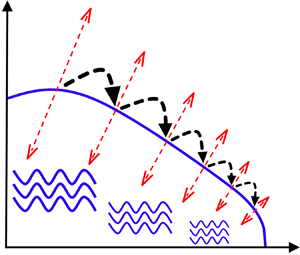
Although external forcing mechanisms excite large-scale inertia-gravity waves in the atmosphere and the ocean, these waves transfer their energy downscale via a forward cascade, eventually dissipating their energy at small viscous scales. Understanding the details of this energy transfer pathway is crucial for developing better parametrizations for waves’ downscale fluxes and small-scale mixing in large climate-scale models. As a result, theoretical and numerical pursuits have been undertaken in the past to explore the turbulent downscale transfer of waves in a wide range of geophysical flow models. In this paper we will focus on some of the features of the turbulent cascade of inertia-gravity waves in RSWE, specifically in the weakly nonlinear regime.
The dynamics in the weakly nonlinear regime is generated by the nonlinear interaction of linear modes and is a result of small amplitude waves or the smallness of flow velocity compared with gravity wave speeds and smallness of height fluctuations with respect to the mean height of the flow. In this regime, asymptotic analysis and resonant wave interaction theory can be used to predict different kinds of interactions that can lead to energy exchange between waves; see for example resonant wave interaction theory and its applications to different fluid flow models in Phillips (Reference Phillips1981) and Craik (Reference Craik1985).
The dispersion relationship of inertia-gravity waves in RSWE does not allow triadic resonant wave–wave–wave (WWW) interactions (Babin, Mahalov & Nicolaenko Reference Babin, Mahalov and Nicolaenko1997; Majda Reference Majda2002). As a result, the only kind of triadic interactions waves participate in are those involving geostrophic or vortical modes. Vortical modes can scatter wave energy between wave modes that have the same wavenumber magnitude  $k$ (see discussions in Majda (Reference Majda2002) and Ward & Dewar (Reference Ward and Dewar2010)). This means that vortical scattering of waves with wavenumber magnitude
 $k$ can only rearrange wave energy within rings in spectral space satisfying
 $k = \text {const.}$, contrary to the case in three dimensions where vortical modes can facilitate the downscale transfer of wave energy from large inviscid scales to small dissipative scales (Lelong & Riley Reference Lelong and Riley1991; Bartello Reference Bartello1995; Thomas & Daniel Reference Thomas and Daniel2020). Therefore, asymptotic calculations using resonant wave interaction theory rules out the possibility of an efficient downscale transfer of wave energy in RSWE via triadic resonances. Resonant WWW triads do not exist while resonant WVW triadic interactions retain wave energy within the same scales, i.e.
 $k = \text {const.}$ rings.
Despite weakly nonlinear asymptotic calculations leading to the above-mentioned conclusions, RSWE are primarily the shallow water equations with the addition of the Coriolis term. Furthermore, the non-rotating shallow water equations are the exact equations that govern the dynamics of a compressible gas with  $-2$ as the ratio of specific heats (Vallis Reference Vallis2006). Therefore, similar to the case in compressible flows, an arbitrary wave field evolving based on the non-rotating shallow water equations would steepen and form shock waves. An ensemble of waves would generate a wave spectrum that is close to
 $k^{-2}$, a spectrum that is expected for a flow consisting of a distribution of discontinuities such as shocks (Kuznetsov Reference Kuznetsov2004; Falkovich & Kritsuk Reference Falkovich and Kritsuk2017). Recently, Augier, Mohanan & Lindborg (Reference Augier, Mohanan and Lindborg2019) simulated the non-rotating shallow water equations excluding the vorticity field and demonstrated an unambiguous
 $k^{-2}$ spectrum associated with gravity waves forming shocks.
Above-mentioned comparisons bring out the disparity between the asymptotic results on waves in RSWE and results expected from waves in RSWE based on compressible flow considerations. The asymptotic results on waves in RSWE are based on calculations that completely discard the possibility of shock formation. Since RSWE is basically a modification of the shallow water equations – a model in which waves always form shocks – one might naturally anticipate shocks in RSWE. However, the issue is non-trivial since rotation makes waves in RSWE dispersive, a feature that might affect shock formation. How severe the influence of rotation is on shock formation is unclear at this point. Additionally, if waves in RSWE form shocks, that raises new questions regarding the role of the vortical mode on wave dynamics. As mentioned earlier, in the absence of shocks, resonant wave interaction theory predicts that inertia-gravity waves would be scattered by vortices to waves of different wavenumbers with the same wavenumber magnitude. In contrast, it remains unclear how vortices would affect waves that could form shocks. Can a vortical field enhance or diminish the rate at which waves form into shocks? Exploring these questions, regarding the effects of rotation and the vortical mode on the turbulent cascade of inertia-gravity waves in RSWE is the focus of this work. Although multiple previous studies have explored RSWE using numerical simulations, it is noteworthy that only a handful of them have reported shock formation.
Farge & Sadourny (Reference Farge and Sadourny1989) was one of the earliest studies that attempted to explore the dynamics of RSWE using numerical simulations, although there is no indication of shock formation in their study (see their divergence fields given in their figure 3 and related explanation), which is not surprising since their resolution was  $128^2$, resulting in the largest wavenumber being
 $k_{max}=64$. With such a low resolution and their high wavenumbers
 $k \sim 50$ being affected by viscous dissipation, there is little range of scales left for capturing shocks. Polvani et al. (Reference Polvani, McWilliams, Spall and Ford1994) and Yuan & Hamilton (Reference Yuan and Hamilton1994) are numerical investigations of RSWE that followed Farge & Sadourny (Reference Farge and Sadourny1989). Polvani et al. (Reference Polvani, McWilliams, Spall and Ford1994) used freely evolving simulations initialized with geostrophic balanced flow alone, resulting in the generation of weak inertia-gravity waves with time. Polvani et al. report observations of weak shocks in some of their experiments (see their figure 7 and related discussion), although these waves played no role in the flow dynamics due to their insignificant strength. Yuan & Hamilton used a forced-dissipative set up to study RSWE and forced only the geostrophic balanced flow. Although weak inertia-gravity waves were seen to be excited at scales close to dissipative scales in their study, Yuan & Hamilton make no observations of shock formation. Following these, Lahaye & Zeitlin (Reference Lahaye and Zeitlin2012) re-examined flow dynamics of RSWE using numerical simulations. In one of their experiments initialized with inertia-gravity waves alone, they found the physical fields to be rich with shocks (see their figure 6 and related discussion). However, contrary to the
 $k^{-2}$ spectrum expected for a field rich with discontinuities like shocks, Lahaye & Zeitlin report a steep wave energy spectrum, close to
 $k^{-6}$. Such a steep wave energy spectrum is counterintuitive for a field that is rich with shocks, and raises more questions regarding waves and shocks in RSWE.
The discussion so far brings out the lack of clarity regarding the turbulent dynamics and forward cascade of inertia-gravity waves in RSWE. For an arbitrary flow in RSWE composed of waves and balanced flow, it is unclear if waves would remain as linear dispersive waves or if they would steepen and form shocks as seen in compressible flows. At least two reasons could be attributed towards such a gap in our understanding of turbulent inertia-gravity wave dynamics in RSWE. First, the earlier works, such as Farge & Sadourny (Reference Farge and Sadourny1989), that were performed more than three decades ago were constrained by the numerical resolution affordable at that time. The limited numerical resolutions made it challenging to capture small-scale waves and steep shock-like features. Second, although flows in the atmosphere and the ocean consists of fast waves and slow geostrophic flow, advances up until two decades or so ago were directed at improving our understanding of the large-scale balanced vortical flow, inspiring the studies of the nature discussed in Yuan & Hamilton (Reference Yuan and Hamilton1994) and Polvani et al. (Reference Polvani, McWilliams, Spall and Ford1994). In contrast, especially in the oceanographic context, the past two decades of observational and large-scale ocean model outputs have revealed that dispersive waves can be highly energetic in several oceanic regions of the world, with the wave energy levels often dominating over the balanced flow energy (see discussions in Thomas (Reference Thomas2023)). Consequently, it is imperative to develop a deeper understanding of dispersive wave turbulence in RSWE, this being one of the simplest reduced models used for geophysical fluid dynamics research. In our former work we investigated features associated with the inverse flux of inertia-gravity waves in RSWE in the weakly nonlinear regime (Thomas & Ding Reference Thomas and Ding2023). In contrast, in this work we will explore the features associated with the forward flux of inertia-gravity waves in RSWE in the weakly nonlinear regime using numerical integration of the governing equations.
The plan for the paper is as follows: we describe the model and its features in § 2; detail our results in §§ 3 and 4; and summarize our findings in § 5.
2. The model and its features
The RSWE on the  $f$-plane are
 $$\begin{gather} \frac{\partial{\boldsymbol{v}}}{\partial{t}} + \boldsymbol{f} \times \boldsymbol{v} + g \boldsymbol{\nabla} h + \boldsymbol{v} \boldsymbol{\cdot} \boldsymbol{\nabla} \boldsymbol{v} = 0, \end{gather}$$
 $$\begin{gather}\frac{\partial{h}}{\partial{t}} + H \boldsymbol{\nabla} \boldsymbol{\cdot} \boldsymbol{v} + \boldsymbol{\nabla} \boldsymbol{\cdot} (h \boldsymbol{v}) = 0, \end{gather}$$
where  $\boldsymbol {v} =(u, v)$ is the horizontal velocity,
 $h$ is the height field fluctuation with respect to the mean height
 $H$,
 $\boldsymbol {f} = f \boldsymbol {\hat {z}}$ with
 $f$ being the constant rotation rate and
 $\boldsymbol {\hat {z}}$ being the unit vector in the
 $z$-direction and
 $\boldsymbol {\nabla } = ( \partial /\partial x, \partial /\partial y )$ is the gradient operator. We scale the above equations as
 \begin{equation} \boldsymbol{x} \rightarrow L \boldsymbol{x}, \quad t \rightarrow \frac{L}{c_0} t, \quad f \rightarrow \frac{c_0}{L} f, \quad \boldsymbol{v} \rightarrow \left( \epsilon c_0 \right) \boldsymbol{v}, \quad h \rightarrow \left( \epsilon H \right) h. \end{equation}
In the above non-dimensionalization, the  $x$ and
 $y$ coordinates were scaled by a length scale
 $L$, which may be thought of as the length of the domain. Here
 $c_0 = \sqrt {g H}$ represents the phase speed of non-rotating gravity waves and we used the time scale
 $L/c_0$ to scale time. The velocity was scaled by
 $\epsilon c_0$ while the height field fluctuations with respect to the mean were scaled by
 $\epsilon H$. Notice that
 $\epsilon = U/c_0$, where
 $U$ may be thought of as an estimate for the dimensional flow velocity. Therefore,
 $\epsilon$ is the Froude number, providing us an estimate of how the flow velocity scales with linear non-rotating gravity wave speed. Throughout this paper we will be based in the weakly nonlinear regime characterized by
 $\epsilon \ll 1$. Consequently, from the above scaling we have
 $h \ll H$ (in dimensional form), which means that the fluctuations are small compared with the mean height. Applying the scaling (2.2a–e) to (2.1) gives us the following non-dimensional equations:
 $$\begin{gather} \frac{\partial{\boldsymbol{v}}}{\partial{t}} + \boldsymbol{f} \times \boldsymbol{v} + \boldsymbol{\nabla} h + \epsilon \boldsymbol{v} \boldsymbol{\cdot} \boldsymbol{\nabla} \boldsymbol{v} = 0, \end{gather}$$
 $$\begin{gather}\frac{\partial{h}}{\partial{t}} + \boldsymbol{\nabla} \boldsymbol{\cdot} \boldsymbol{v} + \epsilon \boldsymbol{\nabla} \boldsymbol{\cdot}(h \boldsymbol{v}) = 0. \end{gather}$$
2.1. The wave–vortex decomposition and the potential vorticity field
The solutions of the linear equations obtained by setting  $\epsilon =0$ in (2.3) consist of inertia-gravity waves and a divergence-free vortical mode that is in geostrophic balance. The equations governing these two fields, denoted with subscripts ‘W’ and ‘V’ for waves and vortical mode, are
 $$\begin{gather} \frac{\partial{ {{ \boldsymbol{v}}_{\scriptscriptstyle{W}}} }}{\partial{t}} + \boldsymbol{f} \times {{ \boldsymbol{v}}_{\scriptscriptstyle{W}}} + \boldsymbol{\nabla} {{h}_{\scriptscriptstyle{W}}} = 0 , \end{gather}$$
 $$\begin{gather}\frac{\partial{{{h}_{\scriptscriptstyle{W}}}}}{\partial{t}} + \boldsymbol{\nabla} \boldsymbol{\cdot} {{ \boldsymbol{v}}_{\scriptscriptstyle{W}}}=0, \end{gather}$$
 $$\begin{gather} \boldsymbol{f} \times {{ \boldsymbol{v}}_{\scriptscriptstyle{V}}} + \boldsymbol{\nabla} {{h}_{\scriptscriptstyle{V}}} = 0, \end{gather}$$
 $$\begin{gather}\boldsymbol{\nabla} \boldsymbol{\cdot} {{ \boldsymbol{v}}_{\scriptscriptstyle{V}}} =0. \end{gather}$$
Inertia-gravity waves in (2.4) possesses the dispersion relationship  $\omega =\sqrt {f^2 + k^2}$, where
 $\boldsymbol {k}=(k_x, k_y)$ is the wavenumber vector and
 $k = \vert \boldsymbol {k} \vert$ is the wavenumber vector magnitude. A special case of the above decomposition to be noted is the non-rotating limit,
 $f=0$. In this limit, from (2.5a) we see that
 ${{h}_{\scriptscriptstyle {V}}} = 0$, implying that the vortical flow has no height field fluctuations with respect to the constant mean height.
Subtracting  $f$ times (2.4b) from the curl of (2.4a) gives us
 \begin{equation}
\frac{\partial{}}{\partial{t}} \left(\zeta_{\scriptscriptstyle{W}} - fh_{\scriptscriptstyle{W}} \right)=
0, \quad \zeta = \boldsymbol{\hat{z}} \boldsymbol{\cdot}
\boldsymbol{\nabla} \times
\boldsymbol{v}.
\end{equation}
The linear potential vorticity,  $\zeta - f h = {{ \zeta }_{\scriptscriptstyle {V}}} - f {{h}_{\scriptscriptstyle {V}}}$, is therefore completely associated with the vortical flow and waves carry no potential vorticity, i.e.
 ${{ \zeta }_{\scriptscriptstyle {W}}} - f {{h}_{\scriptscriptstyle {W}}} = 0$. Notice that in the non-rotating limit,
 $f=0$, waves carry no vorticity,
 $\zeta$, and all the vorticity is associated with the vortical mode.
The linear wave-balance decomposition given in (2.4) and (2.5) has been used in a wide variety of previous works. For example, Warn (Reference Warn1986) used the decomposition to study statistical equilibrium of rotating shallow water, Majda & Embid (Reference Majda and Embid1998) used it to rigorously derive the quasi-geostrophic equation, Remmel & Smith (Reference Remmel and Smith2009) used it to derive intermediate wave-balance models, Ward & Dewar (Reference Ward and Dewar2010) used it to examine scattering of waves by the vortical mode and Thomas & Yamada (Reference Thomas and Yamada2019) used it to examine energy exchanges between waves and balanced flows. We will use the same decomposition to separate inertia-gravity waves from balanced flows in this work.
2.2. Energy expressions
The RSWE model (2.3) conserves energy, with the energy equation being
 \begin{equation} \frac{{\rm d}{E^{\epsilon}}}{{\rm d}{t}} = \frac{{\rm d}{}}{{\rm d}{t}} \int_{\boldsymbol{x}} \left(\frac{1}{2} {\boldsymbol{v}}^2 + \frac{1}{2} c^2 h^2 + \epsilon \frac{1}{2} h \boldsymbol{v}^2 \right) {\rm d} \boldsymbol{x} =0. \end{equation}
Total energy,  $E^{\epsilon }$, is an integral conserved quantity of (2.3) and can be expressed in physical space and spectral space as
 \begin{align} E^{\epsilon} &= \int_{\boldsymbol{x}} \left \{ \frac{1}{2} (1 + \epsilon h) \left( u^2 + v^2 \right) + \frac{1}{2} h^2 \right \} {\rm d} \boldsymbol{x} \nonumber\\ &=\sum_{\boldsymbol{k}} \left \{ \left \vert \widehat{\left\{ u \sqrt{ 1 + \epsilon h } \right\} } (\boldsymbol{k}, t) \right\vert^2 + \left \vert \widehat{ \left\{ v \sqrt{ 1 + \epsilon h } \right\} } (\boldsymbol{k}, t) \right\vert^2 + \left\vert \hat{h} (\boldsymbol{k}, t) \right\vert^2 \right \} = \sum_{k} \hat{E}^{\epsilon} (k, t), \end{align}
where  $\hat {g} (\boldsymbol {k})$ denotes the Fourier transform of
 $g(\boldsymbol {x})$ and the last summation above is over
 $k = \vert \boldsymbol {k} \vert$ which is obtained by integrating over angles in wavenumber space in polar coordinates. For
 $\epsilon \ll 1$, the cubic energy expression (2.8) can be approximated by the following quadratic energy expression:
 \begin{align} E &= \int_{ \boldsymbol{x}} \left \{ \frac{1}{2} \left( u^2 + v^2 \right) + \frac{1}{2} h^2 \right \} {\rm d} \boldsymbol{x} = \sum_{\boldsymbol{k}} \left \{ \left \vert \hat{u} (\boldsymbol{k}, t) \right \vert^2 + \left\vert \hat{v} (\boldsymbol{k}, t) \right\vert^2 + \left \vert \hat{h} (\boldsymbol{k}, t) \right\vert^2 \right \} \nonumber\\ &= \sum_{k} \hat{E} (k, t). \end{align}
Notice that the quadratic energy (2.9) is the sum of quadratic square terms while the cubic energy (2.8) contains cubic nonlinear terms in addition to quadratic terms. However, the cubic terms in (2.8) are  $O(\epsilon )$ and therefore only a small perturbation to the leading-order quadratic terms. In all our numerical integrations we found that the quadratic and cubic energies were close to each other: see tables 1 and 2 for specific energy values for different flows.
Parameters for flows where the vortical mode was not initialized.

Parameters for flows where the vortical mode was initialized.

The linear wave-balance decomposition based on (2.4) and (2.5) provides us with a vortical field that is in geostrophic balance for  $f \neq 0$ while linear inertia-gravity waves form the flow field that is orthogonal to the balanced field such that quadratic energy (2.9) is the sum of these two quantities i.e.
 $E={{E}_{\scriptscriptstyle {V}}} + {{E}_{\scriptscriptstyle {W}}}$, where
 $E$,
 ${{E}_{\scriptscriptstyle {V}}}$ and
 ${{E}_{\scriptscriptstyle {W}}}$ denote total, balanced and wave energies, respectively. The cubic energy expression
 $E^{\epsilon }$ on the other hand does not decompose into the exact sum of wave and vortical energy. In this work we will primarily use the linear wave-balance decomposition and the quadratic energy expression to quantify the two different flow fields.
2.3. Numerical integration details
We numerically integrated (2.3) with  $\epsilon =0.1$ using a dealiased pseudospectral scheme in the periodic domain
 $(x, y) \in [0, 2 {\rm \pi}]^2$. The time integrations were performed by using the fourth-order Runge-Kutta method, and numerical convergence in time was ensured by gradually reducing the time step until the results did not depend on the time step. Following this procedure, a time step of
 $6.25 \times 10^{-4}$ was seen to be required for the time integrations. We used the two-thirds dealiasing and denote the maximum wavenumber obtained after dealiasing by
 $k_{max}$.
We forced waves at large scales and maintained the energy of the wave field in the wavenumber band  $k \leqslant 5$, such that the forced wavenumbers had the same energy at all times. This particular forcing scheme, whose implementation details are explained in Appendix A, has the advantage that it does not force energy into the system at a prespecified rate. If the flow undergoes a forward energy cascade resulting in the transfer of energy to smaller scales, the forcing would proportionally inject energy into the low wavenumber band to maintain the large-scale energy lost to small scales. If there is no transfer of energy to smaller scales, the forcing would shut off and not inject energy into the system. Such a forcing scheme is beneficial since it injects energy into large scales based on the energy transfer rate from large scales to small scales and not based on a preset injection rate. We specifically used this forcing scheme in the present study since we do not a priori know the rate of downscale energy transfer at different rotation rates, and therefore did not want to externally enforce an energy injection rate.
To analyse the turbulent cascade of waves across an inertial range, it would be ideal to have numerical solutions of the inviscid equations. Of course, this is quite impractical since the energy cascading to smaller scales and eventually reaching grid scale has to be removed by some sort of dissipation mechanism. In this regard, a pragmatic solution is to have as much long inviscid inertial range as possible at affordable spatial resolutions, thereby restricting dissipation to close to the grid scale. Adding the usual Laplacian dissipation operator was seen to be ineffective for this purpose, since it considerably limited the inviscid inertial range. We therefore added bi-Laplacian hyperdissipative terms of the form  $-\nu \nabla ^4 (u, v, h)$, with hyperviscosity
 $\nu =5.54 \times 10^{-10}$, to the right-hand sides of (2.3). A comparison between physical and spectral space features of solutions corresponding to these two dissipation operators are given in Appendix B, indicating that the inertial range is severely restricted when using the Laplacian dissipation term. We therefore used the bi-Laplacian hyperdissipative term for the present study.
It is also noteworthy that having dissipation act on the  $\boldsymbol {v}$ equation in (2.3a), similar to that implemented by the previous works of Augier et al. (Reference Augier, Mohanan and Lindborg2019), Yuan & Hamilton (Reference Yuan and Hamilton1994), Polvani et al. (Reference Polvani, McWilliams, Spall and Ford1994) and Farge & Sadourny (Reference Farge and Sadourny1989) for example, results in a positive definite expression for the dissipation of the quadratic energy
 $E$ given in (2.9), while an
 $O(\epsilon )$ extra term appears in the dissipation equation of the cubic energy expression
 $E^\epsilon$, given in (2.8). Despite the presence of the
 $O(\epsilon )$ perturbation term, we found these two different dissipation rates to be quite close in the
 $\epsilon \ll 1$ regime we are set in: see dissipation values given in tables 1 and 2. The dissipation term expressions and their comparisons are given in Appendix C. Augier et al. suggests an alternate strategy where dissipation is added to the
 $h \boldsymbol {v}$ equation instead of the
 $\boldsymbol {v}$ equation, since this would lead to a positive definite cubic energy dissipation expression. However, it is in principle difficult to associate a physical justification for either of these different strategies of adding dissipation to the equations, since hyperdissipation is essentially an artificially introduced mechanism to remove energy reaching grid scale and thereby extending the inviscid inertial range. We therefore persisted with the commonly used strategy of adding dissipation to the
 $\boldsymbol {v}$ equation and not the
 $h \boldsymbol {v}$ equation, as in the above-mentioned previous studies.
Based on multiple numerical integrations we confirmed that the resolution  $k_{max} = 1024$, which corresponds to 3072 grid points in the
 $x$- and
 $y$-directions, generated solutions that were insensitive to further increase in spectral resolution. Specifically, this resolution ensured that the details of the turbulent transfer across the inertial range and the associated statistics described in the following sections were robust and did not change on further increase in resolution. All the results presented in this paper were therefore generated with the spectral resolution
 $k_{max} = 1024$, which corresponds to
 $3072^2$ grid points.
In the numerical solutions, inertia-gravity waves steepened and formed strong gradients. We will be using the term ‘shock’ to describe these strong gradients, following the terminology used by the previous studies mentioned above. These shocks have finite thickness due to the presence of viscosity, and are therefore not sharp jump discontinuities that would form the solutions of the completely inviscid equations.
3. Turbulent wave cascade in the absence of a vortical flow
We integrated the equations at different rotation rates and in this section we will discuss results from integrations where we forced waves but did not initialize or force the vortical flow. Specifically, below we present results from integrating (2.3) with  $f=0$, 1, 2, 3, 4 and
 $5$. For each rotation rate, we constructed a random flow of linear waves at low wavenumbers,
 $k \leqslant 5$, with unit domain-averaged energy, i.e.
 ${{E}_{\scriptscriptstyle {W}}} (t=0)/A =1$,
 $A$ being the domain area. The RSWE were then time-integrated with this initialization, with waves being forced at low wavenumbers using the forcing scheme described earlier.
Figure 1(a) shows the time series of the flow energy for different rotation rates. We discarded the flow in the time period  $t=0\unicode{x2013}40$, which contains transient flow fields, and used flow fields from
 $t=40\unicode{x2013}120$ for all the analysis detailed below, including estimating time-averaged statistics. The parameters corresponding to the different flows, where we did not initialize a vortical flow field, are given in table 1. A Rossby number in terms of dimensional variables can be defined
 $U_{\scriptscriptstyle {rms}}/fL$, where
 $U_{\scriptscriptstyle {rms}}$ is the root-mean-square velocity magnitude computed over space and then averaged over time. Applying the non-dimensionalization (2.2a–e) allows us to write this Rossby number in terms of dimensionless variables as
 $Ro=\epsilon U_{\scriptscriptstyle {rms}}/f$, where
 $U_{\scriptscriptstyle {rms}}$ is now computed using the dimensionless velocity field and
 $f$ is dimensionless and goes from 0 to 5. The Rossby number so computed is given in the second column of table 1.
The figure shows the time series of energy with different rotation rates for the case with no vorticity field (a) and with a vorticity field (b).

As seen from (2.5b), divergence of velocity (hereafter simply referred to as divergence) is zero for the vortical mode and therefore divergence is primarily associated with waves. Figure 2 shows the negative divergence of the velocity field for different rotation rates from figure 2(a,b) to figure 2(g,h). In the figure we excluded the divergence of  $f=0$ case, which differed only slightly from the divergence of
 $f=1$ case, and the divergence of
 $f=4$ case, which differed only slightly from the divergence of
 $f=5$ case. Figure 2(a,c,e,g) shows the result for the case with no vortical field while figure 2(b,d,f,h) shows the case with the vortical field, which will be discussed in § 4.
Plotted is the negative divergence field for different rotation rates for (a,c,e,g) flows containing waves alone (W), and for (b,d,f,h) flows containing waves and the vortical field ( $W+V$): (a)
 $f=1$,
 $W$; (b)
 $f=1$,
 $W+V$; (c)
 $f=2$,
 $W$; (d)
 $f=2$,
 $W+V$; (e)
 $f=3$,
 $W$; ( f)
 $f=3$,
 $W+V$; (g)
 $f=5$,
 $W$; ( h)
 $f=5$,
 $W+V$. The thin large magnitude bright lines are shocks. Panels (b,d,f,h) are discussed in § 4. Notice that the colour bar maxima drops from (a,b) to (g,h), reflecting the weakening of shock strength with increasing rotation rate.

Shocks are associated with negative divergences and the magnitude of the divergence indicates the strength of the shock. In figures 2(a) and 2(c) notice the thin bright lines; these are strong shocks associated with high negative divergence. Observe that as we go from figures 2(a) to 2(c), increasing the rotation rate, the strength of the shocks decrease. The reduction in shock strength is much more striking in figure 2(e), where the wave-steepening and sharp gradients are weakened and limited to a few isolated locations. Finally, figure 2(g) showing the case for  $f=5$ indicates no shocks: linear inertia-gravity waves move across the domain without wave-steepening, thus restricting shock formation at this high rotation rate. Similar result was seen for rotation rates higher than
 $f=5$.
From the wave field solutions we generated a one-dimensional energy spectrum by summing up energy density in the two-dimensional  $\boldsymbol {k} =(k_x, k_y)$ spectral space to obtain spectral energy as a function of one-dimensional wavenumber
 $k = \vert \boldsymbol {k} \vert$. For this we binned the energy such that energy contained in the band
 $0 \leqslant k < 0.5$ was summed and associated with
 $k=0.5$,
 $0.5 \leqslant k < 1.5$ was summed and associated with
 $k=1$,
 $1.5 \leqslant k < 2.5$ was summed and associated with
 $k=2$, etc. This provided us with a discrete energy distribution over wavenumbers
 $k=0.5, 1, 2,\ldots$. Figure 3(a) shows the waves’ energy spectrum obtained by this procedure for different rotation rates. Concomitant with our forcing scheme that maintains the same energy level in the low wavenumber band at all times, we see that the spectra are overlapping straight horizontal lines in the interval
 $k \leqslant 5$. In the inertial range notice that the spectra corresponding to
 $f=0, 1$ and 2 scale as
 $k^{-2}$. Such a spectrum is expected for flow fields that are rich with shocks as those seen in figure 2, based on other previous studies using compressible flow equations and non-rotating shallow water equations that generate shock-rich flow fields (Falkovich & Kritsuk Reference Falkovich and Kritsuk2017; Augier et al. Reference Augier, Mohanan and Lindborg2019). Despite the
 $k^{-2}$ scaling, we note that the energy content in the inertial range decreases from
 $f=0$ to
 $f=2$. Higher rotation rates lead to steeper waves’ spectra, with the
 $f=5$ spectrum decaying as
 $k^{-13.5}$ and severely less energy content in the inertial range when compared with lower rotation cases. As a result of this, low rotation rate flows end up with slightly higher net energy than the flow at higher rotation rates. This feature can be seen in figure 1(a) and the third column of table 1: notice that the
 $f=0$ and
 $f=5$ flows have domain-averaged energies of 1.274 and 1.007, respectively, this being a reflection of the steepening of the energy spectra with increasing
 $f$ seen in figure 3(a).
The figure shows the (a) energy spectra, (b) spectral flux in wavenumber domain and (c) spectral flux in frequency domain for different rotation rates.

Recall that since our present discussion focuses on flows without initializing and forcing the vortical mode, the flow is almost entirely made up of linear inertia-gravity waves. The inset in figure 3(a) shows the vortical energy spectrum, obtained by using the vortical fields instead of the total fields in the  $\hat {E}$ expression in (2.9). Notice from the
 $y$-axis of the inset that the vortical spectrum is extremely weak, indicating that the vortical mode is negligible and waves make up almost the entire flow field.
Taking the Fourier transform of (2.3), retaining the nonlinear terms but ignoring the forcing and dissipation temporarily, we get the time-evolution equation for the Fourier modes  $\hat {u}$,
 $\hat {v}$,
 $\hat {h}$. We multiply each of these equations with the complex conjugate of the corresponding variable and then add the complex conjugate of the whole equation to the original equation to get time-evolution equations for
 $\vert \hat {u} \vert ^2$,
 $\vert \hat {v} \vert ^2$ and
 $\vert \hat {h} \vert ^2$. We then sum the three equations to get the time-evolution equation of the energy,
 $\hat {E}$ defined in (2.9), as
 \begin{equation} \frac{{\rm d}{ }}{{\rm d}{t}} \hat{E} (k, t) = \hat{R} (k, t), \end{equation}
where  $\hat {R}$ is the energy transfer function capturing the rate of change of energy at wavenumber
 $k$ due to nonlinear interactions. We refer readers unfamiliar with the above kind of calculations to chapter 4 of McComb (Reference McComb2014) for illustrative details. Summing the above equation over wavenumbers from
 $k_{max}$ to
 $k$ gives us
 \begin{equation} \frac{{\rm d}{ }}{{\rm d}{t}} \sum_{p=k_{max}}^{p=k} \hat{E} (p, t) = \hat{\varPi} (k, t), \end{equation}
where  $\hat {\varPi }$ represents the energy flux. A positive energy flux indicates a downscale transfer of energy while a negative flux indicates an upscale transfer of energy.
Figure 3(b) shows the time-averaged spectral flux  $\bar {\hat {\varPi }}(k)$ for different rotation rates. The flux is positive in the inertial range, indicating the forward cascade of energy from large to small scales. Notice that the flux is highest for
 $f=0$ and decreases significantly with increasing rotation rate, indicating that at higher rotation rates the energy transfer from large to small scales is inefficient, preventing the possibility of shock formation. The diminishing of the forward energy flux with increasing rotation aligns with our previous inferences; specifically, the vanishing of shocks seen in figure 2 at high rotation rates and the steepening of the energy spectra at high rotation rates seen in figure 3(a).
Equations (3.1) and (3.2) capture energy transfers in wavenumber space. Similar equations can be developed to obtain the energy distribution and energy flux in frequency space (see e.g. Arbic et al. Reference Arbic, Scott, Flierl, Morten, Richman and Shriver2012; Muller et al. Reference Muller, Arbic, Richman, Shriver, Kunze, Scott, Wallcraft and Zamudio2015). This requires storing the flow fields at high frequency over a long enough time interval and then computing Fourier transforms of the fields in time, which is then used to compute the energy spectra and energy flux in frequency space. On examining  $\hat {E} (\omega )$, the energy distribution in frequency space, we found a behaviour similar to that seen in figure 3(a): low rotation rates had a spectrum that scaled as
 $\omega ^{-2}$ while higher rotation rates led to steeper spectra (figure omitted). Figure 3(c) shows the spectral flux in frequency space,
 $\hat {\varPi } (\omega )$. Similar to the flux in wavenumber space, we note that the flux
 $\hat {\varPi } (\omega )$ is highest for
 $f=0$ and decreases rapidly with increasing
 $f$. Importantly, the flux plots in figures 3(b) and 3(c) pinpoint a spatiotemporal cascade: wave energy is cascaded from large spatial scales and long time scales to small spatial scales and small time scales.
It is worth reflecting briefly on the last line of the above paragraph, noting that not all kinds of dispersive waves in geophysical flows exhibit a cascade in wavenumber and frequency space. For instance, three-dimensional (3-D) internal gravity waves in rotating and stratified fluids have a dispersion relationship where the wave frequency depends on the ratio of horizontal and vertical wavenumbers and not explicitly on the wavenumber magnitudes (Craik Reference Craik1985; Vallis Reference Vallis2006). A single wave frequency can be shared by a large number of waves that have the same ratio of horizontal and vertical wavenumbers, which means that large-scale waves and small-scale waves can have the same frequency. As a result, waves’ forward cascade can take place in wavenumber space although the frequency of the wave field might not change appreciably, thereby preventing a cascade in frequency space (Kafiabad, Savva & Vanneste Reference Kafiabad, Savva and Vanneste2019; Savva, Kafiabad & Vanneste Reference Savva, Kafiabad and Vanneste2021). In contrast, as seen from above analysis, inertia-gravity waves in RSWE exhibit a joint cascade across spatial and temporal scales. In this aspect the forward energy cascade of inertia-gravity waves in RSWE differs from that of 3-D internal gravity waves in rotating and stratified fluids, the latter being a system where a cascade is possible in spatial scales without much frequency broadening.
3.1. Dominance of linear dynamics and weakly nonlinear interactions
Since the turbulent dynamics we investigate are set in the weakly nonlinear regime, we expect the flow to be dominated by the linear modes. Here we will compare the weak nonlinearity of the flow, starting with the energy distribution across scales. As discussed earlier with specific comparisons given in tables 1 and 2, although the exact energy expression (2.8) is cubic, in the weakly nonlinear regime with  $\epsilon \ll 1$, we found the quadratic and cubic energies to be indistinguishable. A more detailed example comparison across wavenumber space is shown in figure 4(a) that plots the energy spectrum of the flow computed using the quadratic and cubic expressions for the
 $f=1$ case. Notice how the two spectra overlap, indicating that the quadratic expression approximates the cubic expression quite well.
The figure shows (a)  $\hat {E}^{\epsilon } (k)$ and
 $\hat {E} (k)$ and (b)
 $k \overline {\hat {R}^\epsilon } (k)$ and
 $k \bar {\hat {R}} (k)$ for
 $f=1$.

We will next look at the transfer function distribution across scales. Recall (3.1) that indicates that the energy  $\hat {E} (k, t)$ contained at wavenumber
 $k$ is transferred to other wavenumbers with the transfer being captured by the transfer term
 $\hat {R} (k, t)$. Along similar lines as those used to arrive at (3.1), we could develop an equation for the time evolution of the cubic energy expression,
 $\hat {E}^{\epsilon } (k, t)$, and let us identify the corresponding energy transfer term by
 $\hat {R}^\epsilon (k, t)$. Figure 4(b) shows a comparison between the time-averaged transfer functions
 $\overline {\hat {R}^\epsilon } (k)$ and
 $\bar {\hat {R}} (k)$: notice how the two transfer terms overlap in the inertial range. Some difference is seen in the dissipation range, although this difference is exaggerated in the figure since we are comparing
 $k \bar {\hat {R}} (k)$ and
 $k \overline {\hat {R}^\epsilon } (k)$ and in the dissipation range as
 $k$ approaches
 $10^3$. We therefore conclude that the transfer function based on the quadratic energy expression is a good approximation to the exact energy transfer function based on the cubic energy expression, particularly so in the inertial range. Along similar lines, table 1 lists the domain-integrated quadratic and cubic energy, along with the energy dissipation associated with the quadratic and cubic energy. The comparison reveals that the quadratic quantities closely approximate the cubic variables.
We next examine the linearity of the wave field. Recall that the dispersion relationship of inertia-gravity waves in (2.4) is  $\omega =\sqrt {f^2 + k^2}$. For all the numerical integrations we performed, we saved the time series of flow variables in wavenumber space and performed a Fourier transform in time, providing us with the flow variables in the frequency–wavenumber space. Figure 5 shows a representative example illustration: the
 $x$-velocity component, u, in frequency–wavenumber space for
 $f=1$ and
 $f=3$. The white line shows the linear waves’ dispersion relationship. We find that the low wavenumber region shows some spread towards higher frequencies, primarily due to the time-variable external forcing acting at low wavenumbers. Nevertheless, observe that the velocity component distribution aligns well with the dispersion relationship in the inertial range, away from the forcing region. It is also noteworthy that the velocity distribution in figure 5(b) decays much more rapidly than in figure 5(a) with increasing
 $\omega$ and
 $k$, concomitant with the results shown in figure 3 that reveal weakened waves’ forward energy flux and reduction in wave energy at small scales with increasing rotation rate.
The figure shows the  $\omega$–
 $k$ space of x-velocity component,
 $u$, for (a)
 $f=1$ and (b)
 $f=3$. The dispersion relationship of the waves,
 $\omega =\sqrt {f^2 + k^2}$, is marked by the white line.

3.2. Scale-locality of energy transfers
Having confirmed the dominance of linear modes and weakly nonlinear interactions, we return to analysing waves’ energy transfer across scales. Our previous discussion revealed that waves’ energy undergo a forward flux. However, it is not clear if the waves’ forward energy flux is composed of a scale-local cascade, as is the case in 3-D homogenous isotropic turbulence (HIT). To explore the locality of turbulent transfers, we ignore the forcing and dissipative terms and write the energy transfer equation in spectral space as
 \begin{equation} \frac{\partial{\hat{E} }}{\partial{t}} = \sum_{p} \sum_{q} \hat{S} (k \vert p, q, t) = \sum_{p} \hat{T} (k \vert p, t) = \hat{R} (k, t). \end{equation}
The above equation is similar to (3.1), but with a few intermediate steps introduced. Here  $\hat {S} (k \vert p, q, t)$ is the triadic nonlinear term in spectral space responsible for all energy transfer between wavenumbers
 $\boldsymbol {p}$,
 $\boldsymbol {q}$ and
 $\boldsymbol {k}$ subject to the triadic constraint
 $\boldsymbol {k}=\boldsymbol {p}+ \boldsymbol {q}$. Summing
 $\hat {S} (k \vert p, q, t)$ over
 $q$ gives us the transfer function
 $\hat {T} (k \vert p, t)$, which captures transfers between wavenumbers
 $k$ and
 $p$. Finally, summing over
 $p$ gives us the net energy transfer at a specific wavenumber,
 $\hat {R}$, which appears in (3.1).
The locality of turbulent transfers can be gauged by examining the behaviour of the  $\hat {T}(k \vert p, t)$ term across the inertial range. A transfer is identified as local if most of the transfer term
 $\hat {T} (k \vert p, t)$ is concentrated in the neighbourhood of wavenumbers
 $k \sim p$. This means that the transfer at a specific wavenumber
 $k$ is due to wavenumbers
 $p$ in the neighbourhood of
 $k$ such that
 $k/p \sim 1$. On the other hand, if wavenumbers
 $p$ significantly away from
 $k$ such that
 $k/p \gg 1$ or
 $k/p \ll 1$ contribute towards the transfer at wavenumber
 $k$, it is termed a non-local transfer (Brasseur & Wei Reference Brasseur and Wei1994; Lesieur Reference Lesieur2008). We computed
 $\hat {T}(k \vert p, t)$ across the inertial range and found it to be highly fluctuating in time. We therefore time-averaged
 $\hat {T}(k \vert p, t)$ over a long enough time window to obtain
 $\bar {\hat {T}} (k \vert p)$, which has temporal fluctuations removed. A series of examples of
 $\bar {\hat {T}} (k \vert p)$ is shown in figure 6 for a specific wavenumber in the middle of the inertial range for different rotation rates. We obtained a similar result for other wavenumbers in the inertial range. Observe from the figure that
 $\bar {\hat {T}}$ is highly localized, with negative values for
 $k/p < 1$ and positive values for
 $k/p > 1$. The localized transition of
 $\bar {\hat {T}}$ from negative to positive values is a reflection of the localized forward energy cascade transferring energy from large scales to small scales. It is interesting that Augier et al. (Reference Augier, Mohanan and Lindborg2019) speculated the possibility of non-local energy transfer from large to small scales by shallow water gravity waves (see discussions right below their figure 3), while our analysis indicates that the downscale energy transfer of waves is scale-local.
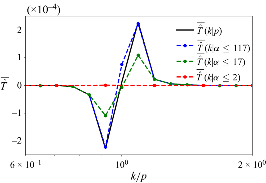
The figure shows  $\bar {\hat {T}} (k \vert p)$ for four different rotation rates for
 $k=200$, in the middle of the inertial range. The different panels are (a)
 $f=0$; (b)
 $f=1$; (c)
 $f=2$; (d)
 $f=3$. Observe that the magnitude of
 $\bar {\hat {T}} (k \vert p)$ reduces with increasing
 $f$, as a consequence of weakening of the transfers at higher rotating rates.

Although the above analysis reveals that the turbulent forward cascade of waves in RSWE is scale-local, non-local modes can be involved in the transfer. To see this, recall that in (3.3)  $\hat {S}(k \vert p, q, t)$ was summed over all
 $q$ wavenumbers to obtain
 $\hat {T} (k \vert p, t)$. Although the lengths of wavenumbers
 $k$ and
 $p$ can be comparable,
 $q$ can be of really small length resulting in
 $q \ll k \sim p$. Consequently, although the turbulent transfer is scale-local, there is nothing preventing widely separated or non-local wavenumbers affecting the turbulent transfer. To examine the possibility of non-local modes being involved in the transfer, we summed
 $\hat {S} (k \vert p, q, t)$ over selected wavenumbers
 $q$ as follows.
For a triad  $(k, p, q)$ contributing to the turbulent transfer, we define
 $\alpha = \text {max}(k, p, q)/\text {min}(k, p, q)$ as the ratio of the maximum to minimum wavenumber. In hydrodynamic turbulence a triad is considered to be local if
 $\alpha \leqslant 2$ and non-local if
 $\alpha > 2$ (Lesieur Reference Lesieur2008). We used
 $\alpha$ to compute the partial transfer function
 $\hat {T}(k \vert p; \alpha \leqslant m, t )$ as
 \begin{equation} \hat{T}(k \vert p; \alpha \leqslant m , t) = \sum_{q \ \text{such that } \alpha \leqslant m } \hat{S} (k \vert p, q, t), \end{equation}
where  $m$ is a number we set so that the summation on the right-hand side above can be computed subject to the constraint that only triads that fall within a certain value of length ratios are considered. For example, setting
 $m=2$ would give us the transfer function considering only local triads,
 $\hat {T}(k \vert p; \alpha \leqslant 2, t)$.
We computed  $\bar {\hat {T}} (k \vert p; \alpha \leqslant m)$, the time-averaged
 $\hat {T}(k \vert p; \alpha \leqslant m, t )$, for different
 $m$ values across different rotation rates and a plot that summarizes the main results of our analysis is shown in figure 7 for
 $f=1$. Notice that when we set
 $\alpha \leqslant 2$ (red curve in figure 7), which constrains the triads to local modes alone, we do not capture any part of the complete transfer function (black curve in figure 7). Setting
 $\alpha \leqslant 17$, which allows for non-local triads, results in the green curve in figure 7: notice that the green curve captures approximately 50 % of the maxima and minima of the total transfer function shown by the black curve. Finally, further increasing the non-locality of the modes and setting
 $\alpha \leqslant 117$ leads to the blue curve in figure 7, which captures most of the total transfer function shown by the black curve. This analysis reveals that non-local modes are crucial for obtaining the complete transfer function. Although
 $\bar {\hat {T}}$ itself shows highly localized behaviour, as seen in figure 6, non-local triads form an important part of
 $\bar {\hat {T}}$. We therefore conclude that the turbulent downscale transfer of waves in RSWE is a result of the interaction of non-local triads, although the transfer itself is scale-local. The same conclusion, i.e. local transfer due to non-local triads is a well established result in 3-D HIT (Domaradzki & Rogallo Reference Domaradzki and Rogallo1990; Yeung & Brasseur Reference Yeung and Brasseur1991; Ohkitani & Kida Reference Ohkitani and Kida1992; Waleffe Reference Waleffe1992; Zhou Reference Zhou1993; Brasseur & Wei Reference Brasseur and Wei1994; Domaradzki & Carati Reference Domaradzki and Carati2007; Eyink & Aluie Reference Eyink and Aluie2009; Cardesa, Vela-Martin & Jimenez Reference Cardesa, Vela-Martin and Jimenez2017). Our analysis reveal that the same feature is exhibited by the turbulent forward energy cascading inertia-gravity waves in RSWE.


3.3. Finite non-zero time delay in the cascade
As discussed before, the locality results seen in figure 6 required time averaging to remove fast fluctuations. An instantaneous snapshot of  $\hat {T}(k \vert p, t)$ did not give clear insights on locality of transfers, although the time-averaged or the slow part of
 $\hat {T}$ did. This is an indication that the slow energy transfers happen by scale-local transfers, although fast fluctuations associated with energy transfers do not necessarily adhere to locality constraints. Fast fluctuations in energy, transfer functions and fluxes were seen to be a generic feature of the turbulent transfers we examined. An example is shown in figure 8(a) where the time series of transfer function
 $\hat {R} (k, t)$ for different wavenumbers is plotted in an arbitrary time interval for
 $f=1$. Notice that the amplitude of oscillations is quite high for low wavenumbers, e.g.
 $k=20$, while they reduce with increasing wavenumbers and is relatively negligible at high wavenumbers, e.g.
 $k=200$.
Panel (a) shows the variation of  $\hat {R} (k, t)$ with time for different
 $k$ in an arbitrary time interval. Panels (b,d) show the correlation between
 $\hat {R} (k_1, t)$ and
 $\hat {R} (k_2, t + \tau )$, while (c,e) show the correlation between the slow part of the transfer functions,
 $\hat {R}_{s} (k_1, t)$ and
 $\hat {R}_{s} (k_2, t + \tau )$, respectively. Panel ( f) shows the variation of the maximum correlation curve, i.e. the white lines in (c,e) above, across the inertial range. Here (a)
 $f=1$; (b)
 $f=1$; (c)
 $f=1$; (d)
 $f=3$; (e)
 $f=3$.

Due to scale-local transfers, energy from large scales will not be able to reach small dissipative scales instantaneously by means of a direct transfer. Instead, a certain finite time is to be expected for energy to get transferred from large to small scales. One way to confirm this non-zero time delay is to compute the time-lag correlation between time series’ of domain-integrated energy and dissipation, as is often done in 3-D HIT investigations (see e.g. Cardesa et al. Reference Cardesa, Vela-Martin, Dong and Jimenez2015). Energy and dissipation may be considered as large-scale and small-scale variables, respectively, which means that their time correlation will inform us about the presence of a delay between the two signals. We computed the time-lag correlation between energy and dissipation for different rotation rates and for all cases found that the maximum correlation between the time series occur with a time lag, hinting at the delay in energy reaching dissipative scales from large domain scales. Here we skip a detailed discussion of these figures, the figures being similar to those seen in 3-D HIT studies, see for example figure 2 in Cardesa et al. (Reference Cardesa, Vela-Martin, Dong and Jimenez2015). For a more illuminating illustration of the time delay in the cascade process, we will now discuss results of an investigation we undertook inspired by the study of Khurshid, Donzis & Sreenivasan (Reference Khurshid, Donzis and Sreenivasan2021) for 3-D HIT, where the time delay between the transfer functions at different wavenumbers is examined.
We computed the time-lag correlation of  $\hat {R}$ across different wavenumbers, i.e. the correlation between
 $\hat {R} (k_1, t)$ and
 $\hat {R} (k_2, t + \tau )$, where
 $k_1$ was chosen to be 20, at large scales and a little away from the forced wavenumbers, and we increased
 $k_2$ starting from
 $k_1$ and went across the inertial range up to
 $k_2=600$, where dissipation starts to become non-negligible. Figures 8(b) and 8(d) show the correlation as a function of
 $k_2$ and the time lag
 $\tau$ for
 $f=1$ and
 $f=3$, respectively. Scanning through these figures reveals that not much correlation is seen across the inertial range. Following this, we performed a running time average on the transfer function
 $\hat {R}$ at different wavenumbers to remove the high frequency oscillatory part of the transfer function. The averaging window was chosen by trial and error and approximately 10 domain-scale wave periods was seen to be a sufficient time window for removing fast fluctuations and obtain
 $\hat {R}_{s}$, the slow component of the transfer function. We then computed the correlation between slow part of the transfer functions at different wavenumbers,
 $\hat {R}_{s} (k_1, t)$ and
 $\hat {R}_{s} (k_2, t + \tau )$, and the results for
 $f=1$ and
 $f=3$ are shown in figures 8(c) and 8(e). Notice that there is a clear correlation between the slow transfer functions across the inertial range, while there was no noticeable correlation between the full transfer functions. In figures 8(c) and 8(e), the maximum correlation curve is marked by a white line. These maximum correlation curves are separately replotted in figure 8( f). Notice that the time lag
 $\tau$ increases from
 $k_1=20$ and gradually reaches a saturation value in the inertial range. This behaviour confirms that the slow part of the transfer function is correlated across scales with a time lag, an indication of the time delay associated with the forward energy cascade. It is noteworthy that these results which we obtained for inertia-gravity waves in RSWE are synonymous with the results obtained for 3-D HIT by Khurshid et al. (Reference Khurshid, Donzis and Sreenivasan2021); see for instance their figures 1, 4 and 5. Therefore, just like in 3-D HIT, the turbulent downscale cascade of wave energy takes a certain time to reach dissipation scales from the domain scale, a result that is to be expected in hindsight since the downscale transfer is scale-local.
3.4. Temporal intermittency of energy transfers
As is clear from the discussions in §§ 3.2 and 3.3, the slow downscale energy transfer is scale-local and is associated with a finite time lag. The fast fluctuations on the other hand do not show noticeable correlations across scales and do not respect locality of transfers. Nevertheless, the fast fluctuations are associated with several features closely connected to temporal intermittency of transfers. Specifically, the temporal intermittency in transfers were seen to have close connections to physical structures and their time evolution, which we detail below.
For  $f=1$, figure 9(a) shows the time series of spatial maxima of pointwise dissipation,
 $D^\epsilon$, and pointwise negative divergence,
 $- \boldsymbol {\nabla } \boldsymbol {\cdot } \boldsymbol {v}$, for an arbitrary time interval. To plot these variables on the same figure we subtracted the mean of the time series from the instantaneous values and then divided the difference by the mean. On scanning figure 9(a), we notice that dissipation and negative divergence are in phase; notice that both of them attain high values at almost the same instances in time. In figure 9(b), we plotted the time series of spatial maxima of dissipation, i.e. the same black curve from figure 9(a), and the time series of energy flux at
 $k=200$, a wavenumber in the middle of the inertial range. Similar to the other curves in figure 9, we subtracted the mean flux from the instantaneous flux values and normalized by the mean flux to get the blue flux curve plotted in figure 9(b). The three different time series shown in figure 9 indicate that the variables fluctuate intermittently with time, with different local maxima. For convenient viewing we used a grey shading for different regions in figure 9(b) that contains local maxima of the variables. A reader who carefully examines figure 9(b) will notice that the local maxima of flux precedes the local maxima of dissipation; this feature can be seen in each grey shaded region of the figure, starting with the first maxima happening after
 $t = t_{1} + 2.5$. The flux attaining a maxima before the maxima of dissipation and negative divergence is another explicit illustration of the results discussed in § 3.3; i.e. the finite non-zero time associated with energy cascading across the inertial range to the dissipative scales.
Panel (a) shows the time variation of pointwise spatial maximum of dissipation ( $D^\epsilon _{max}$) and negative divergence (
 $- { ( \boldsymbol {\nabla } \boldsymbol {\cdot } \boldsymbol {v} )}_{min}$). Panel (b) shows the time variation of pointwise spatial maximum of dissipation and energy flux at
 $k=200$. The inset in (a) shows the zoomed view of the region marked by the dashed blue lines in (a). The black dots in the top-right inset are chosen times at which the physical fields in figure 10 are shown. The first local maximum of the negative divergence happens at
 $t = t_{1} + 2.81$, this corresponding to the topmost black dot in the inset.

Alongside tracking the temporal fluctuations seen in figure 9, we monitored the details in physical space structures at different times. A key result was the finding that the local maxima of flux, negative divergence and dissipation went hand-in-hand with the intersection of a large number of shocks in physical space. To illustrate this, the inset at the top right-hand side of figure 9(a) shows a small part of the time series that is highlighted by the dashed blue lines in the bottom left of figure 9(a). In the inset we have marked five specific time instances by black dots, two before and two after the local maxima at  $t = t_{1} + 2.81$. The physical space structures of the log of the absolute value of divergence and dissipation corresponding to these five time instances are shown in figure 10. A specific region of interest is highlighted by white dashed boxes in figure 10. On carefully examining figure 10 from figure 10(a,b) to figure 10(i,j), especially focusing on the region inside the white dashed boxes, the reader will find that different shocks move across the domain and intersect at specific locations. An incident that stands out is seen in figure 10(e,f), corresponding to
 $t = t_{1} + 2.81$, where twelve shocks intersect at a location where the maxima of negative divergence and dissipation are attained, these being seen in the inset of figure 9(a). Notice that the moving shocks converge to this point in space before this time instant and diverge from each other after this time instant. We found this feature to be persistent for different local maxima of the curves seen in the grey shaded regions of figure 9. Local maxima of flux, dissipation and negative divergence correspond to a large number of shocks intersecting in physical space, with their intersection being the location of maxima of dissipation and negative divergence.
The figure shows the  $\log$ of the absolute value of the divergence field,
 $\boldsymbol {\nabla } \boldsymbol {\cdot } \boldsymbol {v}$, (a,c,e,g,i) and the dissipation field,
 $D^\epsilon$, (b,d,f,h,j) at different times, corresponding to the times marked by black dots in the inset of figure 9(a). The dashed white boxes in the panels above highlight a specific region where a large number of shocks meet at
 $t = t_{1} + 2.81$, this being the time at which pointwise negative divergence and pointwise dissipation attain the maximum values, once again as seen from the top-most black dot at
 $t = t_{1} + 2.81$ in the inset of figure 9(a). Shocks move towards this intersection point at earlier times and shocks move away from this intersection point at later times, as can be seen by examining the dashed white box at different times from (a,b) to (i,j). Here (a,b)
 $t = t_{1} + 2.45$; (c,d)
 $t = t_{1} + 2.62$; (e,f)
 $t = t_{1} + 2.81$; (g,h)
 $t = t_{1} + 2.95$; (i,j)
 $t = t_{1} + 3.46$.

The above-described features were also seen for the other rotation rates and a key finding was that the level of intermittency increased with increasing rotation rate. To illustrate this, figure 11 shows the spectral flux for the  $f=1$ case and
 $f=3$ case, the former shown in figure 11(a) and is the same blue curve that appears in figure 9(b). Notice that while we see multiple flux bursts from the mean for the
 $f=1$ case, only one distinguished burst in flux is seen for the
 $f=3$ case in figure 11(b) in the same time interval. Furthermore, the single burst seen in
 $f=3$ case is of much higher amplitude than that of the
 $f=1$ case. We noticed this to be a distinguishing feature of the turbulent transfers with increasing rotation rates: higher rotation rates were associated less frequent but larger amplitude bursts in flux, this being followed by multiple shocks intersecting in the domain and high dissipation and negative divergence values at the intersection points.
Figure shows the time variation of the spectral flux at  $k=200$ for (a)
 $f = 1$ and (b)
 $f = 3$. Panel (a) shows the same blue curve in figure 9(b), replotted above for a convenient comparison.

We conclude this section by noting that the turbulent wave transfers are in general intermittent in time, with the temporal intermittent behaviour being correlated with distinguished features in the physical domain and with the temporal intermittency of the signals increasing with increase in the rotation rate.
4. Turbulent wave cascade in the presence of a vortical flow
So far we examined features of the wave cascade in the absence of the vortical flow. In this section we will briefly discuss the effect of the vortical mode on the waves’ cascade. We initialized a vortical flow by choosing a random field in spectral space restricted to  $k \leqslant 5$ such that the initial conditions satisfied the vortical equations, (2.5), and such that the domain-averaged vortical energy was unity, i.e.
 ${{E}_{\scriptscriptstyle {V}}} (t=0)/A =1$. The wave field was not initialized and we let the vortical field evolve into a fully developed stage by integrating up to
 $t=50$. During the initial transient phase when spectral broadening of the vortical flow took place, we found that the flow lost approximately 1 %–2 % of the initial energy. For example, for
 $f=1$ and
 $f=5$ cases, we found that the vortical flow's domain-averaged energy dropped from 1 to 0.9892 and 0.9974, respectively, during the short initial transient phase when the spectrum developed. Beyond this short transient phase the vortical dissipation was seen to be negligible, once the flow was fully developed and figure 12 shows a snapshot of the potential vorticity field, discussed below (2.6a,b), and the energy spectrum of the vortical mode as an example for the
 $f=5$ case at
 $t=50$. For all rotation rates
 $t=50$ was seen to be long enough for a vortical spectrum to develop, as seen from the example case in figure 12(b).
(a) Potential vorticity and (b) energy spectrum of the vortical field for  $f=5$.

At  $t=50$ we stopped the numerical integration and constructed a random flow of linear waves at low wavenumbers,
 $k \leqslant 5$, with unit domain-averaged wave energy, i.e.
 ${{E}_{\scriptscriptstyle {W}}} (t=0)/A =1$. We then reinitialized the flow such that the new flow field was the sum of the random low wavenumber wave field and the well-developed vortical field from the previously stopped numerical integration. This initialization ensured that both wave and vortical flow had comparable energy levels, with domain-averaged wave energy being unity and domain-averaged vortical energy being 1 %–2 % less than unity. The RSWE was then again time-integrated with this initialization, with waves being forced at low wavenumbers as in the previous section but with no vortical forcing. This integration continued from
 $t=50$ to
 $t=170$. The time series of the total energy for different rotation rates can be seen in figure 1(b): notice the first integration from
 $t=0\unicode{x2013}50$ where the vortical flow is evolved and the second phase from
 $t=50\unicode{x2013}170$ where waves and the vortical flow are evolved. We discarded solutions from
 $t=50\unicode{x2013}90$ and used flow fields from
 $t=90\unicode{x2013}170$ for the results presented below, including the time-averaged statistics. Table 2 shows the Rossby number, different energies and dissipation, and the change in the vortical energy in the interval
 $t=90\unicode{x2013}170$.
Figure 13(a) shows the waves’ energy spectra in the presence of the vortical field (solid lines) and in the absence of the vortical field (dashed lines). The dashed lines are identical to those appearing in figure 3(a) and are replotted here for a convenient comparison. On comparing the solid and dashed lines in figure 13(a), we find that at low rotation rates the waves’ spectra are not much different with and without the vortical field. On the other hand, at high rotation rates the wave spectrum is much shallower in the presence of the vortical field, see for instance the  $f=5$ spectrum. The vortical field scatters the wave energy to small scales and thereby increases the wave energy at small scales. This inference is visually confirmed by comparing the divergence field with and without the vortical field. Figure 2(b,d,f,h) shows the negative divergence of the flow velocity field in the presence of the vortical field while figure 2(a,c,e,g), discussed earlier, shows the divergence field in the absence of the vortical field. For
 $f=1$, the shock strength looks similar on figure 2(a) and figure 2(b), although we notice that the shocks are more curved in figure 2(b), a result of scattering of waves by the vortical field. For the
 $f=2$ case, it is clear that the shock strength is higher for the flow with the vortical mode. Similar inference holds for
 $f=3$ case. For the
 $f=5$ case, we see that in figure 2(g) that there is no sign of shock formation: the high rotation rate halts the forward cascade of waves. In contrast, figure 2(h) for
 $f=5$ case shows the formation of shocks. The physical field visualizations indicate that the vortical flow can scatter waves and lead to shock formation even in fast rotating flows where waves do not form shocks in the absence of the vortical flow, thereby increasing the wave energy content at small scales as seen in the waves’ energy spectra in figure 13(a).
Panel (a) shows the waves’ spectra for different  $f$ with the vortical field (solid lines,
 $V \neq 0$) and without the vortical field (dashed lines,
 $V \approx 0$), while panel (b) shows the time-averaged waves’ flux for the case
 $f=5$.

To examine the effect of vortical scattering on waves, we will now look at the energy fluxes. The waves’ spectral energy equation is given by
 \begin{equation} \frac{{\rm d}{ }}{{\rm d}{t}} { \hat{E}_W (k, t) } = \underbrace{\hat{R}_{WWW} (k, t) + \hat{R}_{WVW} (k, t) + \hat{R}_{WVV} (k, t)}_{\hat{R}_W (k, t)}\, , \end{equation}
where  $\hat {E}_W (k, t)$ is the wave energy at a given wavenumber
 $k$ defined in (2.9) and the transfer function
 $\hat {R}_W (k, t)$ denotes the rate of change of energy at wavenumber
 $k$ due to triadic nonlinear interactions between waves alone, denoted by the WWW term, and wave–vortex interactions: wave–vortex–wave (WVW) and wave–vortex–vortex (WVV). Since waves form a high frequency mode and the vortical flow is a low frequency mode, two wave modes can resonantly interact with a vortical mode acting as a catalyst. As a result, the WVW term above is often identified as a resonant triadic interaction term. On the other hand, two vortical modes cannot interact with a wave mode by resonant interactions and consequently the WVV term is often identified as a non-resonant triadic interaction term. We refer an interested reader to Majda (Reference Majda2002), Ward & Dewar (Reference Ward and Dewar2010) and Remmel & Smith (Reference Remmel and Smith2009) for more details on these resonant, near-resonant and non-resonant interactions, along with specific asymptotic calculation examples for different kinds of interactions.
Recalling energy equations discussed in the previous section, at this point it is useful to make a connection to (3.1). The above equation, (4.1), is the wave energy equation which is needed to examine the energy transfers associated with waves. On the other hand, (3.1) is the total energy equation, which matches with the wave energy equation since the vortical energy was insignificant for the cases we discussed in § 3. For our present discussions on flows involving wave and vortical flow, it is necessary to write an explicit wave energy equation as in (4.1), since the total energy equation captures energy changes of both the wave and the vortical field.
We obtain the wave energy flux equation by summing (4.1) over wavenumbers from  $k_{max}$ to
 $k$ as
 \begin{equation} \frac{{\rm d}{ }}{{\rm d}{t}} \sum_{p=k_{max}}^{p=k} \hat{E}_W (p, t) = \underbrace{ \hat{\varPi}_{WWW} (k, t) + \hat{\varPi}_{WVW} (k, t) + \hat{\varPi}_{WVV} (k, t)}_{ \hat{\varPi}_W (k, t)}\, , \end{equation}
where  $\hat {\varPi }_W (k, t)$ represents the wave energy flux, which is again decomposed into different components based on the kind of nonlinear interactions.
We looked at the waves’ flux and its components given in (4.2) for different rotation rates and found that at low rotation rates the waves’ flux  $\hat {\varPi }_W$ was comparable for cases with and without the vortical field. More specifically, at low rotation rates the triadic wave interaction term,
 $\hat {\varPi }_{WWW}$, dominated the wave flux while the flux terms that contained the vortical mode,
 $\hat {\varPi }_{WVW}$ was negligible. However, as rotation rate increased, the resonant
 $\hat {\varPi }_{WVW}$ term became significant. At all rotation rates, the non-resonant
 $\hat {\varPi }_{WVV}$ term was seen to be insignificant. An example is shown in figure 13(b), where the time-averaged flux and its decomposition is presented for the
 $f=5$ case. Notice that the resonant
 $\bar {\hat {\varPi }}_{WVW}$ in figure 13(b) is comparable to the
 $\bar {\hat {\varPi }}_{WWW}$, thereby contributing to the total waves’ forward flux term
 $\bar {\hat {\varPi }}_{W}$. Also observe that the non-resonant term
 $\bar {\hat {\varPi }}_{WVV}$ is extremely weak and contributes very little.
It is interesting that the vortical flow has little role on the waves’ forward cascade at low rotation rates. The forward cascade rates of the wave field due to triadic wave interactions, dictated by the  $\hat {\varPi }_{WWW}$ term, is dominant at low rotation rates, while the
 $\hat {\varPi }_{WVW}$ term representing scattering of the wave field by the vortical field is relatively weak. In other words, nonlinear interactions between waves are much stronger than vortical scattering of waves at low rotation rates and the waves’ forward cascade has little contribution from vortical scattering. With increasing rotation rate triadic wave interactions weaken, eventually reaching a point where the
 $\hat {\varPi }_{WWW}$ term and the
 $\hat {\varPi }_{WVW}$ term becomes comparable, as seen in the figure 13(b). At such high rotation rates, vortical scattering of the wave field plays a major role in the forward cascade of the wave field.
The increased effect of the vortical scattering of wave energy to smaller scales leads to higher dissipation in flows that contain a vortical field when compared with flows that do not contain a vortical flow. This inference can be made by comparing the last two columns of table 1, that lists dissipation, with the corresponding columns in table 2. We see that dissipation values in table 2 are higher than those in table 1 by orders of magnitude at high rotation rates, this being a reflection of the role the vortical field plays in scattering and downscale flux of wave energy.
The above discussion of energy flux points out that the vortical mode assists in the waves’ forward cascade, specifically via the WVW term. To further get a handle on the regions in the vortical flow that assist in the waves’ forward cascade, we divided the flow domain into strain-dominant and vorticity-dominant regions based on the Okubo–Weiss criterion (Okubo Reference Okubo1970; Weiss Reference Weiss1991). Given the vortical velocity field  $({{u}_{\scriptscriptstyle {V}}}, {{v}_{\scriptscriptstyle {V}}})$, the normal strain rate and the shear strain rate were computed as
 $\sigma _n = \partial {{u}_{\scriptscriptstyle {V}}}/\partial x - \partial {{v}_{\scriptscriptstyle {V}}}/ \partial y$ and
 $\sigma _s = \partial {{v}_{\scriptscriptstyle {V}}}/\partial x + \partial {{u}_{\scriptscriptstyle {V}}}/ \partial y$, respectively. These components were then used to find the total strain rate due to the vortical field,
 ${{ \sigma }_{\scriptscriptstyle {V}}} = \sqrt { \sigma _n^2 + \sigma _s^2}$. Figure 14(a,b) show the vorticity,
 ${{ \zeta }_{\scriptscriptstyle {V}}}$, and strain,
 ${{ \sigma }_{\scriptscriptstyle {V}}}$, respectively, associated with the vortical mode for
 $f=5$ case. Carefully comparing these two figures, the reader will notice that vorticity is high in the core of the coherent vortices while strain rate is high at the boundaries of coherent vortices. Vorticity-dominant regions with
 ${{ \sigma }_{\scriptscriptstyle {V}}} < \vert {{ \zeta }_{\scriptscriptstyle {V}}} \vert$ are therefore regions in the core of coherent vortices while strain-dominant regions with
 ${{ \sigma }_{\scriptscriptstyle {V}}} > \vert {{ \zeta }_{\scriptscriptstyle {V}}} \vert$ are regions around the boundaries of the coherent vortices.
The figure shows results for  $f=5$ case. Panels (a,b) show the vorticity,
 $\zeta_V$, and strain rate,
 $\sigma_V$, associated with the vortical field, while (c) shows the waves’ flux term
 $\bar {\hat {\varPi }}_{WVW}$ and its decomposition into contributions from strain-dominant and vorticity-dominant regions.

We then decomposed the vortical flow fields into parts that correspond to strain-dominant and vorticity-dominant regions. For example, the vortical velocity in the  $x$-direction was decomposed as
 ${{u}_{\scriptscriptstyle {V}}} = u_{\scriptscriptstyle {V} }^{\scriptscriptstyle {({{ \sigma }_{\scriptscriptstyle {V}}} > \vert {{ \zeta }_{\scriptscriptstyle {V}}} \vert )}} + u_{\scriptscriptstyle {V} }^{\scriptscriptstyle {({{ \sigma }_{\scriptscriptstyle {V}}} < \vert {{ \zeta }_{\scriptscriptstyle {V}}} \vert )}}$ such that
 \begin{equation} u_{\scriptscriptstyle {V} }^{\scriptscriptstyle {\left({{ \sigma}_{\scriptscriptstyle{V}}} > \vert {{ \zeta}_{\scriptscriptstyle{V}}} \vert \right)}} = \begin{cases} u_{\scriptscriptstyle {V} } & \text{for} \ {{ \sigma}_{\scriptscriptstyle{V}}} > \vert {{ \zeta}_{\scriptscriptstyle{V}}} \vert \\ 0 & \text{for} \ {{ \sigma}_{\scriptscriptstyle{V}}} < \vert {{ \zeta}_{\scriptscriptstyle{V}}} \vert \end{cases}\quad\text{and}\quad u_{\scriptscriptstyle {V} }^{\scriptscriptstyle {\left({{ \sigma}_{\scriptscriptstyle{V}}} < \vert {{ \zeta}_{\scriptscriptstyle{V}}} \vert \right)}} = \begin{cases} u_{\scriptscriptstyle {V} } & \text{for} \ {{ \sigma}_{\scriptscriptstyle{V}}} < \vert {{ \zeta}_{\scriptscriptstyle{V}}} \vert \\ 0 & \text{for} \ {{ \sigma}_{\scriptscriptstyle{V}}} > \vert {{ \zeta}_{\scriptscriptstyle{V}}} \vert \end{cases}. \end{equation}
In the above decomposition,  $u_{\scriptscriptstyle {V} }^{\scriptscriptstyle {({{ \sigma }_{\scriptscriptstyle {V}}} > \vert {{ \zeta }_{\scriptscriptstyle {V}}} \vert )}}$ was obtained by setting
 $u_{\scriptscriptstyle {V} }$ to zero at physical points where
 ${{ \sigma }_{\scriptscriptstyle {V}}} < \vert {{ \zeta }_{\scriptscriptstyle {V}}} \vert$. A similar procedure was followed to obtain
 $u_{\scriptscriptstyle {V} }^{\scriptscriptstyle {({{ \sigma }_{\scriptscriptstyle {V}}} < \vert {{ \zeta }_{\scriptscriptstyle {V}}} \vert )}}$. We maintained strict inequality to obtain these regions, since it was seen that the contribution from regions that satisfy the equality
 ${{ \sigma }_{\scriptscriptstyle {V}}} = \vert {{ \zeta }_{\scriptscriptstyle {V}}} \vert$ was insignificant. We then used these decomposed fields to decompose the flux component as
 \begin{equation} \hat{\varPi}_{WVW} = \hat{\varPi}_{WVW}^{\scriptscriptstyle {\left({{ \sigma}_{\scriptscriptstyle{V}}} > \vert {{ \zeta}_{\scriptscriptstyle{V}}} \vert \right)}} + \hat{\varPi}_{WVW}^{\scriptscriptstyle {\left({{ \sigma}_{\scriptscriptstyle{V}}} < \vert {{ \zeta}_{\scriptscriptstyle{V}}} \vert \right)}}, \end{equation}
where  $\hat {\varPi }_{WVW}^{\scriptscriptstyle {({{ \sigma }_{\scriptscriptstyle {V}}} > \vert {{ \zeta }_{\scriptscriptstyle {V}}} \vert )}}$ was computed using the vortical flow fields that correspond to strain-dominant regions while
 $\hat {\varPi }_{WVW}^{\scriptscriptstyle {({{ \sigma }_{\scriptscriptstyle {V}}} < \vert {{ \zeta }_{\scriptscriptstyle {V}}} \vert )}}$ used the vortical flow fields corresponding to vorticity-dominant regions.
Figure 14(c) shows the contribution of the decomposed flux terms on the right-hand side of (4.4). Notice that the flux contribution from the strain-dominant regions is higher than the flux contribution from vorticity-dominant regions, which in turn implies that the boundary regions around coherent vortices play a bigger role in catalyzing the forward cascade of waves in comparison with the coherent vortex cores.
The results discussed above indicate that the vortical field can enhance the forward cascade of waves, an effect whose importance increases at higher rotation rates. Visually, this effect strikingly stands out in figure 2(g,h) showing the negative divergence field of the  $f=5$ flow with and without the vortical flow. The flow with waves alone have no signs of shocks, while the flow with a vortical mode and waves show shocks, this being a result of the vortical scattering of waves. Returning to our discussion in the introduction, recall that the asymptotic resonant wave interaction theory in the weakly nonlinear regime predicts that vortical scattering of waves maintains the scale of the waves (Majda Reference Majda2002; Ward & Dewar Reference Ward and Dewar2010). More specifically, a wave of wavenumber magnitude
 $k$ and frequency
 $\omega =\sqrt {f^2 + k^2}$ can exchange energy with another wave with the same wavenumber magnitude and frequency. Within the context of the asymptotic theory, this WVW triadic resonant interaction does not change the scale of the wave, since the wavenumber magnitude of the interacting waves remain the same. However, as seen in our results above, the vortical mode can scatter waves and generate smaller scale waves that cascade wave energy downscale via the
 $\hat {\varPi }_{WVW}$ flux term. The result indicates that the inertia-gravity waves in RSWE exhibit dynamics that are indeed beyond the predictions of resonant wave interaction theory.
We also note that the features of the waves’ forward cascade discussed in § 3 in the absence of the vortical flow were also seen in the presence of the vortical flow. For instance, locality of transfers, finite and non-zero time lag associated with the wave energy moving across the inertial range, and temporal intermittency and its repercussions in spectral space and physical space detailed in the previous section were seen to be qualitatively similar in the presence of the vortical field. We omit these figures here to avoid repetition and end by noting that the primary effect of the vortical mode on waves is that the vortical mode can scatter waves and enhance the waves’ forward cascade, generating shallower waves’ spectra and more small-scale structures and shock in physical space. These effects are more pronounced at high rotation rates; at low rotation rates waves’ scattering by the vortical mode primarily makes the shocks more curved.
4.1. Wave-balance energy exchanges
Applying the wave-balance decomposition to RSWE (2.3) with the dissipation term on the right-hand side, we get the evolution equation for the vortical flow variables. Taking the Fourier transform of those equations we can form the energy of the vortical flow as
 \begin{equation} \frac{\partial{ {{\hat{E} }_{\scriptscriptstyle{V}}} (\boldsymbol{k}, t) }}{\partial{t}} = {{ \hat{R}}_{\scriptscriptstyle{V}}} (\boldsymbol{k}, t) - {{ \hat{D}}_{\scriptscriptstyle{V}}} ( \boldsymbol{k}, t), \end{equation}
where the quadratic vortical energy is given by  ${{ \hat {E} }_{\scriptscriptstyle {V}}} (\boldsymbol {k}, t) = \vert {{ \hat {u}}_{\scriptscriptstyle {V}}} (\boldsymbol {k}, t) \vert ^2 + \vert {{ \hat {v}}_{\scriptscriptstyle {V}}} ( \boldsymbol {k}, t) \vert ^2 + \vert {{ \hat {h}}_{\scriptscriptstyle {V}}} ( \boldsymbol {k}, t) \vert ^2$ and the corresponding dissipation is given by
 ${{\hat D}_{\scriptscriptstyle {V}}} (\boldsymbol {k}, t) = \nu \boldsymbol {k}^4 {{ \hat {E} }_{\scriptscriptstyle {V}}} (\boldsymbol {k}, t)$. Additionally,
 ${{ \hat {R}}_{\scriptscriptstyle {V}}}$ is the nonlinear transfer term that is responsible for energy exchanges. This term is similar to the
 ${{ \hat {R}}_{\scriptscriptstyle {W}}}$ term in (4.1), although unlike in (4.1) here we do not further decompose the term into different triadic contributions. Summing the above equation over all wavenumbers gives us the domain-integrated energy equation for the vortical flow as
 \begin{equation} \frac{{\rm d}{ {{E}_{\scriptscriptstyle{V}}} (t) }}{{\rm d}{t}} = {{R}_{\scriptscriptstyle{V}}} ( t) - {{D}_{\scriptscriptstyle{V}}} ( t). \end{equation}
As explained earlier, we used the equilibrated fields from  $t=90\unicode{x2013}170$ to compute all the transfers and statistics described so far. During this same interval, we time-integrated the right-hand side terms in (4.6) to get the change in the vortical energy during the time interval
 $t=90\unicode{x2013}170$. For example, we found this energy change per unit area for the
 $f=1$ case to be
 $\delta {{E}_{\scriptscriptstyle {V}}}/A = 0.0117$, almost two orders lower than the vortical energy per unit area, which is close to 1. This drop in vortical energy is reported in the last column of table 2 for different rotation rates. From the table we see that the energy exchange with the wave field and vortical dissipation is negligible, leading to vortical energy changing very little during our numerical integrations. This is why we did not have to force the vortical field in our numerical integrations, although we forced the wave field.
The above discussion points out how weak energy exchange is between waves and vortical modes in the regime considered here for RSWE, where wave and vortical modes are comparable in strength. In the past, a broad set of studies have examined wave-balance energy exchanges in different contexts using asymptotic models, two-dimensional and 3-D models (Gertz & Straub Reference Gertz and Straub2009; Xie & Vanneste Reference Xie and Vanneste2015; Taylor & Straub Reference Taylor and Straub2016; Wagner & Young Reference Wagner and Young2016; Rocha, Wagner & Young Reference Rocha, Wagner and Young2018; Thomas & Yamada Reference Thomas and Yamada2019; Thomas & Arun Reference Thomas and Arun2020; Thomas & Daniel Reference Thomas and Daniel2020; Taylor & Straub Reference Taylor and Straub2020; Xie Reference Xie2020; Thomas & Daniel Reference Thomas and Daniel2021; Zhang & Xie Reference Zhang and Xie2023). These studies were primarily inspired by the need to identify whether different wave fields such as internal tides, near-inertial waves and internal wave continuum could act as an energy sink for oceanic balanced flow and the results and their consequences are reviewed in detail in Thomas (Reference Thomas2023). Based on the results from these studies, noticeable energetic interactions between waves and balanced flow of comparable strength is seen only in the case of small Burger number near-inertial waves. Other wave fields, like internal tides and internal wave continuum are seen to have negligible energy exchange with the balanced flow in regimes when the two fields have comparable strengths.
Based on the scaling we used in (2.2a–e), the Burger number,  $Bu$, for the flow regimes is
 $Bu =(c_0/fL)^2 \sim O(1)$, this being the case for low mode internal tides. As a result, amongst the broad set of studies that have examined wave-balance energy exchanges mentioned above, energy exchanges examined by Thomas & Yamada (Reference Thomas and Yamada2019) in the
 $Bu \sim O(1)$ regime using a two-vertical-mode model that is similar to RSWE, where waves did not form shocks, is the closest to the energy exchange discussions in our present work. In that study, it was seen that in parameter regimes where waves and balanced flow have comparable strengths, the energy exchange between the two fields was negligible. In the present study, we explored interactions between waves and the vortical field in the regime where the two fields had comparable energy levels, since this is the regime where vortical scattering of waves is strongest and our goal was to examine how the vortical flow affects the waves’ downscale cascade. If we made the vortical energy weaker than waves, there would be less scattering of waves by the vortical flow and less modification of the waves’ cascade by the vortical flow. Consequently, we conclude by noting that the primary role of the vortical mode in the regime where wave and balanced energy levels are comparable is to scatter waves to smaller scales, with negligible energy exchange with the waves.
5. Summary and discussion
In this paper we explored some of the features associated with the turbulent cascade of inertia-gravity waves in the weakly nonlinear regime of RSWE. Despite being a popular model for geophysical fluid flow applications, a disproportionately large set of investigations of RSWE have examined the turbulent dynamics of the geostrophic balanced vortical flow, leaving several interesting aspects of inertia-gravity wave turbulence unexplored. Inertia-gravity waves in RSWE are dispersive in nature, as a result of rotation. Consequently, in the weakly nonlinear regime one might anticipate wave dynamics to be dictated by resonant interactions. However, like in the case of compressible flows, inertia-gravity waves in RSWE can steepen and form shocks. Our present work was aimed at understanding the effect of rotation rate and the vortical flow on the turbulent dynamics of dispersive inertia-gravity waves that have a tendency to form shocks.
We found that the rotation rate had a direct effect on the waves’ turbulent dynamics. The non-rotating and the low rotating regimes were characterized by a strong forward cascade of wave energy,  $k^{-2}$ energy spectra, and a physical space composed of a rich distribution of shocks. Increasing rotation rate was seen to weaken the forward energy flux of waves, resulting in steeper waves’ energy spectra and decreased shock strength in physical space. With further increase in rotation rate, the waves’ cascade halted with insignificant energy transfer to small dissipative scales. Linear dispersive waves simply moved around in physical space with no sign of steepening and forming shocks.
In hindsight, an interesting yet unanticipated outcome of this study was the finding that the turbulent cascade of inertia-gravity waves in RSWE has some similarities with the turbulent flow cascade in 3-D HIT. Specifically, we found that the forward cascade of waves took place via local transfers while non-local modes contributed to the transfer. The locality of the turbulent transfer implies that a finite non-zero time lag is to be expected for energy to go from domain scale to dissipative scale. We were able to identify a time delay for wave energy to cascade across the inertial range. Both these features of the turbulent cascade, i.e. local transfers via non-local interactions and the time delay for the energy to cascade across the inertial range are well established features of the turbulent energy cascade in 3-D HIT.
We also found the turbulent wave transfers to be intermittent in time. The spectral energy flux, spatial maximum of dissipation and negative divergence in the physical domain were all seen to fluctuate in time. Energy flux maxima were followed by spatial maxima of dissipation and negative divergence in specific locations in the physical domain. On tracking these locations, we found that the spatial maxima of dissipation and negative divergence were located where a large number of shocks intersected in physical space. Shocks moved towards this location at earlier times and shocks moved away from each other at later times, with the time of intersection of many shocks succeeding the maxima of the energy flux in spectral space. The intermittency of the turbulent wave transfers therefore had interesting connections between spectral space and physical space features.
On introducing a vortical field into the domain along with waves, we found the above-mentioned features to be the same, apart from minor quantitative features. The major difference, however, was that vortices could scatter waves and thereby assist in the forward cascade of waves. The effect of the vortical field was not much felt at low rotation rates, where the scattering by the vortical flow primarily made the shocks more curved. However, the presence of the vortical flow made a major difference at high rotation rates. For instance, while fast rotating flows with waves alone and no vortical field lacked a forward wave cascade and shock formation, introducing the vortical field resulted in vortices scattering waves, enhancing the forward cascade of waves and thereby generating shallower waves’ spectra with more small-scale waves, resulting in the formation of multiple shocks in the physical domain.
Our results detailed above highlight several intricate features of dispersive inertia-gravity wave turbulence. Despite operating in the weakly nonlinear regime, much of the results we found are outside the scope of resonant wave interaction theory. For interactions involving waves alone, the dispersion relationship of inertia-gravity waves in RSWE does not allow resonant triads. As a result, four wave resonances are needed for wave interactions, making the downscale wave energy transfers much slower (see, for example, four wave interaction based upscale transfer results discussed in Thomas & Ding (Reference Thomas and Ding2023)). However, inertia-gravity waves steepen and form shocks, resulting in fast downscale transfers violating resonant-wave-interaction-theory-based results. A similar feature was seen in the presence of the vortical flow. Resonant wave interaction theory predicts that vortical scattering of waves cannot change the spatial scale of waves since the wavenumber of waves being scattered by a vortical mode remain the same. In contrast, numerical integration results revealed that scattering by vortices can enhance downscale transfer of waves by transferring wave energy to small-scale waves. Consequently, although we were based in the weakly nonlinear regime, the results we obtained point out key features associated with turbulent inertia-gravity wave dynamics that are outside the realm of resonant wave interaction theory.
In summary, we conclude by noting that RSWE is an intriguing model where dispersive wave turbulence in the system has different dynamics in the inverse and forward flux regimes. While the inverse flux regime is dictated by resonant wave interactions and is therefore composed of slow wave transfers (Thomas & Ding Reference Thomas and Ding2023), the forward cascade dynamics of waves is much faster and is not captured by asymptotic resonant wave interaction theory. The wave-steepening and shock-forming tendency of the equations is primarily responsible for the limited applicability of resonant wave interaction theory to the forward cascading waves in RSWE even in the weakly nonlinear regime.
Acknowledgements
The authors thank the reviewers for their comments and suggestions, which improved the presentation of the results in this paper.
Funding
J.T. acknowledges financial support from the Science and Engineering Research Board (SERB) of India through the project SRG/2022/001071 and the Deep Ocean Mission scheme of the Ministry of Earth Sciences (MoES) through the project F.No.MoES/PAMC/DOM/18/2022 (E-12926). P.G. acknowledges partial funding from New Faculty Seed Grant, IRD, IIT Delhi and partial funding from SERB through the project SRG/2022/000728.
Declaration of interests
The authors report no conflict of interest.
Appendix A. Forcing scheme
Here we detail the forcing scheme used to inject waves into the flow at large scales. We did not explicitly add a forcing term in the governing equations. Instead, the amplitude of velocity and height perturbations at small wavenumbers are rescaled to simulate permanence of large length scales. This forcing scheme is similar to that used in compressible flow equations discussed in Jossy & Gupta (Reference Jossy and Gupta2023).
The forcing scheme maintained a constant energy level in the forcing band of wavenumbers, which we will denote as  $\mathcal {K}^f = \{\boldsymbol {k} : k_1 \leqslant |\boldsymbol {k} | < k_2\}$. We did so by splitting the forcing band into smaller partitions
 $\mathcal {K}^f_i$ such that
 $\mathcal {K}^f_i = \{\boldsymbol {k} : k_i - 1/2 \leqslant |\boldsymbol {k}| < k_i + 1/2\}$ where
 $k_1 \leqslant k_i < k_2$, except for the first partition. As explained in the discussion of wavenumber partitions with regards to energy spectra in figure 3(a), we let the first partition be
 $0 \leqslant k < 0.5$. Let the quadratic wave energy in each partition be defined as
 \begin{equation} {{\hat{E}}_{\scriptscriptstyle{W}}} (\mathcal{K}^f_i) = \sum_{ \boldsymbol{k} \in \mathcal{K}^f_i } \left( |{{\hat{u}}_{\scriptscriptstyle{W}}}|^2 +|{{\hat{v}}_{\scriptscriptstyle{W}}}|^2 + |{{\hat{h}}_{\scriptscriptstyle{W}}}|^2 \right), \end{equation}
where for convenience we temporarily suppress the time dependence of the variables above. We further denote the total wave energy in the forcing band as  $e^2$, i.e.
 \begin{equation} \sum_i {{\hat{E}}_{\scriptscriptstyle{W}}} (\mathcal{K}^f_i) = e^2. \end{equation}
Let the forcing band be divided into a total number of  $N$ partitions. In the beginning of each time step, the variables in each partition
 $\mathcal {K}^f_i$:
 ${{\hat {u}}_{\scriptscriptstyle {W}}} (\mathcal {K}^f_i)$,
 ${{\hat {v}}_{\scriptscriptstyle {W}}} (\mathcal {K}^f_i)$ and
 ${{\hat {h}}_{\scriptscriptstyle {W}}} (\mathcal {K}^f_i)$ are rescaled to
 ${{ \tilde {\hat {u}} }_{\scriptscriptstyle {W}}} (\mathcal {K}^f_i)$,
 ${{ \tilde {\hat {v}} }_{\scriptscriptstyle {W}}} (\mathcal {K}^f_i)$ and
 ${{\tilde {\hat {h}} }_{\scriptscriptstyle {W}}} (\mathcal {K}^f_i)$, such that
 \begin{equation} \left( {{ \tilde {\hat{u}} }_{\scriptscriptstyle{W}}} (\mathcal{K}^f_i), {{ \tilde {\hat{v}} }_{\scriptscriptstyle{W}}} (\mathcal{K}^f_i), {{ \tilde {\hat{h}} }_{\scriptscriptstyle{W}}} (\mathcal{K}^f_i) \right)= \frac{e}{\sqrt{N {{\hat{E}}_{\scriptscriptstyle{W}}} (\mathcal{K}^f_i) }} \left( {{\hat{u}}_{\scriptscriptstyle{W}}} (\mathcal{K}^f_i), {{\hat{v}}_{\scriptscriptstyle{W}}} (\mathcal{K}^f_i), {{\hat{h}}_{\scriptscriptstyle{W}}} (\mathcal{K}^f_i) \right). \end{equation}
The quadratic wave energy in each partition after the above rescaling becomes
 \begin{equation} {{\hat{E}}_{\scriptscriptstyle{W}}} (\mathcal{K}^f_i) = \sum_{\boldsymbol{k}\in \mathcal{K}_i}\frac{1}{2}\left( | {{ \tilde{\hat{u}} }_{\scriptscriptstyle{W}}} (\mathcal{K}^f_i) |^2 + | {{ \tilde {\hat{v}} }_{\scriptscriptstyle{W}}} (\mathcal{K}^f_i) |^2 + | {{ \tilde {\hat{h}} }_{\scriptscriptstyle{W}}} (\mathcal{K}^f_i) |^2 \right) =\frac{e^2}{N}. \end{equation}
Notice that the quadratic wave energy is equal in all partitions at the end of rescaling, with the total wave energy in the forcing band,  $e^2$ being equally distributed across each band.
The variables are advanced in time after the rescaling, yielding energy transfer to wavenumbers larger than the forced wavenumbers. This changes the energy in each band, and the flow in the large scales are rescaled again using (A3), making the wave energy the same in each band again.
Appendix B. Laplacian and bi-Laplacian dissipation
Here we provide a comparison between RSWE solutions that use the Laplacian dissipation and bi-Laplacian hyperdissipation. For this we performed an additional set of numerical integrations of RSWE with  $\nu \varDelta (u, v, h)$ terms on the right-hand side of (2.3).
Figure 15(a) shows the energy spectra of an equilibrated flow for the  $f=1$ case generated by using Laplacian and bi-Laplacian dissipation operators. Notice that the Laplacian dissipation flow has an inertial range that converges with the bi-Laplacian up to approximately
 $k=45$ and then falls off, while the bi-Laplacian flow has an inertial range that goes well beyond
 $k=100$. The negative divergence field corresponding to the two flows are shown in figures 15(b) and 15(c). We see relatively fewer shocks that are more diffused with larger shock thickness in the Laplacian case shown in figure 15(b) while thinner and less diffusive shocks are seen in the bi-Laplacian case shown in figure 15(c).
The figure shows the (a) energy spectra with hyper and regular dissipation, (b) divergence field with regular dissipation and (c) divergence field with hyperdissipation.

The above comparison shows the reason for a broad set of previous studies on RSWE using hyperdissipation. These include the earliest study by Farge & Sadourny (Reference Farge and Sadourny1989), and following works by Polvani et al. (Reference Polvani, McWilliams, Spall and Ford1994) and Yuan & Hamilton (Reference Yuan and Hamilton1994), and the relatively more recent study by Augier et al. (Reference Augier, Mohanan and Lindborg2019). It is also noteworthy that the finite-volume-scheme-based solver used by Lahaye & Zeitlin (Reference Lahaye and Zeitlin2012) resulted in generating a steep spectrum for the waves, close to  $k^{-6}$. Looking at our spectrum in figure 15(a) generated with the Laplacian dissipation term, we speculate the possibility that excessive dissipation in the finite volume solver used by Lahaye & Zeitlin could have led to the steep wave spectrum seen in their study.
Although the bi-Laplacian dissipation gives thinner less diffusive shocks, we did find that there were new artifacts that appear in the shock profile in the hyperdissipation case. Figure 16 shows an example snapshot of the y-velocity along the x-axis on a fixed y-location,  $y=2$. Comparing figure 16(a) with figure 16(b), it is clear that hyperdissipation gives a steeper shock front compared with the Laplacian dissipation. However, we also see that the bi-Laplacian shock has sharp spikes right before and after the steep front. One of these spikes is highlighted in the inset of figure 16(b). Interestingly, this feature consistently appears in solutions of Burgers equation with hyperdissipation and has been studied analytically and numerically (Frisch et al. Reference Frisch, Ray, Sahoo, Banerjee and Pandit2013; Banerjee Reference Banerjee2019). Notably, shocks with spikes, almost identical to the structures seen our figure 16(b) can be seen in figure 1(b) of Banerjee (Reference Banerjee2019) and figure 1(b) of Frisch et al. (Reference Frisch, Ray, Sahoo, Banerjee and Pandit2013).
The figure shows the y-velocity component variation across a small range of  $x$ for
 $y=2$. Panel (a) is the case for Laplacian and (b) is for bi-Laplacian dissipation. The insets show a further zoom on a smaller region. In (b), notice the spike that is seen right before the shock front in the inset.

In hindsight, the above observation might not appear too surprising. Hyperdissipation is primarily an artificial agent that moves dissipation effects close to grid scale, thereby providing us with an extended inertial range. In this process, the dissipative operator can modify the dissipation range of scales. As a result, different dissipation operators might generate artificial features in the dissipation range of scales that are different from those generated by the Laplacian dissipation operator. With that being said, in cases such as those considered in the present work, it becomes difficult to use the Laplacian dissipation operator due to it dissipating an extended range of scales, thereby limiting the inertial range. These studies therefore benefit from the usage of hyperdissipation or other alternatives that can provide a larger inertial range by confining dissipation to a smaller set of scales near the grid scale.
Appendix C. Expressions for energy dissipation
Here we will examine the dissipation terms associated with the quadratic and cubic energy evolution equations of RSWE. Ignoring the nonlinear interaction terms, the quadratic energy evolution equation is
 \begin{equation} \frac{{\rm d}{}}{{\rm d}{t}} \frac{1}{2} (u^2 + v^2 + h^2) ={-} \nu \left( u \varDelta^2 u + v \varDelta^2 v + h \varDelta^2 h \right), \end{equation}
where the right-hand side is the dissipation of the quadratic energy. Using gradient-divergence manipulations we can write the above dissipation expression as
 \begin{align} u \varDelta^2 u + v \varDelta^2 v + h \varDelta^2 h = \boldsymbol{\nabla} \boldsymbol{\cdot} \left \{ \boldsymbol{\phi}(u) + \boldsymbol{\phi}(v) + \boldsymbol{\phi} (h) \right \} + \left \{ \left( \Delta u \right)^2 + \left( \Delta v \right)^2 + \left( \Delta h \right)^2 \right \}, \end{align}
where the function  $\boldsymbol {\phi } (\alpha ) = \alpha \boldsymbol {\nabla } (\Delta \alpha ) - (\Delta \alpha ) \boldsymbol {\nabla } \alpha$. Above, the first three terms on the right-hand side acted on by the divergence represents diffusive transport and vanishes on integrating over the domain. On the other hand, the last three terms are positive definite and their integration over the domain gives the net dissipation. When using the bi-Laplacian dissipation operator, this is the form used for dissipation (see e.g. equation (15) in Pearson et al. (Reference Pearson, Fox-Kemper, Bachman and Bryan2017)). We therefore have the integrated quadratic energy evolution equation
 \begin{align} \frac{{\rm d}{}}{{\rm d}{t}} \int_{\boldsymbol{x}} \frac{1}{2} (u^2 + v^2 + h^2) \,{\rm d} \boldsymbol{x} &={-} \nu \int_{\boldsymbol{x}} \left \{ \left( \Delta u \right)^2 + \left( \Delta v \right)^2 + \left( \Delta h \right)^2 \right \} {\rm d} \boldsymbol{x}\nonumber\\ &={-} \int_{\boldsymbol{x}} \mathscr{D} (\boldsymbol{x}, t) \,{\rm d} \boldsymbol{x} ={-} D (t). \end{align}
The above equation tells us that the quadratic energy in RSWE, which is one-half the sum of squares of flow variables, has a dissipation expression,  $\mathscr {D}$, that is composed of the sum of squares of three terms. As a result, just like the quadratic energy expression, the quadratic energy dissipation expression (
 $\mathscr {D}$) is also positive definite.
Pursuing a similar calculation as that used to arrive at (C1) to get the time rate of change of the cubic energy in RSWE leads us to
 \begin{align} & \frac{{\rm d}{}}{{\rm d}{t}} \left\{\frac{1}{2} (1+ \epsilon h)(u^2 + v^2) + h^2 \right\} \nonumber\\ &\quad ={-} \nu \left\{ \left( u \varDelta^2 u + v \varDelta^2 v + h \varDelta^2 h \right) + \epsilon \left( hu \varDelta^2 u + hv \varDelta^2 v + (1/2) (u^2+ v^2) \varDelta^2 h \right)\right\} \nonumber\\ &\quad ={-} \nu \boldsymbol{\nabla} \boldsymbol{\cdot} \left\{ \boldsymbol{\phi}(u) + \boldsymbol{\phi}(v) + \boldsymbol{\phi} (h) + \epsilon \boldsymbol{\psi}(u) + \epsilon \boldsymbol{\psi} (v) \right\} \nonumber\\ &\qquad - \nu \left\{\left(\Delta u \right)^2 + \left( \Delta v \right)^2 + \left( \Delta h \right)^2 + \epsilon \left( \Delta u \varDelta (hu) + \Delta v \varDelta (hv) + \frac{1}{2} \Delta h \varDelta (u^2 + v^2) \right)\right\}, \end{align}
where the function  $\boldsymbol {\psi } (\alpha ) = h \alpha \boldsymbol {\nabla } (\Delta \alpha ) - (\Delta \alpha ) \boldsymbol {\nabla }(h \alpha ) + (\alpha ^2/2) \boldsymbol {\nabla } (\Delta h) - ( \Delta h ) \boldsymbol {\nabla } (\alpha ^2/2)$.
Integrating (C4) over the domain removes all the divergence terms and gives us the domain-integrated cubic energy evolution equation
 \begin{align} &\frac{{\rm d}{}}{{\rm d}{t}} \int_{\boldsymbol{x}} \frac{1}{2} \left( (1+ \epsilon h) ( u^2 + v^2 ) + h^2 \right) {\rm d} \boldsymbol{x} \nonumber\\ &\quad ={-} \nu \int_{\boldsymbol{x}} \left\{\vphantom{\frac{1}{2}} \left( \Delta u \right)^2 + \left( \Delta v \right)^2 + \left(\Delta h\right)^2 \right.\nonumber\\ &\qquad \left.+ \epsilon \left( \Delta u \varDelta (hu) + \Delta v \varDelta (hv) + \frac{1}{2} \Delta h \varDelta (u^2 + v^2) \right)\right\} {\rm d} \boldsymbol{x} \nonumber\\ &\quad={-} \int_{\boldsymbol{x}} \mathscr{D}^\epsilon (\boldsymbol{x}, t) \,{\rm d} \boldsymbol{x} ={-} D^\epsilon (t). \end{align}
Above, we see that the dissipation associated with the cubic energy,  $\mathscr {D}^\epsilon$, is not precisely the sum of squares. Instead, just like the cubic energy expression which contains
 $O(\epsilon )$ terms, as discussed below (2.9), the dissipation associated with the cubic energy time-evolution equation contains
 $O(\epsilon )$ perturbation terms in addition to
 $O(1)$ sum of square terms. Nevertheless, in the weakly nonlinear regime we operate with
 $\epsilon \ll 1$, the
 $O(\epsilon )$ terms were seen to introduce only a small correction to the quadratic dissipation terms.
An example snapshot of the dissipation terms are given in figure 17, with figure 17(a) being the same as that given in figure 10(f). Notice in figure 17 how the spatial structure of quadratic and cubic energy dissipation look similar. Tables 1 and 2 provide values of domain-averaged dissipation associated with quadratic and cubic energy expressions for different rotation rates. From the tables, we see that they are close to each other, just like how the domain-averaged quadratic and cubic energies are close to each other, seen in the same tables.
The figure shows instantaneous snapshots of  $\mathscr {D}^\epsilon$ (a) and
 $\mathscr {D}$ (b).