2. The model

The evolution of an ultrashort pulse propagating in an optical medium featuring normal dispersion and focusing Kerr non-linearity under a constant gain is governed by the classical NLS equation:

(1)\begin{equation}i{u_z} + \frac{\beta}{2}\frac{\partial^2 u}{\partial x^2} + \gamma u|u|^2 = igu, \end{equation}

where $u(x,z)$ represents the complex pulse envelope, $z$ denotes the propagation distance, $x$ is the retarded time, $g$ is the constant gain coefficient, $\beta$ is the dispersion coefficient and $\gamma \gt 0$ is the Kerr (cubic) non-linearity coefficient; in the numerical simulations, we adopt the normalization $\gamma=1$ and $|\beta|=1$. The key feature of similariton generation is that the medium operates in the normal-dispersion regime, which in the convention of Eq. (1) corresponds to $\beta \lt 0$. In ultrafast optics, parabolic similaritons have attracted significant attention due to their unique ability to propagate self-similarly within the negative dispersion region of optical fibres. Unlike standard optical solitons, these parabolic pulses evolve by scaling their amplitude and duration while maintaining their structural parabolic profile, thereby effectively resisting optical wavebreaking even under high-power conditions. Consequently, conventional similaritons have been extensively investigated both theoretically and experimentally in the literature.

However, to the best of our knowledge, the dynamics of their fractional counterparts – fractional similaritons – remain entirely unexplored. To bridge this gap in the literature and capture the impacts of non-local effects or anomalous diffusion, we extend the governing model by replacing the classical second-order dispersion derivative with a space-fractional derivative. The resulting fractional NLS equation is formulated as:

(2)\begin{equation}i{u_z} + \frac{\beta}{2}\left( -\frac{\partial^2}{\partial x^2} \right)^{\alpha/2}u + \gamma u|u|^2 = igu, \end{equation}

where $\left(-\partial^2/\partial x^2\right)^{\alpha/2}$ is the Riesz fractional derivative (equivalently, the one-dimensional fractional Laplacian) of order $\alpha$ [Reference Laskin21, Reference Riesz29], and $\alpha$ is the Lévy index, defined in the interval $1 \lt \alpha \le 2$. In contrast to the one-sided Riemann–Liouville and Caputo derivatives, the Riesz operator is symmetric and is defined most conveniently through its Fourier symbol, Eq. (3). In the limit $\alpha = 2$, the Riesz operator reduces to $-\partial^2/\partial x^2$, so that Eq. (2) recovers the classical NLS equation (1) under the identification $\beta \to -\beta$; we work throughout in the normal-dispersion regime that supports parabolic similaritons. Since this fractional derivative is non-local and difficult to calculate directly in normal space, we define it using the Fourier transform. In the Fourier (spectral) domain, this fractional derivative simplifies into a basic multiplication:

(3)\begin{equation}\mathcal{F}\left( \left( -\frac{\partial^2}{\partial x^2} \right)^{\alpha/2} u(x,z) \right) = |k|^\alpha \hat{u}(k,z), \end{equation}

where $\mathcal{F}$ is the Fourier transform, $k$ is the wave number and $\hat{u}$ is the pulse in the spectral domain. When $\alpha = 2$, the term $|k|^\alpha$ becomes $k^2$, and Eq. (2) turns exactly back into the standard NLS equation in Eq. (1). To solve the fractional NLS equation (2), we employ the split-step Fourier method. This approach allows us to separate the linear (dispersive/fractional) and non-linear operators during pulse propagation. We utilize the discrete Fourier transform to evaluate the spatial fractional derivative of order $\alpha$ in the spectral domain, which ensures spectral accuracy in the $x$-coordinate. To advance the fields along the propagation distance $z$ and handle the split operators, a fourth-order Runge–Kutta integration scheme is employed. The accuracy of the scheme was verified through standard conservation and convergence checks: in the absence of gain ( $g=0$), the total energy (the $L^2$ norm) $E(z)=\int_{-\infty}^{\infty}|u(x,z)|^2\,dx$ is conserved to within a relative error of order $10^{-12}$, and all results reported below are unchanged under refinement of the spatial grid, halving of the propagation step $\Delta z$ and doubling of the computational window – confirming that the heavy tails and two-peaked profiles are genuine features of the dynamics rather than artefacts of the periodic Fast Fourier Transform (FFT) boundary or of numerical dispersive radiation.

In this study, we consider an initial condition (at $z=0$) in the form of a unit-amplitude Gaussian pulse, given by

(4)\begin{equation} u(x,0) = u_0(x)= \exp\left[-\left(\frac{x}{x_0}\right)^2\right], \end{equation}

and investigate its evolution under Eq. (2). To systematically evaluate the impact of the initial profile, the parameter $x_0$ is varied to scale the width of the Gaussian pulse. We demonstrate that this scaling parameter plays a critical role in both the evolutionary stability and the subsequent tail formation during self-similar propagation.

A similariton is a self-similar non-linear wave whose amplitude, width and phase evolve continuously during propagation while preserving the overall shape of its intensity profile. Unlike conventional solitons, which maintain a stationary profile through an exact balance between dispersion (or diffraction) and non-linearity, similaritons undergo a predictable scaling evolution. Consequently, the pulse profile at different propagation distances can be mapped onto a universal shape by suitable scaling transformations.

To quantify the self-similar evolution, it is essential to monitor the variation of the pulse width during propagation. In this work, the pulse width is characterized by the root-mean-square (RMS) width, defined as the square root of the second-order moment of the intensity distribution,

(5)\begin{equation} W(z)= \left[ \frac{\displaystyle\int_{-\infty}^{\infty} (x-x_c)^2 |u(x,z)|^2\,dx} {\displaystyle\int_{-\infty}^{\infty} |u(x,z)|^2\,dx} \right]^{1/2}, \end{equation}

where the pulse centre is given by

(6)\begin{equation} x_c(z)= \frac{\displaystyle\int_{-\infty}^{\infty} x|u(x,z)|^2\,dx} {\displaystyle\int_{-\infty}^{\infty} |u(x,z)|^2\,dx}. \end{equation}

For symmetric pulse profiles, the pulse centre satisfies $x_c(z)=0$, and Eq. (5) reduces to

(7)\begin{equation} W(z)= \left[ \frac{\displaystyle\int_{-\infty}^{\infty} x^2|u(x,z)|^2\,dx} {\displaystyle\int_{-\infty}^{\infty} |u(x,z)|^2\,dx} \right]^{1/2}. \end{equation}

The evolution of $W(z)$ provides a quantitative measure of pulse broadening or compression and serves as an effective indicator of self-similar propagation. A monotonic increase of the pulse width with the propagation distance – exponential in the presence of gain – is a characteristic signature of similariton dynamics.

3. Generation of fractional similaritons

We first revisit the classical parabolic similariton, which serves as a benchmark for validating our numerical approach. These similaritons arise as asymptotic solutions of the NLS equation in the normal dispersion regime, as given in Eq. (2). In the classical limit $\alpha = 2$, the fractional derivative reduces to the standard second-order dispersion. In this case, our aim is to demonstrate that the asymptotic analytical solution is accurately reproduced by our numerical simulations. The corresponding asymptotic solution exhibits a characteristic parabolic intensity profile of the form [Reference Antar, Bakırtaş and Horikis4]

(8)\begin{equation} \begin{aligned} |u(z,x)| &= a(z)\,\sqrt{1 - \frac{x^2}{\tau(z)^2}} \, H\big(\tau(z) - |x|\big), \\[6pt] a(z) &= \frac{1}{\sqrt{2}}\, e^{\frac{2gz}{3}} \left( \frac{g^2 E_0^2}{-\beta \gamma} \right)^{1/6}, \\[6pt] \tau(z) &= \frac{3}{2}\, e^{\frac{2gz}{3}} \left( \frac{-\beta \gamma E_0}{g^2} \right)^{1/3}, \end{aligned} \end{equation}

where $E_0=\int_{-\infty}^{\infty}|u_0(x)|^2\,dx$ is the input pulse energy at $z=0$, and $\tau(z)$ and $a(z)$ characterize the parabolic-pulse width and amplitude, respectively; $H(\cdot)$ is the Heaviside function. Since $\beta \lt 0$ and $\gamma \gt 0$, the argument $-\beta\gamma \gt 0$, so the amplitude in Eq. (8) is real.

Figure 1 compares the analytical solution with the self-similar parabolic pulse obtained numerically from Eq. (2) for $\alpha=2$. The excellent agreement between the analytical predictions and the numerical simulations confirms the validity and accuracy of the analytical model. In particular, the analytical solution accurately reproduces the evolution of the numerical self-similar pulse, with an excellent match observed at the propagation distance $z=10$. Figure 1(a) presents the intensity profile of the self-similar pulse. The analytical solution (solid red line) almost completely overlaps with the numerical solution (blue dashed line), demonstrating that the analytical model accurately captures both the pulse shape and its peak amplitude. Figure 1(b) depicts the evolution of the peak amplitude, $(\max |u(x)|)$, as a function of the propagation distance $z$. Both the analytical and numerical results exhibit a monotonic increase in the peak amplitude, and the analytical prediction closely follows the numerical solution throughout the entire propagation interval. Figure 1(c) shows the corresponding evolution of the pulse width. As the propagation distance increases, the pulse width also grows monotonically, indicating the continuous broadening of the self-similar pulse. The analytical and numerical results remain in excellent agreement over the entire propagation distance, further demonstrating the accuracy of the proposed analytical solution.

Figure 1.

(Colour online) Comparison of the self-similar parabolic pulse obtained from the analytical solution and numerical simulation. (a) Pulse profile at the propagation distance $z=10$. (b) Evolution of the peak amplitude, $(\max |u(x)|)$, as a function of the propagation distance $z$. (c) Evolution of the pulse width with propagation distance $z$.

1 Long description

The line graph A has a legend listing Numeric and Analytic. The horizontal axis is labeled, x, ranging from minus 100 to 100. The vertical axis is labeled, u x, ranging from 0 to 20. The plotted curve is 0 at x equals minus 80, rises to about 20 near x equals 0, then returns to 0 at x equals 80. The two series overlap closely. The line graph B has a legend listing Numerical and Analytical. The horizontal axis is labeled, z, ranging from 0 to 10. The vertical axis is labeled, max u x, ranging from 0 to 20. The curve starts near 0 at z equals 0 and increases smoothly to about 20 at z equals 10. The two series overlap closely. The line graph C has a legend listing Numerical and Analytical. The horizontal axis is labeled, z, ranging from 0 to 10. The vertical axis is labeled, Width, ranging from 0 to 40. The curve starts near 0 at z equals 0 and increases smoothly to about 40 at z equals 10. The two series overlap closely.

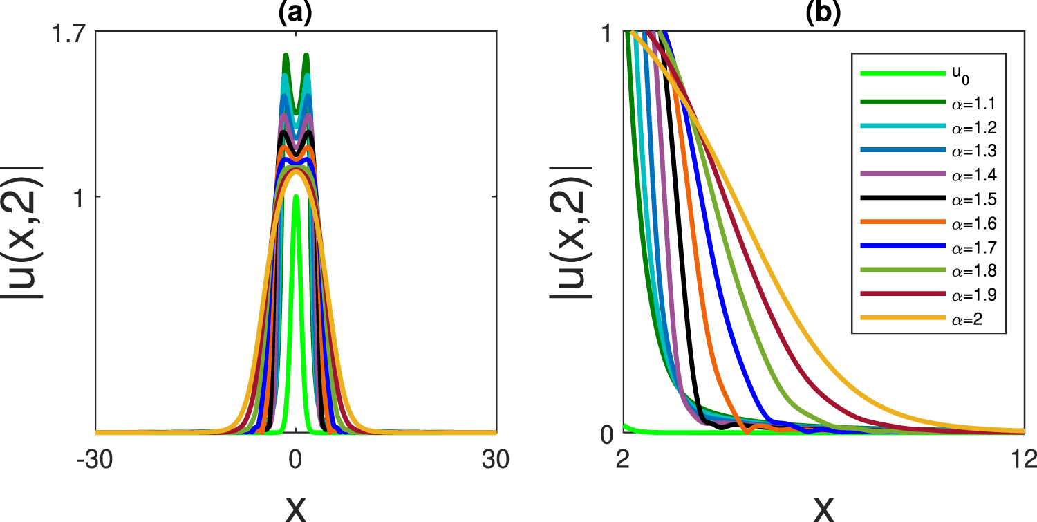
To compare the final intensity profiles of similaritons for varying $\alpha$ after the evolution of a standard unit Gaussian (with $x_0=1$) under the model equation (2), we plot the final intensity profiles (a) and their intermediate tails (b), superimposed, for a fixed gain $g=0.5$ at the propagation distance $z=2$ in Fig. 2.

At a short propagation distance ( $z=1$), the Gaussian evolves to a self-similar (similariton) profile for every $\alpha$, and these profiles becoming wider and lower in amplitude as $\alpha$ increases. As $\alpha$ approaches $2$ (the second-order-dispersion limit), the profile becomes more parabolic, whereas for smaller $\alpha$ it is more localized.

In Fig. 2, we further evolved the standard unit Gaussian until $z=2$ for varying $\alpha$ values to investigate the longer-distance behaviour of fractional similaritons. Here, we numerically observed two striking features of the previously obtained similaritons at $z=2$. Firstly, parabolic self-similar cores can be obtained only for $1.8 \leq \alpha \leq 2$. The rest of the profile-tops sink down to create two-peaked structures during the evolution and this phenomenon is even more pronounced for $1.1 \leq \alpha \leq 1.6$. Secondly, one can also observe a remarkable oscillatory behaviour in the intermediate tails for $1.5 \leq \alpha \leq 1.7$.

Figure 2.

(Colour online) (a) The final intensity profiles and (b) the tails of the intensity profiles at the propagation distance $z=2$, superimposed on the initial Gaussian pulse $u_0=e^{{-x}^2}$ for varying $\alpha$ and fixed gain $g=0.5$.

Figure 2 Long description

A line graph with the y-axis label, absolute value u left parenthesis x comma 2 right parenthesis and the x-axis label, x. The x-axis shows tick labels minus 30, 0 and 30. The y-axis shows tick labels 1 and 1.7. Multiple overlaid curves are centered at x equals 0. Each curve rises from near 0 at large negative x, forms a narrow peak around x equals 0 and returns to near 0 at large positive x. The tallest curve reaches just below the 1.7 tick. Several curves show a split top with two close maxima around x equals 0. The image B showing a line graph with the y-axis label, absolute value u left parenthesis x comma 2 right parenthesis and the x-axis label, x. The x-axis shows tick labels 2 and 12. The y-axis shows tick labels 0 and 1. A legend lists u subscript 0, alpha equals 1.1, alpha equals 1.2, alpha equals 1.3, alpha equals 1.4, alpha equals 1.5, alpha equals 1.6, alpha equals 1.7, alpha equals 1.8, alpha equals 1.9 and alpha equals 2. The u subscript 0 curve lies close to 0 across the plotted x-range. The alpha curves start near y equals 1 at x equals 2 and decrease toward y equals 0 as x increases. The alpha equals 1.1 curve drops to near 0 by about x equals 4. The alpha equals 1.2 curve drops to near 0 by about x equals 4.5. The alpha equals 1.3 curve drops to near 0 by about x equals 5. The alpha equals 1.4 curve drops to near 0 by about x equals 5.5. The alpha equals 1.5 curve drops to near 0 by about x equals 6. The alpha equals 1.6 curve drops to near 0 by about x equals 6.5. The alpha equals 1.7 curve drops to near 0 by about x equals 7. The alpha equals 1.8 curve drops to near 0 by about x equals 8. The alpha equals 1.9 curve drops to near 0 by about x equals 9. The alpha equals 2 curve decreases more gradually and approaches near 0 close to x equals 12.

In summary, as seen in Fig. 2, the profiles are parabolic for all $1.1 \leq \alpha \leq 2$ at the short distance $z=1$, whereas by $z=2$ two-peaked structures have formed and become more prominent for $1.1 \leq \alpha \leq 1.6$, a flat-top structure appears for $\alpha=1.7$ and $\alpha=1.8$ and parabolic tops are recovered for $\alpha=1.9$ and $\alpha=2$.

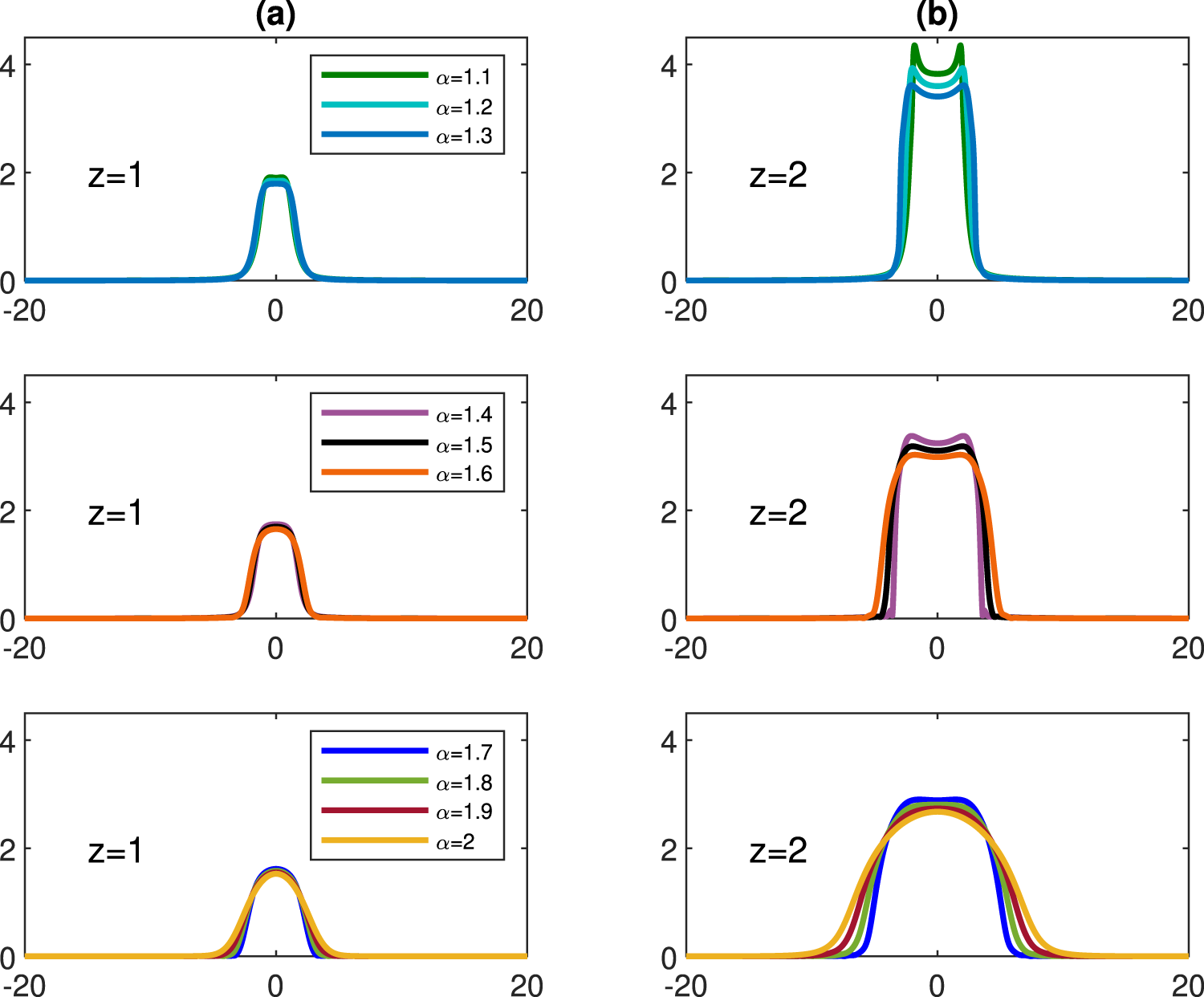
To observe the effect of gain in fractional similariton generation, we first evolved the standard Gaussian under increased gain, namely $g=1$. These results are shown in Fig. 3. One can observe from the final intensity profiles that are depicted on column (a) that the profiles corresponding to $1.1 \leq \alpha \leq 1.3$ are nearly flat-top structures and become more parabolic for $\alpha \geq 1.4$ for short-distance $z=1$ and in column (b), as $z$ increases up to 2, the two-peaked structures become more prominent for $1.1 \leq \alpha \leq 1.4$ and then for $1.5 \leq \alpha \leq 1.8$, the tops of the similariton structures become flatter and for $\alpha=1.9$ and for $\alpha=2$, the final intensity profiles become parabolic.

Figure 3.

(Colour online) Comparison of final intensity profiles at columns (a) $z=1$ and (b) $z=2$ for the initial Gaussian pulse $u_0=e^{{-x}^2}$ for varying $\alpha$, all with $g=1$.

Figure 3 Long description

Six line plots compare intensity profiles of Gaussian pulses for varying alpha values at two distances, z equals 1 and z equals 2. The horizontal axis represents an unlabeled coordinate and the vertical axis represents intensity, with no units provided. For z equals 1: - The first plot shows alpha values 1.1, 1.2 and 1.3, with nearly overlapping curves forming a narrow peak centered at 0, reaching a height near 2. - The second plot shows alpha values 1.4, 1.5 and 1.6, with curves forming a similar narrow peak, slightly broader than the first set. - The third plot shows alpha values 1.7, 1.8, 1.9 and 2, with curves forming a broader peak, indicating increased width with higher alpha. For z equals 2: - The first plot shows alpha values 1.1, 1.2 and 1.3, with curves forming a tall, flat-topped profile near 4, with a small central dip. - The second plot shows alpha values 1.4, 1.5 and 1.6, with a flat-topped profile around 3, slightly broader than the first set. - The third plot shows alpha values 1.7, 1.8, 1.9 and 2, with a broad profile peaking between 2 and 3, indicating further broadening. Alpha represents a parameter affecting the pulse shape and z represents the propagation distance. The plots illustrate how increasing alpha leads to broader and flatter intensity profiles, especially at greater distances.

Therefore, Figs 2 and 3 show that, as the unit Gaussian evolves under Eq. (2) for $z \gt rapprox 1$, for both gain values $g=0.5$ and $g=1$, the final intensity profiles become two-peaked structures if $\alpha \le 1.7 $. The emergence of these two-peaked cores is a direct manifestation of fractional dispersion. For the free (linear) equation, the group velocity associated with wavenumber $k$ is $v(k)=(\beta/2)\alpha|k|^{\alpha-1}\mathrm{sgn}(k)$, which – unlike the single-valued law $v=\beta k$ of the classical case $\alpha=2$ – collapses onto the two constant values $v=\pm\beta/2$ as $\alpha\to1$, so that a localized input tends to break into two lobes that separate linearly with distance. Equivalently, the fractional free-propagation kernel is two-peaked for $\alpha \lt 2$, and propagation convolves the input into two beams, the one-dimensional analogue of the conical diffraction reported by Zhang et al. [Reference Zhang, Liu, Belić, Zhong, Zhang and Xiao34, Reference Zhang, Zhong, Belić, Ahmed, Zhang and Xiao35]. The same splitting, and its group-velocity origin, was recently analysed for the semiclassical fractional Schrödinger equation by Klein and Sparber [Reference Klein and Sparber17], whose group velocity $v(\xi)=2s\,\mathrm{sgn}(\xi)|\xi|^{2s-1}$ (with $s=\alpha/2$) coincides with the expression above. This is shown in Fig. 4 for the linear equation: a Gaussian remains single-peaked at $\alpha=2$ but splits into two separating lobes for $\alpha \lt 2$, the more rapidly the smaller $\alpha$ is. In the present non-linear, amplified setting the Kerr self-phase modulation broadens the spectrum and populates the higher- $|k|$ components that carry the larger splitting velocities, accelerating the splitting so that the two-peaked core already appears at the moderate distances $z\simeq2$– $4$ studied here. As $\alpha$ increases, the pulse passes from the strongly split two-peaked regime, through an intermediate flat-top crossover, to the single-peaked parabolic profile recovered at $\alpha=2$, the central depression decreasing monotonically throughout.

Figure 4.

(Colour online) Fractional beam splitting in the linear equation (no non-linearity, no gain): $|u(x,z)|$ for an initial Gaussian. (a) At $\alpha=2$, the beam spreads while remaining single-peaked; (b), (c) for $\alpha \lt 2$, it splits into two lobes that separate linearly with $z$, the more rapidly the smaller $\alpha$ is. This linear splitting, accelerated by the Kerr non-linearity, underlies the two-peaked cores.

Figure 4 Long description

Three 3D surface plots illustrate the behavior of |u| over the axes labeled X and Z for varying alpha values. In the first plot, labeled (a) with alpha equals 2, the surface shows a single peak centered around X equals 0 and Z equals 5. The second plot, labeled (b) with alpha equals 1.5, displays a split into two peaks, with the peaks diverging as Z increases. The third plot, labeled (c) with alpha equals 1.1, shows a more pronounced separation of the peaks, with the peaks moving further apart as Z increases. The X-axis ranges from -20 to 20 and the Z-axis ranges from 0 to 10 in all plots. The vertical axis represents |u|, ranging from 0 to 1.

To observe the longer-distance evolution of the fractional similaritons, we first depicted the evolution of the fractional similariton for $\alpha=1.5$ for a long distance ( $z=4$) that is shown in Fig. 5 for $g=0.5$ in (a) and for $g=1$ in (b). Although the intensity profiles are quite similar for $z=2$ for both cases (see Figs 2 and 3), it is seen from the figure that, as the Gaussian initial conditions are further evolved up to $z=4$, higher gain supports a more parabolic profile, and on the other hand, lower gain supports a two-peaked profile, which becomes nearly flat-top around the last steps of the evolution.

Figure 5.

(Colour online) Evolution of a similariton: propagation distance $z=4$ for $\alpha=1.5$ for the initial Gaussian pulse $u_0=e^{-{x}^2}$ in (a) $g=0.5$ and in (b) $g=1$.

Figure 5 Long description

A showing a three dimensional line surface plot. The vertical axis label is magnitude of u, with tick labels 0, 1 and 2. The axis labeled x has tick labels minus 20, 0 and 20. The axis labeled z has tick labels 0, 2 and 4. Multiple stacked curves run along x at increasing z values from 0 to 4. At z equals 0, the curve is near 0 across x. As z increases, a narrow central peak forms near x equals 0 and increases in height. By z equals 4, the peak rises above the tick label 2, while values away from the center remain close to 0. B showing a three dimensional line surface plot. The vertical axis label is magnitude of u, with tick labels 0, 5, 10 and 15. The axis labeled x has tick labels minus 20, 0 and 20. The axis labeled z has tick labels 0, 2 and 4. Multiple stacked curves run along x at increasing z values from 0 to 4. At z equals 0, the curve is near 0 across x. As z increases, a central peak forms near x equals 0 and increases in height. By z equals 4, the peak rises above the tick label 15, while values away from the center remain close to 0.

This result raises the question about the effect of gain and evolution distance on the fractional similaritons. For what values of $\alpha$ does an increase in gain produce a threshold in the existence of similaritons for longer evolution distances (in this study, we only assume $z=4$)?

We have numerically investigated the effect of increasing gain and evolution distance on the fractional similaritons that are obtained with the standard Gaussian initial condition. To demonstrate this, we have fixed the evolution distance to $z=4$ and observed the evolution for various values of gain, namely for $g=0$ (no gain), $g=0.1, 0.3, 0.5$ and $g=1$.

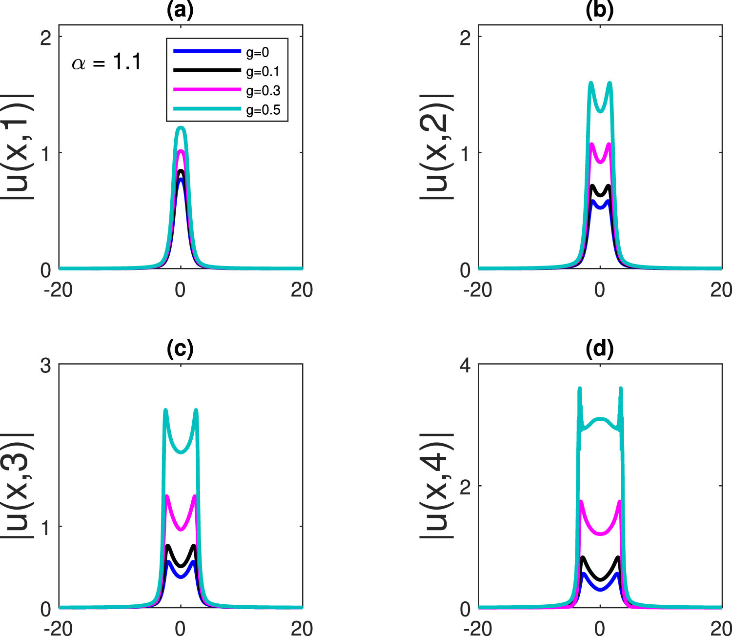
Our numerical simulations show that, for $z=4$, fractional similaritons are supported only for relatively small gain values ( $0 \leq g \leq 0.5$) when $\alpha$ is small ( $1.1 \leq \alpha \leq 1.4$). However, beyond $z=1$, the evolving pulse develops a two-peaked intensity profile, indicating a deviation from self-similar evolution. As the gain is increased to $g=1$, these similariton-like structures completely deteriorate during propagation. Therefore, for smaller values of $\alpha$, the gain is limited to $g \leq 0.5$ to maintain stable evolution.

Unlike the case for smaller $\alpha$, for $\alpha \geq 1.5$, larger gain values (up to $g=1$ in the present study) lead to increasingly parabolic intensity profiles, whereas smaller gain values produce flat-top similaritons. These results are illustrated in Fig. 6 for $\alpha=1.1$, where the effect of increasing gain on the pulse evolution is demonstrated (cf. Fig. 5 for $\alpha=1.5$).

For $\alpha \geq 1.6$, the final intensity profiles become increasingly parabolic, as expected, indicating that the propagation is self-similar only for these larger values of $\alpha$. This behaviour is anticipated because, as $\alpha$ approaches 2, the fractional dispersion operator increasingly resembles the standard second-order dispersion term, $u_{xx}$. Consequently, the dynamics gradually recover the conventional self-similar evolution characteristic of the classical dispersion regime. The suppression of the two-peaked core by gain has a simple interpretation. In a normal-dispersion amplifier, the parabolic self-similar pulse is an asymptotic attractor [Reference Fermann, Kruglov, Thomsen, Dudley and Harvey10, Reference Kruglov, Peacock and Harvey18], and gain drives the field towards this single-peaked state, competing with the fractional splitting. Without gain, there is no such attractor and the central depression only deepens with distance; with gain it instead fills in, the more rapidly the larger the gain, since the self-similar scale grows as $e^{2gz/3}$ and a larger gain carries the pulse through more gain lengths $\sim g^{-1}$ over a fixed distance. This same competition explains the upper gain limit found for small $\alpha$: when $\alpha\lesssim1.4$, the fractional dispersion is too weak to sustain a stable attractor against rapid amplification, so at $g=1$ the structure fragments rather than converging, which is why stable evolution for small $\alpha$ is confined to $g\lesssim0.5$.

Figure 6.

(Colour online) The final intensity profiles at the propagation distances (a) $z=1$, (b) $z=2$, (c) $z=3$ and (d) $z=4$ for varying gains all with $\alpha=1.1$ and initial Gaussian pulse $u_0=e^{{-x}^2}$.

Figure 6 Long description

A line plot labeled alpha equals 1.1 with a legend listing g equals 0, g equals 0.1, g equals 0.3 and g equals 0.5. The x-axis is unlabeled, ranging from minus 20 to 20 with labeled ticks at minus 20, 0 and 20. The y-axis label is absolute u open parenthesis x comma 1 close parenthesis, ranging from 0 to 2 with labeled ticks at 0, 1 and 2. All four curves are near 0 for most x values and form a narrow peak centered at x equals 0. The peak height increases with g, with the tallest curve reaching a little above 1 and the smallest peak below 1. The image B showing a line plot with the x-axis unlabeled, ranging from minus 20 to 20 with labeled ticks at minus 20, 0 and 20. The y-axis label is absolute u open parenthesis x comma 2 close parenthesis, ranging from 0 to 2 with labeled ticks at 0, 1 and 2. Four curves are overlaid and concentrated near x equals 0. Each curve forms a narrow central feature with a split top, creating two close peaks around x equals 0. The highest curve rises to between 1 and 2, while the lowest curve rises to below 1. The image C showing a line plot with the x-axis unlabeled, ranging from minus 20 to 20 with labeled ticks at minus 20, 0 and 20. The y-axis label is absolute u open parenthesis x comma 3 close parenthesis, ranging from 0 to 3 with labeled ticks at 0, 1 and 3. Four curves are overlaid and confined near x equals 0. The curves form a narrow structure with a central dip and two higher sides near the top, producing a double peaked shape. The tallest curve rises to between 2 and 3 and the smallest curve rises to below 1. The image D showing a line plot with the x-axis unlabeled, ranging from minus 20 to 20 with labeled ticks at minus 20, 0 and 20. The y-axis label is absolute u open parenthesis x comma 4 close parenthesis, ranging from 0 to 4 with labeled ticks at 0, 2 and 4. Four curves are overlaid and concentrated near x equals 0. The curves form a broad, flat topped region with steep sides and the highest curve shows two narrow spikes near the left and right edges of the flat top. The tallest curve rises to between 3 and 4, while the lowest curve rises to below 1.

4. Effect of the initial condition on the self-similar evolution

In this section, we investigate the influence of the initial pulse on the self-similar evolution of fractional similaritons. As demonstrated in the previous section, a standard Gaussian initial pulse may evolve into a two-peaked, flat-top or parabolic similariton, depending on the fractional order $\alpha$, the gain $g$ and the propagation distance $z$. While flat-top profiles may be desirable for certain applications, the two-peaked structures are generally less robust during propagation, whereas parabolic profiles are expected to exhibit superior stability.

Furthermore, the obtained pulse profiles exhibit similar shapes and propagation dynamics within groups of nearby $\alpha$ values. For a more meaningful comparison across the entire range of $\alpha$, it is desirable to obtain a parabolic-like intensity profile for each fractional order by appropriately tailoring the initial condition.

Here, we demonstrate that this issue can be resolved by employing a stretched Gaussian initial pulse with a stretching factor $x_0$, namely, $u_0=e^{-{(x/x_0)}^2}$.

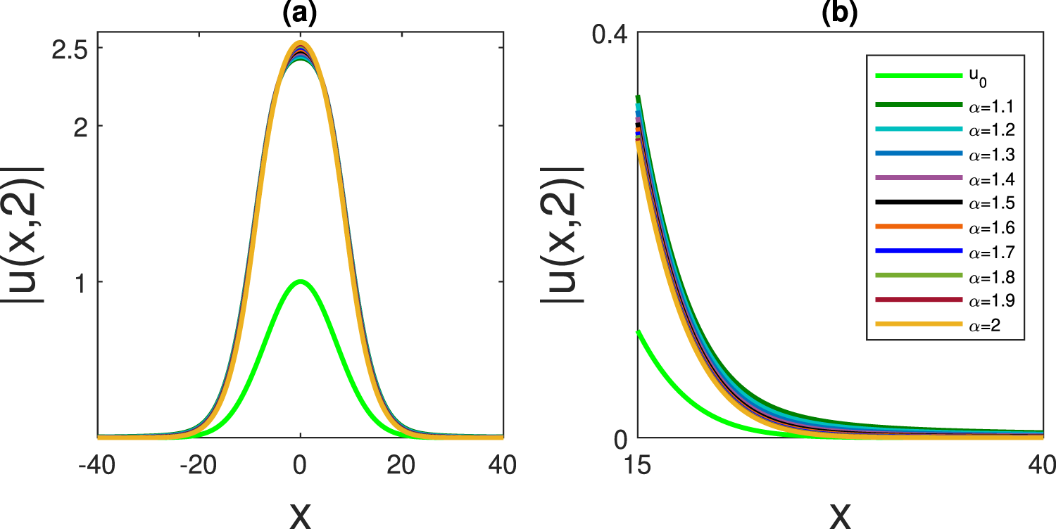
A remarkable result is presented in Fig. 7. By employing a stretched Gaussian initial pulse with $x_0=10$, a self-similar intensity profile is obtained across the entire range of $\alpha$ considered in this study, for a fixed gain of $g=0.5$ and the propagation distance of $z=2$.

Compared with Fig. 2, the stretched Gaussian initial pulse effectively eliminates the collapse of the core region observed for $1.1 \leq \alpha \leq 1.7$. That a wider input suppresses the splitting is likewise a propagation effect. The splitting requires a finite distance to develop, set by the dispersion length $L_D\sim W^{\alpha}/|\beta|$ of a pulse of width $W$: a narrow input ( $W\sim1$) has $L_D\lesssim z$ and splits within the propagation distance, whereas a stretched input has $L_D\gg z$ and barely evolves, so that the gain simply amplifies it onto the parabola. We emphasize that this is a width effect rather than an energy effect – the stretched and unstretched Gaussians share the same peak power – and it is governed by $L_D$ alone; because $L_D\sim x_0^{\alpha}$ exceeds the propagation distance once $x_0$ is sufficiently large, the stretched input yields a clean parabolic profile across the entire range of $\alpha$.

It is also evident from Fig. 7 that, although the peak amplitudes of the self-similar profiles increase with $\alpha$, their maximum values remain confined to a narrow range around $\lvert u \rvert=2.5$. In addition, the oscillatory structures previously appearing in the intermediate tails for $1.4 \leq \alpha \leq 1.7$ are completely suppressed.

Figure 7.

(Colour online) (a) The final intensity profiles and (b) the intermediate tails at the propagation distance $z=2$ for the initial Gaussian pulse $u_0=e^{-{(x/10)}^2}$ for varying $\alpha$ and fixed gain $g=0.5$.

Figure 7 Long description

The line graph with the y-axis labeled, absolute value of u left parenthesis x comma 2 right parenthesis and the x-axis labeled, x. The x-axis shows tick labels at minus 40, minus 20, 0, 20 and 40. The y-axis shows tick labels at 1, 2 and 2.5. Multiple smooth curves form a symmetric peak centered at x equals 0. One thicker curve peaks near y equals 1 at x equals 0 and decreases toward y near 0 by about x equals minus 20 and x equals 20. The remaining curves overlap closely, peaking slightly above y equals 2.5 at x equals 0 and decreasing toward y near 0 by about x equals minus 20 and x equals 20. The line graph with the y-axis labeled, absolute value of u left parenthesis x comma 2 right parenthesis and the x-axis labeled, x. The x-axis shows tick labels at 15 and 40. The y-axis shows tick labels at 0 and 0.4. A legend lists, u subscript 0, alpha equals 1.1, alpha equals 1.2, alpha equals 1.3, alpha equals 1.4, alpha equals 1.5, alpha equals 1.6, alpha equals 1.7, alpha equals 1.8, alpha equals 1.9 and alpha equals 2. All curves decrease from left to right. The u subscript 0 curve starts near y equals 0.1 at x equals 15 and approaches y near 0 by x equals 40. The alpha curves start between about y equals 0.3 and y equals 0.35 at x equals 15 and approach y near 0 by x equals 40, with the curves closely grouped throughout the range.

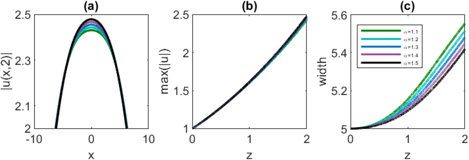
To further analyse the results shown in Fig. 7, Fig. 9(a)–(c) displays the core region of the final intensity profiles, as well as the evolution of the peak amplitude and the width of the self-similar profiles with propagation distance $z$, for the representative range $1.1 \leq \alpha \leq 1.5$; the behaviour for $1.6 \leq \alpha \leq 2$ is analogous.

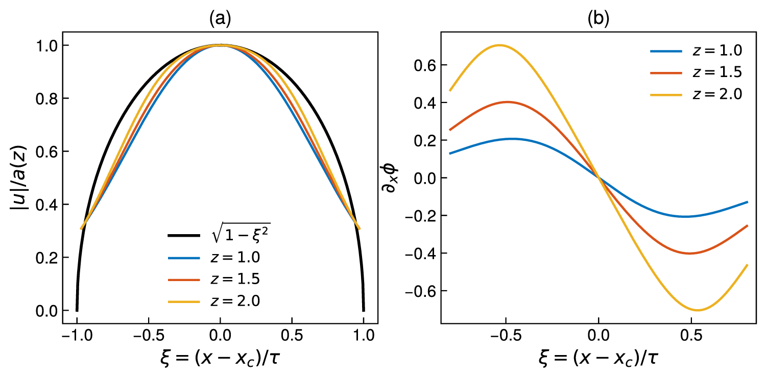
In these plots, the core regions of the final intensity profiles reveal that, by employing a stretched Gaussian initial condition, a self-similar parabolic profile is consistently obtained. Moreover, the monotonic evolution of the peak amplitude and the profile width confirms that the pulse evolves towards a similariton in each case. To place the term similariton on a quantitative footing, Fig. 8(a) rescales the parabolic profiles at successive distances by their amplitude $a(z)$ and width $\tau(z)$: the rescaled profiles collapse onto the universal parabola $\sqrt{1-\xi^2}$, the RMS deviation from this shape decreasing with propagation (from $10\%$ at $z=1$ to $6\%$ at $z=2$), which confirms genuine self-similar evolution; these parabolic states persist over the full propagation range studied, growing self-similarly without degradation. The corresponding instantaneous chirp $\partial_x\phi$ is linear at each propagation distance (Fig. 8(b)), as required of a parabolic similariton, the chirp rate increasing during propagation. We stress that only these single-peaked parabolic profiles are genuine, self-similar similaritons; the two-peaked structures of Section 3 are not self-similar states but the transient signature of the fractional splitting being suppressed by the gain, and they relax towards the parabolic similariton as the distance and gain increase.

Figure 8.

(Colour online) Quantitative self-similarity of the parabolic similariton (stretched input, $\alpha=1.5$, $g=0.5$). (a) Profiles at $z=1,1.5,2$, rescaled by the amplitude $a(z)$ and width $\tau(z)$, collapse onto the universal parabola $\sqrt{1-\xi^2}$, $\xi=(x-x_c)/\tau$. (b) The corresponding instantaneous chirp $\partial_x\phi$ is linear at each distance $z=1,1.5,2$, confirming the linear chirp of a parabolic similariton.

Figure 8 Long description

A showing a multi-line graph of vertical bars u vertical bars slash a left parenthesis z right parenthesis versus xi equals left parenthesis x minus x subscript c right parenthesis slash tau. The legend lists, square root of 1 minus xi squared, z equals 1.0, z equals 1.5 and z equals 2.0. The horizontal axis range is negative 1.0 to 1.0. The vertical axis range is 0.0 to 1.0. All plotted curves form a single symmetric arch centered at xi equals 0.0, with the highest point near vertical bars u vertical bars slash a left parenthesis z right parenthesis equals 1.0 at xi equals 0.0. The reference curve labeled square root of 1 minus xi squared forms the outer boundary of the arch. The three z curves lie inside the reference curve for most xi values and approach the reference curve near xi values close to negative 1.0 and 1.0. The z equals 1.0, z equals 1.5 and z equals 2.0 curves are closely spaced near the peak and separate more toward the sides, with the z equals 2.0 curve appearing slightly narrower around the center than the z equals 1.0 curve. B showing a multi-line graph of partial subscript x phi versus xi equals left parenthesis x minus x subscript c right parenthesis slash tau. The legend lists, z equals 1.0, z equals 1.5 and z equals 2.0. The horizontal axis range is negative 0.8 to 0.8. The vertical axis range is negative 0.6 to 0.6. Each curve crosses the horizontal axis at xi equals 0.0. For negative xi values, each curve is above 0.0 and forms a single positive lobe. For positive xi values, each curve is below 0.0 and forms a single negative lobe. The magnitude of the lobes increases with z: the z equals 1.0 curve has the smallest positive and negative excursions, the z equals 1.5 curve is larger and the z equals 2.0 curve is largest. The positive lobe peaks around xi near negative 0.5 and the negative lobe reaches its lowest point around xi near 0.5 for all three curves. No plotted coordinate pairs are readable with sufficient certainty from the curves.

Figure 9.

(Colour online) (a) Core region of the intensity profile at the final distance $z=2$, (b) evolution distance $z$ versus the maximum amplitude and (c) evolution distance $z$ versus the width of the self-similar profiles for $1.1 \leq \alpha \leq 1.5$ for the initial Gaussian pulse $u_0=e^{-{(x/10)}^2}$ and $g=0.5$.

Figure 9 Long description

A line graph with the horizontal axis labeled, x, ranging from negative 10 to 10 and the vertical axis labeled, vertical bar u left parenthesis x comma 2 right parenthesis vertical bar, ranging from 2.0 to 2.5. Several smooth curves form an inverted arch shape, with the highest values near x equals 0 and lower values toward x equals negative 10 and x equals 10. The image B showing a line graph with the horizontal axis labeled, z, ranging from 0 to 2 and the vertical axis labeled, max left parenthesis u right parenthesis, ranging from 1.0 to 2.5. Several curves rise from near 1.0 at z equals 0 to near 2.5 at z equals 2. The image C showing a line graph with the horizontal axis labeled, z, ranging from 0 to 2 and the vertical axis labeled, width, ranging from 5.0 to 5.6. Several curves increase from near 5.0 at z equals 0 to values between about 5.4 and 5.6 at z equals 2. A legend lists multiple series labels.

Figure 10 presents a comparison between the similaritons generated from (a) a standard Gaussian input and (b) a stretched Gaussian input after propagation to $z=2$, with $\alpha=1.3$ and $g=0.5$ in both cases. It is evident that the stretched Gaussian input gives rise to a smooth parabolic self-similar profile, whereas the standard Gaussian input evolves into a more localized two-peaked similariton.

Figure 10.

(Colour online) Evolution of a similariton: for the initial Gaussian pulse (a) $u_0=e^{-{x}^2}$ and (b) $u_0=e^{-{(x/10)}^2}$, both with $g=0.5$, propagation distance $z=2$ and for $\alpha=1.3$.

Figure 10 Long description

A 3D line plot labeled, a. The x-axis is labeled, x, with tick labels at minus 20, 0 and 20. The z-axis is labeled, z, with tick labels at 0, 1 and 2. The vertical axis is labeled, magnitude of u, with tick labels at 0, 0.5, 1.0 and 1.5. Units are not indicated for x, z, or magnitude of u. A set of multiple line traces is plotted at successive z values from 0 to 2. Across the traces, the profile stays near 0 for most x values and forms a narrow peak centered near x equals 0. The peak height increases with z, reaching about 1.5 near z equals 2. A 3D line plot labeled, b. The x-axis is labeled, x, with tick labels at minus 20, 0 and 20. The z-axis is labeled, z, with tick labels at 0, 1 and 2. The vertical axis is labeled, magnitude of u, with tick labels at 0, 1, 2 and 3. Units are not indicated for x, z, or magnitude of u. A set of multiple line traces is plotted at successive z values from 0 to 2. Across the traces, the profile forms a single broad peak centered near x equals 0, with values decreasing toward x equals minus 20 and x equals 20. The peak height increases with z, reaching about 3 near z equals 2.

To analyse the influence of the initial condition for longer evolution distances (in this study, we took $z=4$), we evolved three different initial inputs ( $u_0=e^{-{x}^2}$, $u_0=e^{-{(x/5)}^2}$ and $u_0=e^{-{(x/10)}^2}$) for increasing gain, namely, $g=0.1, 0.3, 0.5$ and $g=1$ for various values of the fractional order $\alpha$.

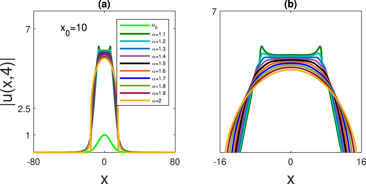
Our numerical simulations show that, for the most stretched initial input $u_0=e^{-{(x/10)}^2}$:

1. (i) For $g=0.3$: The final intensity profiles are two-peaked (due to collapse of the core) for $1.1 \leq \alpha \leq 1.4$, flat-top for $1.5 \leq \alpha \leq 1.7$ and become parabolic for $1.8 \leq \alpha \leq 2$.

2. (ii) For $g=0.5$: The final intensity profiles are two-peaked (peaks are even more pronounced when compared to $g=0.3$ case) for $1.1$ and $1.2$, flat-top for $1.3$, $1.4$ and $1.5$ and then become parabolic for $1.6 \leq \alpha \leq 2$. We present these results in Fig. 11.

Figure 11.

(Colour online) (a) The final intensity profiles. (b) Core region of the intensity profile at the final distance $z=4$, all for $g=0.5$, $u_0=e^{-{(x/10)}^2}$.

Figure 11 Long description

A line graph with the text, x subscript 0 equals 10. The x-axis label is x, with tick labels at minus 80, 0 and 80. The y-axis label is vertical bar u left parenthesis x comma 4 right parenthesis vertical bar, with tick labels at 1, 2.5 and 7. A legend lists u subscript 0, alpha equals 1.1, alpha equals 1.2, alpha equals 1.3, alpha equals 1.4, alpha equals 1.5, alpha equals 1.6, alpha equals 1.7, alpha equals 1.8, alpha equals 1.9 and alpha equals 2. One curve labeled u subscript 0 forms a low, rounded peak centered near x equals 0, reaching about y equals 1. The alpha curves form a tall, narrow central region centered near x equals 0 with steep sides. Near the top of this region, several curves show two small local maxima separated by a shallow dip. The curves approach y near 0 toward x near minus 80 and x near 80. The image B showing a line graph. The x-axis label is x, with tick labels at minus 16, 0 and 16. The y-axis has a tick label at 7. Multiple curves form a broad, flat central top around x equals 0, with the top height varying by curve. Several curves show small peaks near the left and right edges of the flat region before dropping downward. The curves descend toward the lower part of the plot as x approaches minus 16 and 16.

We observe numerically that, for stretched Gaussian inputs, the intensity profiles deteriorate during propagation when the gain is increased to $g=1$. Consequently, only the results corresponding to lower gain values are presented below.

To illustrate the influence of the initial pulse width, Fig. 12 shows the evolution of three Gaussian initial inputs with different widths, $ u_0=e^{-x^2}, \quad u_0=e^{-(x/5)^2}, \quad u_0=e^{-(x/10)^2}$ for a fixed fractional order ( $\alpha=1.1$). Panels (a), (b) and (c) correspond to these three inputs, all at a fixed gain $g=0.5$. The figure clearly demonstrates that increasing the width of the initial Gaussian pulse leads to the formation of a broader and less localized similariton.

Figure 12.

(Colour online) Evolution of a similariton: for the initial Gaussian pulse in (a) $u_0=e^{-{x}^2}$, (b) $u_0=e^{-{(x/5)}^2}$ and (c) $u_0=e^{-{(x/10)}^2}$ all with $g=0.5$, propagation distance $z=4$ and for $\alpha=1.1$.

Figure 12 Long description

The plots illustrate the evolution of a similariton for different initial Gaussian pulse widths. All panels share the same axes: x-axis labeled x, ranging from minus 20 to 20; z-axis labeled z, ranging from 0 to 4; and the vertical axis labeled magnitude u. In panel (a), the plot shows a narrow ridge near x equals 0, rising sharply in magnitude u as z increases, peaking around 4. Panel (b) displays a similar ridge, slightly broader than in (a), with magnitude u peaking around 5. Panel (c) shows the broadest ridge, with magnitude u peaking around 5.5. The plots demonstrate how increasing the initial pulse width results in a broader and less localized similariton.

Figure 13.

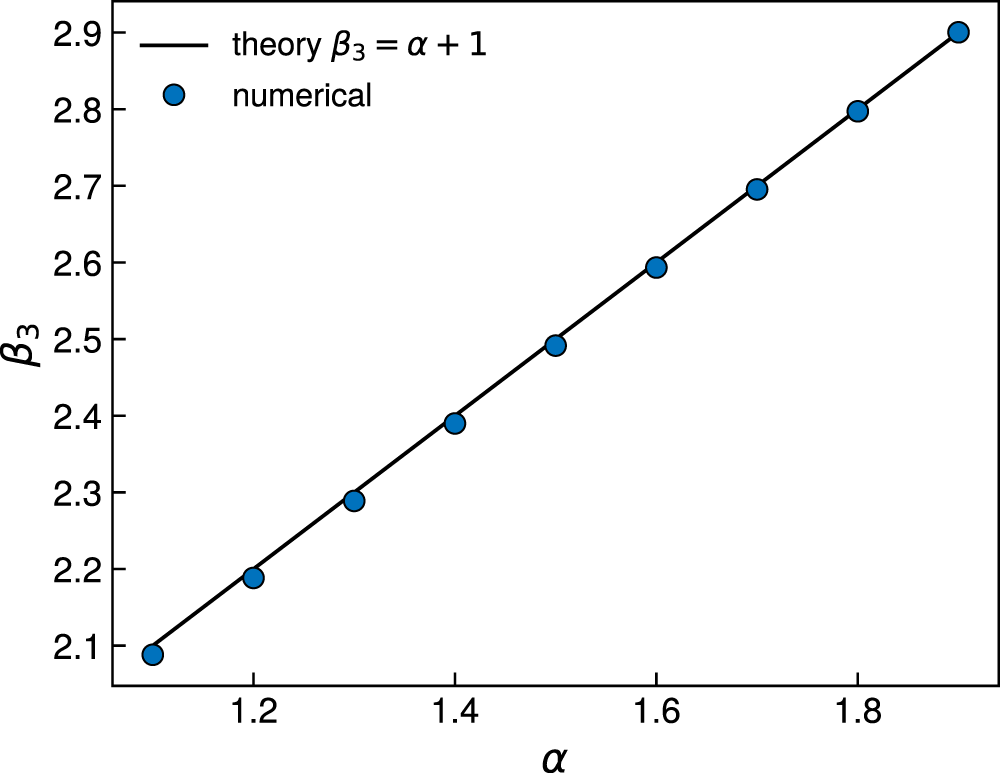
(Colour online) Far-tail decay exponent $\beta_3$ extracted from the numerical solutions at $z=2$ (symbols), compared with the theoretical prediction $\beta_3=\alpha+1$ (line).

For the fractional order $\alpha=1.5$, a flat-top core emerges even at the relatively small gain value $g=0.3$.

5. Tail analysis of fractional similaritons

A remarkable consequence of fractional dispersion is the emergence of heavy-tailed waveforms, which fundamentally distinguishes fractional similaritons from their classical counterparts. In the standard NLS equation $(\alpha=2)$, optical pulses remain strongly localized owing to the exponential decay of their tails. However, when the second-order dispersion operator is replaced by the fractional derivative, the propagation dynamics become non-local, resulting in algebraically decaying pulse wings. Consequently, a considerable portion of the optical energy is transported away from the pulse centre, producing long-range tails that are characteristic of Lévy-type wave propagation.

Before investigating the heavy-tail characteristics of fractional similaritons, it is essential to establish the propagation behaviour of the classical NLS equation corresponding to the integer-order dispersion ( $\alpha = 2$).

(9)\begin{equation} |u(x)| \sim A \exp(-\beta_1 |x|), \quad |u(x)| \sim B\exp(-\beta_2 |x|^2) \end{equation}

where $A$ and $B$ represent the amplitude coefficient and $\beta_{1,2}$ is the exponential decay constant. This exponential localization is a characteristic feature of solutions governed by the classical NLS equation. Unlike the classical NLS equation, where exponentially localized solutions are obtained, the fractional derivative generates algebraically decaying solutions. Therefore, the localized stationary solution exhibits the asymptotic behaviour

(10)\begin{equation} u(x,z)\sim C |x|^{-\beta_3}, \qquad |x|\rightarrow\infty \end{equation}

where $C$ represents the amplitude coefficient and $\beta_3$ is the power-law decay constant. Equation (10) demonstrates that fractional similaritons possess algebraically decaying heavy tails. Theoretically, the tails can also be approximated by a power-law function of the form $u(x,z) \sim a |x|^{-(\alpha+1)}$, so that $\beta_3 = \alpha+1$; this exponent agrees with the rigorous decay theory for fractional Schrödinger ground states [Reference Secchi30] and with recent numerical studies of fractional NLS solitons and $\phi^4$ kinks [Reference Decker, Demirkaya, Alexander and Kevrekidis7, Reference Decker, Demirkaya, Alexander, Tsolias and Kevrekidis8], which report the same $|x|^{-(\alpha+1)}$ far-tail law. This exponent is confirmed quantitatively in Fig. 13, which compares the decay exponent extracted from the numerically computed tails at $z=2$ with the theoretical value $\alpha+1$ across the full range of $\alpha$; the agreement is excellent, to within $\pm0.02$. The tail decays more slowly the smaller $\alpha$ is, so that a growing fraction of the optical power is carried into the wings – the Lévy-type, rather than Gaussian, transport characteristic of fractional media [Reference Longhi24, Reference Malomed25]. As $\alpha\to2$, the coefficient of the algebraic tail collapses and the exponential localization of the classical NLS is recovered, reconciling the exponential decay obtained at $\alpha=2$ with the algebraic decay found for every $\alpha \lt 2$.

Figure 14.

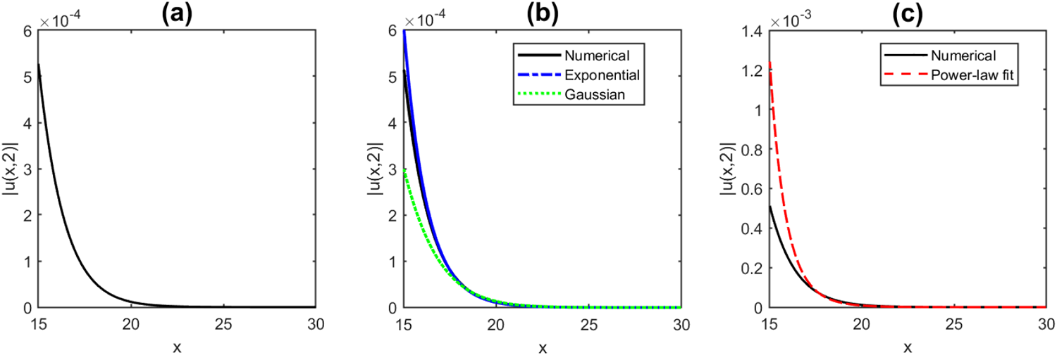
Numerical profile and asymptotic tail analysis of the similariton at the propagation distance $z=2$. (a) Numerical profile $\vert u(x,2)\vert$, (b) comparison of the numerical tail with the exponential and Gaussian decay models in the tail region $(15 \lt x \lt 30)$ and (c) comparison of the numerical tail with power-law model in the tail region $(15 \lt x \lt 30)$.

Figure 14 Long description

Line graphs labeled A, B and C. A shows a line graph with the horizontal axis labeled x and the vertical axis labeled u. The horizontal axis ranges from 15 to 30. The vertical axis ranges from 0 to 6 times 10 superscript negative 4. A single curve decreases from about 6 times 10 superscript negative 4 near x equals 15 toward 0 by about x equals 30. B shows a line graph with the horizontal axis labeled x and the vertical axis labeled u. The horizontal axis ranges from 15 to 30. The vertical axis ranges from 0 to 6 times 10 superscript negative 4. A legend lists Numerical, Exponential and Gaussian. Three curves decrease from about 6 times 10 superscript negative 4 near x equals 15 toward 0 by about x equals 30. C shows a line graph with the horizontal axis labeled x and the vertical axis labeled u. The horizontal axis ranges from 15 to 30. The vertical axis ranges from 0 to 1.4 times 10 superscript negative 4. A legend lists Numerical and Power law. Two curves decrease from about 1.3 times 10 superscript negative 4 near x equals 15 toward 0 by about x equals 30.

Figure 15.

Near and far tails of similaritons for different fractional orders $\alpha$ at fixed gain $g=0.5$ and propagation distance $z=2$.

Figure 15 Long description

The line graph A has three curves and one inset. The x-axis is labeled, x, with tick labels 5, 10, 15, 20. The y-axis is labeled, vertical bar u open parenthesis x comma 2 close parenthesis vertical bar, with tick labels 0, 0.1, 0.2, 0.3, 0.4, 0.5. A legend lists alpha equals 1.1, alpha equals 1.3, alpha equals 1.4. The three curves start near y equals 0.5 at x near 0 and drop steeply toward y equals 0 by about x between 4 and 6, then remain near 0 through x equals 20. The inset has x-axis tick labels 40, 60, 80 and y-axis tick labels 0 and 1, with the text, times 10 superscript minus 3, printed near the inset. In the inset, three curves decrease from near y equals 1 at x near 30 to near y equals 0 by x equals 80. The line graph B has three curves and one inset. The x-axis is labeled, x, with tick labels 5, 10, 15, 20. The y-axis is labeled, vertical bar u open parenthesis x comma 2 close parenthesis vertical bar, with tick labels 0, 0.5, 1, 1.5. A legend lists alpha equals 1.5, alpha equals 1.6, alpha equals 1.8. The three curves start near y between 1.0 and 1.5 at x near 0 and drop steeply toward y equals 0 by about x between 4 and 6, then remain near 0 through x equals 20. The inset has x-axis tick labels 40, 60, 80 and y-axis tick labels 0 and 1, with the text, 5 times 10 superscript minus 4, printed near the inset. In the inset, three curves decrease from near y equals 1 at x near 30 to near y equals 0 by x equals 80.

Figure 16.

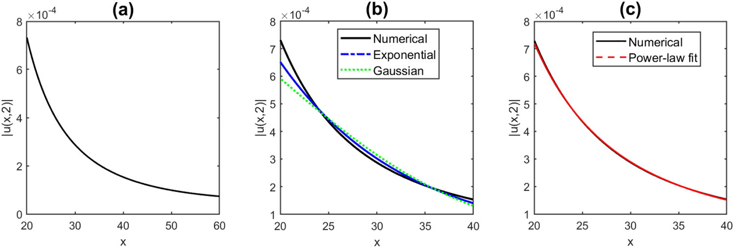
Numerical profile and asymptotic tail analysis of the similariton at the propagation distance $z=2$ for $\alpha=1.4$. (a) Numerical profile $\vert u(x,2)\vert$, (b) comparison of the numerical tail with the exponential and Gaussian decay models in the tail region $(20 \lt x \lt 60)$ and (c) comparison of the numerical tail with power-law model in the tail region $(20 \lt x \lt 60)$.

Figure 16 Long description

The line graph A shows psi x versus x. The x-axis label is, x, with tick labels 20, 30, 40, 50, 60. The y-axis label is, psi x, with tick labels 0, 2, 4, 6, 8 and a multiplier text, times 10 superscript minus 4. One curve decreases smoothly from about 8 times 10 superscript minus 4 at x equals 20 toward 0 by x equals 60. The line graph B shows psi x versus x with three overlaid curves. The x-axis label is, x, with tick labels 20, 25, 30, 35, 40. The y-axis label is, psi x, with tick labels 0, 2, 4, 6, 8 and a multiplier text, times 10 superscript minus 4. The legend lists, Numerical, Exponential, Gaussian. All three curves start near 8 times 10 superscript minus 4 at x equals 20 and decrease toward about 0 by x equals 40. The three curves remain closely spaced across the plotted x range. The line graph C shows psi x versus x with two overlaid curves. The x-axis label is, x, with tick labels 20, 25, 30, 35, 40. The y-axis label is, psi x, with tick labels 0, 2, 4, 6, 8 and a multiplier text, times 10 superscript minus 4. The legend lists, Numerical, Power law fit. Both curves start near 8 times 10 superscript minus 4 at x equals 20 and decrease toward about 0 by x equals 40.

Figure 17.

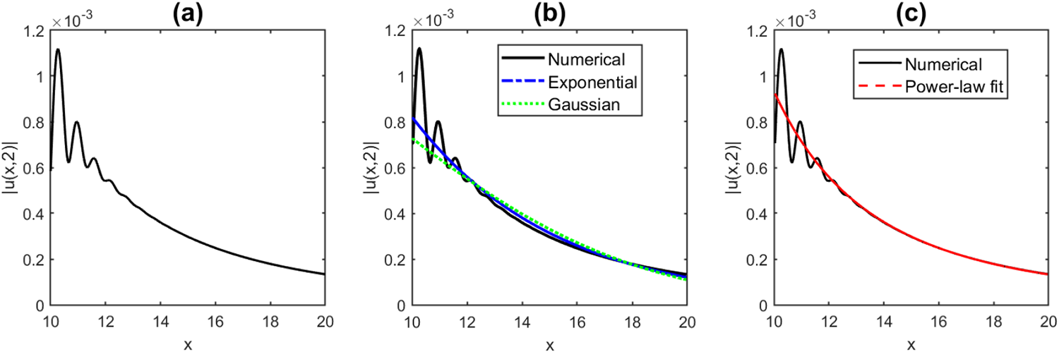
Numerical profile and asymptotic tail analysis of the similariton at the propagation distance $z=2$ for $\alpha=1.8$ near tail. (a) Numerical profile $\vert u(x,2)\vert$, (b) comparison of the numerical tail with the exponential and Gaussian decay models in the tail region $(10 \lt x \lt 20)$ and (c) comparison of the numerical tail with power-law model in the tail region $(10 \lt x \lt 20)$.

Figure 17 Long description

A line graph with the horizontal axis labeled x, ranging from 10 to 20 with tick labels at 10, 12, 14, 16, 18 and 20. The vertical axis is labeled with a scale factor, times 10 superscript negative 3 and tick labels at 0, 0.2, 0.4, 0.6, 0.8, 1.0 and 1.2. A single curve decreases from near 1.0 times 10 superscript negative 3 at x equals 10 to near 0.2 times 10 superscript negative 3 at x equals 20. The image B showing a line graph with the horizontal axis labeled x, ranging from 10 to 20 with tick labels at 10, 12, 14, 16, 18 and 20. The vertical axis is labeled with a scale factor, times 10 superscript negative 3 and tick labels at 0, 0.2, 0.4, 0.6, 0.8, 1.0 and 1.2. A legend lists Numerical, Exponential and Gaussian. Three curves decrease from near 1.0 times 10 superscript negative 3 at x equals 10 to near 0.2 times 10 superscript negative 3 at x equals 20, with the curves closely overlapping across the range. The image C showing a line graph with the horizontal axis labeled x, ranging from 10 to 20 with tick labels at 10, 12, 14, 16, 18 and 20. The vertical axis is labeled with a scale factor, times 10 superscript negative 3 and tick labels at 0, 0.2, 0.4, 0.6, 0.8, 1.0 and 1.2. A legend lists Numerical and Power law fit. Two curves decrease from near 1.0 times 10 superscript negative 3 at x equals 10 to near 0.2 times 10 superscript negative 3 at x equals 20, with the two curves separated for part of the range.

The behaviour of the tail is analysed in detail for different models. Figure 14(a) illustrates the specific section of the numerically obtained tail within the range of 15–30 for $\alpha=2$ and $g=0.5,x_0=1$. To further evaluate its asymptotic behaviour, Fig. 14(b) and (c) present a comparison of the numerical tail with exponential, Gaussian and power-law fitting functions. Within the selected interval of $15 \lt x \lt 30$, the exponential model provides a better approximation of the numerical tail than the Gaussian and power-law models.

To investigate the tail behaviour of the similaritons for various fractional orders $\alpha$, both the near and far tails are plotted at a fixed gain of $g = 0.5$ and a propagation distance of $z = 2$. Figure 15(a) corresponds to $\alpha = 1.1, 1.3$ and $1.4$, whereas Fig. 15(b) displays the results for $\alpha = 1.5, 1.6,$ and $1.8$. In these figures, the main panels present the near tails as a function of $x$, while the insets display the far tails of the similaritons.

For $1 \lt \alpha \le 1.5$, the solutions remain well localized but exhibit markedly different asymptotic behaviours. As shown in the left panel (Fig. 15a), the far tails decay algebraically, producing slowly decaying, long-range wings that become increasingly pronounced as $\alpha$ decreases.

Conversely, as $\alpha$ increases towards the classical limit ( $\alpha = 2$), shown in Fig. 15(b), spatial localization becomes significantly stronger. The algebraic tails are progressively suppressed, and the solutions approach an exponentially localized profile with negligible far-field amplitude. This transition is clearly visible in the inset, where the tail amplitude decreases by nearly an order of magnitude as $\alpha$ varies from $1.5$ to $1.8$.

Figure 16 compares the fitted models for $\alpha = 1.4$. As the figure shows, the power-law model provides a significantly better approximation to the numerical tail than the Gaussian and exponential models over the selected interval $5 \lt x \lt 30$.

We have numerically analysed the tail behaviour of the similariton for $\alpha = 1.8$. As $\alpha$ approaches the classical limit ( $\alpha \to 2$), the tail profile can be closely approximated by power-law fitting function. As seen in Fig. 17, for small values of $x$ close to the core region, the tail exhibits distinct oscillations, which we refer to as the near tail. These near-tail oscillations are the fractional counterpart of optical wave-breaking: as the chirped pulse reshapes, its steep flanks shed dispersive waves that interfere and produce ringing, as in the classical normal-dispersion wave-breaking of  [Reference Anderson, Desaix, Lisak and Quiroga-Teixeiro2, Reference Anderson, Desaix, Lisak and Quiroga-Teixeiro3], here carried by the oscillatory fractional propagation kernel. The effect is already present in the linear dynamics and is strongly enhanced by the Kerr reshaping; it is most pronounced near $\alpha=2$, where the pulse is closest to the wave-breaking regime while still retaining a genuinely fractional, oscillatory kernel. These are transient oscillations shed during propagation: the stationary tails of fractional coherent structures with $1 \lt \alpha \lt 2$ are purely algebraic and non-oscillatory [Reference Decker, Demirkaya, Alexander, Tsolias and Kevrekidis8, Reference Secchi30], with oscillatory-decaying tails arising only in the biharmonic regime $\alpha \gt 2$ [Reference Decker, Demirkaya, Alexander and Kevrekidis7, Reference Decker, Demirkaya, Alexander, Tsolias and Kevrekidis8].

Even as we move into the far-tail regime, the algebraic decay persists, and the numerically obtained profile is best fitted by the power-law function, confirming that fractional effects remain non-negligible even close to the classical limit.