2. Mathematical formulation

2.1. Flow configuration

In a system of Cartesian coordinates $ (x^{*},y^{*} )$ (see figure 1), consider a horizontal layer of incompressible Newtonian fluid film with density $\rho$ , dynamic viscosity $\mu$ and thickness $d$ flowing on an infinite flat plate. The asterisk denotes the dimensional variables. The plate oscillates in the $x^{*}$ -direction with its velocity magnitude given by

(2.1) \begin{equation} U_{p}^{*} \left (t^{*} \right ) =U_{1}\cos \left (\omega _{1} t^{*}\right )+U_{2}\cos \left (\omega _{2} t^{*}\right )\!, \end{equation}

where $U_{1}$ and $U_{2}$ are the superimposed constant velocity amplitudes, and $\omega _{1}$ and $\omega _{2}$ are considered two incommensurable frequencies. Two separate modes that contain no phase shifts are superimposed into the oscillation, and each mode has its own frequency and amplitude. When the liquid film remains stationary, the thickness of the film is $d$ . The upper free surface of the film is described by $y^{*}=\eta ^{*}(x^{*},t^{*})$ , and is covered by a monolayer of insoluble surfactant. We note ${\boldsymbol{V}}^{*}=(U^{*},V^{*})$ , where ${\boldsymbol{V}}^{*}$ is the velocity field, $U^{*}$ and $V^{*}$ are the velocity components in the streamwise and vertical directions. For the two-dimensional stability problem, the surfactant concentration $\mathit{\varGamma }^{*}(x^{*},t^{*})$ obeys the transport equation (Halpern & Frenkel Reference Halpern and Frenkel2003)

(2.2) \begin{equation} \frac {\partial \left (H \mathit{\varGamma }^{*} \right ) }{\partial t^{*} } +\frac {\partial }{\partial x^{*} } \left (H\mathit{\varGamma }^{*} U^{*} \right )=D_{s}\frac {\partial }{\partial x^{*} }\Biggl (\frac {1}{H}\frac {\partial \mathit{\varGamma }^{*}}{\partial x^{*} } \Biggr ), \end{equation}

where $H=\sqrt {1+ ( {\partial \eta ^{*} }/{\partial x^{*} } )^{2} }$ is the curvature parameter associated with the free upper surface of the fluid film. Here $D_{s}$ is the diffusivity of the surfactant, which is usually negligible and is ignored below. For the infinitesimal disturbance at the free surface, the precise nature of the dependence of surface tension $\sigma ^{*}$ and the surfactant concentration $\mathit{\varGamma }^{*}(x^{*},t^{*})$ is a linear relation

(2.3) \begin{equation} \sigma ^{*}=\sigma _{0}-E\left (\mathit{\varGamma } ^{*} -\mathit{\varGamma }_{0} \right ) , \end{equation}

where $E$ is the surface elasticity, and $\mathit{\varGamma }_{0}$ is the basic value of the surfactant concentration, corresponding to a uniform surface tension $\sigma _{0}$ .

The system of the governing equations is given by the following momentum and continuity equations:

(2.4) \begin{align} \rho \left (\frac {\partial }{\partial t^{*} } +{\boldsymbol{V}} ^{*} \boldsymbol{\cdot }\boldsymbol{\nabla }\right ){\boldsymbol{V}} ^{*} &=-\boldsymbol{\nabla }P^{*}+\mu {\nabla} ^{2}{\boldsymbol{V}} ^{*}+\rho {\boldsymbol{g}}, \end{align}

(2.5) \begin{align} \boldsymbol{\nabla }\boldsymbol{\cdot }{\boldsymbol{V}} ^{*}&=0. \end{align}

Here $P^{*}$ is the isotropic pressure and $\boldsymbol{g}$ represents the acceleration due to gravity.

The corresponding boundary conditions are

1. (i) at the bottom of liquid film $y^*=-d$ ,

   (2.6) \begin{equation} U^{*}=U_{p}^{*}\left (t^{*}\right )\!,\quad V^{*}=0; \end{equation}

2. (ii) the kinematic boundary condition at the free surface,

   (2.7) \begin{equation} \frac {\partial \eta ^{*}}{\partial t^{*}} =V^{*}-U^{*} \frac {\partial \eta ^{*} }{\partial x^{*} }; \end{equation}

3. (iii) the normal and tangential stresses at the free surface,

   (2.8a) \begin{align} \mu\! \Bigg [\left (1-\left (\frac {\partial \eta ^{*} }{\partial x^{*}}\right )^{2}\right )\left (\frac {\partial U^{*} }{\partial y^{*}} +\frac {\partial V^{*}}{\partial x^{*}} \right ) + 2\frac {\partial \eta ^{*} }{\partial x^{*}}&\left (\frac {\partial V^{*}}{\partial y^{*}}-\frac {\partial U^{*}}{\partial x^{*}}\right )\Bigg ]\notag \\ &=\sqrt {1+\left (\frac {\partial \eta ^{*} }{\partial x^{*}}\right )^{2}} \frac {\partial \sigma ^{*}}{\partial x^{*}} , \end{align}
   (2.8b) \begin{align} -\left (1+\left (\frac {\partial \eta ^{*} }{\partial x^{*}}\right )^{2}\right )P^{*}+2\mu \Biggl [\left (\frac {\partial \eta ^{*} }{\partial x^{*}}\right )^{2}\frac {\partial U^{*}}{\partial x^{*}} -\frac {\partial \eta ^{*} }{\partial x^{*}}\biggl (&\frac {\partial U^{*}}{\partial y^{*}}+\frac {\partial V^{*}}{\partial x^{*}}\biggr )+\frac {\partial V^{*}}{\partial y^{*}}\Biggr ]\notag \\ &=\frac {\sigma ^{*}\frac {\partial ^{2} \eta ^{*}}{\partial x^{*2}} }{\sqrt {1+\left (\frac {\partial \eta ^{*} }{\partial x^{*}}\right )^{2}} }, \end{align}

where $\sigma ^{*}$ is the surface tension.

To non-dimensionalize the governing equations and boundary conditions, we introduce the following dimensionless variables and we choose the parameters of the first modes as the characteristic scales. The mean thickness of liquid film $d$ is selected as the characteristic length scale, $U_{1}$ as the velocity scale, $\omega _{1}^{-1}$ as the time scale and $\rho U_{1}^{2}$ as the pressure scale. The surfactant concentration and surface tension are normalized by $\mathit{\varGamma }_{0}$ and $\sigma _{0}$ . In addition, multiple velocity scales can be chosen, such as $U_{1}$ and ${\rm d}\omega _{1}$ . Here $U_{1}$ represents the maximum velocity amplitude of the oscillating plate, which characterizes the intensity of the momentum input into the fluid forced motion in the system. With $U_{1}$ , the impact of velocity on flow behaviour can be quantified, and this non-dimensionalization approach facilitates the comparison of inertial and viscous effects. On the other hand, ${\rm d}\omega _{1}$ is non-dimensionalized based on characteristic length and oscillation frequency, emphasizing the time scale characteristics dominated by geometry and frequency rather than the actual velocity amplitude in the system. Actually, both non-dimensional variables are applicable. After comparing the results from different non-dimensionalized velocity variables, we found that using $U_{1}$ yields a more concise and straightforward form of the governing equations and boundary conditions, more effectively capturing the driving mechanisms of the system. Therefore, $U_{1}$ is chosen as the velocity scale in this study. It should be noted that while the choice of non-dimensional variable does not alter the overall results, it does affect the coefficients of the terms in the governing equations.

Then, a set of dimensionless parameters are obtained as follows:

(2.9) \begin{align} Re=\frac {U_{1}d}{\nu }, \qquad \chi =\frac {gd^{3}}{2\nu ^{2}}, \qquad \beta =&\sqrt {\frac {\omega _{1}d^{2}}{2\nu }},\qquad Ca=\frac {\mu U_{1}}{\sigma _{0}}, \qquad Ma=\frac {E\mathit{\varGamma }_{0}}{\sigma _{0}},\notag \\ M=\frac {E\mathit{\varGamma }_{0}}{\rho U_{1}^{2}d}, \qquad &\omega =\frac {\omega _{2}}{\omega _{1}},\qquad \gamma =\frac {U_{2}}{U_{1}}, \end{align}

where $\nu =\mu /\rho$ is the kinematic viscosity. Here $Re$ is the Reynolds number, which measures the ratio of the inertial effect, due to the oscillation amplitude $U_{1}$ to the viscous effect, and $\chi$ is the Galileo number, which interprets the ratio of the gravity effect to the viscous effect. Here $\beta$ is the Womersley number, which is the dimensionless frequency parameter representing the ratio of the average film thickness to the thickness of the Stokes layer induced by the wall oscillation, and it is also interpreted as a measure of the relative oscillation frequency $\omega _{1}$ . Here $Ca$ represents the capillary number, which characterizes the ratio of the viscous force to the surface tension force. The Marangoni number $Ma$ shows the ratio of the surface-tension gradient force to the viscous force and $M$ here is introduced to quantify the influence of surface surfactant. At last, $\gamma =U_{2}/U_{1}$ is the ratio of superimposed velocity amplitudes and $\omega = \omega _{2}/\omega _{1}$ is the frequency ratio considered irrational. These two parameters are crucial in this paper for describing quasiperiodic oscillations.

Substituting these dimensionless variables into (2.4)–(2.8), we obtain the following dimensionless system:

(2.10a) \begin{align} \frac {2\beta ^{2} }{\textit{Re}} \frac {\partial U}{\partial t} +U\frac {\partial U}{\partial x} +V\frac {\partial U}{\partial y}&=-\frac {\partial P}{\partial x}+\frac {1}{{\textit{Re}}^{2} }\left (\frac {\partial ^{2} U}{\partial x^{2} } +\frac {\partial ^{2} U}{\partial y^{2} }\right )\!, \\[-12pt]\nonumber\end{align}

(2.10b) \begin{align} \frac {2\beta ^{2} }{\textit{Re}} \frac {\partial V}{\partial t} +U\frac {\partial V}{\partial x} +V\frac {\partial V}{\partial y}&=-\frac {\partial P}{\partial y}+\frac {1}{{\textit{Re}}^{2} }\left (\frac {\partial ^{2} V}{\partial x^{2} } +\frac {\partial ^{2} V}{\partial y^{2} }\right ) -\frac {2\chi }{{\textit{Re}}^{2}} , \\[-12pt]\nonumber\end{align}

(2.11) \begin{align} \frac {\partial U}{\partial x} +\frac {\partial V}{\partial y}&=0 . \end{align}

Here $(U,V)$ are the dimensionless components of the velocity field ${\boldsymbol{V}}(x,y,t)$ . It is noted that the coefficient appearing before the temporal term, $2\beta ^{2} /Re$ , is equivalent to $2\omega _{1}d/U_{1}$ . We also obtain the following dimensionless equations of the boundary conditions. The boundary conditions at the horizontal wall $y=-1$ , in a dimensionless form are

(2.12) \begin{equation} U=U_{p}\left (t\right )\!,\ \ \ V=0, \end{equation}

and the dimensionless velocity of the horizontal wall is given by

(2.13) \begin{equation} U_{p}\left (t\right )=\cos \left (t\right )+\gamma \cos \left (\omega t\right )\!, \end{equation}

when the ratio of the velocity amplitudes $\gamma$ is zero, we are in configuration studied by Gao & Lu (Reference Gao and Lu2006). The dimensionless form of the transport equation of the surfactant concentration and the relation between the surfactant concentration and the surface tension are as follows:

(2.14) \begin{align}& \frac {2\beta ^{2} }{\textit{Re}} \frac {\partial \left (H\mathit{\varGamma } \right )}{\partial t} +\frac {\partial }{\partial x} \left (H\mathit{\varGamma } U\right )=0, \\[-12pt]\nonumber \end{align}

(2.15) \begin{align}&\qquad\,\, \sigma =1-Ma\left (\mathit{\varGamma } -1\right )\!. \end{align}

The boundary conditions at the free surface, $y=\eta (x,t)$ , in a dimensionless form are as follows:

(2.16a) \begin{align} V=\biggl (\frac {2\beta ^{2} }{\textit{Re}}& \frac {\partial }{\partial t} +U\frac {\partial }{\partial x} \biggr )\eta , \end{align}

(2.16b) \begin{align} \frac {1}{\sqrt {1+\left (\frac {\partial \eta }{\partial x} \right )^{2}} } \Biggl [\left (1-\left (\frac {\partial \eta }{\partial x} \right )^{2}\right )\left (\frac {\partial U}{\partial y}+\frac {\partial V}{\partial x} \right )&+2\left (\frac {\partial \eta }{\partial x} \right )^{2}\left (\frac {\partial V}{\partial y}-\frac {\partial U}{\partial x} \right )\Biggr ]=-\frac {\textit{Ma}}{\textit{Ca}}\frac {\partial \mathit{\varGamma } }{\partial x}, \end{align}

(2.16c) \begin{align} -P+P_{0} +\frac {2}{Re\left (1+\left (\frac {\partial \eta }{\partial x} \right )^{2}\right )} \Biggl [&\frac {\partial V}{\partial y} +\left (\frac {\partial \eta }{\partial x} \right )^{2}\frac {\partial U}{\partial x} -\frac {\partial \eta }{\partial x}\left (\frac {\partial U}{\partial y}+\frac {\partial V}{\partial x} \right ) \Biggr ]\notag \\ &= \frac { \frac {\partial ^{2} \eta }{\partial x^{2} } }{\sqrt {\left (1+\left (\frac {\partial \eta }{\partial x} \right )^{2}\right )^{3}} }\frac {1-Ma\left (\mathit{\varGamma } -1\right )}{\textit{ReCa}}, \end{align}

where $P_{0}$ is the dimensionless reference pressure at the interface.

The basic state corresponds to a plane interface flow with a unidirectional velocity parallel to the $x$ axis, and ${\boldsymbol{V}} _{b}=(U_{b}(y,t),\ 0)$ . The characteristic pressure is fixed by the disturbance problem, given that the base flow has a zero pressure gradient. By the method of separation of variables, we obtain the dimensionless form of the basic velocity profile

(2.17) \begin{align}& U_{b}=\mathrm{Re} \left [\frac {\cosh r_{1}y}{\cosh r_{1}}\mathrm{e}^{{i}t} +\gamma \frac {\cosh r_{2}y}{\cosh r_{2}}\mathrm{e}^{{i}\omega t} \right ]\!, \end{align}

(2.18) \begin{align}&\qquad\qquad\quad \bar {P}\left (y\right ) =P_{0}-\frac {2\chi }{{\textit{Re}}^{2}}y, \end{align}

where $-1 \leqslant y\leqslant 0$ , $r_{1}=(1+\mathrm{i})\beta$ and $r_{2}=(1+\mathrm{i})\beta \sqrt {\omega }$ . Here $\mathrm{Re}[\boldsymbol{\cdot }]$ represents the real part of that complex function. Three parameters are involved in the expression of the base flow profile: the ratio of the velocity amplitudes $\gamma$ , the frequency ratio $\omega$ and the parameter  $\beta$ . The expression for $U_{b}$ does not include the parameter $Ma$ , which characterizes the presence of surfactants, and that means the surfactant has no effect on the basic flow. This is based on the assumption that the initial distribution of surfactants at the interface is uniform. Under this assumption, no surfactant concentration gradients develop in the base state, and consequently no Marangoni stresses arise to modify the flow field.

2.2. Linear stability problem

In order to study the linear stability of the base flow, infinitesimal perturbations are superimposed on the fundamental flow by introducing the following variables:

(2.19) \begin{equation} U=U_{b}+u',\quad V=v', \quad P=\bar {P}+p', \quad \varGamma =1+\varGamma ', \quad \sigma =1+\sigma '. \end{equation}

Here $(u',v')$ are the components of the velocity disturbance in the Cartesian coordinates $ (x,y )$ . Here $p'$ and $\eta '$ designate pressure and interface disturbances, and $\mathit{\varGamma }'$ and $\sigma '$ designate surfactant concentration and surface tension disturbances, respectively.

Since only two-dimensional perturbations are considered, the continuity equation (2.5) is automatically satisfied by introducing a perturbed stream function $\psi ' (x,y )$ , such that

(2.20) \begin{equation} u'=\frac {\partial \psi ^{\prime }}{\partial y} ,\qquad v'=-\frac {\partial \psi ^{\prime }}{\partial x} . \end{equation}

The state of the base flow is independent of $x$ . Thereafter, the perturbations of the stream function $\psi '$ , surfactant concentration $\mathit{\varGamma }'$ and interface $\eta '$ are written in normal modes, i.e.

(2.21) \begin{equation} \left (\psi ',\ \mathit{\varGamma }',\ \eta '\right )=\left (\phi \left (y,t\right )\!,\ \xi \left (t\right )\!,\ h\left (t\right )\right )\mathrm{e}^{{i}kx}, \end{equation}

where $k\in \mathbb{R}$ is the wavenumber in the streamwise direction. Note that the pressure $p'$ can be eliminated by combining the Navier–Stokes equations, and hence it does not appear in the linearized system. Substituting (2.21) into the governing equations and linearizing, we obtain the time-dependent Orr–Sommerfeld equation

(2.22) \begin{align} \left (\frac {2\beta ^{2} }{\textit{Re}} \frac {\partial }{\partial t} +\mathrm{i}kU_{b}\right )\left (\frac {\partial ^{2} }{\partial y^{2}}-k^{2}\right )\phi -\mathrm{i}k\frac {\partial ^{2} U_{b}}{\partial y^{2}}\phi =\frac {1}{\textit{Re}}\left (\frac {\partial ^{4} \phi }{\partial y^{4}}-2k^{2}\frac {\partial ^{2}\phi }{\partial y^{2}}+k^{4}\phi \right )\! . \end{align}

Substituting the normal modes (2.21) and linearizing, the boundary conditions at the wall $y=-1$ are

(2.23) \begin{equation} \phi =\frac {\partial \phi }{\partial y}=0. \end{equation}

The linearized kinematic boundary condition and transport equation for surfactant are expressed by

(2.24) \begin{align} \frac {2\beta ^{2}}{\textit{Re}} \frac {\mathrm{d} h}{\mathrm{d} t} +\mathrm{i}kU_{b}h+\mathrm{i}k\phi &=0, \\[-12pt]\nonumber \end{align}

(2.25) \begin{align} \frac {2\beta ^{2}}{\textit{Re}} \frac {\mathrm{d} \xi }{\mathrm{d} t} +\mathrm{i}kU_{b}\xi +\mathrm{i}k\frac {\partial \phi }{\partial y} &=0. \end{align}

The linearized conditions for the normal and tangential stresses at $y=0$ are given by

(2.26) \begin{align} \frac {\partial ^{2} U_{b}}{\partial y^{2}} h+\frac {\partial ^{2} \phi }{\partial y^{2}}+k^{2}\phi &+\frac {\textit{Ma}}{\textit{Ca}}\mathrm{i}k\xi =0, \\[-12pt]\nonumber \end{align}

(2.27) \begin{align} \frac {2\beta ^{2}}{\textit{Re}} \frac {\partial ^2 \phi }{\partial t\partial y}-\frac {1}{\textit{Re}} \left (\frac {\partial ^{2} }{\partial y^{2}} -3k^{2}\right )\frac {\partial \phi }{\partial y} +\mathrm{i}kU_{b}&\frac {\partial \phi }{\partial y}+\mathrm{i}k\left (\frac {2\chi }{{\textit{Re}}^{2}} +\frac {k^{2}}{\textit{ReCa}} \right )h=0. \end{align}

The Floquet system (2.22)–(2.27) governs the linear stability problem and is formally consistent with that in Gao & Lu (Reference Gao and Lu2006) and Gao & Lu (Reference Gao and Lu2008). However, due to the presence of quasiperiodic oscillations, the base flow in the present study differs from that in the previous work. For finite-wavelength instabilities, the differential system should be solved numerically, while long-wavelength solutions can be analytically obtained by an expansion in $k$ and will be discussed in the following section.

3. The long-wavelength expansion

While Floquet theory provides a powerful framework for analysing the stability of linear differential systems with periodic coefficients, it becomes inadequate in the presence of systems characterized by two incommensurate frequencies, $\omega _{1}$ and $\omega _{2}$ . In such quasiperiodic systems, the absence of a common period invalidates the fundamental assumptions underpinning Floquet analysis. Consequently, we use the approximation that consists of rendering an irrational number, $\omega$ , into a rational one (Jaouahiry & Aniss Reference Jaouahiry and Aniss2025). We introduce the following variable changes:

(3.1) \begin{equation} \omega =\frac {p}{q} ,\qquad \tau =\frac {t}{q} ,\qquad \frac {\partial }{\partial t} =\frac {1}{q} \frac {\partial }{\partial \tau }, \end{equation}

where $p$ and $q$ are prime integers. Under the limit of long wave perturbations, the wavenumber $k$ is considered as a small parameter and the solution can be expressed as follows:

(3.2a) \begin{align} \phi \left (y,\tau \right )&=\mathrm{e}^{\lambda \tau }\left [\phi _{0}\left (y,\tau \right )+k\phi _{1}\left (y,\tau \right )+k^{2}\phi _{2}\left (y,\tau \right )+{\cdots} \right ]\!, \\[-12pt]\nonumber \end{align}

(3.2b) \begin{align} h\left (\tau \right )&=\mathrm{e}^{\lambda \tau }\left [h _{0}\left (\tau \right )+kh _{1}\left (\tau \right )+k^{2}h _{2}\left (\tau \right )+{\cdots} \right ]\!, \\[-12pt]\nonumber \end{align}

(3.2c) \begin{align} \xi \left (\tau \right )&=\mathrm{e}^{\lambda \tau }\left [\xi _{0}\left (\tau \right )+k\xi _{1}\left (\tau \right )+k^{2}\xi _{2}\left (\tau \right )+{\cdots} \right ]\!, \end{align}

where $\phi _{j}(y,\tau )$ , $h_{j}(\tau )$ and $\xi _{j}(\tau )$ ( $j=0,1,2,\ldots$ ) are $2\pi$ -periodic in time, and $\lambda =\lambda _{r}+\mathrm{i}\lambda _{{i}}$ is the complex growth rate of the disturbance, also named the Floquet exponent, and $\lambda$ can be expanded as a power series in $k$ :

(3.3) \begin{equation} {\lambda } =\lambda _{0}+k\lambda _{1}+k^{2}\lambda _{2}+{\cdots} . \end{equation}

Substituting these expansions into the Floquet system and collecting like terms with different order, a set of coupled equations for $\phi _{j}$ , $h_{j}$ and $\xi _{j}$ will be obtained, and the equations can be solved sequentially. The purpose of this procedure is to find the first non-zero $\lambda _{j}$ , corresponding to exponential growth or decay of the disturbance.

For the first order $O(1)$ , the Orr–Sommerfeld equation and boundary conditions are then given by

(3.4) \begin{align} \frac {\partial ^{4} \phi _{0} }{\partial y^{4}}-\frac {2\beta ^{2} }{q}\frac {\partial ^3 \phi _{0}}{\partial \tau \partial y^{2}}&-\frac {2\beta ^{2} }{q} \lambda _{0}\frac {\partial ^{2}\phi _{0}}{\partial y^{2}} =0, \end{align}

(3.5) \begin{align} \phi _{0}=0,\quad \frac {\partial \phi _{0}}{\partial y}& =0\qquad \text{ at } y=-1, \end{align}

(3.6) \begin{align} \frac {\mathrm{d} h_{0} }{\mathrm{d} \tau } +\lambda _{0} h_{0} &=0\qquad \text{ at } y=0, \end{align}

(3.7) \begin{align} \frac {\mathrm{d} \xi _{0} }{\mathrm{d} \tau } +\lambda _{0} \xi _{0} &=0\qquad \text{ at } y=0, \end{align}

(3.8) \begin{align} \frac {\partial ^{2}\phi _{0}}{\partial y^{2}}+ \frac {\partial ^{2}U_{b}}{\partial y^{2}}h_{0}&=0\qquad \text{ at } y=0, \end{align}

(3.9) \begin{align} \frac {\partial ^{3}\phi _{0}}{\partial y^{3}}-\frac {2\beta ^{2} }{q} \frac {\partial ^{2}\phi _{0}}{\partial \tau \partial y}-\frac {2\beta ^{2} }{q}&\lambda _{0} \frac {\partial \phi _{0} }{\partial y}=0\qquad \text{ at } y=0. \end{align}

Since $h_{0}(\tau )$ and $\xi _{0}(\tau )$ are both time-periodic functions of $\tau$ , the kinematic condition (3.6) and the transport equation for surfactant (3.7) lead to an admissible solution $\lambda _{0}=0$ . And $h_{0}$ and $\xi _{0}$ are constant. Solving (3.4)–(3.9), the first-order solution can be expressed as follows:

(3.10) \begin{equation} \phi _{0}(y,\tau )=h_{0}{\rm Re} \left [\frac {1-\cosh r_{1}\left (y+1\right )}{\cosh ^{2}r_{1}}\mathrm{e}^{{i}q\tau } +\gamma \frac {1-\cosh r_{2}\left (y+1\right )}{\cosh ^{2}r_{2}}\mathrm{e}^{{i}p\tau } \right ]\!. \end{equation}

Obviously, in this order, $\phi _{0}(y,\tau )$ depends on the ratio of the amplitudes of the quasiperiodic modulation $\gamma =U_{2}/U_{1}$ and the surface surfactant does not affect the velocity distribution at this order.

For order $O(k)$ , the Orr–Sommerfeld equation and boundary conditions are then given by

(3.11) \begin{align} \frac {\partial ^{4} \phi _{1} }{\partial y^{4} } -\frac {2\beta }{q} \biggl ( \frac {\partial ^{3} \phi _{1} }{\partial \tau \partial y^{2} }+\lambda _{1}&\frac {\partial ^{2} \phi _{0}}{\partial y^{2}}\biggr )=\mathrm{i}Re\biggl (U_{b}\frac {\partial ^{2} \phi _{0}}{\partial y^{2}}-\frac {\partial ^{2} U_{b}}{\partial y^{2}}\phi _{0} \biggr ), \end{align}

(3.12) \begin{align} \phi _{1}=0,\quad &\frac {\partial \phi _{1}}{\partial y}=0\qquad \text{ at } y=-1, \end{align}

(3.13) \begin{align} \frac {2\beta ^{2} }{q} \biggl (\frac {\mathrm{d} h_{1} }{\mathrm{d} \tau } +\lambda _{1}h_{0} \biggr )+\mathrm{i}Re&\phi _{0} +\mathrm{i}ReU_{b}h_{0} =0\qquad \text{ at } y=0, \end{align}

(3.14) \begin{align} \frac {2\beta ^{2} }{q} \biggl (\frac {\mathrm{d} \xi _{1} }{\mathrm{d} \tau } +\lambda _{1}\xi _{0} \biggr )+\mathrm{i}Re&\frac {\partial \phi _{0}}{\partial y} +\mathrm{i}ReU_{b}\xi _{0} =0\qquad \text{ at } y=0, \end{align}

(3.15) \begin{align} \frac {\partial ^{2} \phi _{1} }{\partial y^{2} } +\frac {\partial ^{2} U_{b} }{\partial y^{2} }h_{1}+&\mathrm{i}\frac {\textit{Ma}}{\textit{Ca}} \xi _{0}=0\qquad \text{ at } y=0, \end{align}

(3.16) \begin{align} \frac {\partial ^{3} \phi _{1} }{\partial y^{3} } -\frac {2\beta ^{2} }{q} \biggl ( \frac {\partial ^{2}\phi _{1} }{\partial \tau \partial y}+\lambda _{1}\frac {\partial \phi _{0} }{\partial y}\biggr )&=\mathrm{i}ReU_{b}\frac {\partial \phi _{0} }{\partial y}+\mathrm{i}\frac {2\chi }{\textit{Re}} h_{0}\qquad \text{ at } y=0. \end{align}

Since $\phi _{0}$ and $U_{b}$ are time periodic with a zero average, to obtain periodic solutions $h_{1}(\tau )$ and $\xi _{1}(\tau )$ , we must have $\lambda _{1}=0$ to ensure that $h_{1}(\tau )$ and $\xi _{1}(\tau )$ have periodic solutions. Then the expression of $h_{1}(\tau )$ and $\xi _{1}(\tau )$ can be obtained, as follows:

(3.17) \begin{align} h_{1}=&\frac{{\textit{Re}}h_{0} }{r_{1}^{2} } \mathrm{Im} \left [\frac {1}{\cosh ^{2} r_{1}}\mathrm{e}^{{i}q\tau }\right ]+\gamma \frac{{\textit{Re}}h_{0} }{r_{2}^{2} } \mathrm{Im} \left [\frac {1}{\cosh ^{2} r_{2}}\mathrm{e}^{{i}p\tau }\right ]\!, \\[-12pt]\nonumber\end{align}

(3.18) \begin{align} \xi _{1} =&\frac{{\textit{Re}}\xi _{0}}{r_{1}^{2} } \mathrm{Im} \left [\frac {1}{\cosh r_{1} }\mathrm{e}^{{i}q\tau } \right ]+\gamma \frac{{\textit{Re}}\xi _{0}}{r_{2}^{2} } \mathrm{Im} \left [\frac {1}{\cosh r_{2} }\mathrm{e}^{{i}p\tau } \right ] \notag \\ \\[-12pt]\nonumber&-\frac{{\textit{Re}}h_{0}}{r_{1}^{2} } \mathrm{Im} \left [\frac {r_{1}\sinh r_{1}}{\cosh ^{2} r_{1} }\mathrm{e}^{{i}q\tau } \right ]-\gamma \frac{{\textit{Re}}h_{0}}{r_{2}^{2} } \mathrm{Im} \left [\frac {r_{2}\sinh r_{2}}{\cosh ^{2} r_{2} }\mathrm{e}^{{i}p\tau }\right ]\!. \end{align}

Here $\mathrm{Im}[\boldsymbol{\cdot }]$ represents the imaginary part of that complex function. The solution of (3.11) is written in the form

(3.19) \begin{align} \phi _{1} \left (y,\tau \right )=\psi _{1} \left (y\right )\mathrm{e}^{2{i}q\tau } +\psi _{2} \left (y\right )\mathrm{e}^{-2{i}q\tau } +\psi _{3} \left (y\right )\mathrm{e}^{2{i}p\tau } +\psi _{4} \left (y\right )\mathrm{e}^{-2{i}p\tau }+\psi _{5}(y) . \end{align}

The differential system for $\phi _{1}$ contains inhomogeneous terms which are products of functions having a time dependence given by $\mathrm{e}^{\pm 2{i}q\tau }$ or $\mathrm{e}^{\pm 2{i}p\tau }$ . Therefore, $\psi _{5}(y)$ denotes the steady part in (3.19). As will be shown later, it is sufficient to solve for $\psi _{5}(y)$ to obtain $\lambda _{2}$ and hence to determine the stability of the flow. The corresponding time-independent system is

(3.20) \begin{align} &\frac {{d}^{4} \psi _{5} }{{\rm d} y^{4} } = \mathrm{i}{\textit{Reh}}_{0} {\rm Re} \Biggl [\frac {2\cosh r_{1}y\cos r_{1}\left (y+1\right )-\cosh r_{1}y}{2r_{1}^{-2}\cos ^{2}r_{1}\cosh r_{1} } \notag \\ &\qquad\quad +\gamma ^{2} \frac {2\cosh r_{2}y\cos r_{2}\left (y+1\right )-\cosh r_{2}y}{2r_{2}^{-2}\cos ^{2}r_{2}\cosh r_{2} } \Biggr ], \end{align}

(3.21) \begin{align} &\qquad\qquad\qquad \psi _{5}\left (-1\right )=\frac {\mathrm{d} \psi _{5}\left (-1\right )}{\mathrm{d} y} =0, \end{align}

(3.22) \begin{align} \frac {{d}^{2} \psi _{5}\left (0\right ) }{\mathrm{d} y^{2} } &+\mathrm{i}{\textit{Reh}}_{0} {\rm Re} \Biggl [\frac {1}{2\cos ^{2}r_{1}\cosh r_{1}}+\gamma ^{2}\frac {1}{2\cos ^{2}r_{2}\cosh r_{2}} \Biggl ]+\mathrm{i}\frac {\textit{Ma}}{\textit{Ca}} \xi _{0} =0, \end{align}

(3.23) \begin{align} \frac {{d}^{3} \psi _{5}\left (0\right ) }{\mathrm{d} y^{3} } &-\mathrm{i}{\textit{Reh}}_{0} {{\rm Re}} \Biggl [\frac {r_{1}\sin {r_{1}}}{2\cos ^{2} r_{1}\cosh r_{1}} +\gamma ^{2}\frac {r_{2}\sin {r_{2}}}{2\cos ^{2} r_{2}\cosh r_{2}}\Biggr ]-\mathrm{i}\frac {2\chi }{\textit{Re}} h_{0}=0. \end{align}

The solution to this system is represented by

(3.24) \begin{align} &\psi _{5} \left (y\right )=A_{0}+A_{1}y+A_{2}y^{2}+A_{3}y^{3}-\mathrm{i}{\textit{Reh}}_{0} {\rm Re} \notag \\ &\quad\times\left [\frac {2\cosh r_{1}y+\cosh r_{1}y\cos r_{1}\left (y+1\right )}{4r_{1}^{2}\cosh r_{1}\cos ^{2} r_{1}} +\gamma ^{2} \frac {2\cosh r_{2}y+\cosh r_{2}y\cos r_{2}\left (y+1\right )}{4r_{2}^{2}\cosh r_{2}\cos ^{2} r_{2}}\right ]\!. \end{align}

Here these four coefficients can be determined by the boundary conditions (3.21)–(3.23) and are expressed as

(3.25) \begin{align} A_{0}&=-\mathrm{i}\frac {2\chi }{3\textit{Re}} h_{0}-\mathrm{i}\frac {\textit{Ma}}{2\textit{Ca}} \xi _{0}+\mathrm{i}{\textit{Reh}}_{0} \mathrm{Re} \left [\!\frac {3\cosh r_{1}\!-\!3r_{1}\sinh r_{1}}{4r_{1}^{2}\cosh r_{1}\cos ^{2} r_{1}} +\gamma ^{2} \frac {3\cosh r_{2}\!-\!3r_{2}\sinh r_{2}}{4r_{2}^{2}\cosh r_{2}\cos ^{2} r_{2}} \!\right ]\!,\notag \\ A_{1}&=-\mathrm{i}\frac {\chi }{\textit{Re}}h_{0} -\mathrm{i}\frac {\textit{Ma}}{\textit{Ca}}\xi _{0} -\mathrm{i}{\textit{Reh}}_{0} \mathrm{Re} \left [\frac {3\sinh r_{1}}{4r_{1}\cosh r_{1}\cos ^{2} r_{1}} +\gamma ^{2} \frac {3\sinh r_{2}}{4r_{2}\cosh r_{2}\cos ^{2} r_{2}}\right ]\!,\notag \\ A_{2}&=-\mathrm{i}\frac {\textit{Ma}}{2Ca} \xi _{0}, \notag \\ A_{3}&=\mathrm{i}\frac {\chi }{3Re} h_{0}. \end{align}

For $O(k^{2})$ , the kinematic boundary condition and the surfactant transport equation are given by

(3.26) \begin{align} \frac {2\beta ^{2} }{qRe} \biggl (\frac {\mathrm{d} h_{2} }{\mathrm{d} \tau }+\lambda _{2} h_{0} \biggr )+\mathrm{i}U_{b}h_{1}+\mathrm{i}\phi _{1}&=0\qquad \text{ at } y=0, \end{align}

(3.27) \begin{align} \frac {2\beta ^{2} }{qRe} \biggl (\frac {\mathrm{d} \xi _{2} }{\mathrm{d} \tau }+\lambda _{2} \xi _{0} \biggr )+\mathrm{i}U_{b}\xi _{1}+\mathrm{i}\frac {\partial \phi _{1}}{\partial y} &=0\qquad \text{ at } y=0. \end{align}

By taking the steady terms on both sides, the expression of $\lambda _{2}$ is obtained from (3.26) and (3.27),

(3.28) \begin{align} \frac {2\beta ^{2} }{qRe} \lambda _{2} h_{0}=&-\frac {2\chi }{3{\textit{Re}}^{2}}h_{0} -\frac {\textit{Ma}}{2ReCa} \xi _{0} +I_{1}h_{0}, \\[-12pt]\nonumber\end{align}

(3.29) \begin{align} \frac {2\beta ^{2} }{qRe} \lambda _{2} \xi _{0}=&-\frac {\chi }{{\textit{Re}}^{2}}h_{0} -\frac {\textit{Ma}}{\textit{ReCa}} \xi _{0} +I_{2}h_{0}, \end{align}

where

(3.30) \begin{align} I_{1} &=\mathrm{Re} \Biggl [\frac {3\cosh r_{1}-3r_{1}\sinh r_{1}-\cos r_{1}}{4r_{1}^{2}\cosh r_{1} \cos ^{2}r_{1} } +\gamma ^{2} \frac {3\cosh r_{2}-3r_{2}\sinh r_{2}-\cos r_{2}}{4r_{2}^{2}\cosh r_{2}\cos ^{2}r_{2}} \Biggr ], \\[-12pt]\nonumber\end{align}

(3.31) \begin{align} I_{2} &=\mathrm{Re} \Biggl [\frac {3\sin r_{1}-3\sinh r_{1}}{4r_{1}\cosh r_{1}\cos ^{2}r_{1}}+\gamma ^{2} \frac {3\sin r_{2}-3\sinh r_{2}}{4r_{2}\cosh r_{2}\cos ^{2}r_{2}} \Biggr ]. \end{align}

Note that $I_{1}$ and $I_{2}$ depend on $\beta$ , $\omega$ and $\gamma$ . Equations (3.28) and (3.29) can be written in the matrix form

(3.32) \begin{equation} \begin{bmatrix} \displaystyle { I_1-\frac {2\chi }{3{\textit{Re}}^{2}}} &\quad \displaystyle { -\frac {1}{2}M }\\[10pt] \displaystyle { I_2 -\frac {\chi }{{\textit{Re}}^{2}}} &\quad \displaystyle { -M}\end{bmatrix} \begin{bmatrix}\displaystyle { h_0}\\ \displaystyle {\xi _0}\end{bmatrix}= \frac {2\beta ^2}{q{\textit{Re}}^{2}} \lambda _2\begin{bmatrix}h_0\\ \xi _0 \end{bmatrix}, \end{equation}

where the dimensionless number is

(3.33) \begin{equation} M=\frac {\textit{Ma}}{\textit{ReCa}}=\frac {E{\varGamma }_{0}}{\rho U_{1}^{2}d} \ . \end{equation}

The parameter $M$ can be regarded as the ratio of the Marangoni stress to the inertial force, represents the influence of surface surfactant. Obviously, (3.32) is an eigenvalue problem, with $2\beta ^{2}\lambda _{2}/q{\textit{Re}}^{2}$ being the eigenvalue and $[h_{0},\xi _{0}]^{T}$ the eigenvector. For clarity, let $\theta =2\beta ^{2}\lambda _{2}/q{\textit{Re}}^{2}$ , then $\theta$ can be obtained by solving the quadratic equation

(3.34) \begin{equation} \theta ^{2} +b\theta +c=0, \end{equation}

where the coefficients $b$ and $c$ are constants and can be obtained as

(3.35) \begin{equation} b=\frac {2\chi }{3{\textit{Re}}^{2}}+M-I_{1},\qquad c=\frac {1}{2} M\left (I_{2}-2I_{1}+\frac {\chi }{3{\textit{Re}}^{2}}\right )\!. \end{equation}

When surfactant is absent, i.e. $M=0$ , this gives

(3.36) \begin{equation} \theta =-b=I_{1}-\frac {2\chi }{3{\textit{Re}}^{2}}. \end{equation}

It should be noted that the present solution is derived under the long-wavelength assumption ( $k\ll 1$ ) and is therefore restricted to the long-wavelength regime. The analysis for arbitrary wavenumbers is developed in subsequent sections.

3.1. Absence of gravity $\chi =0$

Figure 2.

Effect of the amplitude ratios, $\gamma$ , on the neutral curves in the $\beta -M$ plane when $\chi =0$ , $\omega =\sqrt {37}$ ; ( $a$ ) $\gamma =0$ , ( $b$ ) $\gamma =1.5$ , ( $c$ ) $\gamma =2$ and ( $d$ ) $\gamma =3$ .

For a general case, there exist two roots, corresponding to two Floquet modes, which are associated with the deformation of the interface and the presence of surfactant. Since $b$ and $c$ are real, (3.34) has two real or conjugate complex roots. It is easy to find that the neutral condition corresponds to the two possibilities, $c=0,\ b\geqslant 0$ and $b=0,\ c\geqslant 0$ , which combine to yield, according to (3.35),

(3.37) \begin{equation} \chi =\frac {3}{2} {\textit{Re}}^{2}\max \left (4I_{1}-2I_{2},I_{1}-M\right )\!. \end{equation}

The flow parameters to determine the onset of the long-wavelength instability have been reduced to $M$ , $\chi$ , $\beta$ , $\omega$ and $\gamma$ . Obviously, no solution exists if the right-hand side of (3.37) is negative, i.e. the flow with long-wavelength disturbances is always stable in this case.

Figure 3.

Effect of the frequency ratios, $\omega$ , on the neutral curves in the $\beta -M$ plane when $\chi =0$ , $\gamma =1$ ; ( $a$ ) $\omega =\sqrt {37}$ , ( $b$ ) $\omega =\sqrt {7}$ , ( $c$ ) $\omega =\sqrt {2}$ , ( $d$ ) $\omega =1/\sqrt {2}$ , ( $e$ ) $\omega =1/\sqrt {7}$ and ( $f$ ) $\omega =1/\sqrt {37}$ .

In some microgravity environments, the absence of gravity often occurs, so it is necessary to consider the stability in this situation. We discuss the influence of the amplitude and frequency ratios $\gamma$ and $\omega$ on neutral stability conditions by directly analysing (3.37). For the long-wavelength instability, the neutral condition becomes

(3.38) \begin{equation} \max \left (4I_{1}-2I_{2},I_{1}-M\right )=0. \end{equation}

It is worth noting that the expression of (3.38) used here is consistent with Gao & Lu (Reference Gao and Lu2006) in form, but the influence of quasiperiodic oscillation is introduced into the expressions $I_{1}$ and $I_{2}$ .

Figure 2 shows the effect of the amplitude ratios $\gamma$ on the $\beta -M$ neutral curves under given parameters. These neutral curves divide the parameter plane into alternating stable and unstable intervals. When the value of $M$ increases from nearly zero, the neutral curve initially appears as vertical lines. As $M$ increases, the neutral curve becomes curved, accompanied by the narrowing of the unstable interval. Upon a further increase in $M$ , the neutral curve straightens again into a vertical line. For the periodic oscillation ( $\gamma$ = 0), the characteristics of the neutral curves are consistent with those found by Gao & Lu (Reference Gao and Lu2006). With the increase of the surfactant concentration, the form of motion of the perturbed mode changes from standing-wave to travelling-wave to standing-wave again and the width of unstable intervals changes from decreasing to eventually constant. Following the onset of quasiperiodic oscillations ( $\gamma =1.5$ ), for lower oscillation frequency ( $0\lt \beta \lt 4$ ), an additional smaller stability region is observed within the interval $0.7\lt \beta \lt 1$ . The physical mechanism of this smaller stability region originates from the bimodal structure of the growth rate curves under quasiperiodic oscillations. Under conditions of sufficiently high surfactant concentrations, increasing the frequency ratio $\gamma$ enhances the low-frequency peak while suppressing the other peak, resulting in a smaller stability region in the range. With the further increase of $\gamma$ , the smaller stability region is progressively engulfed by the larger stability region on its right. As $\gamma$ increases further to $3$ , the area of the stability region begins to decrease, demonstrating that the stabilizing effect of surfactants weakens when $\gamma$ becomes sufficiently large. For higher frequency oscillation ( $\beta \gt 4$ ), the evolution of the unstable regions shows no clear characteristic trends across different amplitude ratios.

To facilitate a more direct comparison with the results of Jaouahiry & Aniss (Reference Jaouahiry and Aniss2025), the frequency ratio parameters $\omega$ employed in Jaouahiry & Aniss (Reference Jaouahiry and Aniss2025) are adopted in the present study. Figure 3 displays the effect of the frequency ratios $\omega$ on the $\beta -M$ neutral curves under given parameters. For different frequency ratios $\omega$ , there is no qualitative change in these stability characteristics. Nevertheless, for lower frequency oscillation, with the decrease of frequency ratios, the unstable region will be widened and move towards the direction of larger $\beta$ . As $\omega$ approaches $1$ , the contraction of the unstable intervals occurs at larger values of $M$ , and the degree of contraction becomes increasingly significant, with this effect being especially prominent at $\omega =\sqrt {2}$ and $\omega =1/\sqrt {2}$ . For the higher frequency oscillation, the evolution of the unstable regions shows no clear characteristic trends across different frequency ratios.

Figure 4.

The real part of $\theta$ , $\theta _{r}$ , as a function of $\beta$ when $\omega =\sqrt {37}$ and $\gamma =1$ for $M=0$ (black line), $M=10^{-3}$ (orange line) and $M=10^{-2}$ (blue line). When surfactants are present, the two roots of (3.34) are represented by solid and dashed lines, respectively.

To deal with the behaviour of the growth rates of the two Floquet modes, the real part of $\theta$ , $\theta _{r}$ , as a function of $\beta$ for typical values $M=0$ , $M=10^{-3}$ and $M=10^{-2}$ when $\omega =\sqrt {37}$ and $\gamma =1$ , is depicted in figure 4. First, in contrast to periodic oscillations, the curves for both clean and contaminated surfaces exhibit two distinct peaks, corresponding to the two primary frequencies $\omega _{1}$ and $\omega _{2}$ of the quasiperiodic oscillations. Clearly, since the growth rate for the contaminated surface is lower than that for the clean surface under the parameters considered here, the film flow is stabilized by the presence of surfactants. Furthermore, an increase in surfactant concentration leads to a more significant reduction in the growth rate, demonstrating that higher concentrations of surfactants enhance the stabilizing effect on the film flow. In figure 4, the two roots of (3.34) are represented by solid and dashed lines in the presence of surfactants. These two roots correspond, respectively, to the two Floquet modes that we have obtained. Over most of the range of $\beta$ , the Floquet exponents are real and are shown as two branches of the growth rate curve, corresponding to standing-wave modes, while for $1.92\lt \beta \lt 2.53$ approximately they are complex, and the corresponding curves merge together. These complex eigenvalues are associated with travelling-wave disturbances, one of which propagates to the right along the interface with a phase velocity of $O (k )$ and the other one to the left. The maximum of the eigenvalues occurs at $\beta =1.08$ and $\beta =0.18$ , approximately. When $\beta =1.08$ , the Stokes layer thickness induced by $\omega _{1}$ of the quasiperiodic oscillations becomes comparable to the fluid layer thickness. At this stage, the real part of the growth rate $\theta _{r}$ attains its second peak, indicating that this parameters combination gives rise to the maximum instability of long-wavelength perturbations. When $\beta =0.18$ , the fluid layer thickness is approximately $\sqrt {37}$ times the Stokes layer thickness induced by $\omega _{2}$ . At this stage, the real part of the growth rate $\theta _{r}$ attains its first peak, which again confirms that this parameters combination gives rise to the maximum instability of long-wavelength perturbations. When the amplitude ratio $\gamma =1$ , the two primary frequencies $\omega _{1}$ and $\omega _{2}$ have identical effects on the growth rate, resulting in two peaks of equal magnitude.

Figure 5.

The real part of $\theta$ , $\theta _{r}$ , as a function of $\beta$ when $\omega =\sqrt {37}$ and $M=10^{-2}$ for $\gamma =2$ (black dashed line), $\gamma =1.5$ (orange dashed line), $\gamma =1$ (blue dashed line), $\gamma =0.6$ (orange solid line) and $\gamma =0$ (black solid line).

Figure 6.

The real part of $\theta$ , $\theta _{r}$ , as a function of $\beta$ when $\gamma =1$ and $M=10^{-2}$ for $\omega =\sqrt {37}$ (blue solid line), $\omega =\sqrt {7}$ (orange solid line), $\omega =\sqrt {2}$ (black solid line), $\omega =1/\sqrt {2}$ (black dashed line), $\omega =1/\sqrt {7}$ (orange dashed line) and $\omega =1/\sqrt {37}$ (blue dashed line).

Figure 5 exhibits the real part of $\theta$ , $\theta _{r}$ , as a function of $\beta$ for a typical value $\gamma =2$ , $\gamma =1.5$ , $\gamma =1$ , $\gamma =0.6$ and $\gamma =0$ when $\omega =\sqrt {37}$ and $M=10^{-2}$ . When $\gamma =0$ , the results for the disturbance growth rate are consistent with those found by Gao & Lu (Reference Gao and Lu2006), exhibiting only a single peak. When $\gamma$ is non-zero, the curves consistently exhibit two distinct peaks, located at $\beta =0.18$ and $\beta =1.08$ , across different values of $\gamma$ . The magnitude of the peak at $\beta =1.08$ is invariant with respect to changes in $\gamma$ , remaining completely identical under different conditions. Conversely, the magnitude of the peak at $\beta =0.18$ exhibits a positive correlation with $\gamma$ , increasing as $\gamma$ becomes larger. This indicates that as the amplitude ratio $\gamma$ increases, the maximum growth rate of the disturbance also increases, resulting in the flow more susceptible to instability.

Figure 6 illustrates the real part of $\theta$ , $\theta _{r}$ , as a function of $\beta$ for typical values $\omega =\sqrt {37}$ , $\omega =\sqrt {7}$ , $\omega =\sqrt {2}$ , $\omega =1/\sqrt {2}$ , $\omega =1/\sqrt {7}$ and $\omega =1/\sqrt {37}$ when $\gamma =1$ and $M=10^{-2}$ . For $\omega =\sqrt {37}$ , $\omega =\sqrt {7}$ , $\omega =1/\sqrt {7}$ and $\omega =1/\sqrt {37}$ , the disturbance growth rates all exhibit two peaks, with identical maximum values observed when the horizontal wall is excited either at the frequency ratio $\omega$ or its reciprocal. Although the maximum disturbance growth rate is identical for $\omega$ and $1/\omega$ , the corresponding frequency parameters are different. For a pair of reciprocal frequencies $\omega$ and $1/\omega$ , when $\omega$ exceeds $1$ , the corresponding $\beta$ value at the peak associated with $1/\omega$ is larger. Furthermore, when $\omega =\sqrt {7}$ and $1/\sqrt {7}$ , the two peaks show a tendency to merge, in contrast to the more distinct separation observed for $\omega =\sqrt {37}$ and $1/\sqrt {37}$ . When $\omega =\sqrt {2}$ and $1/\sqrt {2}$ , the two peaks coalesce into a single peak. Although the maximum value remains identical, it corresponds to different frequency parameters in each case. Finally, by applying an appropriate variable transformation, it can be demonstrated that, for $\omega =\sqrt {37}$ , $\sqrt {7}$ , $1/\sqrt {7}$ and $1/\sqrt {37}$ , the two peak positions correspond to $\beta$ values differing by a factor of $\omega$ .

3.2. Presence of gravity $\chi =1$

Figure 7.

The neutral curves in the $Re-\beta$ plane for different surfactant parameters with $\chi =1$ , $\omega =\sqrt {37}$ and $\gamma =1$ when $M=0$ (black solid line), $M=10^{-6}$ (black dashed line), $M=10^{-3}$ (orange solid line) and $M=10^{-2}$ (blue solid line).

When the influence of gravity is considered, in the $Re-\beta$ plane, the neutral curves corresponding to long-wavelength instability present the U-shaped curves with separated bandwidth of frequency, where the separated bandwidth refer to stable regions lying between long-wavelength instability intervals. Underneath the curve and outside the bandwidth range, all infinitesimal long-wavelength disturbances are stable. Figure 7 shows the neutral curves in $Re-\beta$ plane for different surfactant parameters with $\chi =1$ , $\omega =\sqrt {37}$ and $\gamma =1$ when $M=0$ , $M=10^{-6}$ , $M=10^{-3}$ and $M=10^{-2}$ . In comparison with the results of Gao & Lu (Reference Gao and Lu2006), the presence of quasiperiodic oscillations leads to the emergence of two local protrusions in the lower segment of the first branch of neutral stability curves. Each of the two protrusions represents a local minimum in the stability profile. The first peak exhibits a smaller amplitude, characterized by a slight rise followed by a rapid decline in the curve, whereas the second peak is broader and more gradual, extending over a wider range. These two peaks correspond to the two primary frequencies, $\omega _{1}$ and $\omega _{2}$ , of the quasiperiodic oscillations. In contrast, the second branch of the neutral stability curves exhibits only a single local minimum, indicating that the impact of quasiperiodic oscillations is manifested in the first branch. Similar to the results in the absence of gravity, the surfactant will still weaken the instability of the liquid film and make the flow more stable in the presence of gravity. As shown in figure 7, the results obtained under different surfactant concentrations indicate that an increase in $M$ leads to a progressive narrowing of the unstable frequency band. However, the evolution of this narrowing exhibits distinct characteristics along the two branches of the neutral stability curve. Initially, as $M$ increases from zero to $0.001$ , the width of the unstable frequency band associated with the first branch exhibits negligible variation, while that of the second branch narrows significantly. As $M$ increases further, the width of the first branch begins to decrease noticeably, whereas the width of the second branch stabilizes and remains constant once $M$ exceeds $0.005$ . This is because with the increase of $M$ , the dominance of (3.37) changes from $I_{1}-M$ to $4I_{1}-2I_{2}$ , and $M$ no longer influences the neutral stability curves.

Figure 8.

The neutral curves in the $Re-\beta$ plane for different amplitude ratios with $\chi =1$ , $\omega =1/\sqrt {37}$ and $M=10^{-6}$ when $\gamma =0.1$ (black solid line), $\gamma =1$ (orange solid line) and $\gamma =1.5$ (blue solid line).

The neutral curves in the $Re-\beta$ plane for different amplitude ratios with $\chi =1$ , $\omega =1/\sqrt {37}$ and $M=10^{-6}$ when $\gamma =0.1$ , $\gamma =1$ and $\gamma =1.5$ are illustrated in figure 8. Under weak quasiperiodic forcing with $\gamma =0.1$ , three distinct U-shaped unstable frequency bands emerge within the intervals $0\lt \beta \lt 2.91$ , $3.23\lt \beta \lt 6.47$ and $11.62\lt \beta \lt 12.98$ . The instabilities within these regions correspond to long-wavelength perturbations. As $\gamma$ increases to $1$ , the unstable frequency band originally located within $11.62\lt \beta \lt 12.98$ undergoes a marked expansion, indicating enhanced long-wavelength instability in this regime. In addition, the first two U-shaped unstable frequency bands under weak quasiperiodic excitation merge into a single continuous instability region. As revealed by subsequent analysis, this phenomenon reflects the suppression of the intermediate finite-wavelength instability as $\gamma$ increases, leading to a transition towards purely long-wave-driven instability. As $\gamma$ further increases to 1.5, the width of the U-shaped unstable band in $0\lt \beta \lt 6.47$ remains essentially unchanged, but the second peak exhibits a pronounced decrease. This behaviour is attributed to the increased amplitude of the secondary frequency component $\omega _{2}$ in the quasiperiodic forcing.

Figure 9.

The neutral curves in the $Re-\beta$ plane for different frequency ratios with $\chi =1$ , $\gamma =1$ and $M=10^{-6}$ when $\omega =1/\sqrt {37}$ (black dashed line), $\omega =1/\sqrt {7}$ (orange dashed line), $\omega =1/\sqrt {2}$ (blue dashed line), $\omega =\sqrt {2}$ (blue solid line), $\omega =\sqrt {7}$ (orange solid line) and $\omega =\sqrt {37}$ (black solid line).

Figure 9 depicts the neutral curves in the $Re-\beta$ plane for different frequency ratios with $\chi =1$ , $\gamma =1$ and $M=10^{-6}$ when $\omega =1/\sqrt {37}$ , $\omega =1/\sqrt {7}$ , $\omega =1/\sqrt {2}$ , $\omega =\sqrt {2}$ , $\omega =\sqrt {7}$ and $\omega =\sqrt {37}$ . For $\omega \gt 1$ , two distinct U-shaped unstable frequency bands are observed in the interval $0\lt \beta \lt 6.7$ under three different values of the frequency ratio $\omega$ . Notably, the bandwidths of these unstable regions remain nearly invariant with respect to changes in $\omega$ , suggesting a weak sensitivity of the instability structure to the frequency ratio under the given conditions. As $\omega$ decreases from $\sqrt {37}$ to $\sqrt {2}$ , i.e. as $\omega _{1}$ and $\omega _{2}$ become increasingly closer, the two distinct peaks on the first branch of the unstable frequency band progressively coalesce into a single peak. This merging behaviour reflects the modulation of resonance interactions under increasingly similar excitation frequencies. For $\omega \lt 1$ , the case of $\omega =1/\sqrt {2}$ exhibits two U-shaped instability bands within the interval $0\lt \beta \lt 6.7$ . In contrast, when $\omega =1/\sqrt {7}$ and $\omega =1/\sqrt {37}$ , only one such unstable band is present in this range, and its bandwidth increases rapidly as $\omega$ decreases, indicating an enhanced long-wavelength destabilization under low-frequency forcing. Meanwhile, on the neutral stability curve corresponding to $\omega =1/\sqrt {37}$ , it still exhibits two discernible peaks.

4. Numerical procedure

In this section, we briefly discuss the numerical method implemented to solve the time-dependent perturbation equations (2.22)–(2.27) for disturbances of arbitrary wavenumbers. According to the Floquet theory, the disturbances can be assumed as the following forms of truncated complex Fourier series:

(4.1) \begin{equation} \phi \left (y,\tau \right )=\mathrm{e}^{\lambda \tau } \sum _{n=-K}^{K} \hat {\phi } _{n}(y)\mathrm{e}^{{i}n\tau }, \quad h\left (\tau \right )=\mathrm{e}^{\lambda \tau } \sum _{n=-K}^{K} \hat {h} _{n}\mathrm{e}^{{i}n\tau }, \quad \xi \left (\tau \right )=\mathrm{e}^{\lambda \tau } \sum _{n=-K}^{K} \hat {\xi } _{n}\mathrm{e}^{{i}n\tau }, \end{equation}

where $K$ is the total order of Fourier modes.

Substituting the disturbances and basic flow into the Orr–Sommerfeld equation and boundary conditions, and collecting the coefficients of Fourier components $e^{{i}n\tau }$ , the matrix differential equations are obtained as

(4.2) \begin{gather} \mathbb{A}\hat {\phi } _{n-q}+\mathbb{B}\hat {\phi } _{n-p}+\mathbb{C}\hat {\phi } _{n}+\mathbb{E}\hat {\phi } _{n+p}+\mathbb{F}\hat {\phi } _{n+q}=\lambda \mathbb{S}_{1}\hat {\phi } _{n}, \end{gather}

with

(4.3) \begin{align} \mathbb{A}=\mathrm{i}kRe\left ({\mathscr{D}\,}^{2}U_{q}^{+} -U_{q}^{+}{\mathscr{L}\,}\right )\!,& \quad \mathbb{B}=\mathrm{i}kRe\left ({\mathscr{D}\,}^{2}U_{p}^{+} -U_{p}^{+}{\mathscr{L}\,}\right )\!,\notag \\ \mathbb{C}={\mathscr{L}\,}^{2}-&\frac {2\mathrm{i}n\beta ^{2}}{q}{\mathscr{L}\,}, \notag \\ \mathbb{E}=\mathrm{i}kRe\left ({\mathscr{D}\,}^{2}U_{p}^{-} -U_{p}^{-}{\mathscr{L}\,}\right )\!,& \quad \mathbb{F}=\mathrm{i}kRe\left ({\mathscr{D}\,}^{2}U_{q}^{-} -U_{q}^{-}{\mathscr{L}\,}\right )\notag ,\\ \mathbb{S}_{1}=&\frac {2\beta ^{2}}{q}{\mathscr{L}\,}, \end{align}

where the differential operators ${\mathscr{D}\,}={\partial }/{\partial y}$ and ${\mathscr{L}\,}={\mathscr{D}\,}^{2}-k^{2}$ . $U_{q}^{+}$ , $U_{p}^{+}$ , $U_{q}^{-}$ and $U_{p}^{-}$ are defined as $U_{b}(y,\tau )=U_{q}^{+}\mathrm{e}^{{i}q\tau }+U_{q}^{-} \mathrm{e}^{-{i}q\tau }+U_{p}^{+}\mathrm{e}^{{i}p\tau }+U_{p}^{-}\mathrm{e}^{-{i}p\tau }$ . The linearized kinematic boundary condition and transport equation are

(4.4) \begin{align} &\mathrm{i}kReU_{q}^{+} \hat {h} _{n-q}+\mathrm{i}kReU_{p}^{+} \hat {h} _{n-p}+\frac {2\mathrm{i}n\beta ^{2}}{q} \hat {h} _{n}+\mathrm{i}kReU_{p}^{-} \hat {h} _{n+p}+\mathrm{i}kReU_{q}^{-} \hat {h} _{n+q}+\mathrm{i}kRe\hat {\phi }_{n} \notag \\&\quad =-\lambda \frac {2\beta ^{2}}{q}\hat {h} _{n}, \end{align}

(4.5) \begin{align} &\mathrm{i}kReU_{q}^{+} \hat {\xi } _{n-q}+\mathrm{i}kReU_{p}^{+} \hat {\xi } _{n-p}+\frac {2\mathrm{i}n\beta ^{2}}{q} \hat {\xi } _{n}+\mathrm{i}kReU_{p}^{-} \hat {\xi } _{n+p}+\mathrm{i}kReU_{q}^{-} \hat {\xi } _{n+q}+ikReD\hat {\phi }_{n} \notag \\&\quad =-\lambda \frac {2\beta ^{2}}{q}\hat {\xi } _{n}. \end{align}

The system of equations (4.2)–(4.5) is solved numerically using the Chebyshev spectral collocation method (Schmid & Henningson Reference Schmid and Henningson2001). Given the linear stability framework and the assumption of small perturbations adopted in this study, the smooth functions are discretized on Gauss–Lobatto collocation points by mapping the domain of the Chebyshev polynomials from $[-1,1]$ to the physical domain $[-1,0]$ , and the differential operators are approximated through pseudospectral differentiation matrices. The linear system (4.2)–(4.5) can be turned into a matrix eigenvalue problem

(4.6) \begin{equation} \mathbb{R}\mathbb{X}=\lambda \mathbb{S}\mathbb{X}, \end{equation}

where $\mathbb{R}$ is a block tridiagonal matrix, which is composed of matrix $\mathbb{A}$ , $\mathbb{B}$ , $\mathbb{C}_{n}$ , $\mathbb{E}$ and $\mathbb{F}$ , and $\mathbb{S}$ is a block diagonal square matrix. Here $\mathbb{X}=[\hat {\phi }_{-K},\hat {\phi }_{-K+1},\ldots , \hat {\phi }_{0},\ldots ,\hat {\phi }_{K-1},\hat {\phi }_{K}, \hat {h}_{-K},\ldots ,\hat {h}_{0},\ldots \hat {h}_{K}, \hat {\xi }_{-K},\ldots ,\hat {\xi }_{0},\ldots \hat {\xi }_{K} ]^{T}$ is a column matrix, and $ \hat {\phi }_{K}=[\hat {\phi }_{K}^{ (0 )},\ldots ,\hat {\phi }_{K}^{ (N )}]^{T}$ , where $N$ is the total order of Chebyshev expansion. The boundary conditions are treated by replacing the rows in the corresponding positions in the matrices $\mathbb{R}$ and $\mathbb{S}$ . Finally, the eigenvalues $\lambda$ and the corresponding eigenvectors $\mathbb{X}$ are determined by solving the generalized eigenvalue problem associated with the sparse matrix $\mathbb{R}$ and $\mathbb{S}$ . Eigenvalues with negative real components correspond to stable modes, whereas those with positive real components represent unstable modes. Accordingly, the purpose of the numerical simulation is to determine the neutral stability curve, defined as the locus of parameter values for which the real part of the Floquet exponent $\lambda$ is zero.

For different parameters (e.g. capillary number, $Ca$ ; Womersley number, $\beta$ ; Reynolds number, $Re$ ; Marangoni number, $Ma$ ), several tests have been performed for different Chebyshev points $N$ and Fourier modes $K$ to ensure numerical convergence. Table 1 shows the results of numerical convergence tests for typical parameters. In the calculation, the values of $N$ and $K$ increase until the Floquet exponents $\lambda$ obtained are accurate enough. The long-wavelength analytical results of (3.37) are also shown in table 1 (marked in bold) to validate the numerical method. In addition to the results shown in the table, further increasing the values of $N$ and $K$ yields only marginal improvements in the relative accuracy of the eigenvalues, while incurring substantially higher computational costs. Therefore, in most subsequent numerical calculations, the number of Chebyshev points $N=24$ and Fourier modes $K=12$ are used to accurately compute the eigenvalue problem. For sufficiently large values of $\beta$ , increasing $N$ and $K$ is recommended to ensure the desired level of numerical accuracy.

Table 1.

Numerical results of convergence tests for Chebyshev points $N$ and Fourier modes $K$ when $Re = 100$ , $\beta = 6$ , $\chi = 1$ and $Ca = 0.05$ . The values marked in bold indicate the long-wavelength expansion results of (3.37).

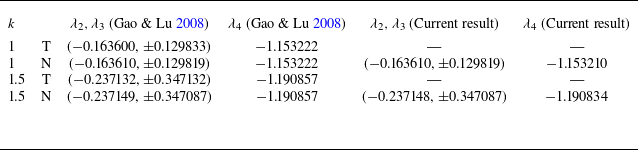
In the case where only periodic oscillations are considered ( $\gamma =0$ ), the numerical results are compared with those of Gao & Lu (Reference Gao and Lu2008) to validate consistency. In the absence of gravity, the results for $Re=0.5$ , $\chi =0$ , $Ca=0.05$ , $\beta =3$ , $M=10^{-3}$ and $\gamma =0$ are shown in table 2. The first four eigenvalues obtained under these parameters are $\lambda _{1}$ $\sim$ $\lambda _{4}$ . Here $\lambda _{1}$ corresponds to the trivial solution and is not shown. $\lambda _{2}$ and $\lambda _{3}$ are complex conjugates and $\lambda _{4}$ is real. It is observed that the current results agree well with the results from Gao & Lu (Reference Gao and Lu2008).

Table 2.

Comparison of theoretical (T) and numerical (N) results for $\lambda _{2}$ , $\lambda _{3}$ and $\lambda _{4}$ with $Re=0.5$ , $\chi =0$ , $Ca=0.05$ , $\beta =3$ , $M=10^{-3}$ and $\gamma =0$ .

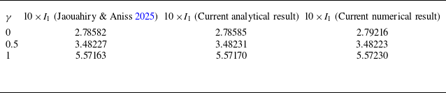
For the case of quasiperiodic oscillations in the absence of surfactants, our numerical results are compared with those presented by Jaouahiry & Aniss (Reference Jaouahiry and Aniss2025) to verify consistency. The results for fixed values of $\omega =\omega _{1}/\omega _{2}=1$ , $\chi =1$ , $Ca=0.05$ , $\beta =1$ and $M=0$ are shown in table 3. In their study, Jaouahiry & Aniss (Reference Jaouahiry and Aniss2025) reported an intermediate quantity associated with the eigenvalue computation, corresponding to $10\times I_{1}$ in the present study. Here, we provide the corresponding theoretical and numerical results for direct comparison. It is also observed that the current results agree well with the results from Jaouahiry & Aniss (Reference Jaouahiry and Aniss2025).

Table 3.

Comparison between analytical results at long wavelengths and numerical results with $\omega =\omega _{1}/\omega _{2}=1$ , $\chi =1$ , $Ca=0.05$ , $\beta =1$ and $M=0$ .

Figure 10.

Comparison of long-wavelength approximation results (dashed lines) and numerical results (solid lines) for $\beta =2$ , $Re=200$ , $\chi =1$ , $Ca=0.05$ , $M=10^{-2}$ and $\gamma =1$ . ( $a$ ) The real part of $\lambda$ for $\omega =\sqrt {37}$ . ( $b$ ) The real part of $\lambda$ for $\omega = {1}/{\sqrt {37}}$ .

In order to further verify the accuracy of the code and the correctness of the long-wavelength results, we compare the analytical solution of the long-wavelength limit obtained in § 3 with the current numerical results. According to (3.32), for $k\lt \lt 1$ , the eigenvalues dominating the flow stability are characterized by the Floquet parameter, $\lambda =\lambda _{0}+k\lambda _{1}+k^{2}\lambda _{2}+\ldots$ , where $\lambda _{0}=\lambda _{1}=0$ . Figure 10 shows the variation of $\lambda _{2}$ and that of the real part of $\lambda$ , namely $\lambda _{r}$ , as a function of $k$ for $\beta =2$ , $Re=200$ , $\chi =1$ , $Ca=0.05$ , $M=10^{-2}$ and $\gamma =1$ with different $\omega$ . For $\omega =\sqrt {37}$ , excellent agreement between numerical results and theoretical predictions is observed. Similarly, for $\omega =1/\sqrt {37}$ , a high level of consistency is also observed, particularly in the regime $k\lt 3\times 10^{-3}$ . In the presence of surfactant, two distinct growth rates are observed. However, since the numerical and theoretical results for both are in close agreement, only the results corresponding to one of the growth rates are presented here for brevity.

5. Finite-wavelength instability

Figure 11.

Stability characteristics in the presence of surfactants with $Ca=0.05$ , $\chi =1$ , $\omega =\sqrt {37}$ , $\gamma =1$ for different surfactant parameters $M=10^{-6}$ ( $a,b$ ), $M=10^{-3}$ ( $c,d$ ) and $M=10^{-2}$ ( $e,f$ ). Panels ( $a$ ), ( $c$ ) and ( $e$ ) represent the stability boundaries in the $(\beta ,Re_{c})$ -plane and panels ( $b$ ), ( $d$ ) and ( $f$ ) represent variation of the corresponding wavenumber $k_{c}$ with $\beta$ .

In this section, we will discuss the stability of quasiperiodic oscillation liquid film containing surfactants under arbitrary wavelength disturbance. The effects of modulation frequency and amplitude ratios are considered in long-wavelength analysis in § 3; therefore, they will not be discussed further here. Here we focus on the effect of surfactant concentration under arbitrary wavelength disturbance. Also, the presence or absence of gravity has an extremely limited effect on finite-wavelength stability, thus the case of no gravity is not discussed here. For comparison, we choose the same parameters as those in Or (Reference Or1997) and Jaouahiry & Aniss (Reference Jaouahiry and Aniss2025), i.e. $Ca=0.05$ , $\chi =1$ and the stability characteristics will be varying $\beta$ , $Re$ and $M$ .

Figure 11 illustrates the critical Reynolds number $Re_{c}$ and its corresponding critical wavenumber $k_{c}$ versus imposed frequency $\beta$ for three surfactant parameters ( $M=10^{-6}$ , $10^{-3}$ and $10^{-2}$ ) when $\omega =\sqrt {37}$ and $\gamma =1$ . The vertical dashed lines in the figure indicate the boundaries of the long-wavelength mode, while the slanted lines denote the boundaries of the finite-wavelength mode. Different from the long-wavelength results, when the Reynolds number exceeds a critical threshold, finite-wavelength instabilities emerge within regions where long-wavelength disturbances remain stable. As a result, regions dominated by long-wavelength modes and finite-wavelength appear alternately throughout the entire range of $\beta$ . The gaps in the $k_{c}-\beta$ curves correspond to the critical wavenumber $k_{c}=0$ in the long-wavelength instability mode.

For a lower surfactant concentration $M=10^{-6}$ in figures 11 $(a)$ and 11 $(b)$ , the flow instability is initially dominated by the long-wavelength mode as $\beta$ increases from zero. As $\beta$ increases to 2.57, the critical Reynolds number associated with the long-wavelength mode becomes equal to that of the finite-wavelength mode. In the subsequent range of oscillation frequencies $\beta$ , the finite-wavelength mode becomes dominant, with the corresponding disturbance wavenumber rapidly increasing from zero until the neutral stability curve intersects with the second U-shaped neutral curve. Following this intersection, the long-wavelength mode once again resumes dominance. When $\beta$ reaches 5.44, the dominant instability mode transitions once again from the long-wavelength to the finite-wavelength mode. However, the corresponding disturbance wavenumber is comparatively smaller than that observed in the previous finite-wavelength regime. Different from the case without surfactants in Jaouahiry & Aniss (Reference Jaouahiry and Aniss2025), the finite-wavelength instability boundary can be categorized into two distinct types. At lower frequencies, this boundary is associated with two neutral modes which belong to two complex-conjugate Floquet exponents with $\lambda _{i}\ne 0$ , implying that the corresponding neutral disturbances take the form of travelling waves. Moreover, another finite-wavelength stability boundary with higher wavenumbers can be identified. This boundary is associated with a single neutral mode whose Floquet exponent has a zero imaginary part, indicating that the disturbance takes the form of a standing-wave mode. The two types of finite-wavelength boundaries intersect at point $P_{1}$ in figure 11 $(a)$ , corresponding to the frequency parameter $\beta =6.1$ . Figure 11 $(b)$ further reveals that, relative to the case without surfactants, the critical wavenumber displays a marked non-monotonic trend, with a sharp discontinuity observed in the vicinity of the intersection point. A similar discontinuity of the wavenumber has also been observed by Phillips (Reference Phillips2001).

For higher surfactant concentrations of $M=10^{-3}$ and $M=10^{-2}$ in figure 11(c–f), the critical Reynolds numbers and critical wavenumbers overall follow a similar pattern of variation. However, with increasing surfactant concentration, the widths of the first and second U-shaped neutral stability curves are observed to decrease significantly (as clearly illustrated in the discussion of figure 7), while the frequency range associated with finite-wavelength instability becomes broader. Moreover, the location of the intersection point shifts towards the lower-frequency region as the surfactant concentration increases. It is particularly noteworthy that as the surfactant concentration increases from $10^{-6}$ to $10^{-3}$ , the intersection point $P_{2}$ migrates from the second finite-wavelength boundary to the first, indicating the significant influence of surfactant concentration on the instability characteristics. A comparative examination further demonstrates that, at elevated surfactant concentrations, the critical Reynolds number corresponding to a fixed frequency increases, thereby indicating a stabilizing effect of surfactants on the flow system.

Figure 12.

Stability characteristics in the presence of surfactants with $Ca=0.05$ , $\chi =1$ , $\omega =\sqrt {7}$ , $\gamma =1.5$ for different surfactant parameters $M=10^{-6}$ ( $a,b$ ), $M=10^{-3}$ ( $c,d$ ) and $M=10^{-2}$ ( $e,f$ ). Panels ( $a$ ), ( $c$ ) and ( $e$ ) represent the stability boundaries in the $(\beta ,Re_{c})$ -plane and panels ( $b$ ), ( $d$ ) and ( $f$ ) represent variation of the corresponding wavenumber $k_{c}$ with $\beta$ .

Figure 13.

Typical neutral curves in the $(k,Re)$ -plane with $Ca=0.05$ , $\chi =1$ , $\omega =\sqrt {37}$ , $\gamma =1$ for different surfactant parameters $M=10^{-6}$ ( $a$ ), $M=10^{-3}$ ( $b$ ) and $M=10^{-2}$ ( $c$ ). Each curve represents different values of $\beta$ around the intersection point in figure 11.

Figure 12 shows the critical Reynolds number $Re_{c}$ and its corresponding critical wavenumber $k_{c}$ versus imposed frequency $\beta$ under three different sets of surfactant parameters, following variations in the frequency ratio $\omega =\sqrt {7}$ and amplitude ratio $\gamma =1.5$ . Overall, the trend of the curves is generally consistent with that of figure 11, exhibiting the alternating dominance between long-wavelength and finite-wavelength modes. Finite-wavelength disturbances can still be classified into two distinct modes, corresponding to travelling-wave and standing-wave perturbations, respectively. The intersection points ( $P_{1}$ , $P_{2}$ and $P_{3}$ ) between these modes also exhibit distinct characteristics. As the surfactant concentration increases, the intersection points of the two different modes shift towards smaller values of $\beta$ , and potentially migrating from the second finite-wavelength boundary to the first. As a matter of fact, for other frequency ratios $\omega$ and amplitude ratios $\gamma$ , the variations of $Re_{c}$ and $k_{c}$ with $\beta$ exhibit trends essentially consistent with those shown in figures 11 and 12, and are therefore not repeated here.

Typical neutral curves in the $(k,Re)$ -plane with $Ca=0.05$ , $\chi =1$ , $\omega =\sqrt {37}$ , $\gamma =1$ for different surfactant parameters are shown in figure 13. The different curves in the figure correspond to different frequency values of $\beta$ , all of which are distributed in the vicinity of the intersection point identified in figure 11. For the lower surfactant concentration $M=10^{-6}$ , the three curves in figure 13 $(a)$ correspond to $\beta$ values of 6.0, 6.1 and 6.2, respectively. Notably, at $\beta =6.1$ , an intersection of the finite-wavelength branches is observed in figure 11( $a$ ). As shown in figure 13 $(a)$ , each neutral stability curve can be divided into left- and right-hand branches, each exhibiting a local minimum. When $\beta =6$ , the left-hand branch exhibits a lower local minimum compared with the right-hand branch. Consequently, the critical point of the flow corresponds to the lowest point on the left-hand branch, with the associated critical parameters given by $Re_{c}=847$ and $k_{c}=0.296$ . As $\beta$ increases, the entire neutral stability curve shifts upwards, with the left-hand branch rising more rapidly than the right-hand branch. When $\beta =6.1$ , the two local minima of the neutral stability curve become aligned horizontally, corresponding to a critical Reynolds number of $Re_{c}=1063$ . Under this condition, the flow exhibits two critical disturbance wavenumbers, $k_{c}=0.292$ and $k_{c}=0.376$ , which correspond to the intersection values observed at the wavenumber discontinuity in figure 11 $(b)$ . When $\beta$ increases to 6.2, the critical parameters of the flow correspond to the lowest point on the right-hand branch of the neutral stability curve. At higher surfactant concentrations $10^{-3}$ and $10^{-2}$ , the neutral stability curves corresponding to different $\beta$ values exhibit qualitatively similar distributions. A more detailed examination of the eigenvalue characteristics shows that the left-hand branch is governed by complex-conjugate eigenvalues, which implies that this branch is associated with a travelling-wave instability mode. While the right-hand branch corresponds to purely real eigenvalues, suggesting that the instability mode in this case takes the form of a standing-wave mode. In terms of the flow physics, we examine the response behaviour to imposed perturbations by considering the flow at $\beta = 6.2$ in figure 13 $(a)$ as an example. As the Reynolds number increases, the first instability mode to emerge is the standing-wave mode represented by the right-hand branch of the curve, since at $\beta = 6.2$ this mode possesses a lower critical Reynolds number and is therefore more readily excited. At the critical frequency, the perturbation mode in the flow transitions from a propagating mode to a standing mode, or conversely. With the change in disturbance modes, the energy distribution within the flow undergoes significant variations. Travelling waves may transfer energy downstream, while standing waves could lead to energy accumulation in localized regions, thereby affecting the flow stability and its control mechanisms. As shown in figure 11, while the critical Reynolds number varies continuously, the presence of a bimodal structure in the neutral stability curves leads to a discontinuous transition in the critical wavenumber. This phenomenon is attributed to the mode competition between travelling-wave and standing-wave instabilities. In fact, for other frequency ratios $\omega$ and amplitude ratios $\gamma$ , the typical neutral curves in the $(k,Re)$ -plane at different surfactant concentrations exhibit similar trends and are thus omitted, confirming the generality of the present conclusion.

6. Energy budget analysis

We derive the disturbance energy balance equation for a liquid film with insoluble surfactants under the quasiperiodic oscillation, which enables us to elucidate the growth mechanisms of disturbances across arbitrary wavenumbers $k$ . By decomposing the balance and examining the contribution of each term to energy conservation budget, the budget quantifies the pathways of energy transfer. The perturbation governing equations obtained in § 2.2 are

(6.1) \begin{align} \frac {2\beta ^{2}}{\textit{Re}}\frac {\partial u'}{\partial t} +U_{b}\frac {\partial u'}{\partial x} +v'\frac {\partial U_{b}}{\partial y} &=-\frac {\partial p'}{\partial x} +\frac {1}{{\textit{Re}}^{2}}{\nabla} ^{2}u', \end{align}

(6.2) \begin{align} \frac {2\beta ^{2}}{\textit{Re}}\frac {\partial v'}{\partial t} +U_{b}\frac {\partial v'}{\partial x} =-&\frac {\partial p'}{\partial y} +\frac {1}{{\textit{Re}}^{2}}{\nabla} ^{2}v'. \end{align}

Taking the inner product with velocity components and carrying out an area integral over one disturbance wavelength yields the spatially periodic energy balance equation

(6.3) \begin{equation} \mathrm{RKINE} = \mathrm{REYNS}+\mathrm{SURTE}+\mathrm{HYDPR}+\mathrm{SHEST}+\mathrm{DISSI}, \end{equation}

where

(6.4a) \begin{align} &\mathrm{RKINE}=\frac {2\beta ^{2}}{\textit{Re}} \int \biggl ( u'\frac {\partial u'}{\partial t} +v'\frac {\partial v'}{\partial t} \biggl ) {\rm d}\mathrm{S}{\rm d}t, \end{align}

(6.4b) \begin{align} &\mathrm{REYNS}=-\int u'v'\frac {\partial U_{b}}{\partial y}{\rm d}\mathrm{S}{\rm d}t , \end{align}

(6.4c) \begin{align} &\mathrm{SURTE}=\frac {1}{\textit{Ca}} \int v'\frac {\partial ^{2} \eta '}{\partial y}\bigg |_{y=0} {\rm d}x{\rm d}t, \end{align}

(6.4d) \begin{align} &\mathrm{HYDPR}=\int v'\eta '\frac {\partial p'}{\partial y}\bigg |_{y=0} {\rm d}x{\rm d}t, \end{align}

(6.4e) \begin{align} &\mathrm{SHEST}=\frac {1}{{\textit{Re}}^{2}}\int u' \biggl ( \frac {\partial u'}{\partial y} +\frac {\partial v'}{\partial x} \biggl ) \bigg |_{y=0}{\rm d}x{\rm d}t, \end{align}

(6.4f) \begin{align} &\mathrm{DISSI}=-\frac {1}{{\textit{Re}}^{2}} \int \bigg [ \biggl ( \frac {\partial u'}{\partial x} \biggl )^{2} +3\biggl (\frac {\partial v'}{\partial y} \biggl )^{2}+\biggl (\frac {\partial v'}{\partial x}+\frac {\partial u'}{\partial y} ^{2} \biggl )\bigg ]{\rm d}\mathrm{S}{\rm d}t. \end{align}

As noted by Morgan et al. (Reference Morgan, Davies and Thomas2021), each term in (6.3) has a clear physical interpretation regarding its contribution to the system’s energy budget, and all terms are time dependent and periodic. Positive terms correspond to the generation of energy, while negative terms denote energy being removed from the system. Disturbances are amplified when energy production exceeds dissipation in the system. The RKINE term on the left-hand side of (6.3) represents the temporal variation rate of the perturbation kinetic energy. A positive RKINE indicates that, when integrated over one oscillation period, the perturbation kinetic energy increases, signifying an unstable flow with growing disturbances. A negative RKINE indicates decay of the perturbation kinetic energy. The REYNS term represents the work done by the Reynolds stress over a single oscillation period. The SURTE term denotes the work done by surface tension over an oscillation period. Here HYDPR represents the work expended against the basic flow pressure gradient at the free surface. When SURTE and HYDPR are positive, energy is being converted from the potential energy of the deformed free surface into fluid kinetic energy. Here SHEST denotes the work done by the shear stress at the free surface. Here DISSI represents the energy dissipation over one oscillation period, which is always negative and acts as a suppressive function in the energy budget.

To reveal the physical mechanisms driving the long-wavelength and finite-wavelength instabilities, we analyse how each term in the perturbation energy budget contributes to the evolution of the perturbation kinetic energy under different parameter regimes. We select typical parameters $\beta =1$ and $Re=10$ for long-wavelength instability, and $\beta =3$ , $Re=80$ for finite-wavelength instability, under fixed conditions of surfactants concentration $M=10^{-6}$ , the frequency ratio $\omega =\sqrt {37}$ and the amplitude ratio $\gamma =1$ . Under these two parameter combinations, the numerical values of all terms in the perturbation energy equation for the unstable cases are summarized in tables 4 and 5. The relative error is defined as $\epsilon _{r}=\{\mathrm{RKINE}-(\mathrm{REYNS}+\mathrm{SURTE}+\mathrm{HYDPR}+\mathrm{SHEST}+\mathrm{DISSI})\}/\mathrm{RKINE}\times 100\,\%$ . It can be seen that the relative errors for all data points remain at a low level, ensuring the accuracy of the numerical computations.

Table 4.

Numerical results of the energy contribution of each term in (6.3) for long-wavelength instability as a function of wavenumber $k$ when $\beta = 1$ , $Re = 10$ and $M = 10^{-6}$ .

Table 5.

Numerical results of the energy contribution of each term in (6.3) for finite-wavelength instability as a function of wavenumber $k$ when $\beta = 3$ , $Re = 80$ and $M = 10^{-6}$ .

Regarding the pressure gradient term HYDPR, its sign is consistently opposite to that of RKINE, indicating that, whether the perturbation kinetic energy grows or decays, the free-surface pressure gradient acts to oppose that trend. The surface shear stress term SHEST is strictly positive, indicating that it continuously enhances the perturbation kinetic energy. By contrast, the dissipation term DISSI is invariably negative and acts to decay the perturbation kinetic energy. It is important to note that the magnitudes of SHEST and DISSI are comparable and significantly exceed those of the other terms in the equation. Thus, the competition between these two dominant terms is pivotal in determining the stability characteristics of the flow. For the long-wavelength instability, SHEST is consistently larger than the magnitude of DISSI, indicating that the energy input supplied by surface shear stress is sufficient to offset the losses due to dissipation. However, for the finite-wavelength instability, SHEST is smaller than the magnitude of DISSI, indicating that the work of the surface shear stress is insufficient to balance the dissipative loss of perturbation kinetic energy. Moreover, closer inspection shows that the Reynolds stress work term, REYNS, plays markedly different roles in the two instability modes. For the long-wavelength instability the magnitude of REYNS is negligible and its contribution is minimal, whereas as the wavenumber increases into the finite-wavelength range the magnitude of REYNS grows rapidly, ultimately supplying sufficient energy to counterbalance the dissipation and sustain the disturbance growth.

Figure 14.

The time-averaged rates of work done by each energy terms under different surfactant concentrations $M$ , when ( $a$ ) $\beta =1$ , $Re=10$ for long-wavelength instability and ( $b$ ) $\beta =3$ , $Re=80$ for finite-wavelength instability. The abbreviations RK, RE, SU, HY, SH-DI represent RKINE, REYNS, SURTE, HYDPR and the sum of SHEST and DISSI, respectively.

Figure 14 illustrates the influence of different surfactant concentrations on the terms of the perturbation kinetic energy equation in the cases of long-wavelength and finite-wavelength perturbations. Preliminary analysis showed that frequency ratios $\omega$ and amplitude ratios $\gamma$ exert weaker effects on the energy budget than surfactant concentrations. Hence, the present discussion concentrates on how surfactant concentration affects each energy term. For mechanistic clarity, the surface shear stress term SHEST and the dissipation term DISSI are combined and denoted as SH-DI $\ =\mathrm{SHEST}+\mathrm{DISSI}$ , which characterizes the net effect of surface stress work and dissipation. In the case of long-wavelength perturbations, shown in figure 14(a), both RKINE and SH–DI exhibit consistent trends across different surfactant concentrations and wavenumbers, while the magnitudes of the other terms in the equation are considerably smaller and thus insufficient to alter the overall energy balance, highlighting the dominant contribution of the surface shear stress. As the surfactant concentration increases, the amplitudes of all energy terms decrease, leading to a slower growth of disturbance kinetic energy, which manifests as a stabilizing effect on long-wavelength instability. For finite-wavelength perturbations shown in figure 14(b), when the surfactant concentration $M=10^{-6}$ , RKINE is positive across all examined wavenumbers, signifying instability. In this regime, the energy budget is then dominated by the Reynolds stress term REYNS, whose magnitude exceeds the net dissipation represented by SH–DI. With increasing surfactant concentration, RKINE changes from positive to negative, indicating a transition from instability to stability. Accompanying this transition, the surface tension work term SURTE changes from negative to positive with increasing magnitude, revealing a more significant role of surface tension in enhancing perturbation kinetic energy. Nevertheless, at higher surfactant concentrations, REYNS stays positive but its relative contribution diminishes, whereas the net dissipation SH–DI is enhanced, resulting in $\mathrm{RKINE}\lt 0$ . In summary, compared with the long-wavelength perturbations, REYNS consistently promotes the growth of perturbation kinetic energy under finite-wavelength perturbations, with a more pronounced impact. For the horizontally oscillating liquid film, long-wavelength instability is governed primarily by surface shear stress, while finite-wavelength instability involves both Reynolds stress and surface shear stress. Additionally, the influence of surface tension becomes more significant with increasing surfactant concentrations.