1 Introduction
In recent times, human exploitation of space has enormously increased, resulting in an increased number of flying pieces of debris or space junk which can collide with space stations, space shuttles and live satellites and may result in heavy damage. This increase in the amount with time of natural and man-made debris has posed a serious challenge to the safety of human activities in space, as well as for smooth operation of man-made satellites (Laurance & Brownlee Reference Laurance and Brownlee1986; Peter Reference Peter1988; Liou & Johnson Reference Liou and Johnson2006; Dov Reference Dov2020). A space debris orbits around Earth with an angular momentum such that the centrifugal force balances the Earth's gravitational force and maintains a constant altitude. For safe human activity in space, de-orbiting space junk is an emergent technological challenge. Due to the Earth's gravitational force, the natural orbit decay rate of a space debris is very small and, left to itself, space debris will take an enormous amount of time to re-enter into the Earth's atmosphere depending upon the current altitude of the space debris. An external drag force acting on space debris can decelerate/accelerate the debris and can result in the re-entry of debris into the Earth's atmosphere where it can burn out (Shan, Guo & Gill Reference Shan, Guo and Gill2015).
Several techniques have been proposed in the past to manoeuvre the re-entry of space debris into the Earth's atmosphere. For example, a ground based powerful laser pulse system can be used to ablate debris material. This will change the debris orbital velocity and make it possible for re-entry into the Earth's atmosphere where burn out can take place (Rubenchik, Fedoruk & Turitsyn Reference Rubenchik, Fedoruk and Turitsyn2014). A low divergence ion beam can be used for contactless removal of space junk by direct momentum transfer (Bombardelli & Peláez Reference Bombardelli and Peláez2011; Kitamura, Hayakawa & Kawamoto Reference Kitamura, Hayakawa and Kawamoto2014). Robotic arms and tether nets are potential methods to capture active space debris and de-orbit them (Castronuovo Reference Castronuovo2011; Shan, Guo & Gill Reference Shan, Guo and Gill2017). An electro-dynamic tether technology is investigated as it has an efficient orbital transfer system (Nishida et al. Reference Nishida, Kawamoto, Okawa, Terui and Kitamura2009).
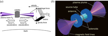
More recently, a magnetic nozzle plasma thruster with both ends open or a bi-directional plasma thruster for active removal of space debris has been suggested by Takahashi et al. (Reference Takahashi, Charles, Boswell and Ando2018b) and Takahashi (Reference Takahashi2019). Figure 1(a) shows the concept of space debris removal via direct momentum transfer of an ejected beam, using a bi-directional plasma thruster. Here, $F_{1}$ and $F_{2}$
 are the momentum fluxes ejected from two opposite ends of the device. A drag force $F_{1}$
 decelerates the space debris and helps it to re-enter into the Earth's atmosphere where it is burnt out (Goebel & Katz Reference Goebel and Katz2008). Figure 1(b) shows a magnetic nozzle with both ends open, forming a single thruster device where the momentum flux is controlled via a magnet coil current and neutral fuel flow rate. This electric propulsion device can be mounted on a satellite and can act as a debris remover or accelerate–decelerate the satellite by altering the magnetic field profile using the coil current. Takahashi et al. experimentally demonstrated that, for a symmetric magnetic field expansion profile at both ends of the radio frequency (RF) heating region, a net thrust is imparted at a plate suspended into the experimental chamber. Here, the suspended plate works as a dummy space debris. A net zero thrust is imparted on a flying satellite working with a symmetric magnetic field expansion bi-directional plasma thruster; i.e. $F_{1}=F_{2}$
 . For an asymmetric magnetic field expansion at both ends of the heating region, a net thrust at a satellite can be imparted in a particular direction depending upon the magnetic field profile; i.e. $F_{1}\neq F_{2}$
 . Hence, a bi-directional plasma thruster can have three working modes viz., a satellite acceleration mode, a deceleration mode and a debris removal mode by altering the magnet coil current.
(a) Working principle of a bi-directional plasma thruster while operating in space debris remover mode. (b) A single bi-directional plasma thruster where the momentum fluxes ejected at both ends are controlled by external operating nobes. (Picture credit: Kazunori Takahashi, Christine Charles, Rod W. Boswell & Akira Ando, Demonstrating a new technology for space debris removal using a bi-directional plasma thruster, Scientific Reports 8:14417 (2018), with approval of K. Takahashi.).

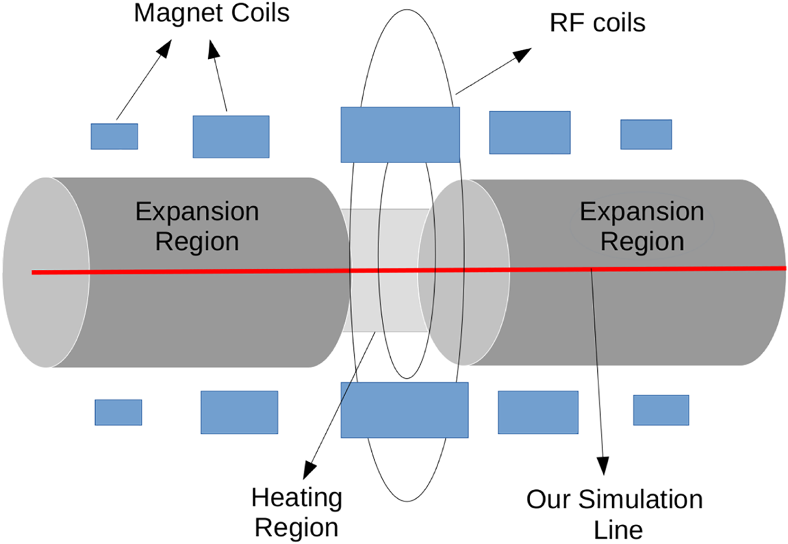
In this work, we have performed a set of numerical experiments for a doubly open-ended magnetic nozzle plasma thruster or a bi-directional plasma thruster using a standard particle in cell (PIC) simulation technique. Although this is an inherently three-dimensional problem, we have performed our simulations in one dimension, along the length of the nozzle's symmetric axis, as shown in figure 2. While averaging over two spatial directions (i.e. radial and angular directions), several physically relevant effects (e.g. $E \times B$ dynamics, radial transport; E, electric field and B, magnetic field) would naturally be neglected. To partially compensate, we have incorporated the effect of magnetic field expansion and compression on the plasma via a magnetic flux conservation model (Ebersohn, Sheehan & Gallimore Reference Ebersohn, Sheehan and Gallimore2015). We believe our reduced model can be useful in the understanding of experimental results for a bi-directional plasma thruster and to search the vast parameter space during optimization. In this work, variations in the directed ion beam velocity amplitude are scanned with a magnetic field expansion rate and neutral Ar gas density. A net thrust is generated for an asymmetric magnetic field configuration and qualitatively compared with recent experimental results for a bi-directional plasma thruster. To capture a more detailed picture of a bi-directional plasma thruster, a higher spatial dimensional code (e.g. 2D3V) may be required which can be expensive in terms of computational resources and time.
Schematic diagram of a two-open-ended magnetic nozzle where our simulation domain is the nozzle axis, which is shown by the red coloured line.

A 1D3V PIC Monte Carlo collision (PIC-MCC) (Hockney & Eastwood Reference Hockney and Eastwood1981; Chen Reference Chen1990; Jackson Reference Jackson1991; Birdsall & Langdon Reference Birdsall and Langdon1992; Cartwright, Verboncoeur & Birdsall Reference Cartwright, Verboncoeur and Birdsall2000) code, called EPPIC (Expanding Plasma PIC Solver) (Saini et al. Reference Saini, Pandey, Trivedi and Ganesh2018; Saini & Ganesh Reference Saini and Ganesh2020), is well benchmarked and used here to study the plasma dynamics in an expanding magnetic field plasma device such as the helicon plasma thruster (HPT) or a magnetic nozzle (Saini et al. Reference Saini, Pandey, Trivedi and Ganesh2018; Saini & Ganesh Reference Saini and Ganesh2020). The code resolves one spatial dimension, which is the direction of the nozzle axis and all three velocity dimensions. The geometrical forces acting on charged particles are incorporated and solved using the Boris particle pusher algorithm (Boris Reference Boris1970; Qin et al. Reference Qin, Zhang, Xiao, Liu, Sun and Tang2013; Ebersohn et al. Reference Ebersohn, Sheehan and Gallimore2015). We have assumed implicitly that electrons are magnetized and trapped inside a magnetic flux tube. A flux tube cross-sectional area (magnetic flux conservation model) is used to incorporate the effect of magnetic field compression and expansion on charged particles (Ebersohn et al. Reference Ebersohn, Sheehan and Gallimore2015).
In a HPT or magnetic nozzle, plasma expands from source region into an expansion region following strong guided magnetic field lines. Typically, in the plasma expansion region, particle density varies 1–2 orders in comparison with the source region. The change in density can be mimicked by a variation of the cross-sectional area of the magnetic flux tube. As plasma expands into the diverging magnetic field, particles following the magnetic field lines or plasma will get expanded to follow the magnetic flux surfaces. The cross-sectional area of the magnetic flux tube can be calculated if one uses the approximation that the radial contribution of the flux is negligible in comparison with the total flux. For known flux tube inlet cross-sectional area and magnetic field strength, the cross-sectional area can be calculated throughout the domain at any location along the $z$ -axis, i.e.

where $A_{1}$ and $A_{2}$
 are the cross-sectional areas of the magnetic flux tube at different axial locations. Here, $A_{2}$
 can be calculated if $B_{1}$
 , $B_{2}$
 and $A_{1}$
 are known, where $B_{1}$
 and $B_{2}$
 are magnetic field values at two different axial locations.
This cross-sectional area is then used in the Poisson equation to incorporate the axial density variation effect, which in turn helps to mimic the magnetic field compression and expansion effect on plasma particles.
A magnetic nozzle device or HPT is a cylindrical device. Inertial effects due to the coordinate system can be incorporated into the force equation as (Ebersohn et al. Reference Ebersohn, Sheehan and Gallimore2015; Saini & Ganesh Reference Saini and Ganesh2020)

where $\boldsymbol {v}=(v_{r},v_{\theta },v_{z})$ and $\boldsymbol {E}$
 and $\boldsymbol {B}$
 are the electric and magnetic fields, respectively, $r_{L}$
 is the particle Larmor radius, q is charge of the particle, m is mass of the particle and $\theta$
 is azimuthal direction in cylindrical co-ordinates. As the problem considered is non-relativistic, the electric field $\boldsymbol {E}$
 is independent of the particle velocities. Hence, we first solve (1.2) without the $\boldsymbol {E}$
 -term and include the same while computing the full equations of motion, as shown below.
Let us start with the Maxwell equation $\boldsymbol {\nabla } \boldsymbol {\cdot } \boldsymbol {B} =0$ , which can be written in simplified form using the approximation that magnetized particles are small current loops orbiting around magnetic field lines and $B_{z}$
 is assumed to be uniform over the Larmor radius $r_{L}$
 , resulting in

After substituting $B_{r}$ into (1.2) (without $\boldsymbol {E}$
 term), the simplified model equations are:


It is pertinent to note the following: (1.6) indicates that $v_{r}$ is a non-zero constant in our simulations, which implies that the magnetic field, $\boldsymbol {B}$
 , does not alter the radial velocity component. Also, it has been assumed implicitly that particles are in the frame of reference along the magnetic field lines. The force equations (now including the electric field) in the frame of the magnetic field lines are


where $s$ is defined as direction along the magnetic field line. The azimuthal velocity ($v_{\theta }$
 ) is the velocity perpendicular to the magnetic field line ($v_{\perp }$
 ). The forces (1.7) and (1.8) are solved using the Boris particle pusher algorithm. The initial half-push is performed with an electric field. This is followed by the magnetic field push and the final half-push is performed by the electric field. To solve the magnetic field force on the particles, the energy conservation principle is used because the work done by the magnetic field on charged particles is zero. Because of energy conservation, one can write

After simplification of the parallel velocity component, $v_{\parallel }$ at the $n+1$
 th time step can be written as

where $\zeta =({1}/{2B})({{{\rm d}}B}/{{{\rm d}}s})$ and $K$
 are constant over $\triangle t$
 (Appendix A).
An asymmetric inductive excitation scheme is used to energize the electrons (Meige, Boswell & Charles Reference Meige, Boswell and Charles2005; Ebersohn et al. Reference Ebersohn, Sheehan and Gallimore2015; Saini & Ganesh Reference Saini and Ganesh2020). An RF electric field $E_{y}$ of frequency $f={\omega }/{2 {\rm \pi}}=13.56$
 MHz is applied normal to the axial direction to heat the electrons. The $\hat {y}$
 -direction is in the $\hat {r}-\hat {\theta }$
 plane, which is perpendicular to the axial direction. The amplitude of this RF electric field is chosen to avoid overheating of the electrons. Hence, the RF current density $J_{0}$
 is used as the control parameter for the RF electric field amplitude $E_{y}$
 . The total current density in the source region is


where $\varGamma _{e,y}$ is the electron flux along the $y$
 -axis. Here, $\varGamma _{e,y}$
 is

using Maxwell's equations, which results in

where $J_{0}$ is the RF current density, $L_{source}$
 is the length of the heating region and $N_{\sigma }$
 is the weight of a macro-particle.
An energetic electron collides with a neutral Ar fuel gas atom and further generates an electron–ion pair via ionization collision (Verboncoeur et al. Reference Verboncoeur, Alves, Vahedi and Birdsall1993; Vahedi & Surendra Reference Vahedi and Surendra1995; Frignani & Grasso Reference Frignani and Grasso2006). These particles evolve in time, inducing further ionization, or remain as bulk species and, after a sufficiently large simulation time, the system attains a steady state. Once steady state is achieved, desired quantities are stored to understand the late time behaviour of the system. It is important to note that, in our PIC-MCC simulations, electron–neutral and ion–neutral collisions comprising of elastic, ionization and excitation collisions as well as charge exchange collisions have been included, whereas electron–electron and electron–ion and ion–ion collisions have been neglected. For low energy electrons, scattering is more isotropic and energetic electrons witness forward scattering (small scattering angles). Here, we have used direct analytical formulae for argon collision cross-sections following the strategy used in the XOOPIC code (Frignani & Grasso Reference Frignani and Grasso2006). These formulae are known to accurately reproduce a database for argon collision cross-sections and are, at the same time, easy to implement.
The spatial magnetic field profile used in our simulations is

where $L$ is the total axial length of the system, $l_{b}$
 is a control parameter for the magnetic field expansion rate and $B_{0}$
 is the magnetic field amplitude. We have chosen $z_{0}=0.6\times L$
 on the right-hand side of the heating region and $z_{0}=0.4\times L$
 on the left-hand side of the heating region. With decreasing $l_{b}$
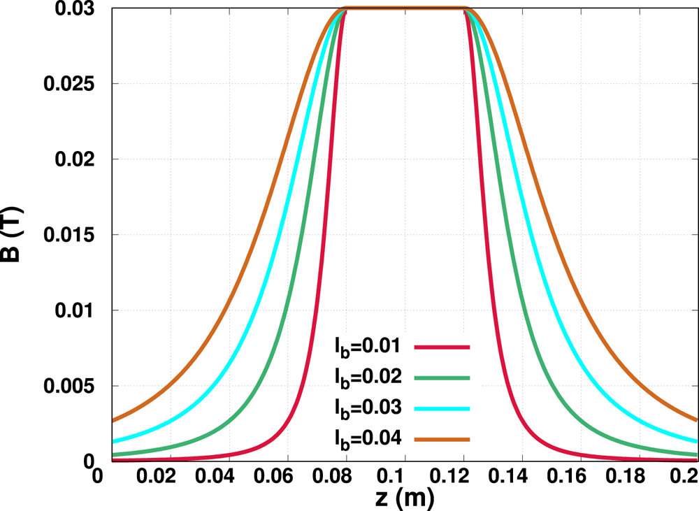
 , the magnetic field gradient increases in the expansion chamber and this results in rapid expansion of plasma charged particles in an experimental chamber (Baalrud et al. Reference Baalrud, Lafleur, Boswell and Charles2011; Ebersohn et al. Reference Ebersohn, Sheehan and Gallimore2015). Figure 3 shows the spatial magnetic field profile for different $l_{b}$
 values having a symmetric magnetic field expansion profile on both sides of the plasma heating region. For the magnetic field strength and electron temperatures considered in this work, a typical average Larmor radius is approximately $1.9 \times 10^{-4}$
 m. Here, in our simulation, electrons are regarded as magnetized and the strength of the bulk potential depends upon the magnetic field gradient in the expansion region.
The spatial magnetic field profile with different $l_{b}$ for a symmetric magnetic field expansion. Here, the heating region starts from $z=0.08$
 and ends at $z=0.12$
 .

This model does not include the neutral flow dynamics, although it is a critical parameter in a working device (Takao & Takahashi Reference Takao and Takahashi2015; Takahashi, Takao & Ando Reference Takahashi, Takao and Ando2016; Takahashi Reference Takahashi2021). Here, we also do not include the plasma plume interaction with the spacecraft body and charge particle detachment from the magnetic field lines, which are the critical phenomena for thruster performance. As indicated earlier, our 1D3V PIC-MCC solver is written in a Cartesian geometry. The HPT is a cylindrical device and geometrical forces (inertial forces) are included indirectly using model equations (Delzanno & Camporeale Reference Delzanno and Camporeale2013; Ebersohn et al. Reference Ebersohn, Sheehan, Gallimore and Shebalin2017). It may be noted that, in the magnetic field frame of reference, while we need only two velocity components, namely $v_{\perp }$ and $v_\parallel$
 , 3 velocity components are required for calculating the particle collision dynamics. We have used the energy conservation principle to calculate the magnetic field force on the charged particle and any change in $v_{\parallel }$
 would be reflected in both perpendicular directions, $v_{\perp }=\sqrt {v_{x}^{2}+v_{y}^{2}}$
 .
2 Numerical simulation
To start with, the simulation domain is seeded with 1 eV Maxwellian stray electrons and ions which are then energized using the inductive heating scheme to obtain plasma discharge. We have performed two different sets of numerical simulations, one having a symmetric magnetic field expansion and the other having an asymmetric magnetic field expansion in real space for a bi-directional plasma thruster. For the symmetric magnetic field expansion case, $l_{b}$ is kept same on both sides of the heating region. In the asymmetric magnetic field expansion case, $l_{b}$
 is kept constant on one side of the heating region and is varied on the other side to create an asymmetry in the B-field expansion rate. In our simulation, the heating region starts from $0.4 \times L$
 and ends at $0.6\times L$
 . Consequently, for our system size $L=0.2$
 m, the heating region is situated at the centre of the simulation domain having a length of 0.04 m. The length of the expansion chamber is 0.08 m on both sides.
Throughout the numerical simulation, both ends of the simulation domain are grounded, i.e. we use metal boundary condition. Particles crossing the end walls are removed from the simulation domain. Although on an operational bi-directional thruster both ends will be open, in general, to reduce the substantial computational cost, metal boundary conditions are used in PIC simulations.
To further justify the use of a Dirichlet boundary condition, let us note that, in a terrestrial laboratory experimental system, metallic boundaries are far away. Also, in a realistic working device, where a bi-directional thruster is mounted on a spacecraft, both ends will be open. Typically, the length of a terrestrial experimental device is several times (say 5 to 6 times at least) larger than our typical simulation length. Hence, setting up and running simulations for such experimental device length scales is computationally expensive. However, recently, we have shown that, with increasing simulation length, the plasma sheath electric field become more localized close to the walls and it was observed that the bulk ion beam physics and the plasma sheath physics can be clearly delineated from each other (Saini & Ganesh Reference Saini and Ganesh2020). In the present work, our simulation length is sufficiently large to delineate the bulk plasma effect and the sheath effect. Here, the length of our plasma simulation domain is around 280$\bar {\lambda }_{D}$ , where $\bar {\lambda }_{D}$
 is the average plasma Debye length. Generally, the length of a conventional plasma sheath at the walls is 5–10$\bar {\lambda }_{D}$
 . In a HPT, ions are accelerated due to a double layer potential formed in the bulk plasma and, indirectly, the source of this potential drop in the bulk plasma is the electron energy (Sheehan et al. Reference Sheehan, Longmier, Bering, Olsen, Squire, Ballenger, Carter, Cassady, Chang Diaz and Glover2014). In an expanding magnetic plasma thruster, the radial electron pressure is converted into axial momentum flux and the electron temperature is reduced in the axial direction due to the loss of internal energy, while ions get accelerated. Boundary conditions on both sides do affect the ion beam dynamics (Chen Reference Chen2006; Takahashi, Shida & Fujiwara Reference Takahashi, Shida and Fujiwara2010; Boswell et al. Reference Boswell, Takahashi, Charles and Kaganovich2015; Takahashi et al. Reference Takahashi, Charles, Boswell and Ando2018a, Reference Takahashi, Charles, Boswell and Ando2020), however, we have chosen a simulation length sufficiently large so that the sheath electric field effect at the walls is sufficiently localized close to the walls and does not seriously influence the physics of bulk ion acceleration. This approach is often used in numerical simulation to cut down the overall simulation time (Meige et al. Reference Meige, Boswell and Charles2005; Ebersohn et al. Reference Ebersohn, Sheehan and Gallimore2015).
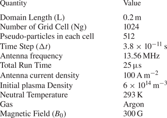
The results presented here are averaged over the last few RF cycles. A set of input parameters for our simulation results is given in table 1 (Meige et al. Reference Meige, Boswell and Charles2005; Saini & Ganesh Reference Saini and Ganesh2020).
Standard Simulation Input Parameters for a Bi-directional plasma thruster.

2.1 Symmetric magnetic field expansion
As discussed above, for the symmetric magnetic field expansion case, the magnetic field expansion rate $l_{b}$ is kept the same on both sides of the heating region. In principle, this kind of bi-directional thruster mounted on a spacecraft imparts zero net thrust on the device and can be used to impart a non-zero thrust on debris flying in space. Thus, a symmetric bi-directional plasma thruster can decelerate debris and push it into the Earth's atmosphere, where it will be burnt. Therefore, this kind of magnetic field configuration in a bi-directional plasma thruster can be used for debris removal in space. Here, a detailed numerical simulation study is performed for the symmetric magnetic field expansion case, where, in the first set, the neutral fuel, Ar, gas density is kept constant while varying the $l_{b}$
 and, in the second set, the $l_{b}$
 value is kept constant while varying the neutral fuel Ar gas density.
2.1.1 The $l_{b}$ variation at fixed Ar fuel density

In the first case of symmetric magnetic field expansion, we have used four different values of $l_{b}$ , namely $l_{b}=0.01$
 , $0.02$
 , $0.03$
 and $0.04$
 while the neutral fuel Ar gas density is fixed at 1.23 mTorr (Ebersohn et al. Reference Ebersohn, Sheehan and Gallimore2015). As already discussed, the magnetic field expansion rate increases with a decreasing value of $l_{b}$
 and this results in rapid expansion of plasma charged particles in the experimental chamber.
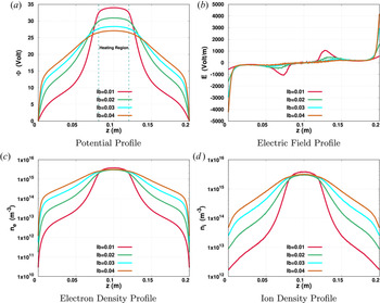
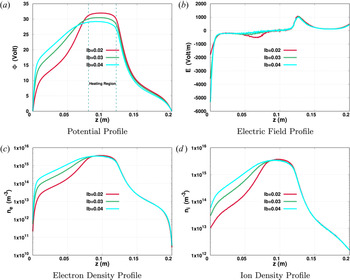
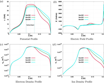
In a bi-directional plasma thruster having a symmetric magnetic field expansion rate on both sides of the heating region, the plasma expansion dynamics is investigated with varying $l_{b}$ . In figure 4, plasma field quantities and particle densities are shown with varying magnitudes for a symmetric magnetic field expansion rate. Figure 4(a) shows that the peak value of the bulk plasma potential decreases as $l_{b}$
 increases. A rapid fall in the electric potential is seen in the boundary sheath region as $l_{b}$
 increases. While the plasma expands into a diverging magnetic field, electrons lag behind the ions due to the large mass difference and a potential difference is generated in the bulk plasma. This bulk plasma potential difference is favoured in the presence of an expanding magnetic field. In our simulation, electrons are magnetized and a magnetic dipole force acts along the axial direction. This force increases with the divergence of the magnetic field and generates a potential drop in the bulk plasma. A potential drop is the signature of a plasma double layer which self-consistently accelerates the ions. As the magnetic field divergence increases, the potential drop in the bulk plasma rapidly increases and generates a large electric field in the bulk plasma. In figures 4(c) and 4(d), electron and ion density spatial profiles are shown in a logarithmic scale. The particle densities drop by 1–2 orders when moving from the heating region to expansion regions.
Plasma field and particle density spatial profile with different $l_{b}$ values for a symmetric magnetic field expansion, where Ar neutral pressure is fixed at 1.23 mTorr. The heating region is situated between the dashed dark-cyan lines, as shown in (a).

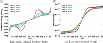
Figure 5 shows a plot of the ion mean velocity and flow rate spatial profile for a symmetric magnetic field expansion on both sides of the plasma heating region. The ion mean velocity reduces with increasing $l_{b}$ , which is quite obvious because the electric field strength in the bulk plasma reduces as we increase the $l_{b}$
 . Here, the ion flow rate is defined by $n_{i} \bar v_{iz} A$
 , where $n_{i}$
 is the ion number density, $\bar v_{iz}$
 is the ion mean velocity in the $z$
 -direction and $A$
 is the magnetic flux tube cross-sectional area. Figure 5(b) shows a constant slope for the ion flow rate in the plasma heating region. This implies a constant source rate in the plasma heating region. In the expansion region, the ion flow rate is nearly constant because there are very few new particle generation events. The ion flow rate reduces with an increasing value of $l_{b}$
 because a higher $l_{b}$
 value results in a lower ion mean velocity.
Ion mean velocity and flow rate spatial profile with different $l_{b}$ values for a symmetric magnetic field expansion, where the Ar neutral pressure is fixed at 1.23 mTorr.

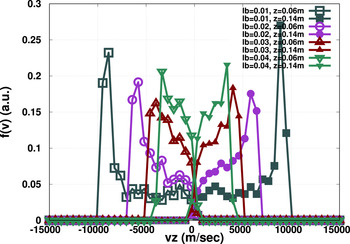
In figure 6, the ion velocity distribution function at two symmetric spatial locations, $z=0.06$ and $z=0.14$
 m, with respect to heating region, is shown for the symmetric magnetic field expansion case. While the plasma expands into a diverging magnetic field, an electric field is generated in the bulk plasma and accelerates the charged particles. The strength of this electric field depends on the magnetic field expansion rate. For $l_{b}=0.01$
 , which is the fastest rate of magnetic field expansion in our simulation, a directed ion beam having a velocity of approximately $9000\,{\rm m}\,{\rm s}^{-1}$
 is generated. The ion beam velocity reduces as $l_{b}$
 increases and, for $l_{b}=0.04$
 , the ion beam shows a shifted Maxwellian velocity distribution. Broadening in the ion velocity distribution function is due to ion–neutral charge exchange collisions and electron-neutral ionization.
Ion velocity distribution function at two symmetric spatial locations, $z=0.06$ and $z=0.14$
 m, with respect to the heating region for a symmetric magnetic field expansion. Here, the Ar neutral pressure is fixed at 1.23 mTorr.

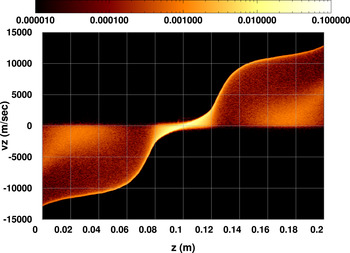
Figure 7 shows the ion phase space plot for symmetric magnetic field expansion for both sides of the plasma heating region having $l_{b}=0.01$ . It shows that the accelerated ion beams, in opposite directions, have identical velocity amplitudes right after the plasma heating region. As we have already discussed, the simulation length is chosen sufficiently large to delineate the directed ion beam from the sheath accelerated ions and minimize the effect of the sheath electric field on the bulk plasma dynamics. Here, our plasma is weakly collisional and most of the collision events occur in the plasma heating region. On both sides of the plasma heating region very few collision events occur, and a small opposite velocity ion population can be seen in the plasma expansion region.
For a symmetric magnetic field plasma expansion, an instantaneous ion phase space plot at $t=t_{end}$ , where $l_{b}=0.01$
 is chosen on both sides of the heating region and the Ar neutral pressure is fixed at 1.23 mTorr. The colour map represents the ion density in phase space.

2.1.2 The Ar fuel density variation at fixed $l_{b}$

In the second case of symmetric magnetic field expansion, we have used four different values of the neutral fuel Ar gas density, 1, 2, 5 and 10 mTorr while keeping $l_{b}=0.02$ throughout this simulation set. Here, the rest of the input parameters are identical to those previously used.
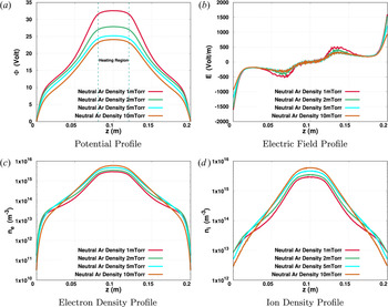
Here, a symmetric bi-directional plasma thruster is investigated with varying neutral Ar gas density. As shown in figure 8, the peak value of the bulk plasma potential and the electric field decrease as we increase the neutral Ar density. With increasing neutral density, charged particle collisions with neutral Ar atoms increase and the mean free path of charged particles reduces. High neutral Ar density works as a barrier in the expansion of charged particles and results in a lower bulk plasma potential. Figures 8(c) and 8(d) shows the electron and ion spatial density profiles. The charged particle density increases with Ar neutral density because of increasing collision probability.
Plasma field and particle density spatial profile with different Ar neutral pressures, where the symmetric magnetic field expansion rate $l_{b}$ is fixed at 0.02. The heating region is situated between the dashed dark-cyan lines, as shown in (a).

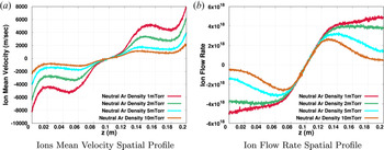
Figure 9 shows the ion mean velocity and flow rate spatial profile with varying neutral Ar density. The strength of the electric field in the bulk plasma reduces with increasing neutral Ar pressure and results in a lower ion mean velocity in the expansion region. An ion flow rate spatial profile with varying neutral pressure is shown in figure 9(b). The ion flow rate in the expansion region reduces with increasing neutral Ar fuel gas density. For the 5 and 10 mTorr cases, the ion flow rate shows a small dip in the expansion region because, for these cases, the system does not show a good convergence even at $t=25\,\mathrm {\mu }$ s.
Ion mean velocity and flow rate spatial profile with different Ar neutral pressures for a symmetric bi-directional B-field thruster, where the magnetic field expansion rate $l_{b}$ is fixed at 0.02.

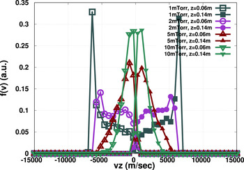
In figure 10, an ion velocity distribution is shown with varying Ar neutral pressure. For 1 mTorr neutral pressure, the ion velocity distribution function shows that the directed ion beam speed is around 6000 m s$^{-1}$ . As discussed above, ion acceleration reduces with increasing Ar neutral pressure and this is well reflected in the ion velocity distribution function plot. For 5 and 10 mTorr neutral pressures, the ion velocity distribution function shows a shifted Maxwellian behaviour. The ion velocity distribution function is shown at two different symmetric locations, $z=0.06$
 and $z=0.14$
 m, with respect to the heating region and, as expected, the velocity distribution functions are near mirror images of each other. Thus, a symmetric bi-directional plasma thruster imparts zero net thrust on a working device.
Ion velocity distribution function at two symmetric spatial locations, $z=0.06$ and $z=0.14$
 m, with respect to the heating region for a symmetric magnetic field expansion. Here, $l_{b}=0.02$
 is kept constant.

For the symmetric bi-directional thruster simulation, the potential and the particle density show symmetric behaviours on both sides of the heating region, which is expected. The directed ion beam velocity reduces with increasing $l_{b}$ value. As shown in the above simulation results, increasing the Ar neutral density reduces the directed ion beam velocity. To impart maximum thrust on space debris, the neutral gas density number and magnetic field expansion rate should be optimized for a spacecraft mounted bi-directional thruster (Takahashi et al. Reference Takahashi, Charles, Boswell and Ando2018b).
As discussed above, symmetric magnetic field expansion in a bi-directional plasma thruster can be used for space debris removal while imparting a net zero thrust on the working satellite or thruster. This thruster device, simultaneously, can be used as a space debris remover and to drive the live satellite by introducing an asymmetric magnetic field expansion on both sides of the heating region. A detailed study of an asymmetric magnetic field expansion case is given in the next section.
2.2 Asymmetric magnetic field expansion
The spatial magnetic field asymmetry in a bi-directional plasma thruster can produce a net momentum flux in a particular direction. This configuration, simultaneously, can be used in space debris removal and to control the live satellite velocity. This kind of bi-directional plasma thruster can be mounted on a spacecraft and can be used to accelerate or decelerate the spacecraft depending upon the magnetic field configuration.
In the asymmetric magnetic field expansion case, $l_{b}$ is kept constant at one side of the heating region and is varied on the other side. Two sets of numerical simulations have been performed for an asymmetric magnetic field expansion case. In the first set, $l_{b}$
 is kept constant on right-hand side of the heating region and is varied on left-hand side to generate an asymmetry in the magnetic field expansion. In the second set, the left and right side $l_{b}$
 values are swapped.
In figure 11, plasma field quantities and particle densities are shown having fixed $l_{b}=0.01$ on right-hand side, which parameter varies on the left-hand side. An asymmetry is generated in both plasma fields and particles densities due to different magnetic field expansion rates at the ends of the heating region. Additionally, for an asymmetric magnetic field expansion case the potential gradient in the expansion region reduces with increasing $l_{b}$
 and results in a lower electric field in the bulk plasma, as shown in figure 11(b). In figures 11(c) and 11(d), electron and ion density spatial profiles are shown, respectively. The particle density shows a large drop in the expansion region with increasing magnetic field expansion rate. For the second set of asymmetric magnetic field expansion cases, $l_{b}$
 is kept constant on the left-hand side and varies on the right-hand side. Other simulation parameters are kept constant. Figure 12 shows the plasma field and particle density spatial profiles and, as expected, they are mirror images of those shown in figure 11.
Plasma field and particle density spatial profile with different values of $l_{b}$ for an asymmetric magnetic field expansion, where the Ar neutral pressure is fixed at 1.23 mTorr. Here, $l_{b}=0.01$
 is kept constant on the right-hand side of the heating region. The heating region is situated between the dashed dark-cyan lines, as shown in (a).

Plasma field and particle density spatial profile with different values of $l_{b}$ for an asymmetric magnetic field expansion, where the Ar neutral pressure is fixed at 1.23 mTorr. Here, $l_{b}=0.01$
 is kept constant on the left-hand side of the heating region. The heating region is situated between the dashed dark-cyan lines, as shown in (a).

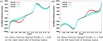
Figure 13 shows the ion mean velocity spatial profile for an asymmetric magnetic field expansion case. As plasma expands in a diverging magnetic field, an electric field is generated in the bulk plasma and accelerates ions. The accelerated ions result in a directed ion beam. The ion mean velocity in the expansion region drops with increasing $l_{b}$ because the electric field strength in the bulk plasma reduces as $l_{b}$
 increases. As expected, figures 13(a) and 13(b) are mirror image of each other.
Ion mean velocity spatial profile with different values of $l_{b}$ for an asymmetric magnetic field expansion, where the Ar neutral pressure is fixed at 1.23 mTorr.

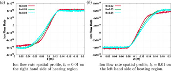
Figure 14 shows the ion flow rate spatial profile for an asymmetric magnetic field expansion case. The ion flow rate spatial profile shows a constant slope in the plasma heating region and implies that $nvA\rvert _{1}^{2}={\rm constant}$ . This shows a constant particle source term in the plasma heating region. On both sides of the plasma heating region, the ion flow rate is nearly constant because there are very few new particle generation events and there is no extra source of energy in the plasm expansion region.
Ion flow rate spatial profile with different values of $l_{b}$ for an asymmetric magnetic field expansion, where the Ar neutral pressure is fixed at 1.23 mTorr.

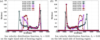
Figure 15 shows an ion velocity distribution function at two different axial locations with varying $l_{b}$ . In figure 15(a), $l_{b}=0.01$
 is kept constant on the right-hand side of the heating region and varies on the left-hand side. In the asymmetric magnetic field expansion case, the directed ion beam has a velocity of approximately $9000\,{\rm m}\,{\rm s}^{-1}$
 at $z=0.14$
 and at $z=0.06$
 m the directed ion beam velocity reduces with increasing $lb$
 . For $l_{b}=0.04$
 , the ion beam shows a shifted Maxwellian kind of distribution at $z=0.06$
 m. This magnetic field configuration can be used to generate thrust in a particular direction because the directed beam velocity is different on both sides of the heating region at a symmetric spatial location. Broadening in the ion velocity distribution is due to ion–neutral charge exchange collisions.
Ion velocity distribution function at two symmetric spatial locations, $z=0.06$ and $z=0.14$
 m, with respect to the heating region. For an asymmetric magnetic field expansion case, $l_{b}$
 is kept constant on one side of heating region and varies on the other side. Here, the Ar neutral pressure is fixed at 1.23 mTorr.

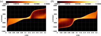
In the following, we have compared the instantaneous ion phase space at $t=25\,\mathrm {\mu }$ s for asymmetric magnetic field expansion cases. In figure 16(a), we have chosen $l_{b}=0.01$
 on the right of the heating region and $l_{b}=0.04$
 on the left side of the heating region to introduce an asymmetric B-field expansion. A directed ion beam is seen on the right of the heating region where the magnetic field expansion rate is high. Although ions get accelerated on the left-hand side of the heating region where $l_{b}=0.04$
 , the amplitude of the directed beam is small in comparison with the right. Thus, this configuration produces non-zero net thrust in a particular direction to control the satellite speed. In figure 16(b), $l_{b}$
 values are swapped on both sides of the heating region and, as expected, this is mirror image of figure 16(a).
Ion phase space plot for an asymmetric bi-directional plasma thruster. (a) Left-hand side $l_{b}=0.04$ and right-hand side $l_{b}=0.01$
 . (b) Left-hand side $l_{b}=0.01$
 and right-hand side $l_{b}=0.04$
 . Here, the Ar neutral pressure is fixed at 1.23 mTorr. Colour map represents the ion density in phase space.

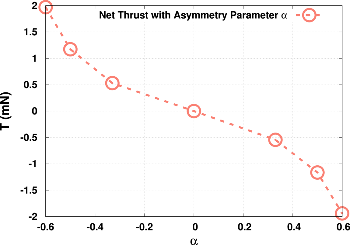
Figure 17 shows the net ion thrust in a particular direction with an asymmetry parameter $\alpha$ . Here, we have defined $\alpha = {(l_{b,right}-l_{b,left})}/{(l_{b,right}+l_{b,left})}$
 , where $l_{b,left}$
 and $l_{b,right}$
 are the plasma expansion rates on the left and right sides of the heating region, respectively. Here, thrust is defined as, $T= \dot m v_{exh}$
 , where $\dot m$
 (ion flow rate $\times$
 Ar atomic mass) is the ion mass flow rate and $v_{exh}$
 (corresponds to $z$
 component of the ion velocity, see figure 15) is the ion exhaust velocity at the thrust measurement spatial location. For $\alpha =0$
 , the net ion thrust is zero, which is a symmetric case and this type of magnetic field configuration can be used to decelerate flying space debris. With an increasing asymmetry parameter $\alpha$
 , the net ion thrust in a particular direction increases. For $\alpha =\pm 0.6$
 , the maximum ion thrust is achieved, having an amplitude of nearly 2 mN. Here, a positive thrust value indicates a net force on the right-hand side and a negative value indicates a net force on the left-hand side. In a real working device, both the direction and amplitude of the net ion thrust are controlled by a magnetic coil current and the fuel gas flow rate. As already discussed, we started with the strong approximation that, in our simulation, the neutral fuel gas Ar does not have a flow velocity. This approximation governs the ion flow rate and the actual magnitude of the thrust may change.
Net ion thrust in a particular direction with an asymmetric parameter $\alpha$ , where the Ar neutral pressure is fixed at 1.23 mTorr. Here, we define $\alpha = {(l_{b,right}-l_{b,left})}/{(l_{b,right}+l_{b,left})}$
 , where $l_{b,left}$
 and $l_{b,right}$
 are plasma expansion rates on the left and right sides of the heating region, respectively.

However, the net thrust in a HPT depends both on the dynamic ion momentum flux and the electron pressure term. In our model, we have assumed that magnetized electrons may have an excursion of approximately a Larmor radius and the cross-sectional area is used to incorporate the plasma expansion dynamics without explicitly including the radial direction and hence the radial dynamics. To include the electron pressure term in the net thrust calculation, the radial dynamics should be explicitly incorporated in the simulation; for example, we should take into account the electron azimuthal current due to electron diamagnetic drift (Fruchtman Reference Fruchtman2006; Takahashi et al. Reference Takahashi, Lafleur, Charles, Alexander and Boswell2011; Takahashi, Charles & Boswell Reference Takahashi, Charles and Boswell2013; Takahashi, Sugawara & Ando Reference Takahashi, Sugawara and Ando2020). This will require at the least, a 2D $RZ$ PIC-MCC code. In a one-dimensional simulation, the paraxial approximation is also used to calculate the electron pressure contribution to the net thrust (Takahashi et al. Reference Takahashi, Charles and Boswell2013). Thus, here, our thrust estimates are to be regarded as the lower bounds to the net thrust.
Takahashi et al. (Reference Takahashi, Charles, Boswell and Ando2018b) have investigated the effect of magnetic field strength and gradient on the net thrust produced in a bi-directional plasma thruster, by varying the solenoid current in the external coils. Our results shown in figure 17 of net ion thrust as a function of magnetic field asymmetry parameter $\alpha$ , may be compared qualitatively with the net thrust shown in figure 4 of Takahashi et al. (Reference Takahashi, Charles, Boswell and Ando2018b). Such a comparison shows remarkable qualitative similarity in spite of the absence of neutral particle flow in our model.
An asymmetric magnetic field configuration produces ion beams having different directed velocities in opposite directions at two symmetric locations on both sides of the heating region and results in a net thrust in a particular direction. This can be simultaneously used as a satellite accelerator–decelerator and debris remover in space. By changing coil current, which controls the magnetic field strength and gradient in a working device, the spacecraft speed can be controlled and one can alter its direction of motion also.
3 Summary and conclusions
In recent years, space junk or debris has become a serious challenge for the smooth operation of commercial satellites and space stations. Takahashi et al. (Reference Takahashi, Charles, Boswell and Ando2018b) proposed a bi-directional plasma thruster, where a directed ion beam can impart a net force in the opposite direction to de-orbit space debris. It is shown experimentally in a terrestrial laboratory that, depending upon the magnetic field spatial configuration, a device can operate in three modes; a satellite acceleration mode, a deceleration mode and a debris remover mode. A reduced one-dimensional model is developed to capture important aspects of a doubly open-ended diverging magnetic field plasma thruster.
For a symmetric magnetic field profile at both ends of the heating region, the plasma field and particle density profiles are symmetric, which is expected. The bulk plasma potential and electric field reduce with increasing $l_{b}$ values. We have observed a maximum speed for a directed ion beam of approximately 9000 m s$^{-1}$
 for $l_{b}=0.01$
 with the neutral Ar density fixed at 1.23 mTorr.
In experiments (Takahashi et al. Reference Takahashi, Charles, Boswell and Ando2018b), the neutral Ar density can be controlled by the flow rate at the fuel gas inlets. To capture the effect of the neutral density, we have used different values of neutral Ar gas density in our simulation without introducing a directed flow. The higher neutral particle density works as a barrier for plasma expansion in an experimental chamber and results in lower bulk plasma potential and electric field. For a $1$ mTorr neutral Ar density, we have observed a directed ion beam having a velocity of approximately $6000\,{\rm m}\,{\rm s}^{-1}$
 with $l_{b}$
 fixed at $0.02$
 and the amplitude reduces with increasing fuel density.
Our simulations presented here show that an asymmetric magnetic field configuration at both ends of the heating region can produce a net thrust in a particular direction depending upon the magnetic field spatial profile, demonstrating unambiguously that a bi-directional plasma thruster operational mode can be switched by changing the magnet coil current. In this configuration, for the parameters considered here, the maximum value of the net ion thrust, in a particular direction, is approximately 2 mN with $l_{b}=0.01$ on the right-hand side and $l_{b}=0.04$
 on the left-hand side of the heating region. The net ion thrust reduces with decreasing magnetic field gradient in the expansion chamber.
As discussed above, the neutral flow rate is a crucial parameter which controls the net thrust. The spatial neutral gas density profile would change net thrust numbers to some extent (Takao & Takahashi Reference Takao and Takahashi2015; Takahashi et al. Reference Takahashi, Takao and Ando2016; Takahashi Reference Takahashi2021). Generally, in laboratory experimental devices, a constant neutral flow is maintained from the gas inlet side and, using a control nob, the gas flow velocity and spatial profile can be controlled. In the future, the neutral flow dynamics will be incorporated into our solver to obtain more realistic thrust numbers. To incorporate magnetic field expansion and compression effects on the charged particles, a magnetic flux conservation model is used (Ebersohn et al. Reference Ebersohn, Sheehan and Gallimore2015; Saini & Ganesh Reference Saini and Ganesh2020). This model is good for the condition $|B_{r}|\ll |B_{z}|$ . Generally, in an expanding magnetic plasma thruster, $|B_{r}|$
 is significant in comparison with $|B_{z}|$
 . In such cases, a 2D3V PIC-MCC solver is required to capture the essential physics aspects of a plasma expanding in a diverging magnetic field. This work is underway and will be reported soon.
Acknowledgements
The authors would like to thank V. Menon for careful reading of the manuscript and for his comments. Simulations were performed at the Antya Cluster, IPR.
Editor Cary Forest thanks the referees for their advice in evaluating this article.
Declaration of interests
The author report no conflict of interest.
Appendix A. Magnetic field force calculation
Following Ebersohn et al. (Reference Ebersohn, Sheehan, Gallimore and Shebalin2017), the magnetic field force equations for magnetized charged particle are


After substituting $\xi =({1}/{2B})({{{\rm d}}B}{{{\rm d}}s})$ , modified equations are


Taking the time derivative of (A3) and removing the $v_{\perp }$ term using (A4), the resulting equation is

An exact solution of the above differential equation (A5) is

Here, $c_{1}$ and $c_{2}$
 are constants. Using the $v_{\parallel }$
 solution at the $n$
 th and $n+1$
 th time steps, the final equation for the parallel velocity component becomes

Constant $c_{1}$ is fixed using the energy conservation equation which is

Using (A3) and (A6), energy conservation (A8) becomes

which results in $c_{1}=-\xi C$ . We substitute $c_{1}$
 into (A7) and, noting that $\tanh (x)=-{\rm i}\tan ({\rm i}x)$
 , the final solution is

Equation (A10) can be rewritten in a compact form as:

Equation (A11) is used in our simulation to incorporate the magnetic field force on the magnetized charged particles.