1. Introduction
In recent years, several researchers have demonstrated that machine learning algorithms perform better than traditional methods in bankruptcy prediction when the same attributes are considered (Barboza et al. Reference Flavio, Herbert and Edward2017; Hosaka Reference Tadaaki2019; Kim et al. Reference Hyeongjun, Hoon and Doojin2020). The current research is framed in binary classification predictions using the minimum number of attributes. In this case, the success of the binary prediction is given not by the accuracy but by the evaluation metrics. The algorithms are evaluated according to the certainty of class classification metrics and not only according to algorithm accuracy.
1.1. State of the art in bankruptcy prediction
Over the years, there has been continued interest in bankruptcy prediction models and methodologies for different purposes, such as preventing unexpected bankruptcy situations or making financial viability studies for companies that may be of interest to investors (Bellovary et al. Reference Bellovary, Giacomino and Akers2007). There are many variants in terms of differences in financial structure, variations can range from having higher levels of liquidity to higher solvency ratios. The differences in the financial structures among industries are important and relevant indicators (Li and Islam Reference Larry and Silvia2019; Huang et al. Reference Win-Bin, Junting, Haodong and Pengyi2020). Thanks to the multiple opportunities offered by artificial intelligence, new approaches have been developed for dealing with bankruptcy situations (Kim et al. Reference Hyeongjun, Hoon and Doojin2020). In recent years, several authors have reported on applications of artificial intelligence for bankruptcy prediction. Different systematic reviews have gathered the new techniques and attribute combinations, Wang et al. (Reference Nanxi2017), Zhang et al. (Reference Wenhao2017), Devi and Radhika (Reference Sarojini Devi and Radhika2018), Zhang et al. (Reference Wenhao2017), Qu et al. (Reference Yi, Pei, Minglong and Yong2019), and Alaka et al. (Reference Alaka, Oyedele, Owolabi, Vikas, Ajayi, Akinade and Muhammad2018), comparing the performance of different machine learning models in bankruptcy prediction.
1.1.1 Traditional econometric methods and machine learning applications
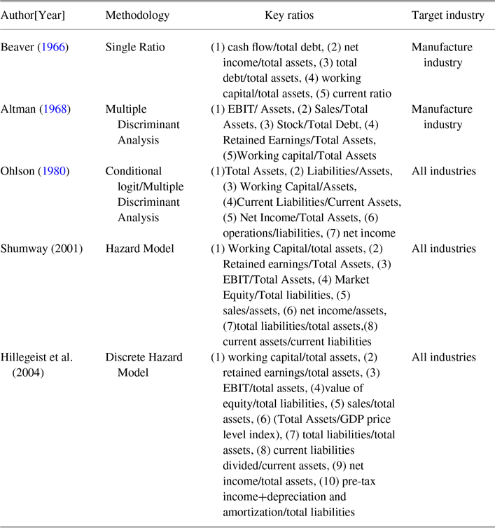
The results presented in Montebruno et al. (Reference Piero, Bennett, Harry and Carry2020) show that standard classification algorithms can be outperformed by machine learning algorithms. This confirms the value of extending the techniques traditionally used in this type of classification problem. Barboza et al. (Reference Flavio, Herbert and Edward2017) reviewed, re-evaluated and implemented other disciplines such as Altman’s Z-score, in conjunction with machine learning models. This comparison is something that other authors have also investigated, such as comparing the performance of the new models with the traditional models, as well as the one proposed by Altman. Since 1968, Altman’s Z-score has been considered a well-accepted model for predicting possible failures in companies Altman (Reference Altman1968). The main goal of Altman’s Z-score was to predict the bankruptcy of manufacturing companies, and later on its use was extended to other sectors. Hosaka (Reference Tadaaki2019) showed that convolutional neural networks performed better compared to methods using decision trees, linear discriminant analysis, support vector machines (SVMs), multilayer perceptron, AdaBoost or Altman’s Z-score. Wang et al. (Reference Nanxi2017) demonstrated that SVMs outperforms the back-propagation neural network in the problem of corporate bankruptcy prediction. This research has focused on comparing the model with the most frequently cited models and the most popular applications of traditional bankruptcy prediction. As shown in table 1, the authors have not considered the theory that has been developed in the period 1980 to 2001, due to the market crisis caused by turbulent historical events. Those events were Black Monday 1987 (Onnela et al. Reference Onnela, Anirban, Kimmo and Janos2003) and the Asian crisis 1997 (Wade and Veneroso Reference Robert and Frank1998), which had global repercussions on the economy. As shown in table 1, Altman and Beaver used information from the balance sheet and from the income statement. Altman’s model was initially created for bankruptcy prediction in manufacturing companies, although its application has since then been extended to all industries. However, the selected ratios are very similar for all companies, as they are the most indicative of any company’s financial health.
Previous research on bankruptcy prediction under the following headings: Author, Methodology, Attributes and ratios used, the Industry for which where developed.

The remainder of this study is organized as follows. The research objectives are presented in Section 2. The data and methodology design is described in Section 3. In Section 4, the implementation of the proposed method is outlined. In Section 5, the results and their implications are summarized. Finally, the conclusions drawn from the conducted research are discussed in Section 6.
2. Research Objectives
Regarding the gaps identified in the state-of-the-art, there is no method that can provide a comprehensive solution to all of them. For the purposes of this study, a bankruptcy binary classification problem has been considered with real-world data. Using traditional statistical methods and machine learning techniques, the aim of this research is to propose a methodology for the following three research objectives:
-
RO1: The possibility of predicting bankruptcy without considering numerous financial attributes, and without biasing the data for future machine learning classification algorithms. In the era of data and the contributions of big data to business (Saggi and Jain Reference Mandeep Kaur and Sushma2018), finding methodologies to reduce the amount of data needed to run algorithms is something that can greatly benefit companies.
-
RO2: How classification algorithms enable to predict bankruptcy according to the industry to which a company belongs, considering equal attributes. To evaluate how binary classification methods perform in each industry and to assess the relevance of the weight of each attribute according to a label in similar conditions (in this case financial attributes).
-
RO3: To avoid confusion by providing a decisive comparison of the performance of evaluation metrics in binary classification.
3. Data and Methods
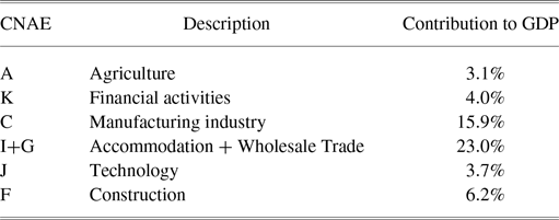
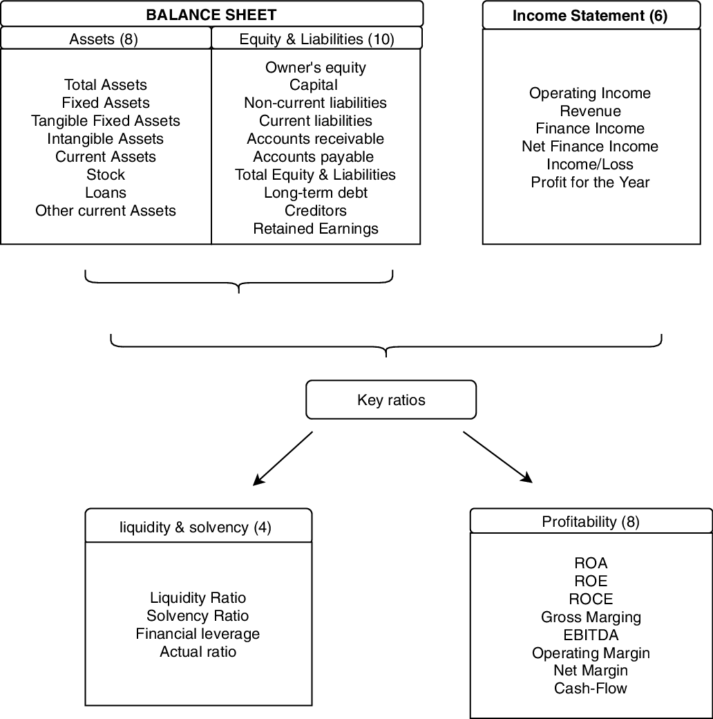
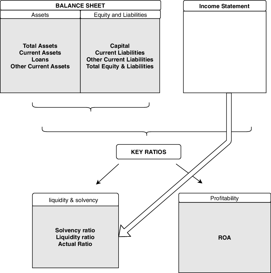
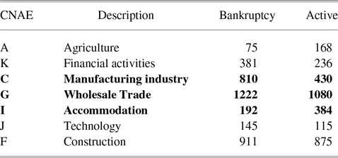
This study sampled companies across various industries from the “Sistema de Análisis de Balances Ibéricos” which belongs to the Orbis databaseFootnote 1. Only the firms that had relevant information available for the period (2016–2018 inclusive) have been included in our sample. The study has been carried out with real companies that belong to different industries. De Jong et al. (Reference Abe De, Rezaul and Thuy2008) have shown that the capital structure of a company is influenced not only by industry and company factors but also by country-specific factors. Li and Islam (Reference Larry and Silvia2019) demonstrated that industry-specific factors can both, directly and indirectly, affect a firm’s capital structure. One of the research objectives is to check the prediction ability of each algorithm, seeing how each algorithm is able to predict given the same variables, being different companies in different industries. Since the database and the study have been developed with information on the spanish companies, the industries that have been defined are industries that are the key contributors to the GDP in Spain. The industries and contribution % to GDP in 2018 (OECD 2018) are described in table 2. The CNAE code stands for the “Clasificación Nacional de Actividades Económicas,” or National Classification of Economic Activities, and is devised by the Spanish Statistical Institute. All the considered attributes are represented in Figure 1. The different ratios shown in Figure 1 have been used given the particularities of each industry in terms of the companies’ own financial structure. To be clearer, with respect to liquidity, a company in the retail industry will tend to have higher levels of liquidity than a company in the construction or restaurant industry. Companies in the retail sector are companies that pay their suppliers in installments as soon as the product is sold, and companies already invoice before they pay. In the construction sector, on the other hand, it is necessary to do some construction before paying. Therefore, one of the main goals of this methodology is to overcome the differences in the variety of data features, in this case in terms of financial structure when forecasting the bankruptcy of companies.
CNAE codes of industries considered in this work, as well as their contributions to the Spanish GDP

Initial Data

The choice covers the whole spectrum, from healthy to borderline firms, to avoid any selection bias. The classification criteria according to which companies have been identified are: the companies that were active in December 2018, as well as the companies that were in liquidation, bankruptcy or dissolution, and that had been categorized as bankrupt. A pre-processing procedure was applied to the data, including the removal of non-available values and outliers. The information for the two years prior to the study of the possibility of entering bankruptcy has been collected since it is the historical financial data that is required in the case of the Z-score (Altman Reference Altman1968). The dataset has been arbitrarily divided into two subsets; 80% of the data is used for a training set and 20% for the validation set. The dataset contains information on 3,600 companies that had gone bankrupt and 3,288 that are active. From among the companies in the dataset, some were missing important information and values. In those cases the company was not considered in the study. One-hot encoding has been done for the classification features. This process is advantageous because there is no ordinal relationship in the attribute. Active companies have been assigned a 1 (being the True class) and companies in bankruptcy a 0 (which is the false class).
3.1. Proposed Methodology
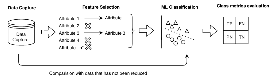
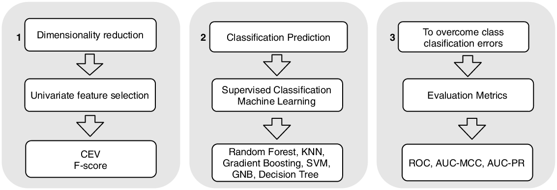
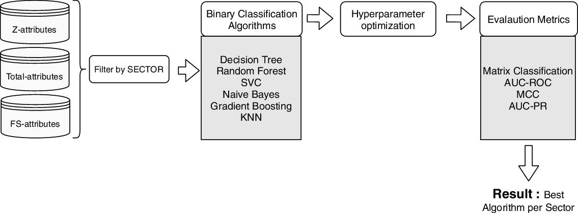
The overall methodology that has been developed that responds to the research objectives and is presented in Figures 2 and 3. Figure 2 describes the process in broad overview, while Figure 3 also outlines the methodologies used.
Proposed Method

Method Description. The columns are ordered and include an initial description of how the objectives are going to be achieved and the employed methodologies are presented in different subsections of this case study.

The attribute selection consists of reducing the number of attributes by analyzing the cumulative explained variance (CEV) and the F-score. The CEV is an analysis often used to analyze the data before doing a principal component analysis, nevertheless, in this case, it has also been used to reinforce feature extraction. Then, six supervised machine learning classification algorithms are compared to predict the probability of bankruptcy in the different samples of data. Finally, the algorithms’ class classification is evaluated, using the following evaluation metrics; Matthew correlation coefficient (MCC), area under curve – receiver operating characteristic (ROC-AUC) and area under curve – precision-recall (AUC-PR). A more detailed description concerning the different elements of the method is provided below. Univariate Feature Selection is described in 3.1.1, supervised machine learning classification algorithms in Section 3.1.2 and finally, Evaluation Metrics in Section 3.1.3.
3.1.1 Univariate feature selection
There are many well-known feature selection techniques for extracting the most representative attributes. Researches such as Solorio-Fernández et al. (Reference Saúl Solorio, J Ariel Carrasco and José Fco Martnez2020) and Chandrashekar and Sahin (Reference Girish and Ferat2014) analyzed the advantages and disadvantages of each feature selection concluding on the importance of each method depending on the input data. Also, Wen et al. (Reference Guoqiu, Xianxian, Yonghua, Linjun, Qimin and Malong2021) presented a dimensionality reduction approach for imbalanced datasets. In the case of the present research, feature selection is performed prior to the application of machine learning. Therefore, none of the feature selection methods that incorporate supervised learning or embedded techniques have been considered because they could bias the algorithms’ results, as Khaire and Dhanalakshmi (Reference Dhanalakshmi2019) demonstrated. For feature selection from the initial dataset, an F-score has been chosen because it can address the non-negative continuous nature of the variable, discarding alternatives like the chi-square metrics Kutlug Sahin et al. (Reference Emrehan Kutlug, Cengizhan and Taskin2017).
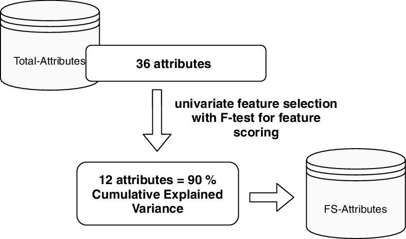
Figure 4 describes the process that starts at Total-attributes and finishes at FS-attributes. The univariate analysis has been the best option since the aim of this study is to identify the indicators that performed better individually and not to consider the interrelation between features Yang and Mao (Reference Feng and KZ2010). Univariate feature selection has been performed with F-test for feature scoring to this has made it possible to identify the most important ratios when determining a class.
Feature selection process. From Total-attributes through feature selection to FS-attributes

3.1.2. Supervised machine learning classification algorithms
Figure 5 summarizes the process that follows univariate selection. Considering the type of data and the fact that the problem to be solved involves predicting a binary label (the event of going bankrupt), supervised machine learning classification algorithms have been used. There are numerous supervised classification algorithms that have good results in different fields, as mentioned in Section 1. Those that have been widely used in bankruptcy prediction by different authors are compared in the study done by Olson et al. (Reference Olson, Dursun and Yanyan2012) and Barboza et al. (Reference Flavio, Herbert and Edward2017). The final list of the algorithms that have been considered in this study are: gradient boosting (GB) which builds the model in a stepwise and generalizes the model by allowing arbitrary optimization of a differentiable loss function Zięba et al. (2016), Gaussian Naive Bayes (NB) which is based on the Bayes theorem Eirola et al. (Reference Emil, Andrey, Anton, Kaj-Mikael, Yoan, DuŠan, Rui, Bo and Amaury2015) Sharma and Mavani (Reference Sharma and Monali2011), decision tree classifier which is based on a decision tree, is a predictive model that maps observations about an item to conclusions about the target value of the item Foroghi et al. (Reference Daryush and Amirhassan2011), random forest (RF) which consists on a combination of predictor trees such that each tree depends on the values of a random vector tested independently and with the same distribution for each predictor tree, K-nearest neighbors (KNNs) which seeks out the closest observations that are trying to be predicted and classifies the point of interest based on the most data surrounding it, Imandoust and Bolandraftar (Reference Sadegh Bafandeh and Mohammad2013) and support vector machine classifier (SVMC) which is based on the hyperplane concept Hsu et al. (Reference Chih-Wei, Chih-Chung and Chih-Jen2003). To overcome the potential bias when training the algorithms, fivefold cross-validation was used.The cross-validation technique has made it possible to reduce the problems of overfitting and also evaluate the results of the analysis while ensuring that they are independent of the partitioning between training and test data. As shown in Figure 5, a Grid Search for hyperparameter tuning has also been applied in order to improve the algorithm’s classification results. The Grid Search technique has been implemented to find the optimal hyperparameters for each of the models, which results in a model with greater prediction accuracy.
Method and research process presented in the proposed case study.

3.1.3. Evaluation Metrics
The three metrics that have been considered are; ROC-AUC, MCC, and AUC-PR. When applying a classification algorithm to a dataset for class prediction, one of the most crucial factors to be evaluated is algorithm performance. There are different options for determining the accuracy of the algorithm. For example, any well-known metric could be used, however, it would only be able to indicate the overall performance, but it would not be able to identify false positives or false negatives. This occurs when an algorithm identifies one class as another, incurring statistical error types I and II, which leads to False Negatives and False Positives. The ROC is an approach to evaluating the precision of the algorithms. ROC gives a graphical representation of the sensitivity to specificity for a binary classification system as the discrimination threshold is varied. For instance, when X is the continuous random variable which is predicted to make the classification, i.e., the assigned class will be the “positive” one if
 $X\geq\theta$
for a certain threshold
 $\theta$
and the negative one otherwise. Let
 $f_+$
be the probability density of t when the actual class is the “positive” one, and
 $f_-$
otherwise. Thus, the true positive rate is given as a function of the threshold
 \begin{equation} \text{TPR}(\theta)=\int_\theta^\infty f_+(X) \mathrm{d} t\,.\end{equation}
Similarly, the false positive rate is given by
 \begin{equation} \text{FPR}(\theta)=\int_\theta^\infty f_-(X) \mathrm{d} t\,.\end{equation}
The ROC curve is the parametric plot defined by the points
 $\left\{{\text{TPR}(\theta),\text{FNR}(\theta)}\right\}$
, and hence its area is given by
 \begin{equation} \text{AUC}=\int_\infty^{-\infty} \text{TPR}'(\theta)\text{FPR}(\theta) \mathrm{d} t\,,\end{equation}
which can be numerically approximated using the predictions for the test set. To visualize the performance, the AUC of the ROC has been incorporated in the results as well as the MCC. Regarding the variety of data, in the case of the results obtained when separating the data per industry, some of the industry data batches were class imbalanced. In the area of bankruptcy prediction, it has been studied that the characteristics of an imbalanced dataset bias the performance of the algorithm Veganzones and Séverin (Reference David and Eric2018). Therefore, evaluation metrics must be employed He and Garcia (Reference Haibo and Edwardo2009), Davis and Goadrich (Reference Jesse and Mark2006). For example, the ones referenced above, perform better than ROC in this situation because they do not take into consideration the classes that cause the dataset to be imbalanced. To contrast the ROC-AUC and the MCC Chicco and Jurman (Reference Davide and Giuseppe2020), the AUC of the PR has been considered as an alternative Saito and Rehmsmeier (Reference Takaya and Marc2015). The PR curve is similar to the ROC curve, following parametrization
 $\left\{{\text{R}(\theta),\text{P}(\theta)}\right\}$
where
 \begin{equation} \text{P}(\theta)=\frac{\text{TPR}(\theta)}{\text{TPR}(\theta)+\text{FPR}(\theta)}\,\end{equation}
is the precision and
 \begin{equation} \text{R}(\theta)=\text{TPR}(\theta)\,\end{equation}
is the recall, which is equivalent to the TPR as noted.
4. Methodology Implementation
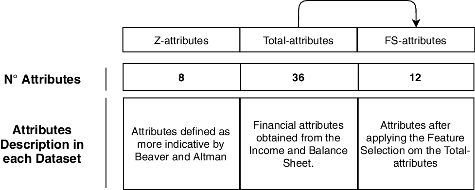
Figure 6 describes the three research objectives that have been analyzed and used in the machine learning classification process.
Dataset description

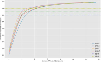
The among the attributes described in table 1, those that Altman and Beaver considered most indicative of bankruptcy have been identified as Z-attributes, considering the 8 that were different, secondly the 36 most signified features of the Balance Sheet and Income Statement and the liquidity ratios have been identified as Total-attributes. Finally, the attributes resulting from the univariate feature2 selection with F-test for feature scoring have been identified as FS-attributes. Once all the data had been identified, the feature selection process was applied. The first step has been to identify the point at which all the CEV was at more than 90% in all industries, so we could identify the number of principal components required as in Figure 7 and then to identify the attributes by applying univariate F-score.
Cumulative explained variance

Regarding dimensionality reduction, the results led to the selection of the 12 attributes that are described in Figure 8. The ratios have been added to see how the calculation, or choosing some ratios over others, affects the industry and therefore the nature of the financial structure of each of the companies. As Beaver et al. (Reference Beaver, McNichols and Jung-Wu2005) analyzed, the ratios are attributes that provide a lot of information about bankruptcy prediction. This is evidenced in the results obtained after feature selection. Once the three data batches had been processed as shown in Figure 6, all of them have been analyzed. Machine learning classification algorithms have been applied to each of the sets and in turn to each of the industries. To maximize the performance of the algorithms, hyperparameter tuning has been applied so that each of the algorithms is better adjusted to each of the datasets and industries. The results of the classification predictions have been evaluated with the MCC-AUC, PR-AUC, and the ROC-AUC.
Final Data

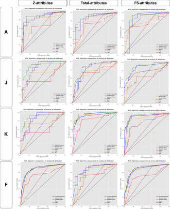
ROC-AUC algorithms per industry. In this Figure, the industries A, J, K, and F are compared

5. Results and discussion
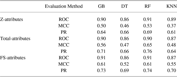
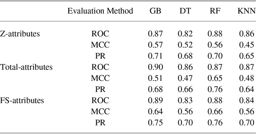
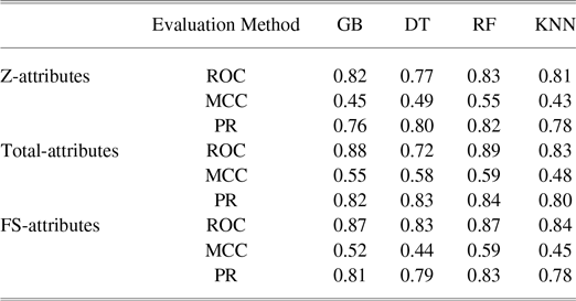
This section presents the results obtained after applying the proposed methodology. In order to obtain the results of the comparison of the different evaluation algorithms and metrics, the same classification algorithms and evaluation metrics have been applied indistinctly to all industries in the three sub-data batches (Z-attributes, Total-attributes, and FS-attributes). As shown in table 3, GB and RF have had very similar performance and good class classification in all cases, which has also been reported in the research of Montebruno et al. (Reference Piero, Bennett, Harry and Carry2020). However, in this case we have not only evaluated the results with the ROC-AUC and the confusion matrix, we have also added two more evaluation metrics. In the results provided by our research, the ROC-AUC evaluation metric always achieves the highest results. In fact, when all datasets are merged and evaluated together, all evaluation metrics achieve high results, and ROC-AUC is always above 0.90. As can be seen in the results, there is a big difference between the scores provided by ROC-AUC and those of AUC-MCC. In Table 3 it can be seen that the AUC-MCC results hardly reach more than 0.65.
Evaluation metrics for all industries

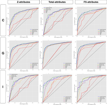
When the comparison has been done per industry the evaluation metrics also show that the GB and RF are the algorithms outperform the others, as shown in Figure 10 whereas SVMC and KNN have had the worst results. These results are different from the Wang et al. (Reference Nanxi2017) research but coincide with the research of Devi and Radhika (Reference Sarojini Devi and Radhika2018) which identified that it was difficult for SVMCs to perform well in bankruptcy prediction when the volume of data increased, even though their performance can be the best if trained jointly with a hybrid switching particle swarm optimization. Logically, both GB and RF perform well as both are ensemble methods and the structure of the operation is very similar. Considering the mathematics behind each algorithm, GB builds trees one at a time, which means that a new tree can help correct previous errors. RF trains each tree independently, using a random sample of the data. In relation to whether the outcome differs in the sectors due to the importance of the financial structure and the industry, as considered in Li and Islam (Reference Larry and Silvia2019), in our research it has not been possible to draw conclusive results.
ROC-AUC algorithms per industry. In this Figure, the industries C, G, and I are compared

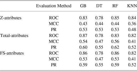
The distribution of the class classifications is described in table 4. To asses the impact of the distribution of the class in a given dataset when using a classification algorithm, the extended detail has been collected in three tables. The Industries: C (Manufacturing), G (Wholesale Trade) and I (Accommodation) have been selected for further analysis because in terms of label balance, C and G are the most imbalanced ones and I is the most balanced one and the ones containing more volume of data.
-
Table 5 shows that in industry G, in the Total-attributes and FS-attributes, the GB is the best option when it is evaluated with the ROC-AUC metrics, but when considering the other evaluation metrics (PR-RC and MCC), RF performs better.
-
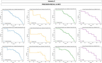
Table 6 has more companies labeled as bankrupt and contains information on Industry C and GB outperforms on ROC-AUC metrics.
-
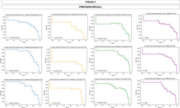
Table 7 shows that if only the ROC-AUC results had been considered as an evaluation metric for industry I, RF would have had the best performance, followed by GB.
GDP and company industry distribution. The rows market in bold type, are the ones that will be analyzed further since the datasets are imbalanced in type of label

As can be derived from the results when considering the batch of Total-attributes, the results lead to the conclusion that GB performs better when considering ROC-AUC metrics. Nonetheless, the other evaluation metrics indicate that RF performs better. The plots to visualize the performance of the evaluation metric of the AUC-PR are shown in Figure 12.
Evaluation metrics for Companies Industry G

Evaluation metrics for Companies Industry C

Evaluation metrics for Companies Industry I

Industry C

Industry I

In the tables above, the results given for balanced and imbalanced data demonstrate that the choice of an evaluation metric depends on the balance/imbalance of the input data in terms of class. Another interesting result derived from the evaluation metrics is that the algorithm classifies better in terms of class when dimensionality reduction has been previously applied. As for the data and ratios applied in the literature by other authors (Z-attributes), the results show that the attributes, after the application of dimensionality reduction (FS-attributes), allow for similar results in terms of the scoring of evaluation metrics. classification algorithms.
6. Conclusions
The aim of this research has been to develop a methodology for predicting in binary class problems. The objective has been to develop a methodology so that when comparing the prediction performance of classification algorithms, the evaluation metrics used can be decisive or can infer erroneous decisions in terms of goodness of fit. The results lead to the conclusion that when applying machine learning classification algorithms, the feature reduction generated by the univariate model performs as good as the traditional attributes chosen by specialists in the field, such as the attributes selected by Altman in the Z-score model. Furthermore, in an attempt to identify an algorithm that could perform better in the analysis of companies in a certain industry, the results are not conclusive. One of the most important results obtained in the research is that the evaluation metrics are decisive when choosing an algorithm for predicting the classifications. In this paper, it has been demonstrated that when evaluating the different algorithms all the possible metrics have to be considered to avoid biased conclusions. Using only one evaluation metric can lead to errors in further applications. This paper compared and concluded the progress of classification machine learning models and the importance of the evaluation metrics with respect to bankruptcy prediction.
Acknowledgments
This research has been supported by the project “INTELFIN: Artificial Intelligence for investment and value creation in SMEs through competitive analysis and business environment,” Reference: RTC-2017-6536-7, funded by the Ministry of Science, Innovation and Universities (Challenges-Collaboration 2017), the State Agency for Research (AEI) and the European Regional Development Fund (ERDF).
Declarations of Competing Interest
None.
CRediT authorship contribution statement
María E. Pérez-Pons: Data curation, Formal analysis, Investigation, Writing - original draft, Writing - review and editing. Javier Parra-Dominguez: Conceptualization, Investigation, Methodology, and Writing - review and editing. Guillermo Hernández: Data curation, Formal analysis, Methodology, Writing - review and editing, and Software Supervision. Enrique Herrera-Viedma: Writing - review and editing and Supervision. Juan M.Corchado: Conceptualization, writing - review and editing and Supervision.