1. Introduction
As offshore wind farms become larger, their interaction with the atmosphere becomes important to their operation (Bleeg et al. Reference Bleeg, Purcell, Ruisi and Traiger2018; Porté-Agel, Bastankhah & Shamsoddin Reference Porté-Agel, Bastankhah and Shamsoddin2020; Fischereit et al. Reference Fischereit, Brown, Larsén, Badger and Hawkes2021). Recent large-eddy simulation (LES) studies have identified wind-farm-induced gravity waves as contributing to the so-called blockage phenomenon, where the wind is slowed down upstream of the farm, thereby reducing turbine power output (Allaerts & Meyers Reference Allaerts and Meyers2017, Reference Allaerts and Meyers2018; Lanzilao & Meyers Reference Lanzilao and Meyers2022, Reference Lanzilao and Meyers2023b, Reference Lanzilao and Meyers2024; Maas Reference Maas2022, Reference Maas2023; Stipa et al. Reference Stipa, Ajay, Allaerts and Brinkerhoff2024a).
Offshore, the atmosphere frequently has a structure similar to a conventionally neutral boundary layer (CNBL), where a neutral atmospheric boundary layer (ABL) is topped by a capping inversion and a stably stratified free atmosphere (Csanady Reference Csanady1974; Smedman, Bergström & Grisogono Reference Smedman, Bergström and Grisogono1997). Gravity waves can appear in these conditions, with waves generated by surface topography being extensively studied (Klemp & Lilly Reference Klemp and Lilly1975; Durran Reference Durran1990; Vosper Reference Vosper2004; Smith Reference Smith2007; Teixeira Reference Teixeira2014; Sachsperger, Serafin & Grubišić Reference Sachsperger, Serafin and Grubišić2015). As first hypothesized by Smith (Reference Smith2010), wind farms can also trigger such gravity waves. By slowing down the ABL flow, they push the capping inversion upwards, thereby initiating gravity waves both within the inversion layer and in the free atmosphere aloft. The pressure perturbations of these waves in turn affect the flow in the ABL, leading to blockage upstream of the farm, and pressure gradients throughout it (Allaerts & Meyers Reference Allaerts and Meyers2017).
While LES studies are a useful tool to gain insight into the flow physics, their high cost prevents them from being used for wind farm planning and control (Meyers et al. Reference Meyers, Bottasso, Dykes, Fleming, Gebraad, Giebel, Göçmen and van Wingerden2022). Conventional wake models, which focus on the downstream effects of individual turbines (e.g. Bastankhah & Porté-Agel Reference Bastankhah and Porté-Agel2014), cannot account for the complex mesoscale effects of large-scale interactions between wind farms and the ABL (Porté-Agel et al. Reference Porté-Agel, Bastankhah and Shamsoddin2020; Centurelli et al. Reference Centurelli, Vollmer, Schmidt, Dörenkämper, Schröder, Lukassen and Peinke2021). Over the years, several approaches have been developed to estimate the global atmospheric response of large wind farms. For instance, the upper limit of wind farm power production has been studied using so-called ‘top-down’ models, which estimate the available energy density for infinitely large wind farms (Frandsen Reference Frandsen1992; Frandsen et al. Reference Frandsen, Barthelmie, Pryor, Rathmann, Larsen, Højstrup and Thøgersen2006; Emeis Reference Emeis2009; Calaf, Meneveau & Meyers Reference Calaf, Meneveau and Meyers2010; Abkar & Porté-Agel Reference Abkar and Porté-Agel2013). This approach has also been extended to include entrance and turbine wake effects (Stevens, Gayme & Meneveau Reference Stevens, Gayme and Meneveau2015; Luzzatto-Fegiz & Caulfield Reference Luzzatto-Fegiz and Caulfield2018). However, these models focus on turbulent entrainment, and do not include blockage or atmospheric gravity waves.
Mesoscale climate and weather models can fully capture the atmospheric response to wind farms, and have included various wind farm parametrizations (Fischereit et al. Reference Fischereit, Brown, Larsén, Badger and Hawkes2021). However, the computational cost of these models is high and their resolution relatively coarse. They do not model turbine–turbine interactions explicitly, as these occur on smaller scales. Recent research by Nishino & Dunstan (Reference Nishino and Dunstan2020) produced an elementary way of coupling these large-scale flow models to turbine-level simulations, by ensuring that the two scales predict the same mean velocity over the farm. While this has produced good agreement with LES for infinite wind farms (Kirby, Nishino & Dunstan Reference Kirby, Nishino and Dunstan2022), it still requires expensive numerical models to estimate the atmospheric response for a given farm (Patel, Dunstan & Nishino Reference Patel, Dunstan and Nishino2021). Very recently, Kirby, Dunstan & Nishino (Reference Kirby, Dunstan and Nishino2023) developed an analytical approach of estimating the momentum availability for a given farm, but does not yet include the effect of upper atmosphere stratification.
Inexpensive linear models of atmospheric gravity waves have been used in mountain wave research for decades (Teixeira Reference Teixeira2014). As first proposed by Smith (Reference Smith2010), these models could predict the effects of wind-farm-induced gravity waves as well. Allaerts & Meyers (Reference Allaerts and Meyers2019) built on Smith's idea, and produced an atmospheric perturbation model (APM), so named because the effect of the wind farm is modelled as a linear perturbation on the atmospheric flow. It divides the vertical structure of the ABL into two layers of vertically averaged flow, topped by a capping inversion and the stratified free atmosphere. The flow in the ABL layers is modelled explicitly, while the gravity waves are incorporated as a closure equation for the pressure perturbation (Smith Reference Smith2010; Devesse et al. Reference Devesse, Lanzilao, Jamaer, Van Lipzig and Meyers2022). In past studies, the model has been called the three-layer model (TLM/3LM), but as more layers can be added (Devesse et al. Reference Devesse, Lanzilao, Jamaer, Van Lipzig and Meyers2022), we will call it the APM. As a simplified mesoscale model, it is relatively fast, and has shown potential for both wind farm control (Lanzilao & Meyers Reference Lanzilao and Meyers2021b) and annual energy production estimates (Allaerts et al. Reference Allaerts, Vanden Broucke, Van Lipzig and Meyers2018).
The goal of this paper is to improve the representation of wind farms in the APM. As a highly simplified model, the APM cannot resolve turbine-level flows, due to its height-averaged modelling approach and coarse grid resolution. Additionally, it does not explicitly model turbulence. Therefore, when simulating large wind farms, the turbine forces, the increase in turbulent momentum entrainment and the dispersive stresses from the subgrid flow heterogeneity have to be parametrized. Previous studies with the APM neglected the latter two, and represented the wind farm purely in terms of turbine forcing (Allaerts & Meyers Reference Allaerts and Meyers2019; Devesse et al. Reference Devesse, Lanzilao, Jamaer, Van Lipzig and Meyers2022; Stipa, Allaerts & Brinkerhoff Reference Stipa, Allaerts and Brinkerhoff2024b). However, based on the LES results from Lanzilao & Meyers (Reference Lanzilao and Meyers2024), we find that the increased turbulent momentum flux and dispersive stresses are important to the mesoscale flow. Therefore, we develop parametrizations to represent them in the APM.
Dispersive stresses have been found to be important in sparse canopy flows, which include large wind farms (Markfort, Zhang & Porté-Agel Reference Markfort, Zhang and Porté-Agel2012; Brunet Reference Brunet2020). In such flows, they primarily play a role at the canopy entrance, as large unresolved flow features develop (Moltchanov, Bohbot-Raviv & Shavit Reference Moltchanov, Bohbot-Raviv and Shavit2011). Typically, these stresses are difficult to parametrize, as the smaller-scale flows are not modelled and highly dependent on the underlying canopy structure. In contrast, the turbine-scale flows in wind farms consist primarily of the turbine wakes, which are relatively well-structured and can be approximated using simple engineering models (Porté-Agel et al. Reference Porté-Agel, Bastankhah and Shamsoddin2020). We leverage this in the development of a basic parametrization.
This requires the APM to couple to a wake model. Allaerts & Meyers (Reference Allaerts and Meyers2019) took the background velocity, to which the wake model adds the turbine wakes, to be constant and equal to the velocity at some distance upstream of the farm entrance (i.e. 10 times the turbine diameter). This approach, while effective at providing a rough estimate of the blockage effect, is very ad hoc, and cannot take into account the influence of mesoscale phenomena downstream of the farm entrance. This is an important shortcoming, as for instance the favourable pressure gradients associated with gravity waves can increase the power output of downstream turbines (Allaerts & Meyers Reference Allaerts and Meyers2017; Lanzilao & Meyers Reference Lanzilao and Meyers2022, Reference Lanzilao and Meyers2023b, Reference Lanzilao and Meyers2024; Maas Reference Maas2022, Reference Maas2023). Very recently, Stipa et al. (Reference Stipa, Allaerts and Brinkerhoff2024b) improved on this by calculating a background velocity for the wake model based on the APM pressure estimates. We take a different approach, and present a new wake model coupling method based on matching the velocity between the wake model and the APM. In addition, both the new wake model coupling and APM are validated using 27 simulations of a finite wind farm with varying levels of stratification from the LES dataset developed by Lanzilao & Meyers (Reference Lanzilao and Meyers2024).
The new coupling method sets up a background velocity for the wake model that ensures a velocity field that is consistent with the APM output. This results in good agreement for both the velocity fields and the turbine power production, provided that the wake model gives a realistic estimation of the turbine-level flow throughout the farm. When analysing the LES cases from Lanzilao & Meyers (Reference Lanzilao and Meyers2024), we find that this requires the inclusion of a turbine induction model. To this end, we use the model proposed by Troldborg & Meyer Forsting (Reference Troldborg and Meyer Forsting2017). We use the wake-merging method of Lanzilao & Meyers (Reference Lanzilao and Meyers2021a), as it allows for varying background velocities throughout the farm.
The remainder of this paper is structured as follows. Section 2 re-derives and describes the APM, and performs a momentum budget analysis to identify the most important physical effects. Section 3 discusses the wake model used in this work, and develops the new coupling method. Section 4 performs an a priori validation of the coupling method using the LES dataset developed by Lanzilao & Meyers (Reference Lanzilao and Meyers2024), and an a posteriori validation of the complete APM against the same data. Finally, § 5 gives some conclusions and suggestions for further research.
2. Atmospheric perturbation model
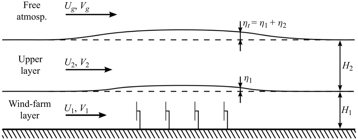
To model the interaction between wind farms and atmospheric gravity waves, this paper further develops the APM introduced by Allaerts & Meyers (Reference Allaerts and Meyers2019). It is a reduced-order model, where the ABL is treated as two vertically uniform layers of fluid. In the lower layer, also called the wind farm layer, the effect of the turbine forces is felt directly, while the upper layer consists of the remainder of the ABL. These layers are divided by pliant surfaces, so that there is no mass flux between them. The capping inversion, which separates the upper layer and the free atmosphere, also limits momentum flux (Taylor & Sarkar Reference Taylor and Sarkar2008). Figure 1 conceptually shows the resulting model structure. The model consists of two continuity and momentum equations, one for each layer, and a closure equation that links the thickening of the ABL to the pressure feedback of the gravity waves in the free atmosphere. This section provides an overview of the model's derivation, and its parametrization of gravity waves, turbulent momentum fluxes and wind farm effects.
Schematic representation of the atmospheric perturbation model. Figure from Allaerts & Meyers (Reference Allaerts and Meyers2019), reproduced with permission.

In their original derivation of the APM, Allaerts & Meyers (Reference Allaerts and Meyers2019) added the wind farm forces to the model after the governing equations were derived. This implicitly introduced a filtering operation, in order to represent the relatively small-scale turbines in the mesoscale model. We largely follow Allaerts & Meyers (Reference Allaerts and Meyers2019), but explicitly apply this filtering operation and turbine forcing throughout the derivation, which will result in additional dispersive stresses.
2.1. Derivation
In the derivation of the APM, two operations are applied to the momentum and continuity equations: a horizontal filtering to obtain the mesoscale flow and a height-averaging to reduce the order of the model (Allaerts & Meyers Reference Allaerts and Meyers2019). The former is done through a Gaussian filter, defined as
 \begin{equation} \bar{\phi}(x,y) = \iint_{L_x \times L_y}{G_\ell(x-x^{\prime},y-y^{\prime}) \phi(x^{\prime},y^{\prime})}\,\mathrm{d}\kern0.06em x^{\prime}\,\mathrm{d}y^{\prime},\quad \phi = \bar{\phi} + \phi^{\prime\prime}, \end{equation}
where  $L_x \times L_y$ is the APM domain size and
 $G_\ell$ is a Gaussian kernel with length
 $\ell$ (Allaerts & Meyers Reference Allaerts and Meyers2019):
 \begin{equation} G_\ell(x,y)=\frac{1}{{\rm \pi} \ell^2}\exp{\left(-\frac{x^2+y^2}{\ell^2}\right)}. \end{equation}
Since the APM reduces the vertical structure of the ABL to two averaged layers, we try to have a horizontal resolution similar to the ABL height. Therefore, we follow Allaerts & Meyers (Reference Allaerts and Meyers2019) in taking  $\ell =1\ \mathrm {km}$, which should suffice for typical offshore boundary layers.
The flow is then split into three layers, bounded by the ground and the pliant surfaces  $z_1$ and
 $z_2$, as sketched in figure 1. The lower surface
 $z_1$ divides the ABL into a lower layer, where the turbine forces are felt directly, and an upper layer, which comprises the remainder of the ABL. The third layer of the APM consists of the free atmosphere above the ABL. The surfaces
 $z_1$ and
 $z_2$ are defined as
 $$\begin{gather} \bar{w}(x,y,z_1)=\bar{\boldsymbol{u}}_h(x,y,z_1)\boldsymbol{\cdot}\boldsymbol{\nabla}_h z_1, \end{gather}$$
 $$\begin{gather}\bar{w}(x,y,z_2)=\bar{\boldsymbol{u}}_h(x,y,z_2)\boldsymbol{\cdot}\boldsymbol{\nabla}_h z_2, \end{gather}$$
where  $w$ is the vertical velocity and
 $\boldsymbol {u}_h$ and
 $\boldsymbol {\nabla }_h$ are the two-dimensional horizontal velocity vector and del operator, respectively. Far upstream of the farm, we set
 $z_1$ and
 $z_2$ at twice the hub height and the capping inversion height respectively (Allaerts & Meyers Reference Allaerts and Meyers2019). Note that
 $z_1$ and
 $z_2$ are not the filtered pliant surfaces, but rather the pliant surfaces in the filtered flow, as this greatly simplifies the derivation below. However, this difference is negligible in practice.
We now define the height-averaging operator:
 $$\begin{gather} \langle\bar{\phi}\rangle_1=\frac{1}{z_1}\int_{0}^{z_1}\bar{\phi}(z)\,\mathrm{d}z, \end{gather}$$
 $$\begin{gather}\langle\bar{\phi}\rangle_2=\frac{1}{z_2-z_1}\int_{z_1}^{z_2}\bar{\phi}(z)\,\mathrm{d}z, \end{gather}$$
where the subscripts 1 and 2 correspond to the lower and upper layer, respectively. Fluctuations around the height-averaged state are denoted using triple primes, so that  $\bar {\phi } = \langle \bar {\phi }\rangle _i + \bar {\phi }_i^{\prime \prime \prime }$ in layer
 $i$. We denote the resulting layer thicknesses with
 $h_1$ and
 $h_2$.
To obtain the APM governing equations, these operators are applied to the steady-state, Reynolds-averaged, incompressible continuity and momentum equations. In doing so, the vertical velocity and the associated momentum equation drop out, analogous to the derivation of the shallow-flow equations (Allaerts & Meyers Reference Allaerts and Meyers2019). Appendix A shows this procedure in detail for the lower-layer continuity equation. The end result is a continuity and momentum equation for each of the two layers:
 $$\begin{gather} \boldsymbol{\nabla}_h\boldsymbol{\cdot}(h_1\langle\bar{\boldsymbol{u}}_h\rangle_{1})=0, \end{gather}$$
 $$\begin{gather}\boldsymbol{\nabla}_h\boldsymbol{\cdot}(h_2\langle\bar{\boldsymbol{u}}_h\rangle_{2})=0, \end{gather}$$
 \begin{align} \langle\bar{\boldsymbol{u}}_h\rangle_{1}\boldsymbol{\cdot}\boldsymbol{\nabla}_h \langle\bar{\boldsymbol{u}}_h\rangle_{1} &=-\frac{1}{\rho_0}\boldsymbol{\nabla}_h\langle\,\bar{p}\rangle_1 - f_c\boldsymbol{\mathsf{J}}\boldsymbol{\cdot}(\boldsymbol{U}_{g,h} - \langle\bar{\boldsymbol{u}}_h\rangle_{1}) + \boldsymbol{\nabla}_h\boldsymbol{\cdot}\langle\bar{\boldsymbol{\tau}}_{hh}\rangle_1 + \frac{\bar{\boldsymbol{\tau}}_{h3,1}-\bar{\boldsymbol{\tau}}_{h3,0}}{h_1} \nonumber\\ &\quad + \langle\,\bar{\boldsymbol{f}}_{{wf}}\rangle_1 - \langle\boldsymbol{\nabla}\boldsymbol{\cdot}(\boldsymbol{\tau}_{d,h})\rangle_1 - \frac{1}{h_1}\boldsymbol{\nabla}_h\boldsymbol{\cdot}(h_1\langle \bar{\boldsymbol{u}}_{h,1}^{\prime\prime\prime} \bar{\boldsymbol{u}}_{h,1}^{\prime\prime\prime}\rangle_1) + \frac{\boldsymbol{\mathcal{R}}_1}{h_1}, \end{align}
 \begin{align} \langle\bar{\boldsymbol{u}}_h\rangle_{2}\boldsymbol{\cdot}\boldsymbol{\nabla}_h \langle\bar{\boldsymbol{u}}_h\rangle_{2} &=-\frac{1}{\rho_0}\boldsymbol{\nabla}_h \langle\,\bar{p}\rangle_2 - f_c\boldsymbol{\mathsf{J}}\boldsymbol{\cdot}(\boldsymbol{U}_{g,h} - \langle\bar{\boldsymbol{u}}_h\rangle_{2}) + \boldsymbol{\nabla}_h\boldsymbol{\cdot}\langle\bar{\boldsymbol{\tau}}_{hh}\rangle_2 - \frac{\bar{\boldsymbol{\tau}}_{h3,1}}{h_2} \nonumber\\ &\quad -\langle\boldsymbol{\nabla}\boldsymbol{\cdot}(\boldsymbol{\tau}_{d,h})\rangle_2 - \frac{1}{h_2}\boldsymbol{\nabla}_h\boldsymbol{\cdot}(h_i\langle\bar{\boldsymbol{u}}_{h,2}^{\prime\prime\prime} \bar{\boldsymbol{u}}_{h,2}^{\prime\prime\prime}\rangle_2) + \frac{\boldsymbol{\mathcal{R}}_2}{h_2}, \end{align}
where the indices 1 and 2 indicate the layer number and the subscripts  $h$ and 3 indicate horizontal and vertical components, respectively. Furthermore,
 $\rho _0$ is the air density,
 $p$ is the pressure perturbation,
 $f_c$ is the Coriolis parameter,
 $\boldsymbol{\mathsf{J}}=\boldsymbol {e}_x\boldsymbol {e}_y-\boldsymbol {e}_y\boldsymbol {e}_x$ is the two-dimensional rotation dyadic (with
 $\boldsymbol {e}_x$ and
 $\boldsymbol {e}_y$ the unit vectors in the
 $x$ and
 $y$ directions, respectively),
 $\boldsymbol {U}_{g,h}$ is the horizontal geostrophic wind and
 $\bar {\boldsymbol {\tau }}_{hh}$ is the horizontal turbulent momentum flux. Large-scale pressure gradients are included through the geostrophic balance as
 $f_c\boldsymbol{\mathsf{J}}\boldsymbol{\cdot}\boldsymbol {U}_{g,h}$. Additionally,
 $\boldsymbol {\tau }_{h3,0}$ and
 $\boldsymbol {\tau }_{h3,1}$ are the vertical turbulent kinetic shear stresses at the ground and between the ABL layers, respectively. The wind farm force, also filtered in the horizontal plane, is denoted with
 $\bar {\boldsymbol {f}}_{{wf}}$. The two penultimate terms in (2.9) and (2.10) are the height-averaged dispersive stresses and the Taylor-shear dispersion, which appear as the filtering and height-averaging operators are applied to the convective acceleration. Allaerts & Meyers (Reference Allaerts and Meyers2019) did not include the former, as they did not explicitly apply the filtering operation. Because they are related to the unresolved flow, we denote them as subgrid terms throughout this paper. The dispersive stresses are given by
 \begin{equation} \boldsymbol{\tau}_{d,h} = \overline{\boldsymbol{u}\boldsymbol{u}_h}-\bar{\boldsymbol{u}} \bar{\boldsymbol{u}}_h. \end{equation}
Finally,  $\boldsymbol {\mathcal {R}}_1$ and
 $\boldsymbol {\mathcal {R}}_2$ are residual terms related to the vertical structure of the flow (Allaerts & Meyers Reference Allaerts and Meyers2019):
 \begin{align} \boldsymbol{\mathcal{R}}_1 &= \frac{1}{\rho_0}(\,\bar{p}\vert_{z_1}- \langle\,\bar{p}\rangle_1) \boldsymbol{\nabla}_h z_1 - (\bar{\boldsymbol{\tau}}_{hh}\vert_{z_1}- \langle\bar{\boldsymbol{\tau}}_{hh}\rangle_1) \boldsymbol{\cdot} \boldsymbol{\nabla}_h z_1, \end{align}
 \begin{align} \boldsymbol{\mathcal{R}}_2 &= \frac{1}{\rho_0}(\,\bar{p}\vert_{z_2}-\langle\,\bar{p}\rangle_2)\boldsymbol{\nabla}_h z_2 - \frac{1}{\rho_0}(\,\bar{p}\vert_{z_1}-\langle\,\bar{p}\rangle_2)\boldsymbol{\nabla}_h z_1 \nonumber\\ &\quad -(\bar{\boldsymbol{\tau}}_{hh}\vert_{z_2}-\langle\bar{\boldsymbol{\tau}}_{hh}\rangle_2) \boldsymbol{\cdot} \boldsymbol{\nabla}_h z_2 +(\bar{\boldsymbol{\tau}}_{hh}\vert_{z_1}- \langle\bar{\boldsymbol{\tau}}_{hh}\rangle_2)\boldsymbol{\cdot} \boldsymbol{\nabla}_h z_1. \end{align}
Equations (2.7)–(2.10) provide the governing equations for the APM, with the layer thicknesses and velocities  $(\langle \bar {\boldsymbol {u}}_h\rangle _{1},h_1)$ and
 $(\langle \bar {\boldsymbol {u}}_h\rangle _{2},h_2)$ as state variables. So far, these equations are exact, aside from the assumption that the capping inversion suppresses the vertical turbulent momentum fluxes at the top of the ABL. Following Allaerts & Meyers (Reference Allaerts and Meyers2019), we drop the residual terms based on an LES-based momentum budget analysis (see § 2.4).
2.2. Parametrizations
We now go through the remaining terms in the momentum equations, and provide closure equations and parametrizations.
2.2.1. Gravity waves
The displacement of the capping inversion  $\eta _t$, sketched in figure 1, causes gravity waves both within the inversion layer and in the free atmosphere above. These waves then induce a pressure perturbation
 $p_t$ at the top of the ABL, which is given by (Smith Reference Smith2010)
 \begin{equation} \frac{p_t}{\rho_0}=g^{\prime}\eta_t+\mathcal{F}^{-1}(\varPhi)*\eta_t, \end{equation}
where  $\eta _t=h_1+h_2-H$, with
 $H$ being the unperturbed ABL height,
 $\mathcal {F}^{-1}$ is the inverse Fourier transform and
 $*$ denotes a convolution. The ABL is assumed to be hydrostatic, so the pressure perturbation in both layers is equal to this
 $p_t$. The first term in the above equation gives the pressure feedback of the inversion waves, which directly scales with the reduced gravity
 $g^{\prime }=g\Delta \theta /\theta$, where the inversion strength
 $\Delta \theta$ is the jump in potential temperature
 $\theta$ across the capping inversion. The second term gives the pressure feedback of waves in the free atmosphere. These are generated as the free atmosphere perceives the displacement of the capping inversion similar to large-scale topographies when flowing over it (Smith Reference Smith2010). It is most easily expressed in Fourier components, where for each horizontal wavenumber
 $(k,l)$ the pressure scales with the stratification coefficients
 $\varPhi$. For uniform free atmospheres, these coefficients are given by (Smith Reference Smith2010)
 \begin{equation} \varPhi=\frac{\mathrm{i}(N^2_g-\varOmega^2)}{m},\end{equation}
where  $N_g=\sqrt {({g}/{\theta })({\mathrm {d}\theta }/{\mathrm {d}z})}$ is the Brunt–Väisälä frequency and
 $\varOmega =-\boldsymbol {U}_{g,h}\boldsymbol{\cdot}(k,l)$ is the intrinsic frequency of the waves. The vertical wavenumber
 $m$ is given by the dispersion relation (Gill Reference Gill1982):
 \begin{equation} m^2=(k^2+l^2)\left(\frac{N^2_g}{\varOmega^2}-1\right). \end{equation}
The sign of  $m$ has to be chosen so that the waves are evanescent if
 $m^2<0$ and satisfy the radiation condition if
 $m^2>0$. The stratification coefficients
 $\varPhi$ can also represent more realistic upper atmospheres, with changes in stratification, wind speed and wind direction (Devesse et al. Reference Devesse, Lanzilao, Jamaer, Van Lipzig and Meyers2022).
2.2.2. Wind farm model
The turbine thrust force per unit density of each turbine  $k$ is calculated as (Allaerts & Meyers Reference Allaerts and Meyers2019)
 \begin{equation} \boldsymbol{f}_k = \frac{1}{2}C_{T,k}\frac{{\rm \pi} D_k^2}{4}S_k^2\boldsymbol{e}_k, \end{equation}
where  $C_{T,k}$ is the thrust coefficient,
 $D_k$ is the turbine diameter,
 $S_k$ is the inflow velocity and
 $\boldsymbol {e}_k$ is the turbine direction. In this work, we take this direction to be the same for all turbines, so that
 $\boldsymbol {e}_k=\boldsymbol {e}_t$, and base it on the unperturbed background velocity at the average turbine hub height
 $z_h$.
The resulting wind farm force  $\boldsymbol {f}_{{\!wf}}$ is then the sum of the individual turbines:
 \begin{equation} \boldsymbol{f}_{{wf}} = \sum_{k=1}^{N_t}{\boldsymbol{f}_{k}\delta(x-x_k,y-y_k)}, \end{equation}
where  $(x_k,y_k)$ denote the turbine locations. The turbine forces are assumed to be point forces, as the filter length is much larger than the turbine diameter. This mesoscale resolution also prevents the APM from resolving the individual turbine wakes. Therefore, to account for wake interactions, the turbine inflow velocities are calculated with an engineering wake model. The coupling to this model has been substantially improved compared with the model of Allaerts & Meyers (Reference Allaerts and Meyers2019), and is the focus of § 3.
2.2.3. Subgrid terms
Within the wind farm, there are strong velocity fluctuations on the length scale of the turbine diameters. The subgrid terms  $\langle \boldsymbol {\nabla }\boldsymbol{\cdot}(\boldsymbol {\tau }_{d,h})\rangle _i$ and
 $\boldsymbol {\nabla }_h\boldsymbol{\cdot}(h_i\langle \bar {\boldsymbol {u}}_{h,i}^{\prime \prime \prime }\bar {\boldsymbol {u}}_{h,i}^{\prime \prime \prime }\rangle _i)/h_i$, with
 $i$ the layer index, represent the mesoscale influence of these unresolved flow features. The former are the dispersive stresses, which are due to horizontal subfilter variations, while the latter is the result of the vertical flow structure, and sometimes called the Taylor-shear dispersion. Based on an analysis of LES data from Lanzilao & Meyers (Reference Lanzilao and Meyers2024), we find that this dispersion is negligible, as was also found by Allaerts & Meyers (Reference Allaerts and Meyers2019). In contrast, the dispersive stresses are significant within the wind farm, and have to be included in the lower layer (see § 2.4). The dispersive stresses can be split into three components:
 \begin{equation} \langle\boldsymbol{\nabla}\boldsymbol{\cdot} (\boldsymbol{\tau}_{d,h})\rangle_1 = \boldsymbol{\nabla}_h\boldsymbol{\cdot}\langle\boldsymbol{\tau}_{d,hh}\rangle_{1}+ \frac{\boldsymbol{\tau}_{d,h3}\vert_{h_1}}{h_1} +\frac{\langle\boldsymbol{\tau}_{d,hh}\rangle_{1}- \boldsymbol{\tau}_{d,hh}\vert_{h_1}}{h_1}\boldsymbol{\cdot}\boldsymbol{\nabla}_h h_1. \end{equation}
The three terms on the right-hand side represent the average horizontal stresses across the layer, the vertical fluxes at the top of the layer and the vertical variation of the stresses. The latter two of these are negligible compared with the first.
To evaluate  $\langle \boldsymbol {\tau }_{d,hh}\rangle _{1}$, the horizontal turbine-level velocity field must be known throughout the farm, which can be done using the wake model. Since the wake-model velocity field is also required for the coupling method developed in § 3, this does not increase the computational cost for the APM. The filter and height-averaging operator can then be applied numerically.
2.2.4. Turbulent momentum fluxes
Allaerts & Meyers (Reference Allaerts and Meyers2019) modelled the vertical turbulent shear stresses  $\boldsymbol {\tau }_{3,0}$ and
 $\boldsymbol {\tau }_{3,1}$ with constant friction coefficients, assuming that the momentum flux was aligned with the velocity difference across the pliant surfaces. However, this approach does not account for the increase in turbulence caused by large wind farms. To address this, we add a very simple correction term to the momentum flux between the lower and upper layer:
 $$\begin{gather} \bar{\boldsymbol{\tau}}_{h3,0}=C\vert\vert\langle\bar{\boldsymbol{u}}_{h}\rangle_{1}\vert\vert \langle\bar{\boldsymbol{u}}_{h}\rangle_{1}, \end{gather}$$
 $$\begin{gather}\bar{\boldsymbol{\tau}}_{h3,1}=D\vert\vert\langle\bar{\boldsymbol{u}}_{h}\rangle_{2}- \langle\bar{\boldsymbol{u}}_{h}\rangle_{1}\vert\vert(\langle\bar{\boldsymbol{u}}_{h}\rangle_{2}- \langle\bar{\boldsymbol{u}}_{h}\rangle_{1})+\overline{\Delta\boldsymbol{\tau}}_{{wf}}. \end{gather}$$
The friction coefficients  $C$ and
 $D$ are fitted to the unperturbed atmospheric state in the same way as in Allaerts & Meyers (Reference Allaerts and Meyers2019). The added momentum flux
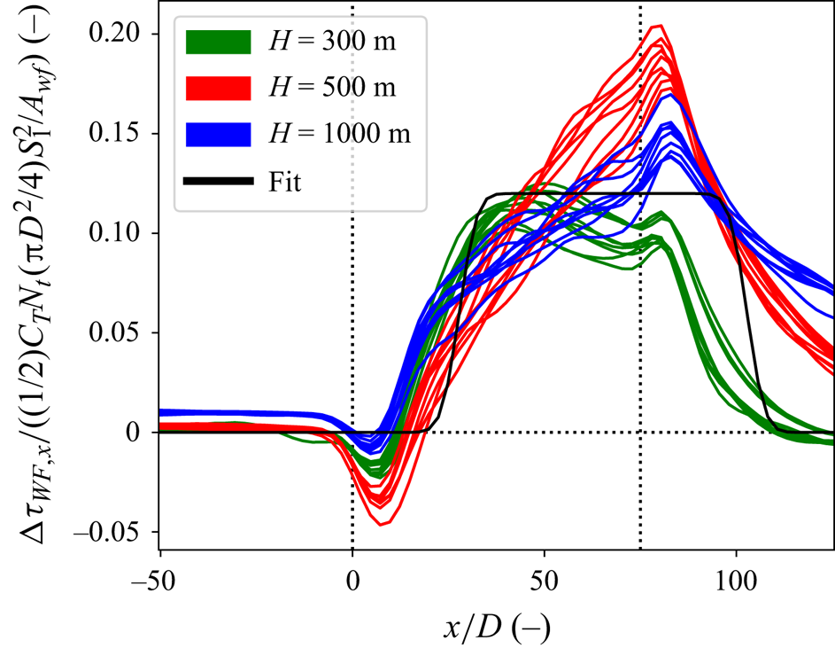
 $\Delta \boldsymbol {\tau }_{{wf}}$ is modelled as a constant added value in the same direction
 $\boldsymbol {e}_t$ as the wind farm forcing. It is assumed to have the same shape as the wind farm, shifted downstream to account for internal boundary layer (IBL) growth. The added term is scaled with the wind farm force density, as is typically done in top-down models for large wind farms (Frandsen Reference Frandsen1992; Calaf et al. Reference Calaf, Meneveau and Meyers2010; Abkar & Porté-Agel Reference Abkar and Porté-Agel2013). The resulting expression for
 $\Delta \boldsymbol {\tau }_{{wf}}$ is
 \begin{equation} \Delta\boldsymbol{\tau}_{{wf}}(x,y) = a_{\tau}\frac{\dfrac{1}{2}C_TN_t \dfrac{{\rm \pi} D^2}{4}\vert\vert\boldsymbol{U}_1\vert\vert^2}{A_{{wf}}} \varPi(\boldsymbol{x}-d_{\tau}D\boldsymbol{e}_1)\boldsymbol{e}_t,\end{equation}
where  $C_T$ and
 $D$ are the average thrust coefficient and turbine diameter of the farm,
 $A_{{wf}}$ is the wind farm area,
 $\boldsymbol {U}_1$ is the unperturbed velocity in the lower layer and
 $\varPi$ is the footprint of the farm, equal to one within the farm and zero everywhere else. The coefficients
 $a_{\tau }$ and
 $d_{\tau }$ are fitted to the LES results of Lanzilao & Meyers (Reference Lanzilao and Meyers2024), and are 0.120 and 27.8, respectively. A description of the fitting procedure can be found in Appendix B. We note that this approach is quite rudimentary, and future work may look into the development of a more involved model.
The horizontal momentum fluxes are modelled with a simple eddy viscosity formulation (Allaerts & Meyers Reference Allaerts and Meyers2019):
 \begin{equation} \bar{\boldsymbol{\tau}}_{hh,1}=\nu_{t,1}\boldsymbol{\nabla}_h\langle\bar{\boldsymbol{u}}_{h}\rangle_{1},\quad \bar{\boldsymbol{\tau}}_{hh,2}=\nu_{t,2}\boldsymbol{\nabla}_h\langle\bar{\boldsymbol{u}}_{h}\rangle_{2},\end{equation}
where  $\nu _{t,1}$ and
 $\nu _{t,2}$ are the depth-averaged eddy viscosities, based on the unperturbed atmospheric state. The increased turbulence near the wind farm is not taken into account in this term.
2.3. Linearized equations
Following Allaerts & Meyers (Reference Allaerts and Meyers2019) we partly linearize the equations (2.7)–(2.10) around a uniform background state  $(\boldsymbol {U}_1,H_1)$ and
 $(\boldsymbol {U}_2,H_2)$ for small perturbations
 $(\boldsymbol {u}^{\prime }_1,\eta _1)$ and
 $(\boldsymbol {u}^{\prime }_2,\eta _2)$ caused by the wind farm forcing. However, since wake effects at the microscale cannot be accurately represented by small perturbations, we keep the wind farm parametrization nonlinear. This results in
 $$\begin{gather} \boldsymbol{U}_1\boldsymbol{\cdot}\boldsymbol{\nabla}_h\eta_1+H_1\boldsymbol{\nabla}_h\boldsymbol{\cdot}\boldsymbol{u}^{\prime}_1=0, \end{gather}$$
 $$\begin{gather}\boldsymbol{U}_2\boldsymbol{\cdot}\boldsymbol{\nabla}_h\eta_2+H_2\boldsymbol{\nabla}_h\boldsymbol{\cdot}\boldsymbol{u}^{\prime}_2=0, \end{gather}$$
 \begin{gather} \boldsymbol{U}_1\boldsymbol{\cdot}\boldsymbol{\nabla}_h\boldsymbol{u}^{\prime}_1 =-\frac{1}{\rho_0}\boldsymbol{\nabla}_h p_t + f_c\boldsymbol{\mathsf{J}}\boldsymbol{\cdot} \boldsymbol{u}^{\prime}_1 + \nu_{t,1}\nabla_h^2\boldsymbol{u}^{\prime}_1 + \frac{\boldsymbol{\mathsf{D}}^{\prime}}{H_1}\boldsymbol{\cdot}\Delta\boldsymbol{u}' - \frac{\boldsymbol{\mathsf{C}}^{\prime}}{H_1}\boldsymbol{\cdot}\boldsymbol{u}^{\prime}_1 \nonumber\\ \quad -\frac{\boldsymbol{T}_{h3,1}-\boldsymbol{T}_{h3,0}}{H_1^2}\eta_1 + (\,\bar{\boldsymbol{f}}_{{wf}}+\overline{\Delta\boldsymbol{\tau}}_{{wf}}) \left(\frac{1}{H_1}-\frac{\eta_1}{H_1^2}\right) + \boldsymbol{\nabla}_h\boldsymbol{\cdot}\langle\boldsymbol{\tau}_{d,hh}\rangle_{1}, \end{gather}
 \begin{gather} \boldsymbol{U}_2\boldsymbol{\cdot}\boldsymbol{\nabla}_h\boldsymbol{u}^{\prime}_2 =-\frac{1}{\rho_0} \boldsymbol{\nabla}_h p_t + f_c\boldsymbol{\mathsf{J}}\boldsymbol{\cdot}\boldsymbol{u}^{\prime}_2 + \nu_{t,2}\nabla_h^2\boldsymbol{u}^{\prime}_2 - \frac{\boldsymbol{\mathsf{D}}^{\prime}}{H_2} \boldsymbol{\cdot}\Delta\boldsymbol{u}^{\prime} \nonumber\\ \quad + \frac{\boldsymbol{T}_{h3,1}}{H_2^2}\eta_2 - \overline{\Delta\boldsymbol{\tau}}_{{wf}}\left(\frac{1}{H_2}-\frac{\eta_2}{H_2^2}\right), \end{gather}
where  $\Delta \boldsymbol {u}'=\boldsymbol {u}^{\prime }_2-\boldsymbol {u}^{\prime }_1$. The matrices
 $\boldsymbol{\mathsf{C}}^{\prime }$ and
 $\boldsymbol{\mathsf{D}}^{\prime }$ are the Jacobians with respect to the velocity perturbations of the turbulent momentum fluxes at the ground and the ABL layer interface, excluding the wind-farm-induced momentum flux, respectively (Allaerts & Meyers Reference Allaerts and Meyers2019). The vectors
 $\boldsymbol {T}_{h3,0}$ and
 $\boldsymbol {T}_{h3,1}$ are the unperturbed momentum fluxes
 $\boldsymbol {\tau }_{h3,0}$ and
 $\boldsymbol {\tau }_{h3,0}$. Note that Allaerts & Meyers (Reference Allaerts and Meyers2019) did not include these terms, which appear in the linearized momentum equations as the derivatives of the net momentum fluxes over the layers with respect to the layer thicknesses
 $h_1$ and
 $h_2$. Physically, this corresponds to the fluxes entering at the layer boundaries being distributed over thicker or thinner layers of fluid. Similarly, the terms containing the wind farm forces and momentum flux also include the derivatives of the layer thicknesses.
In order to easily incorporate the pressure feedback of the internal gravity waves, the model is solved using a Fourier–Galerkin spectral method. This allows all the terms in (2.24)–(2.27) besides the wind-farm-related terms  $\boldsymbol {f}_{{\!wf}}$,
 $\Delta \boldsymbol {\tau }_{{wf}}$ and
 $\langle \boldsymbol {\tau }_{d,hh}\rangle _{1}$ to decouple per wavenumber. To incorporate these wind-farm-related terms, we use a fixed-point iteration solver with a relaxation factor of 0.7. At each step, the decoupled terms form a simple six-by-six matrix for each wavenumber, which is easily solved. The wake model coupling, described in § 3, can then be used to calculate the wind-farm-related terms for the next iteration.
Using a Fourier–Galerkin spectral method imposes periodic boundary conditions on the APM. Any issues related to recycling of the perturbations are avoided by using very large domains of at least 1000 km in the streamwise direction. Finally, we use a grid spacing of  $\Delta x=\Delta y=\ell /2$, following Allaerts & Meyers (Reference Allaerts and Meyers2019).
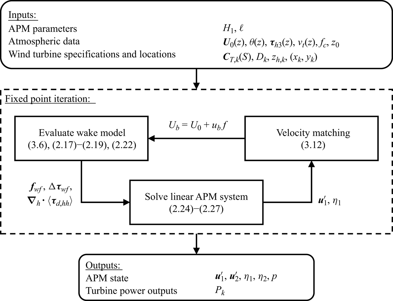
Figure 2 gives an overview of the working of the APM as a whole. The inputs to the APM consist of the choice of  $H_1$ and
 $\ell$, information on the unperturbed atmospheric flow and the wind turbine specification and locations. In a first step, the
 $\theta (z)$ profile is fitted to a CNBL structure using the model by Rampanelli & Zardi (Reference Rampanelli and Zardi2004). Using the resulting
 $H$,
 $g^\prime$ and
 $N_g$, all the coefficients of the linear model can be calculated. Parallel to this, an initial wake model run based on the unperturbed velocity profile
 $U_0(z)$ provides the terms
 $\boldsymbol {f}_{{\!wf}}$,
 $\Delta \boldsymbol {\tau }_{{wf}}$ and
 $\langle \boldsymbol {\tau }_{d,hh}\rangle _{1}$. The iteration procedure described above is then fully set up, and run until converged. The outputs of the APM consist of the mesoscale state
 $\boldsymbol {u}^{\prime }_1$,
 $\eta _1$,
 $\boldsymbol {u}^{\prime }_2$,
 $\eta _2$ and
 $p$, and the turbine power outputs
 $P_k$.
Flowchart showing the inputs, outputs and solving procedure of the APM. The inputs and outputs are indicated by the rounded boxes. The arrows show the flow of information. The subscript  $k$ indicates turbine-specific variables.

2.4. Momentum budget analysis
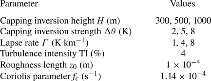
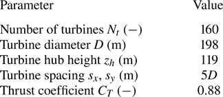
To investigate the importance of each of the terms in (2.9) and (2.10), we perform a momentum budget analysis using the LES results of Lanzilao & Meyers (Reference Lanzilao and Meyers2024). This is a dataset of 40 simulations of the same large wind farm of  $N_t=160$ IEA 10 MW turbines (Bortolotti et al. Reference Bortolotti, Tarres, Dykes, Merz, Sethuraman, Verelst and Zahle2019), arranged in a staggered layout with 16 rows and 10 columns (Lanzilao & Meyers Reference Lanzilao and Meyers2023a). From these, we analyse 27 CNBL simulations, leaving out the cases with low capping inversions or no stratification. The remaining cases all have different combinations of boundary layer heights, capping inversion strengths and atmospheric stratification levels. An overview of the atmospheric states and the wind farm can be found in tables 1 and 2, respectively. We follow the naming convention of Lanzilao & Meyers (Reference Lanzilao and Meyers2024), where cases are characterized by the boundary layer height, capping inversion strength and atmospheric lapse rate. For instance, the case with
 $H=500\ \mathrm {m}$,
 $\Delta \theta =5\ \mathrm {K}$ and
 $\varGamma =4\ \mathrm {K}\ \mathrm {km}^{-1}$ is denoted as H500-
 $\Delta \theta$5-
 $\varGamma$4. Note that these values correspond to the initial conditions, and the exact profiles have changed slightly during the precursor spin-up (see Lanzilao & Meyers (Reference Lanzilao and Meyers2024) for details).
Overview of the atmospheric conditions of the flow cases from Lanzilao & Meyers (Reference Lanzilao and Meyers2024) used for the validation of the coupling method and the APM. In total all 27 combinations of these parameters are considered. The TI value is taken at the turbine hub height of 119 m. Note that these values correspond to the initial profiles, and that the actual conditions changed slightly during the precursor spin-up. See Lanzilao & Meyers (Reference Lanzilao and Meyers2024) for a detailed description of the simulations.

Description of the wind farm from Lanzilao & Meyers (Reference Lanzilao and Meyers2024) used for the validation of the coupling method and the APM.

To analyse the momentum budget for the APM, we construct an APM ground truth from the LES data. This is done by applying the filtering and height-averaging operations defined in § 2 to the LES flow fields numerically. In a first step, the velocity and pressure fields are Gaussian-filtered in the horizontal direction with the APM filter length. Then,  $z_1$ is obtained by advecting a set of points over the domain starting from height
 $z=H_1$, to obtain the surface separating the two ABL layers. We initialize these points to coincide with the LES grid along the domain inlet, resulting in 1380 points with a regular spacing of 21.7 m. We find capping inversion displacement by applying the Rampanelli & Zardi (Reference Rampanelli and Zardi2004) model, and Gaussian-filtering the results. Finally, the velocities and pressure are height-averaged between the layer boundaries. The pressure perturbation at the top of the ABL
 $p_t$ is evaluated 50 m below the bottom of the capping inversion, to ensure that it is not partly evaluated within the inversion if the fitting by the Rampanelli & Zardi (Reference Rampanelli and Zardi2004) model is poor.
We now consider the momentum balance in the streamwise direction, denoted by  $x$, across the wind farm. At each position, we evaluate the momentum balance across the lateral cross-section of the wind farm, using an infinitesimally thin domain with the wind farm width
 $W$ and length
 ${{\rm d}{\kern0.8pt}x}$. Note that we perform this analysis on the APM momentum equations, which also implies a horizontal filtering and height-averaging of the flow. After subtracting the background momentum balance between the Coriolis force, vertical momentum flux and geostrophic pressure gradient of the precursor simulation, the momentum budget equation in the lower layer becomes
 \begin{align} & \underbrace{-\int_0^{W}{\langle\bar{\boldsymbol{u}}_h\rangle_{1}\boldsymbol{\cdot} \boldsymbol{\nabla}_h\langle\bar{u}_h\rangle_{1}\,\mathrm{d}y}}_{\mathcal{F}_{u,1}} \underbrace{-\int_0^{W}{\frac{1}{\rho_0}\frac{\partial\langle\,\bar{p}\rangle_1}{\partial x}\mathrm{d}y}}_{\mathcal{F}_{p,1}} + \underbrace{\int_0^{W}{f_c v_{1}^{\prime}\,\mathrm{d}y}}_{\mathcal{F}_{C,1}} \nonumber\\ &\quad + \underbrace{\int_0^{W}{\langle\bar{\tau}_{xx}\rangle_{1}\mathrm{d}y} + \langle\bar{\tau}_{xy}\rangle_{1}\vert^{W}_{0} + \int_0^{W}{\left(\frac{\bar{\tau}_{3x,1}-\bar{\tau}_{3x,0}}{h_1} - \frac{T_{3x,1}-T_{3x,0}}{H_1}\right)\mathrm{d}y}}_{\mathcal{F}_{\tau,1}} \nonumber\\ &\quad +\underbrace{\int_0^{W}{\frac{\bar{f}_{{wf},x}}{h_1}\mathrm{d}y}}_{\mathcal{F}_{t}} +\underbrace{\int_0^{W}{\langle\boldsymbol{\nabla}\boldsymbol{\cdot}(\boldsymbol{\tau}_{d,x})\rangle_1\,\mathrm{d}y}+ \int_0^{W}{\frac{1}{h_1}\boldsymbol{\nabla}_h\boldsymbol{\cdot}(h_1\langle\bar{\boldsymbol{u}}_{h,1}^{\prime\prime\prime} \bar{u}_{x,1}^{\prime\prime\prime}\rangle_1)\,\mathrm{d}y}}_{\mathcal{F}_{sg,1}} \nonumber\\ &\quad +\underbrace{\int_0^{W}{\frac{\mathcal{R}_{x,1}}{h_1}\mathrm{d}y}}_{\mathscr{R}_{1}} = 0. \end{align}
The terms in the above equation represent the advection of momentum ( $\mathcal {F}_{u}$), the pressure gradient (
 $\mathcal {F}_{p}$), the Coriolis force (
 $\mathcal {F}_{C}$), the turbulent momentum fluxes (
 $\mathcal {F}_{\tau }$), the turbine thrust forces (
 $\mathcal {F}_{t}$), the subgrid terms (
 $\mathcal {F}_{sg}$) and the residual term (
 $\mathscr {R}$). For the upper layer, the result is analogous, but there is only a momentum flux at the bottom of the layer, and there is no wind farm thrust contribution. The above equation is the complete momentum budget, without any parametrizations or linearization.
We now calculate these terms from the LES results of Lanzilao & Meyers (Reference Lanzilao and Meyers2024). In § 2.4.1, we discuss their calculation from (2.28), in order to get insight into which effects are important to mesoscale wind farm flows. Afterwards, in § 2.4.1 we discuss applying the parametrizations described in § 2.2 to the LES-based APM states, so that these parametrizations can be validated a priori. Both results are shown together in figure 3.
Streamwise variation of all the terms in the momentum budget in the lower (a) and upper (b) layers. All the terms are scaled with  $W\vert \vert \boldsymbol {U}_1\vert \vert ^2/L$ and
 $W\vert \vert \boldsymbol {U}_2\vert \vert ^2/L$ in the lower and upper layers, respectively, where
 $L$ is the farm length. The solid lines are the terms as calculated from the LES data and the dashed lines are the parametrized and linearized versions calculated from the LES-based APM state. The vertical dotted lines indicate the wind farm region.

2.4.1. The LES data analysis
We now evaluate the momentum budget for the case H500- $\Delta \theta$5-
 $\varGamma$4. It has a Froude number of approximately 1, with internal waves strong enough to prevent the choking effect described by Smith (Reference Smith2010). There are weak resonant lee waves that cause velocity variations throughout the farm, and there is a moderate blockage effect.
Figure 3 (solid lines) shows the streamwise momentum balance through the farm. Both the lower and upper layers are shown, and there are substantial differences in the flow dynamics. In the lower layer, the turbine forces are felt directly, and they are balanced primarily by the convective deceleration, the pressure gradients, the subgrid forces and the turbulent momentum fluxes. While the wind farm force is relatively constant throughout the farm, the other terms vary strongly, and which term is most important can change depending on the location. Upstream, the only active terms are the unfavourable pressure gradient and the flow deceleration. At the farm entrance, the pressure gradient becomes smaller, as the pressure perturbation reaches its maximum, and the turbine forces are completely balanced by the flow deceleration and the dispersive stresses. The rise in the dispersive velocity contributions is to be expected, as within the farm the turbine wakes form a strongly heterogeneous flow field with variations below the filter length of  $\ell =1\ \mathrm {km}$.
Recently, Bastankhah et al. (Reference Bastankhah, Mohammadi, Lees, Diaz, Buxton and Ivanell2024) also found that dispersive stresses played an important role in the momentum balance in wind farm flows. However, they only averaged in the lateral direction, and found the terms to contribute at turbine-length scales in the streamwise direction. In contrast, we find that when the flow is filtered in the streamwise direction as well, the main contribution of this term occurs at the start of the farm as the flow heterogeneity is rapidly established, similar to sparse canopy flows (Moltchanov et al. Reference Moltchanov, Bohbot-Raviv and Shavit2011). Throughout the farm, the dispersive stresses diminish slowly as the wake mixing increases, so that their divergence at the farm exit is not as strong as their rise at the entrance. Overall, we conclude that these dispersive stresses are important to take into account when parametrizing wind farms in the APM, as their maximum effect at the farm entrance is as strong as that of the pressure gradient.
Further downstream, the wind farm forcing is mostly counteracted by the flow acceleration, the pressure gradient and the turbulent momentum fluxes, which primarily consist of the vertical flux contributions. Across the farm, the pressure gradient is favourable, while the turbulent momentum fluxes slowly increase. As a result, the flow gradually decelerates less throughout the farm, with the velocity reaching a roughly constant value towards the end of the farm and increasing again in the farm wake. On top of these average trends, the pressure gradient and flow convection also show strong oscillations throughout the farm, which balance each other. These are the resonant lee waves described by Allaerts & Meyers (Reference Allaerts and Meyers2019).
In the upper layer, the momentum balance is simpler. The main contributions are from the oscillations in the pressure gradient and the flow acceleration, as the resonant lee waves excite the whole ABL. On top of that, the turbulent momentum flux, which prevented flow deceleration and helped wake recovery in the lower layer, now slows down the flow, although it is largely counteracted by the favourable pressure gradient within the farm.
Finally, we note that the Coriolis contribution  $\mathcal {F}_{C}$ is small compared with the terms discussed above. The only smaller term is the residual
 $\mathscr {R}$.
2.4.2. The APM approximations
We now verify the correctness of the approximations made when linearizing and parametrizing the various terms in the APM. To this end, the dashed lines in figure 3 show the momentum budget analysis of (2.26)–(2.27). Note that this is obtained without running the APM, and instead computed using the LES-based APM state. The convective terms are linearized, the height-averaged pressure has been replaced with the pressure at the top of the ABL  $p_t$ and the turbulent momentum fluxes are calculated using the linearized versions of (2.20), (2.21) and (2.23a,b). The wind farm forces and dispersive stresses are evaluated using the wake model, coupled to the LES-based APM state (see § 3 for details of the wake model coupling). The background state has been computed using the precursor velocity and potential temperature profiles.
Overall, the APM parametrizations perform well. In all terms, the general trends are captured. The pressure gradient is matched very well by using  $p_t$ instead of
 $p_1$ and
 $p_2$, indicating that the pressure perturbations are dominated by the gravity waves in the free atmosphere. This hydrostatic approximation is worse for the
 $H=1\ \mathrm {km}$ cases (not shown), but still holds there as well.
The errors in the  $\mathcal {F}_{\tau }$ terms are larger, which is to be expected given the basic turbulence parametrization used in this work. The APM overestimates the vertical momentum flux at the farm entrance, where there is a velocity difference between the APM layers but the growing IBL has not yet reached
 $z_1$, and underestimates the horizontal momentum flux at the farm boundaries. Additionally, the vertical momentum fluxes at the ground and at
 $h_1$ are respectively over- and underestimated within the farm. For
 $\bar {\tau }_{3x,0}$, this is mainly due to the lack of correction for the presence of the wind farm, whereas for
 $\bar {\tau }_{3x,1}$ it is mostly caused by the linearization. For the lower layer, where both contribute to
 $\mathcal {F}_{\tau }$, these errors cancel out, but for the upper layer the result is an underestimation of
 $\mathcal {F}_{\tau }$. The simple parametrization used here can be improved upon in future work (Stipa et al. Reference Stipa, Allaerts and Brinkerhoff2024b).
Additionally, the subgrid terms are underestimated at the farm entrance. This is mostly due to an underestimation of the dispersive stresses, while the Taylor-shear dispersion has only a minor impact.
Finally, the main discrepancy comes from the linearization of the convective terms. As the mesoscale velocity drops, the flow deceleration is overestimated by a factor of  $U_1/\langle \bar {u}\rangle _1$. With flow perturbations of roughly
 $u_1^{\prime }/U_1\approx 0.25$, this mismatch can be severe.
3. Wake-model coupling
This section describes the wake model used in this work, and the new method for coupling it to the APM.
3.1. Wake model
To incorporate the spatially varying effects of gravity waves, the wake model should be able to handle heterogeneous background velocities. We therefore employ the wake-merging method of Lanzilao & Meyers (Reference Lanzilao and Meyers2021a). This superposition method conserves mass and momentum as long as the background flow variations have large length scales, which should be the case for gravity-wave-induced perturbations. Each turbine multiplies the flow by a wake modifier, so that every turbine wake has a self-similar behaviour with respect to the flow without it. For two-directional flow, Lanzilao & Meyers (Reference Lanzilao and Meyers2021a) gave a recursive formula:
 $$\begin{gather} \boldsymbol{u}_k(\boldsymbol{x}) = (\boldsymbol{u}_{k-1}(\boldsymbol{x}) \boldsymbol{\cdot}\boldsymbol{e}_{{\perp},k})(1-W_k(\boldsymbol{x}))\boldsymbol{e}_{{\perp},k} + (\boldsymbol{u}_{k-1}(\boldsymbol{x})\boldsymbol{\cdot}\boldsymbol{e}_{{\parallel},k}) \boldsymbol{e}_{{\parallel},k} \quad k=1,\ldots,N_t, \end{gather}$$
 $$\begin{gather}\boldsymbol{u}_w(\boldsymbol{x}) = \boldsymbol{u}_{N_t}(\boldsymbol{x}), \qquad \boldsymbol{u}_0(\boldsymbol{x}) = \boldsymbol{U}_b, \end{gather}$$
where  $N_t$ is the number of turbines and
 $W_k$ is the wake deficit function of turbine
 $k$, defined along the background flow streamlines. The turbines are ordered upstream to downstream, so that the first turbine applies its wake to the background velocity
 $\boldsymbol {U}_b$. The unit vectors
 $\boldsymbol {e}_{\perp,k}$ and
 $\boldsymbol {e}_{\parallel,k}$ denote the directions perpendicular and parallel to the rotor disk of turbine
 $k$ (see Lanzilao & Meyers (Reference Lanzilao and Meyers2021a) for details).
For the wake-model coupling method developed later, it will be important to have an explicit expression for the final velocity field  $\boldsymbol {u}_w$. This can be obtained by rewriting equations (3.1) as a matrix multiplication with
 $\boldsymbol {u}_{k-1}$:
 \begin{equation} \boldsymbol{u}_k(\boldsymbol{x}) = \boldsymbol{\mathsf{A}}_k(\boldsymbol{x}) \boldsymbol{\cdot}\boldsymbol{u}_{k-1}(\boldsymbol{x}) \quad k=1,\ldots,N_t, \end{equation}
where
 \begin{equation} \boldsymbol{\mathsf{A}}_k(\boldsymbol{x}) = (1-W_k(\boldsymbol{x})) (\boldsymbol{e}_{{\perp},k}\boldsymbol{e}_{{\perp},k}) + (\boldsymbol{e}_{{\parallel},k} \boldsymbol{e}_{{\parallel},k}). \end{equation}
The explicit formula for two-directional flow is then
 \begin{equation} \boldsymbol{u}_w(\boldsymbol{x}) = \prod_{k=1}^{N_t}\boldsymbol{\mathsf{A}}_k(\boldsymbol{x}) \boldsymbol{\cdot}\boldsymbol{U}_{b}(\boldsymbol{x}). \end{equation}
For simplicity, this paper neglects multi-directional effects and assumes straight streamlines throughout the farm along the direction of the background flow and the wind farm force  $\boldsymbol {e}_t$. Throughout this section, all velocities refer to the velocity components in this direction, unless stated otherwise. An extension of the coupling method to two-directional flow is possible using (3.5), but beyond the scope of this work. For a given background velocity
 $U_b$, the wake model then predicts the following velocity field
 $u_{w}$ (Lanzilao & Meyers Reference Lanzilao and Meyers2021a):
 \begin{equation} u_{w}(x,y,z)=U_b(x,y,z)\prod_{k=1}^{N_t}[1-W_k(x,y,z)]. \end{equation}
For the wake deficit function, we use the Gaussian wake model of Bastankhah & Porté-Agel (Reference Bastankhah and Porté-Agel2014). The evolution of the turbulence intensity is incorporated using the model of Niayifar & Porté-Agel (Reference Niayifar and Porté-Agel2016). The wake model is not tuned, and instead uses the parameters given in the papers cited above, as these have been found to perform well when compared with operational data (Doekemeijer, Simley & Fleming Reference Doekemeijer, Simley and Fleming2022). The turbines are mirrored to account for ground effects.
Additionally, an induction-zone model is included to accurately represent the velocity field upstream of the turbine. In this work, we use the model by Troldborg & Meyer Forsting (Reference Troldborg and Meyer Forsting2017) with the parameters reported in Branlard et al. (Reference Branlard, Quon, Meyer Forsting, King and Moriarty2020). The induction model is only used to better represent the velocity field for the coupling method, and is not used when calculating the turbine inflow velocities for the calculation of thrust and power. The necessity of the induction model is discussed in depth in § 4.1.1.
3.2. Velocity matching
The goal of the wake model coupling is to find a background velocity  $U_b$ based on a mesoscale APM state. This is done by ensuring that the velocity fields predicted by the wake model and the APM are consistent with each other. Concretely, height-averaging and filtering the wake model velocity as in (2.5) and (2.1) should result in the APM's lower-layer velocity field. For a given mesoscale state, the goal is thus to find a heterogeneous background velocity that, once wakes are superimposed on it, matches the mesoscale velocity. This requires the following equation to hold:
 \begin{equation} \frac{1}{z_1}\int_{0}^{z_1}{\iint_{L_x \times L_y}{G_\ell(x-x^{\prime},y-y^{\prime}) u_{w}(x^{\prime},y^{\prime},z)}\,\mathrm{d}\kern0.06em x^{\prime}\,\mathrm{d}y^{\prime}}\,\mathrm{d}z = \langle\bar{u}\rangle_{1}, \end{equation}
where  $\langle \bar {u}\rangle _{1}$ is the mesoscale velocity in the lower layer along
 $\boldsymbol {e}_t$ and
 $L_x \times L_y$ is the size of the APM domain. If the background velocity
 $U_b$ results in a wake-model velocity that satisfies (3.7), the velocity fields of the APM and the wake model are consistent. Because of this concept, we refer to the coupling method developed here as velocity matching (VM).
Equation (3.7) matches the velocity fields over the entire computational domain. However, it is unnecessary and computationally costly to obtain the background velocity in regions far away from the farm. We therefore split the velocity into the parts inside and outside the wind farm:
 \begin{equation} u_{w}(x,y,z) \approx U_b(x,y,z)\prod_{k=1}^{N_t}[1-W_k(x,y,z)]\delta_{{wf}}(x,y) + \langle\bar{u}\rangle_{1}(x,y)(1-\delta_{{wf}}(x,y)), \end{equation}
where  $\delta _{{wf}}=1$ in a region
 $\varOmega _{{wf}}$ around the wind farm and
 $\delta _{{wf}}=0$ everywhere else. In the latter area, we assume it is roughly equal to the mesoscale velocity, which should be a good approximation far away from the farm. The boundaries of
 $\varOmega _{{wf}}$ are placed at a distance of at least
 $2\ell$ from the farm edges. The equation for the background velocity then becomes
 \begin{align} & \frac{1}{z_1}\int_{0}^{z_1}{\iint_{\varOmega_{{wf}}}{G_\ell(x-x^{\prime},y-y^{\prime}) U_b(x^{\prime},y^{\prime},z)\prod_{k=1}^{N_t} [1-W_k(x^{\prime},y^{\prime},z)]}\,\mathrm{d}\kern0.06em x^{\prime}\,{{\rm d}y}^{\prime}}\,\mathrm{d}z \nonumber\\ &\quad =\langle\bar{u}\rangle_{1}(x,y)-\iint_{L_x \times L_y}{G_\ell(x-x^{\prime},y-y^{\prime}) \langle\bar{u}\rangle_{1}(x^{\prime},y^{\prime})(1-\delta_{{wf}}(x^{\prime},y^{\prime}))}\,\mathrm{d}\kern0.06em x^{\prime}\,\mathrm{d}y^{\prime}. \end{align}
Finally, to avoid having to solve for the three-dimensional background velocity, we decompose  $U_b$ into an unperturbed state
 $U_{0}(z)$, which is known as an input to the APM, and a perturbation:
 \begin{equation} U_b(x,y,z) = U_{0}(z) + u_b(x,y)f(z). \end{equation}
We use a standard logarithmic shape function for  $f$:
 \begin{equation} f(z) = \frac{1}{\kappa}\log{\left(\frac{z}{z_0}\right)}, \end{equation}
where  $\kappa =0.41$ is the Von Kármán constant and
 $z_0$ is the roughness length. The resulting final VM equation for the background velocity scale
 $u_b$ is then
 \begin{align} & \frac{1}{z_1}\int_{0}^{z_1}{\iint_{\varOmega_{{wf}}}G_\ell(x-x^{\prime},y-y^{\prime}) u_b(x^{\prime},y^{\prime})f(z)\prod_{k=1}^{N_t}[1-W_k(x^{\prime},y^{\prime},z)]\,\mathrm{d}\kern0.06em x^{\prime}\,\mathrm{d}y^{\prime}\,\mathrm{d}z} \nonumber\\ &\quad =\langle\bar{u}\rangle_{1}(x,y) \nonumber\\ &\qquad -\iint_{L_x \times L_y}{G_\ell(x-x^{\prime},y-y^{\prime}) \langle\bar{u}\rangle_{1}(x^{\prime},y^{\prime},z)(1-\delta_{{wf}}(x^{\prime},y^{\prime}))}\,\mathrm{d}\kern0.06em x^{\prime}\,\mathrm{d}y^{\prime} \nonumber\\ &\qquad -\frac{1}{z_1}\int_{0}^{z_1}{\iint_{\varOmega_{{wf}}}{G_\ell(x-x^{\prime},y-y^{\prime})U_0(z) \prod_{k=1}^{N_t}[1-W_k(x^{\prime},y^{\prime},z)]}\,\mathrm{d}\kern0.06em x^{\prime}\,\mathrm{d}y^{\prime}}\,\mathrm{d}z. \end{align}
Equation (3.12) is a linear equation for the background velocity, which, once solved for, can be used as an input for the wake model. As this essentially requires inverting a filtering operation, the problem is ill-posed. We avoid this issue by phrasing it as a least-squares problem, and limiting the number of degrees of freedom of the background velocity. Appendix C provides a detailed overview of this procedure.
4. The LES-based validation
This section contains a validation study of the VM method and the APM based on LES data. Section 4.1 contains an a priori validation of the coupling method. Section 4.2 performs an a posteriori validation campaign of the full APM.
4.1. The VM method validation
To validate the VM method derived in the previous section, we need APM states for it to couple to. In the current section, we do not yet use the APM for this, but instead use the LES-based states set up for the momentum budget analysis in § 2.4. This allows us to test the coupling's performance separately from the APM.
Section 4.1.1 discusses the dependence of the VM method on the performance of the wake model. Section 4.1.2 validates the coupling using the LES simulations outlined above.
4.1.1. Importance of wake-model performance
For the VM method to perform well, the wake model needs to provide good estimates for the velocity field. Typically, wake models only need to be accurate near downstream turbines, as the velocity in other regions, such as the near-wake or the induction region, does not affect the inflow velocities for other turbines. As a result, a wake model with an unrealistic near-wake flow field can still perform well, especially when tuned. However, when the VM method couples such a wake model to a mesoscale state, it will try to correct the errors made in the global velocity field, thereby worsening the power prediction. To prevent this, we make three choices when setting up the wake model. First, we mirror the turbines to account for ground effects. Second, we apply a correction to the centreline velocity deficit in the near-wake region (Zong & Porté-Agel Reference Zong and Porté-Agel2020). Third, we include an induction model to account for upstream velocity changes. Here, we use the model by Troldborg & Meyer Forsting (Reference Troldborg and Meyer Forsting2017), but other models should also achieve similar performance (Branlard et al. Reference Branlard, Quon, Meyer Forsting, King and Moriarty2020). Note that this induction model is only used to estimate the velocity fields in (3.12), and not when performing thrust and power calculations. In the latter it is not necessary, as wake models are designed to yield predictions for these properties. In order to investigate this dependence on the wake model in detail, we analyse the VM method's performance for the case H500- $\Delta \theta$0-
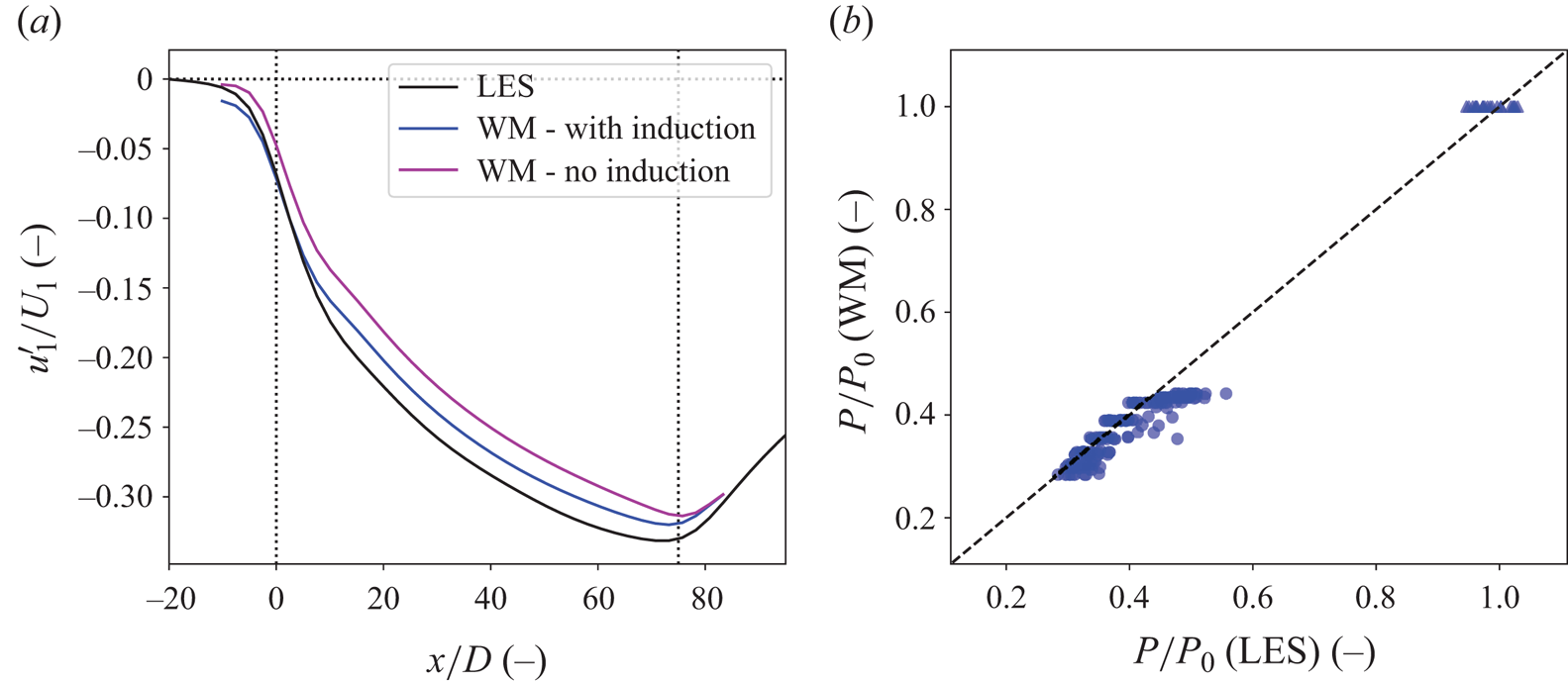
 $\varGamma$0. This is a purely neutral case, without gravity waves and minimal mesoscale feedback effects. As a result, one would expect an uncoupled wake model to perform well in terms of both velocity and power, and for the coupling method to predict a background velocity perturbation close to zero. Figure 4 shows the mesoscale velocity deficits
 $\boldsymbol {u}^{\prime }_1$ and the power output of the turbines as found by LES and an uncoupled wake model, both with and without induction. The wake model background velocity is simply the precursor profile
 $U_0(z)$. The LES turbine power outputs were scaled with the power output for a single turbine, and the wake-model power outputs are scaled with the power calculation for a single turbine with the precursor as inflow conditions. Note that even without an induction model, there is a mesoscale velocity deficit upstream of the farm, as the Gaussian filtering operation smears out the turbine wakes within the farm. We observe that the wake model reproduces both the velocity and power accurately, with an average power error across all turbines of 1.8 %. However, without an induction model, the wake model underestimates the velocity upstream of and throughout the farm.
Performance of the wake model (WM) for the case H500- $\Delta \theta$0-
 $\varGamma$0. (a) The mesoscale velocity deficit as found by LES (black) and the wake model, both with and without induction model (blue and magenta, respectively). The dotted lines denote the wind farm region. (b) The power output as found by LES (
 $x$ axis) and wake model (
 $y$ axis). The triangles and the circles denote the first two turbine rows and the remainder of the farm, respectively.

We now apply the VM method to this case, matching the wake-model velocities to the LES-based APM state. Figure 5 shows the resulting background velocity perturbations  $u_b$ with and without using an induction model. When an induction model is used, the VM method predicts almost no variations in the background velocity. Without, the coupling lowers the background velocity considerably. We find that power predictions of the wake model based on this background velocity are up to 10 % too low.
Background velocity perturbations  $u_b$ as found by applying the VM method to the LES-based APM state for the case H500-
 $\Delta \theta$0-
 $\varGamma$0 when using a wake model with an induction model (a) and without an induction model (b). The black lines indicate the turbine disks.

We conclude that the performance of the wake model drastically affects the VM method's output, and good results depend on the estimations of the turbine-level velocities being realistic at every point in the farm. This requires the wake model to account for turbine induction, the near-wake region and ground effects. With the corrections used in this work, this is achieved fairly well, although there is still a slight underestimation of the mesoscale velocity deficit within the farm.
4.1.2. Coupling performance
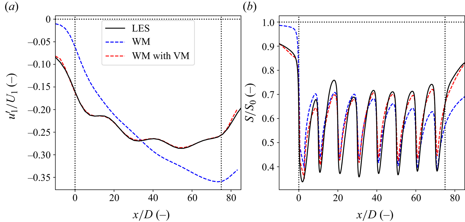
We coupled the wake model to the LES-based APM state for all 27 simulations with atmospheric stratification. As a comparison, we also apply the uncoupled wake model to all analysed cases. The coupling method was consistently able to provide background velocities that resulted in matching mesoscale velocity fields. Figure 6 shows this for the case H500- $\Delta \theta$5-
 $\varGamma$4, which is the same case as shown in § 2.4. It is clear that this required significant corrections to the background velocity of the wake model, as the uncoupled wake model has a very different profile. Moreover, this mesoscale matching corresponds to a better agreement of the velocity fields on the turbine level. Figure 6(b) shows the local velocity averaged over a streamwise tube with the turbine diameter, placed at hub height through the centre of the farm, for the same case. The velocity-matched wake model captures well the lower velocity at the farm entrance, and follows the LES state throughout the rest of the farm. This good performance is consistent across all tested cases.
Streamwise velocity deficits through the centre of the farm of the LES (solid lines, black) and the wake model (dashed lines), both uncoupled and coupled (blue and red, respectively), for the case H500- $\Delta \theta$5-
 $\varGamma$4. (a) The mesoscale velocity deficit. (b) The average velocity across a tube with the turbine diameter. The dotted lines denote the wind farm region.

For all cases, there is a blockage effect, resulting in a lower background velocity at the start of the farm. Throughout the farm itself, the wake model background speeds  $U_b$ increase, and even become larger than the unperturbed speeds
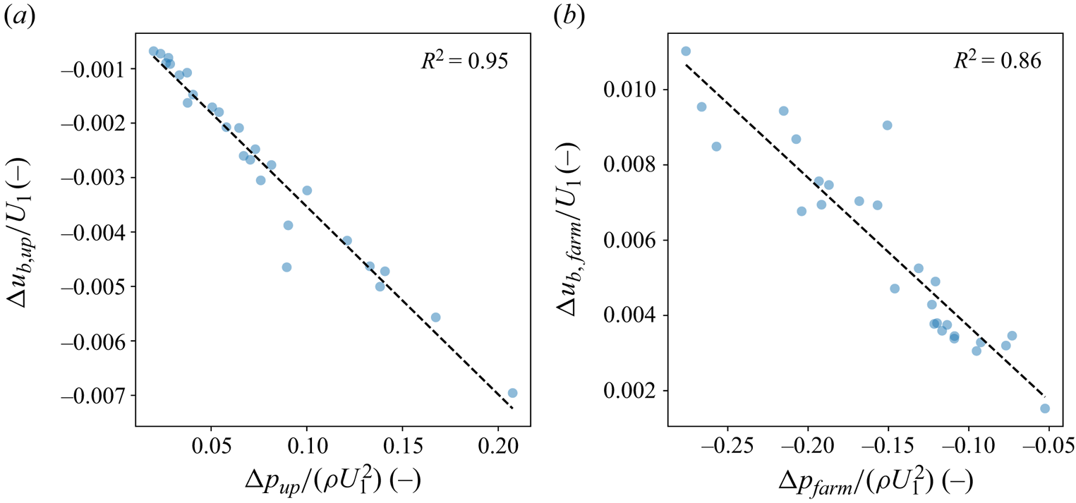
 $U_0$ halfway through the farm. This is consistent with the pressure gradients, which Lanzilao & Meyers (Reference Lanzilao and Meyers2024) found to be unfavourable upstream of the farm, and favourable throughout. To better quantify this relation, we define the following metrics:
 $$\begin{gather} \Delta u_{b,up}=\int_0^{W}{u_b(0,y)\,\mathrm{d}y}, \end{gather}$$
 $$\begin{gather}\Delta p_{up}=\int_0^{W}{p(0,y)\,\mathrm{d}y}, \end{gather}$$
 $$\begin{gather}\Delta u_{b,farm}=\int_0^{W}{(u_b(L,y)-u_b(0,y))\,\mathrm{d}y}, \end{gather}$$
 $$\begin{gather}\Delta p_{farm}=\int_0^{W}{(\,p(L,y)-p(0,y))\,\mathrm{d}y}, \end{gather}$$
where  $W$ and
 $L$ are the farm width and length, respectively, so that the variables above describe the averaged velocity and pressure perturbations at the entrance of the farm (4.1)–(4.2) and their difference across it (4.3)–(4.4). Figure 7(a) shows that the upstream unfavourable pressure rise correlates very well with the upstream change of background velocity. Likewise, figure 7(b) shows that the favourable pressure drop over the farm correlates very well with the change in background velocity in the farm. Thus the VM method manages to catch the expected favourable and unfavourable pressure gradients through
 $u_b$.
The averaged pressure (horizontal axes) and background velocity perturbations (vertical axes) over the width of the farm, evaluated at the farm entrance (a) and their difference across the farm (b). The dashed lines show linear regressions, with the  $R^2$ values as the coefficient of determination.

We also compare the turbine power outputs for all flow cases. The results are shown in figure 8. The coupled wake model significantly outperforms the uncoupled wake model. The power output of the front-row turbines is retrieved very well, with the VM method having an average error across all front turbines of 1 %, compared with 24 % for the uncoupled wake model. This shows that the coupling correctly captures the blockage effect in the mesoscale velocity fields. It also has lower errors throughout the farm when compared with the uncoupled wake model, as it takes into account the positive effect of the favourable pressure gradient in the farm. That said, it still underestimates farm power output, with the largest errors situated between the second and fifth turbine rows (see figure 8b). This is probably primarily caused by a combination of two factors. First, wake deflection, which occurs in the farm entrance region under strong stratification conditions, will cause some turbines to not be waked in the studied farm layout. As we simplify the wake model to be unidirectional in this work, we do not capture this effect. However, this is not an inherent limitation of the VM method, as it can be extended to two-directional flow using the formulation of the wake model outlined in § 3. Figure 8(b) shows that the largest errors are predicted for the turbines in the entrance region at the side of the farm, which are the turbines that are most affected by upstream wake deflection. Second, as can be seen in figure 4(a), the wake model slightly overestimates the velocity throughout the farm. As discussed in the previous section, the VM method depends on the performance of the wake model, so more realistic wake models could improve the results. Future work should address both of these issues.
(a) The turbine power outputs for all cases for both the uncoupled (blue) and coupled (red) wake model as compared to the LES. The triangles and the circles denote the first two turbine rows and the remainder of the farm, respectively. (b) The average power output error of the VM method for each turbine in the farm.

We conclude that the VM coupling method performs very well. It reproduces the mesoscale flow throughout the farm, which also results in a better approximation of the local flow. Furthermore, this translates to a better capturing of the turbine power outputs, especially for the front-row turbines. This good performance was consistent across all analysed flow cases.
4.2. The APM validation
The APM is validated using the same LES data from Lanzilao & Meyers (Reference Lanzilao and Meyers2024) as in the previous sections. To do this, the APM was run for each of the flow cases listed in table 1 with the wind farm described in table 2. For each flow case, the background ABL state around which the APM is linearized was based on the corresponding precursor simulation. As the APM does not have a fringe region, the periodic boundary conditions of the Fourier spectral method were dealt with by using a domain length of  $L_x=10\,000\ \mathrm{km}$. We use the same domain width of
 $L_y=30\ \mathrm {km}$, with the same periodic boundary conditions as the LES.
Section 4.2.1 discusses the flow fields generated by the APM and its performance in capturing the mesoscale wind farm effects. Section 4.2.2 investigates the power output predictions made by the APM.
4.2.1. Flow physics
To analyse the flow states produced by the APM, we take an in-depth look at the H500- $\Delta \theta$5-
 $\varGamma$4 case from Lanzilao & Meyers (Reference Lanzilao and Meyers2024), which was also discussed in the previous sections. Both the flow physics and the APM performance are representative of the total dataset. We both provide a qualitative description of the flow phenomena and indicate the strengths and shortcomings of the APM.
To qualitatively compare the output of the APM against the LES, figure 9 shows the streamwise cross-sections of the flow through the centre of the farm. The capping inversion separating the ABL from the free atmosphere is clearly visible. The displacement of this capping inversion triggers internal gravity waves in the free atmosphere above it, and these along with the pressure feedback from the inversion displacement itself cause a significant velocity reduction upstream of the farm. The gravity waves within the free atmosphere are captured fairly well up to 5 km. Within the ABL, the resonant lee waves described by Allaerts & Meyers (Reference Allaerts and Meyers2019) are visible, especially above the IBL forming above the wind farm. Notably, the APM states do not capture this IBL, as it only contains the height-averaged flow within the layers. While the APM models the flow upstream and throughout the farm fairly well, it does not accurately represent the farm wake structure. This is to be expected, due to its inability to model IBL growth and limited turbulence parametrization. Despite these shortcomings, the comparison shows decent agreement between the APM and LES, especially for the stratification-related flow features.
(a) Cross-section through the centre of the farm of the velocity perturbation for the case H500- $\Delta \theta$5-
 $\varGamma$4, as found by LES. Cross-section through the centre of the farm of the velocity perturbation for the APM state based on the LES results (b) and as found by the APM (c) for the case H500-
 $\Delta \theta$5-
 $\varGamma$4. The solid black lines denote the pliant surfaces separating the APM layers while the dashed lines show the wind farm region. The flow above the capping inversion is found using linear gravity wave theory.

Continuing this qualitative discussion, figure 10 shows the top view of the  $u_1^{\prime }$ perturbation velocity for both the APM and the LES-based state. Once again, the blockage effect in front of the farm is clearly seen. From this top view, the resonant lee waves are again visible. As noted by Lanzilao & Meyers (Reference Lanzilao and Meyers2024), linear theory accurately predicts the length scale of these waves, as well as the angles of the characteristic lines emanating from the farm (not visible). While the agreement for the lee waves’ length scales is good, the APM does not consistently reproduce their location in all other flow cases, most notably for the H300 cases with strong capping inversions and weak upper-atmosphere stratification (a complete comparison of the lower-layer mesoscale velocity profiles through the centre of the farm can be found in Appendix D). Additionally, figure 10 also shows the speed-up of the flow around the farm, which is caused by the pressure gradient of the gravity waves. However, the location of where the velocity perturbation becomes positive, shown in dashed lines, is located too far downstream when compared with the LES.
Top view of the lower-layer velocity perturbation in the  $x$ direction for the LES (a) and the APM (b) output for the case H500-
 $\Delta \theta$5-
 $\varGamma$4. The rectangles show the wind farm region. The dashed black lines show the zero contour.

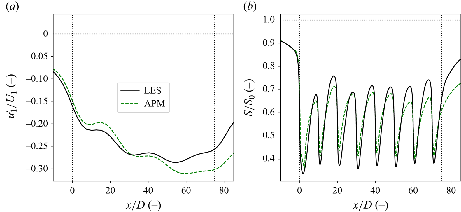
Finally, by comparing the velocity deficits in figure 10, one sees that the APM slightly underpredicts the velocity deficit in the first half of the farm and strongly overpredicts it in the second half and the farm wake. To see this more accurately, figure 11(a) shows the difference between the centreline velocity deficit for both the LES and APM results. At the farm entrance, the APM captures the blockage fairly well, although the predicted velocity is slightly too high. Halfway through the farm, the APM predicts that the velocity deficit increases drastically, resulting in a lower velocity than the LES. As a result, the APM overpredicts the farm wake as discussed above. The discrepancies in the velocity estimate are reflected in the turbine-level velocity, as shown in figure 11(b). This is consistent across most of the analysed cases, as shown in Appendix D, except for some H300 cases where the location of strong resonant lee waves does not match the LES.
Streamwise velocity deficits through the centre of the farm of the LES (solid, black) and APM output (dashed, green) for the case H500- $\Delta \theta$5-
 $\varGamma$4. (a) The mesoscale velocity deficit. (b) The average velocity across a tube with the turbine diameter. The dotted lines denote the wind farm region.

Overall, we conclude that the APM captures the relevant physics well, and produces realistic flow fields. It is worth noting that this good qualitative agreement between the APM and LES has been achieved with minimal tuning. The only parameters fitted in this work are those describing the wind-farm-induced turbulent momentum flux.
4.2.2. Power output
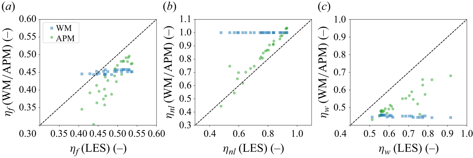
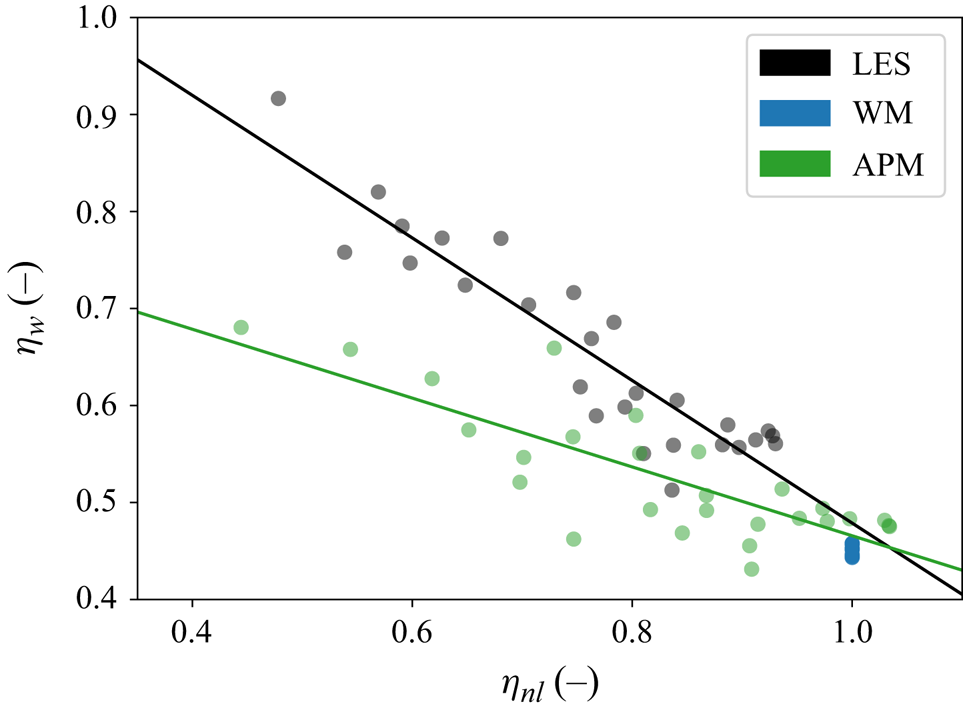
The aim of the APM is to provide the power predictions that include the effects of blockage and other mesoscale phenomena on wind farm performance. These are farm-wide effects, and are therefore best quantified using farm-wide metrics. We follow Allaerts & Meyers (Reference Allaerts and Meyers2018) by using the non-local wind farm efficiency  $\eta _{nl}$, which is the ratio of the average power output of the first-row turbines and an identical turbine operating on its own:
 \begin{equation} \eta_{nl} = \frac{P_1}{P_0}. \end{equation}
This  $P_0$ is the same power output that was used to scale the results in § 4.1.2. The non-local efficiency captures the decrease in power output caused by the upstream effects of the turbines operating in a farm. Within the studied dataset, there are large variations in
 $\eta _{nl}$, with values going from roughly 1 for cases with minimal blockage to as low as 0.55 for some cases. Additionally, following Allaerts & Meyers (Reference Allaerts and Meyers2018), we define
 \begin{equation} \eta_f=\eta_{nl}\eta_w,\quad \eta_w=\frac{P_{avg}}{P_1}, \end{equation}
where  $\eta _f$ is the total farm efficiency and
 $\eta _w$ is the wake efficiency, defined as the ratio between the average power output of all turbines
 $P_{avg}$ to that of the front-row average
 $P_1$. The farm efficiency is a measure the performance of a wind farm as a whole. The wake efficiency links the farm and non-local efficiencies, and represents the combined effects of the favourable pressure gradient across the farm and the turbine interactions within it. Additionally, it is the classical way that wake effects have been quantified in the past. Recent metrics that isolate the effect of turbine wake interactions may be of interest, but are not considered further here (Kirby et al. Reference Kirby, Nishino and Dunstan2022).
Figure 12 shows the farm, non-local and wake efficiencies of the studied wind farm for all cases, as obtained by LES, the uncoupled wake model and the APM. The uncoupled wake model performs quite poorly, and its outputs do not vary significantly between the different flow cases. This is to be expected, as the main difference between the flow cases are the stratification levels in the capping inversion and the free atmosphere, which the wake model does not take into account. As a result, the wake model cannot capture the large variations and trends in the different efficiencies. The slight variance in its predictions is due to small differences in the wind veer and shear, and turbulence intensity at hub height. Additionally, it does not model any upstream effects, so  $\eta _{nl}$ is always 1. This is offset by a consistent underestimation of the wake efficiency. While this results in a roughly correct average farm efficiency when averaging over all cases, it is clear that this is because the errors in
 $\eta _{nl}$ and
 $\eta _w$ cancel each other out.
Comparison of the farm (a), non-local (b) and wake (c) efficiencies as found by LES (horizontal axes) for all cases with those predicted by the APM (green circles) and the uncoupled wake model (blue squares).

In contrast, the APM captures the trends of both  $\eta _f$ and
 $\eta _{nl}$ quite well. This is expected after § 4.2.1, which found that the APM captures the general behaviour of the atmospheric flow, and § 4.1.2, which showed that the VM method can provide good estimates for the power output. Nevertheless, as discussed in § 4.2.1, the APM consistently slightly overestimates the velocity in the entrance region. This results in an overestimation of the non-local efficiency as well, leading to an offset between the APM and LES, and an average error of 7 %. This is better than that of the uncoupled wake model, which on average overestimates
 $\eta _{nl}$ by 24 %. For three of the H1000 cases, where blockage effects are very weak, the APM predicts a non-local efficiency above one, as its velocity deficit becomes smaller than that of the uncoupled wake model. In contrast, the wake efficiency is consistently underestimated, although the APM still significantly outperforms the uncoupled wake model. The discrepancies in
 $\eta _w$ are mainly due to the overestimation of
 $P_1$, the underestimation of the velocity in the second half of the farm and the issues with the VM method found in the previous section.
The relation between the unfavourable pressure gradient upstream of the farm and the favourable one throughout it, as reported by Lanzilao & Meyers (Reference Lanzilao and Meyers2024), results in a relation between  $\eta _{nl}$ and
 $\eta _w$ as well. Specifically, as
 $\eta _{nl}$ decreases due to higher blockage,
 $\eta _w$ increases, as shown in figure 13. Despite this balancing effect, blockage is still detrimental to the overall power output of the farm. Figure 13 also shows that the APM can reproduce these trends, although the slopes are not exactly the same.
Relation between  $\eta _{nl}$ and
 $\eta _w$, as found by LES (black), the APM (green) and the uncoupled wake model (blue). The lines represent least-squares fits.

In conclusion, the APM is able to predict the variation of wind farm performance across different flow cases. More importantly, it consistently and significantly outperforms the uncoupled wake model, which is the default approach taken by the wind energy community. Finally, we again want to emphasize that this has been achieved without any power-based tuning of the model parameters.
5. Conclusion
This work presents a new version of the APM first introduced by Allaerts & Meyers (Reference Allaerts and Meyers2019), and improves the mesoscale parametrization of large wind farms. This was mainly done in three ways. First, we added an explicit ad hoc parametrization of the increased momentum entrainment above a wind farm, which allows for general turbine layouts. Second, we presented a large-scale overhaul of the wake-model coupling. For this, a new method was developed based on ensuring that the velocity fields of the APM and the wake model were consistent with each other. Third, we found that dispersive stresses play an important role at the farm entrance, and significantly contribute to the global blockage effect. Using the wake-model coupling, these stresses can be easily incorporated into the APM.
The VM method was validated independently of the APM using a dataset of 27 LES simulations set up by Lanzilao & Meyers (Reference Lanzilao and Meyers2024). The matching of the mesoscale velocity fields resulted in a better approximation of the turbine-level velocity fields, and drastically improved the power predictions when compared with the uncoupled wake model. This good performance was consistent, with the coupled wake model outperforming its uncoupled counterpart for all analysed flow cases. Additionally, we identified the main sources of error as being the unidirectional approximation, and the accuracy of the wake models in representing the turbine wakes. The former could easily be addressed in future work, as the VM method is straightforward to extend to two-directional flow.
Additionally, we performed a momentum budget analysis on the LES results, and found that the dispersive stresses are important to mesoscale wind farm flows. At the farm entrance, their effect can be as strong as the peak pressure gradient, significantly contributing to the global blockage effect. Since the APM filter results in a similar resolution to numerical weather models, dispersive stresses are presumably also important to incorporate in wind farm parametrizations for those models, and we recommend this for future research.
Finally, the improved APM was validated using the same LES data. The APM performs well, as it captures most of the relevant mesoscale flow phenomena, especially when it comes to stratification effects. There is good qualitative agreement between the LES and the APM for the appearance of gravity waves, and the associated blockage, farm pressure gradients, resonant lee waves and flow speed-up around the sides of the farm. However, the reduced-order nature of the APM prevents it from capturing the IBL growth, and changes in the ABL vertical structure. Moreover, the APM slightly overestimates the velocity in the first half of the farm, and underestimates it in the second half. Despite this mismatch, the good qualitative match allows the APM to model the effect of atmospheric stratification on turbine power output. For all analysed metrics, the APM significantly outperforms a standard engineering wake model. Regarding the effect of blockage on the front-row turbines, the APM overestimates the wind farm's non-local efficiency, but reproduces very well the variation in this efficiency across all cases. This allows it to find the same relation between the non-local and the wake and farm efficiencies as the LES. Given the good performance of the underlying VM method, we expect any further improvement to the APM to translate directly into more accurate power predictions. Additionally, this was achieved without any power-based tuning. This makes the APM a promising tool for studying the next generation of offshore wind farms.
Currently, the APM can still only simulate wind farms in highly idealized conditions. In reality, the simple CNBL profiles used in this study are complicated by various phenomena, such as ABL stability effects or mesoscale systems already present in the atmosphere. Moreover, both atmospheric conditions and wind farm operational settings are rarely steady state, with transient effects being important for control problems. Finally, the current turbulence parametrization does not include the effects of background turbulence intensity, and could be improved by an explicit modelling of turbulent transport phenomena. Future work should extend the APM to include these flow features. The model should also be further compared with experimental and operational data.
Acknowledgements
The computational resources and services used in this work were provided by the VSC (Flemish Supercomputer Center), funded by the Research Foundation Flanders (FWO) and the Flemish Government department EWI.
Funding
This research has been supported by the Energy Transition Fund of the Belgian Federal Public Service for Economy, SMEs, and Energy (FOD Economie, KMO, Middenstand en Energie), and by the European Union Horizon Europe Framework programme (HORIZON-CL5-2021-D3-03-04) under grant agreement no. 101084205.
Declaration of interests
The authors report no conflict of interest.
Data availability statement
An open-source version of the code implementing the APM, including the developments in this work, can be found at https://doi.org/10.48804/XMNVVY.
Author contributions
K.D. and J.M. jointly re-derived the model, and incorporated the additional linear terms, dispersive stresses and the increased momentum flux into the APM. K.D., L.L. and J.M. jointly developed the VM coupling method. K.D. and J.M. jointly set up the validation studies. K.D. and L.L. performed code implementations and carried out the simulations. K.D., L.L. and J.M. jointly wrote the manuscript.
Appendix A. Detailed derivation of the lower-layer continuity equation
This appendix derives the continuity equation for the lower layer of the APM. We start by applying the filtering and height-averaging operations (2.1) and (2.5) to the Reynolds-averaged, steady-state continuity equation. The former of these can simply be brought into the divergence operator, which results in
 \begin{equation} \langle\boldsymbol{\nabla}\boldsymbol{\cdot}\bar{\boldsymbol{u}}\rangle_1=0. \end{equation}
To obtain derivatives with respect to the height-averaged velocities, the integration of the height-averaging operator is brought into the divergence operator, by changing the order of operation using Leibniz's differentiation rules (Allaerts & Meyers Reference Allaerts and Meyers2019). This gives
 \begin{align} \langle\boldsymbol{\nabla}\boldsymbol{\cdot}\bar{\boldsymbol{u}}\rangle_1 &= \frac{1}{z_1}\left[\boldsymbol{\nabla}_h\boldsymbol{\cdot}\int_0^{z_1}\bar{\boldsymbol{u}}_h\,\mathrm{d}z- \bar{\boldsymbol{u}}_h\vert_{z_1}\boldsymbol{\cdot}\boldsymbol{\nabla}_h z_1\right]+\frac{1}{z_1}\left(\int_0^{z_1} \frac{\partial\bar{w}}{\partial z}\mathrm{d}z\right) \nonumber\\ &= \frac{1}{z_1}\left[\boldsymbol{\nabla}_h\boldsymbol{\cdot}\int_0^{z_1}\bar{\boldsymbol{u}}_h\,\mathrm{d}z- \bar{\boldsymbol{u}}_h\vert_{z_1}\boldsymbol{\cdot}\boldsymbol{\nabla}_h z_1\right]+\frac{1}{z_1}\bar{w}\vert_{z_1}. \end{align}
By then applying the definition of the pliant surface  $z_1$ (2.3), we find the lower-layer continuity equation for the APM (Allaerts & Meyers Reference Allaerts and Meyers2019). For upper-layer continuity and the momentum equations, the procedure is analogous, and results in (2.8)–(2.10).
Appendix B. Wind-farm-induced momentum flux tuning
We fit the coefficients  $a_{\tau }$ and
 $d_{\tau }$ to the 27 LES cases from Lanzilao & Meyers (Reference Lanzilao and Meyers2024) used throughout this paper and summarized in tables 1 and 2. From this dataset, we have constructed LES-based APM states, as described in § 2.4. This way,
 $\langle \bar {\boldsymbol {u}}\rangle _1$ and
 $\langle \bar {\boldsymbol {u}}\rangle _2$ are known for all cases. Based on the associated precursor simulations, we compute
 $D$. We then apply the Gaussian filter described in (2.2) to the vertical momentum fluxes, and evaluate
 $\bar {\tau }_{03}$ at
 $z_1$ for all cases. This gives us data for the first two terms in (2.21), allowing us to calculate
 $\Delta \boldsymbol {\tau }_{{wf}}$ directly from the LES. We average the resulting fields along the spanwise direction within the wind farm boundaries, and fit the coefficients along the streamwise direction. Figure 14 shows the LES profiles and the resulting fit for
 $\Delta \bar {\boldsymbol {\tau }}_{{wf}}$, Gaussian-filtered onto the APM grid.
Added wind farm momentum flux  $\Delta \bar {\boldsymbol {\tau }}_{{wf}}$ as calculated based on the LES data of Lanzilao & Meyers (Reference Lanzilao and Meyers2024). The line colours denote the boundary layer height. The fitted profile is indicated by the black line. The dotted lines indicate the wind farm region.

Appendix C. Solving procedure for the VM equation
This appendix discusses how the VM equation is solved.
Equation (3.12) is solved with a variational approach. Since  $\langle \bar {u}\rangle _{1}$ is known at the APM gridpoints, we use a collocation method, so that the test functions are Dirac-delta functions at the APM gridpoints inside
 $\varOmega _{{wf}}$.
To discretize  $u_b$, we write it as a finite sum of shape functions:
 \begin{equation} u_b=\sum_{i,j=1}^{N^s_x,N^s_j}u_{i,j}\phi_{i,j}(x,y), \end{equation}
where  $N^s_x$ and
 $N^s_j$ are the number of shape functions in the
 $x$ and
 $y$ directions, respectively,
 $u_{i,j}$ are a set of coefficients and
 $\phi _{i,j}(x,y)$ are generic first-order shape functions with compact support:
 \begin{equation} \phi_{i,j}(x,y) = \max{\left(0,\left(1-\frac{\vert\vert x-x_i \vert\vert}{\Delta x_s}\right) \left(1-\frac{\vert\vert y-y_j \vert\vert}{\Delta x_s}\right)\right)}. \end{equation}
The shape function centres  $(x_i,y_j)$ are evenly spaced within
 $\varOmega _{{wf}}$, so that
 \begin{equation} x_i=x_{i-1}+\Delta x_s,\quad y_j=y_{j-1}+\Delta x_s, \end{equation}
where  $\Delta x_s$ is the spacing between the shape function centres. This spacing is determined by the parameter
 $\alpha$, so that
 \begin{equation} \alpha = \ell/\Delta x_s. \end{equation}
Choosing  $0<\alpha <\ell /\Delta x$, with
 $\Delta x$ the APM grid spacing, results in a least-squares formulation.
The choice of  $\alpha$ has a large effect on the performance of the VM method. If
 $\alpha$ is too low, the discretized
 $u_b$ does not have enough degrees of freedom to adequately reproduce the variations in
 $\langle \bar {u}\rangle _{1}$. However, a high value of
 $\alpha$ can lead to oscillations in
 $u_b$ on scales below the filter length that do not correspond to variations in
 $\langle \bar {u}\rangle _{1}$. By investigating the error on the reproduced
 $\langle \bar {u}\rangle _{1}$ for a range of
 $\alpha$ for the case H500-
 $\Delta \theta$5-
 $\varGamma$4, we find that
 $\alpha =0.8$ results in good performance.
Each APM gridpoint  $(x_t,y_t)$ then tests for the matching condition:
 \begin{equation} b_t = \sum_{i,j=1}^{N^s_x,N^s_j}A_{i,j,t}u_{i,j}, \end{equation}
where  $b_t$ is the right-hand side of (3.12) evaluated at
 $(x_t,y_t)$ and
 $A_{i,j,t}$ is given by
 \begin{align} A_{i,j,t} = \frac{1}{z_1}\int_{0}^{z_1}{\iint_{\varOmega_{{wf}}} G_\ell(x_t-x^{\prime},y_t-y^{\prime})\phi_{i,j}(x^{\prime},y^{\prime})f(z) \prod_{k=1}^{N_t}[1-W_k(x^{\prime},y^{\prime},z)]\,\mathrm{d}\kern0.06em x^{\prime}\,\mathrm{d}y^{\prime}\,\mathrm{d}z}. \end{align}
Whether the Gaussian filter or the height-averaging operation is applied first in (3.12) changes the resulting mesoscale velocity by less than  $0.01U_1$. In solving the equation, the height-averaging operator is applied first, as this is faster to compute. The integrals are all computed numerically using numpy and scipy routines, sped-up with the numba package (Lam, Pitrou & Seibert Reference Lam, Pitrou and Seibert2015).
Appendix D. Velocity comparisons for all analysed cases
Figure 15 shows the velocity deficits along the centreline of the farm for all analysed flow cases. The APM consistently over- and underpredicts the velocity in the first and second half of the farm, respectively, but otherwise captures the stratification effects quite well. The largest errors occur for the cases with low, strong capping inversions and weak atmospheric stratification above.
Lower-layer velocity perturbations through the centre of the farm of the LES (solid, black) and APM output (dashed, green) for all analysed cases. The dotted lines denote the wind farm region.