
1. Introduction
Ring structures arise in a diverse set of physical systems. In fluid mechanics, rings composed of multiple vortices are of particular interest and have been observed over a broad range of scales, from baths of superfluid helium (Yarmchuk, Gordon & Packard Reference Yarmchuk, Gordon and Packard1979) to hurricane eyewalls (Kossin & Schubert Reference Kossin and Schubert2004). Several theoretical studies have characterized the stability of polygonal vortex arrays composed of both point vortices (Thomson Reference Thomson1883; Havelock Reference Havelock1931; Aref et al. Reference Aref, Newton, Stremler, Tokieda and Vainchtein2003; Celli, Lacomba & Pérez-Chavela Reference Celli, Lacomba and Pérez-Chavela2011) and generalized vortices of finite area (Crowdy Reference Crowdy1999; Crowdy & Cloke Reference Crowdy and Cloke2002; Crowdy Reference Crowdy2003; Krishnamurthy et al. Reference Krishnamurthy, Wheeler, Crowdy and Constantin2019). Vortex arrays have also been observed in magnetized non-neutral plasmas (Schecter et al. Reference Schecter, Dubin, Fine and Driscoll1999; Durkin & Fajans Reference Durkin and Fajans2000) and in both bosonic and fermionic systems, where vortices play a critical role in superconductivity (Saarikoski et al. Reference Saarikoski, Reimann, Harju and Manninen2010). Ring structures may also form when particles are confined to an air–liquid interface. Magnetized spinning disks floating on a fluid bath are found to self-assemble into a variety of ordered structures including rings (Grzybowski, Stone & Whitesides Reference Grzybowski, Stone and Whitesides2000). Electrons levitated above a bath of superfluid helium may form ring structures, known as Wigner molecules, whose dynamics is influenced by the coupling of the electrons to an underlying capillary wavefield (Rousseau et al. Reference Rousseau, Ponarin, Hristakos, Avenel, Varoquaux and Mukharsky2009). We here investigate the rich set of dynamical behaviours that arise in rings composed of millimetric droplets that bounce on the surface of a vibrating liquid bath and interact through their common wavefield.
The surface of a fluid bath, vibrated vertically with frequency f and acceleration  $\gamma \sin ({2{\rm \pi} f t})$, will destabilize into a field of subharmonic standing Faraday waves for
 $\gamma >\gamma _F$, the Faraday threshold (Benjamin & Ursell Reference Benjamin and Ursell1954; Miles & Henderson Reference Miles and Henderson1990). The resulting Faraday wavefield oscillates with period
 $T_F=2/f$ and has a wavelength
 $\lambda _F$ that can be approximated using the water-wave dispersion relation. Above the bouncing threshold but below the Faraday threshold,
 $\gamma _B<\gamma <\gamma _F$, a millimetric fluid droplet may bounce indefinitely on the vibrating bath (Walker Reference Walker1978). Coalescence is prevented by a thin air layer between the droplet and the bath that is sustained during the drop's impact (Couder et al. Reference Couder, Fort, Gautier and Boudaoud2005a). The dependence of the drop's bouncing mode on the droplet radius
 $R$, vibrational frequency
 $f$ and vibrational acceleration
 $\gamma$ has been studied in detail (Protière, Boudaoud & Couder Reference Protière, Boudaoud and Couder2006; Eddi et al. Reference Eddi, Terwagne, Fort and Couder2008; Moláček & Bush Reference Moláček and Bush2013a,b; Wind-Willassen et al. Reference Wind-Willassen, Moláček, Harris and Bush2013; Galeano-Rios, Milewski & Vanden-Broeck Reference Galeano-Rios, Milewski and Vanden-Broeck2017). As
 $\gamma$ is increased progressively beyond
 $\gamma _B$, the droplet undergoes a period-doubling transition and eventually becomes resonant with the Faraday wave period,
 $T_F$, leading to a significant increase in the wave energy. For
 $\gamma >\gamma _W$, the walking threshold, the resonant droplet destabilizes into steady, rectilinear motion across the surface of the bath, propelled by the waves generated at its previous impacts (Couder et al. Reference Couder, Protiere, Fort and Boudaoud2005b; Protière et al. Reference Protière, Boudaoud and Couder2006). The closer
 $\gamma$ is to
 $\gamma _F$, the longer the surface waves persist, and the more strongly the drop's motion is influenced by its past (Eddi et al. Reference Eddi, Sultan, Moukhtar, Fort, Rossi and Couder2011b). Remarkably, in the high-memory limit
 $\gamma \rightarrow \gamma _F$, walking droplets have exhibited a variety of quantum-like features, as reviewed elsewhere (Bush Reference Bush2015; Bush et al. Reference Bush, Couder, Gilet, Milewski and Nachbin2018). Notably, this hydrodynamic pilot-wave system is similar in form to the double-solution pilot-wave theory of quantum dynamics proposed by Louis de Broglie, who envisaged microscopic particles moving in resonance with a guiding wavefield (de Broglie Reference de Broglie1956; Colin, Durt & Willox Reference Colin, Durt and Willox2017).
Multiple bouncing droplets may interact at a distance through their common wavefield. Depending on the distance between the drops, this interaction can be attractive or repulsive. Pairs of drops can form bound states with a discrete set of inter-drop distances and exhibit a variety of dynamical behaviours including orbital (Couder et al. Reference Couder, Protiere, Fort and Boudaoud2005b; Protière et al. Reference Protière, Boudaoud and Couder2006; Protière, Bohn & Couder Reference Protière, Bohn and Couder2008; Oza et al. Reference Oza, Siéfert, Harris, Moláček and Bush2017), promenading (Borghesi et al. Reference Borghesi, Moukhtar, Labousse, Eddi, Fort and Couder2014; Arbelaiz, Oza & Bush Reference Arbelaiz, Oza and Bush2018), oscillatory (Couchman, Turton & Bush Reference Couchman, Turton and Bush2019) and ratcheting (Eddi et al. Reference Eddi, Terwagne, Fort and Couder2008; Galeano-Rios et al. Reference Galeano-Rios, Couchman, Caldairou and Bush2018) motions. When more than two drops interact, they can self-organize into periodic lattices (Protière et al. Reference Protière, Couder, Fort and Boudaoud2005; Eddi et al. Reference Eddi, Decelle, Fort and Couder2009). These lattices can go unstable to collective motion, such as lateral vibrations (Eddi, Boudaoud & Couder Reference Eddi, Boudaoud and Couder2011a), drifting (Eddi et al. Reference Eddi, Terwagne, Fort and Couder2008) or bulk rotation (Lieber et al. Reference Lieber, Hendershott, Pattanaporkratana and Maclennan2007). The dynamics of multi-droplet systems constrained by submerged topography has also been considered. When droplets are confined to a two-dimensional lattice of submerged circular wells, spin–spin correlations may emerge (Sáenz et al. Reference Sáenz, Pucci, Goujon, Cristea-Platon, Dunkel and Bush2018). Strings of walking droplets confined by a submerged annular channel form a coherent wavefield that allows them to walk faster than an individual droplet (Filoux, Hubert & Vandewalle Reference Filoux, Hubert and Vandewalle2015). A droplet chain that spans the entire circumference of an annular channel is found to destabilize through either out-of-phase oscillations or propagating solitary-like waves as the vibrational acceleration is increased (Thomson, Couchman & Bush Reference Thomson, Couchman and Bush2020a; Thomson, Durey & Rosales Reference Thomson, Durey and Rosales2020b), phenomena similar to those predicted by theoretical studies of one-dimensional driven dissipative lattices (Ebeling et al. Reference Ebeling, Erdmann, Dunkel and Jenssen2000). By studying rings without the radial constraint imposed by the submerged channel, we here uncover an even richer variety of dynamical behaviours.
A variety of theoretical models have been developed to describe the dynamics of walking droplets in various settings (see review of Turton, Couchman & Bush Reference Turton, Couchman and Bush2018). We here follow the path initiated by Moláček & Bush (Reference Moláček and Bush2013a,Reference Moláček and Bushb), who developed coupled equations for a drop's vertical and horizontal motion from a suitable reduction of the Navier–Stokes equations. In order to describe resonant drops, specifically those in a period-doubled bouncing mode, Oza, Rosales & Bush (Reference Oza, Rosales and Bush2013) time-averaged the equations of Moláček & Bush (Reference Moláček and Bush2013b) over a bouncing period,  $T_F$, to obtain a stroboscopic trajectory equation governing the drop's horizontal motion. The stroboscopic model implicitly assumes that the drop's periodic vertical motion is unchanging and a fitting parameter is used to prescribe the phase at which the droplet impacts the bath. While this assumption of a constant impact phase was satisfactory when modelling the dynamics of single droplets, it was found to be inadequate in modelling the stability of orbiting (Oza et al. Reference Oza, Siéfert, Harris, Moláček and Bush2017) and promenading (Arbelaiz et al. Reference Arbelaiz, Oza and Bush2018) pairs, where variations in the impact phase induced by wave-mediated interactions with neighbouring droplets were significant. Informed by high-speed imaging of a drop's vertical motion across a range of parameters, Couchman et al. (Reference Couchman, Turton and Bush2019) developed a model that accounts for the dependence of a drop's impact phase on the bath's vibrational acceleration, the local wave amplitude beneath a drop and the droplet radius. Their study demonstrated that accounting for modulations in the impact phase was essential for rationalizing the observed stability of droplet pairs. Such phase variations are expected to be similarly important when considering the stability and dynamics of larger multi-drop systems; hence, their variable-phase stroboscopic model will be adopted in what follows.
In § 2, we characterize experimentally the discrete set of rings that can be constructed from a given number of drops. We then characterize how each ring destabilizes when the bath's vibrational acceleration is increased progressively. In § 3, we present both linear stability analysis and numerical simulations based on the theoretical model of Couchman et al. (Reference Couchman, Turton and Bush2019). Our theoretical developments provide rationale for much of the observed behaviour, including the set of stable rings, their various instabilities, and the subsequent dynamics arising as the vibrational acceleration is increased. In § 4, we discuss extensions of our work to more complex droplet lattices and aggregates, and draw comparisons with the stability of ring structures found in other areas of physics.
2. Experiments
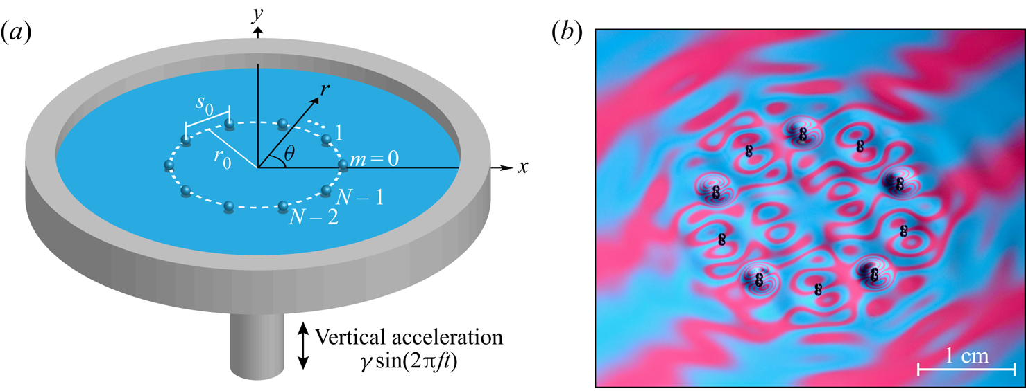
A schematic of our experimental set-up is illustrated in figure 1(a). A bath of silicon oil (density  $\rho = 949\ \textrm {kg}\,\textrm {m}^{-3}$, surface tension
 $\sigma = 20.6\times 10^{-3}\ \textrm {N}\,\textrm {m}^{-1}$, kinematic viscosity
 $\nu = 20\ \textrm {cSt}$,
 $\text {depth} =7\ \textrm {mm}$) is shaken in the vertical direction with frequency
 $f=80\ \textrm {Hz}$ and acceleration
 $\gamma \sin (2 {\rm \pi}f t)$. The Faraday threshold is
 $\gamma _F \approx 4.25 g$, where
 $g$ denotes the gravitational acceleration. The associated Faraday wavelength, as may be approximated from the water-wave dispersion relation, is
 $\lambda _F = 4.75$ mm. A detailed description of the shaker apparatus is provided by Harris & Bush (Reference Harris and Bush2015). Droplets of a desired size, composed of the same silicon oil, are generated using a piezoelectric droplet generator (Harris, Liu & Bush Reference Harris, Liu and Bush2015). An overhead camera is used to record the drops’ horizontal motion and a high-speed camera is used to record a side view of the vertical motion. Following the notation of Moláček & Bush (Reference Moláček and Bush2013a), we use
 $(i,j)^k$ to denote a bouncing mode in which the drop's vertical motion has a period of
 $i$ times that of the bath vibration,
 $T_F/2$, and impacts the bath
 $j$ times during this period. For the same mode
 $(i,j)$, it is sometimes possible for a drop to bounce with either a relatively low or high amplitude, as distinguished by
 $k=\{ 1,2\}$, respectively. During our experiments, a transparent lid covers the bath in order to minimize the influence of ambient air currents.
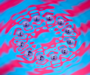
(a) A schematic of the experimental set-up (not to scale). A ring composed of  $N$ drops, of radius
 $r_0$ and corresponding side length
 $s_0$, bounces on a vertically vibrating liquid bath. The bath radius,
 $8$ cm, is 4 times larger than the largest ring radius considered,
 $r_0 \approx 2\ \textrm {cm}$, to ensure that the rings do not interact with the bath's boundary. (b) A snapshot of a ring of
 $N=10$ drops with radius
 $r_0 = 9.50$ mm. Here, each drop bounces out-of-phase relative to its neighbours, as evident in the alternating structure of the wavefield surrounding each drop. The wavefield is visualized by illuminating the bath with a striped pattern of coloured light (Harris et al. Reference Harris, Quintela, Prost, Brun and Bush2017).

We construct rings from individual drops of radius  $R=0.36 \pm 0.01\ \textrm {mm}$. At the vibrational accelerations considered in our experiments, the drops bounce in the resonant
 $(2,1)$ bouncing mode; thus, they may bounce either in synchrony (in-phase) or with a phase shift of
 ${\rm \pi}$ (out-of-phase) relative to each other. Each ring is characterized by its drop number
 $N$, radius
 $r_0$, and the relative bouncing phase of neighbouring drops, either in-phase (
 $\zeta =1$) or out-of-phase (
 $\zeta = -1$). An example of a ring with
 $N=10$,
 $r_0/\lambda _F=2.00$ and
 $\zeta =-1$ is shown in figure 1(b). To construct a ring, we first set the bath's vibrational acceleration to
 $\gamma = 0.7 \gamma _F$, which is below the walking threshold of an individual drop,
 $\gamma _W = 0.75 \gamma _F$. Each drop bounces in place in the
 $(2,1)$ mode, as is consistent with the regime diagram of Wind-Willassen et al. (Reference Wind-Willassen, Moláček, Harris and Bush2013) for individual drops. A partially submerged needle, which creates a droplet-repelling meniscus in its vicinity, is then used to arrange the drops into a ring of the desired size. To facilitate the construction of larger, more fragile rings, it was helpful to partially submerge into the bath a vertical rod, whose meniscus acts to repel nearby drops. Two needles were then used to wrap a chain of drops around the rod. Once the ring was formed, the rod could be removed from its centre. Note that when neighbouring drops are bouncing out of phase,
 $\zeta = -1$, a periodic ring can only be achieved if
 $N$ is even.
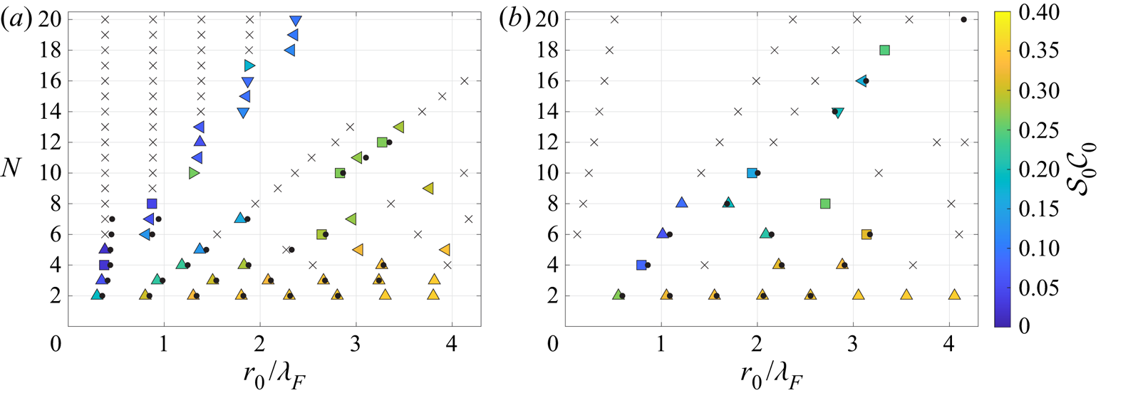
For a given drop number  $N$ and relative bouncing phase
 $\zeta$, rings could only be constructed with a discrete set of possible radii
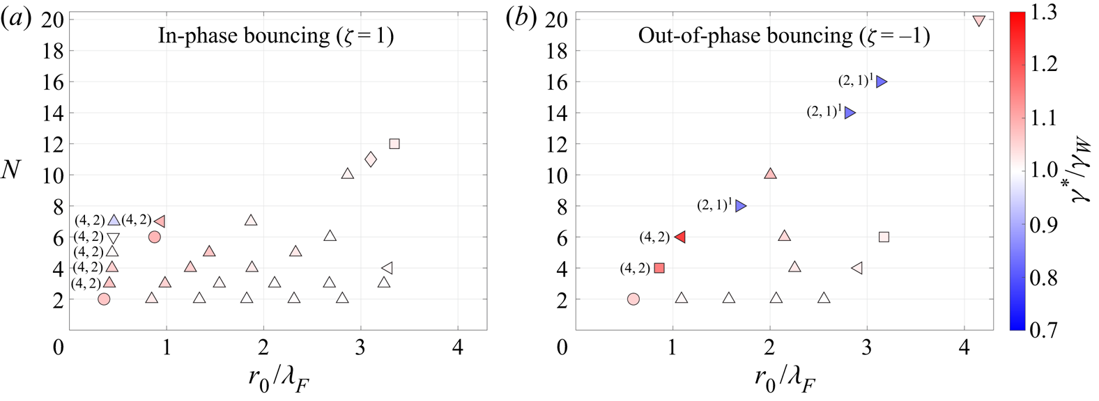
 $r_0$, as shown in figure 2. Rings created with intermediate radii were unstable and collapsed into a variety of shapes. For instance, while a ring of
 $N=8$,
 $r_0/\lambda _F \approx 2$ and
 $\zeta = 1$ could be built around a central rod, the drops were found to spontaneously rearrange into a square following the rod's removal. The possible values of
 $r_0$ are highly dependent on both
 $N$ and
 $\zeta$. For example, with
 $\zeta = 1$ we could not construct
 $N=8$ or
 $N=9$ rings, while
 $N=7$ and
 $N=10$ rings were viable. For
 $\zeta =-1$, an
 $N=8$ ring is possible. For both
 $\zeta = \pm 1$, the number of possible radii
 $r_0$ generally decreases as
 $N$ increases. It was difficult to construct rings with
 $r_0/\lambda _F \gtrsim 3$ due to the weak interactions between neighbouring drops at such large ring radii. Note that the data in figure 2 for
 $N=2$ correspond to those reported for droplet pairs by Couchman et al. (Reference Couchman, Turton and Bush2019).
Rings that could be constructed experimentally, as characterized by their drop number  $N$ and non-dimensional radius
 $r_0/\lambda _F$ for drops bouncing (a) in-phase (
 $\zeta =1$) and (b) out-of-phase (
 $\zeta =-1$) relative to their nearest neighbours. The marker colour denotes the vibrational acceleration,
 $\gamma ^*$, normalized by the walking threshold of a single free drop,
 $\gamma _W = 0.75 \gamma _F$, at which the ring destabilized into some form of horizontal motion. The marker shape denotes the type of instability observed: in-phase radial oscillations (
 ), out-of-phase radial oscillations (
 ), out-of-phase azimuthal oscillations (
 ), azimuthal travelling waves (
 ), orbital motion (
 ), irregular rearrangements (
 ) and more complex, unclassified motions (
 ). All drops were observed to be in the
 $(2,1)^2$ bouncing mode in the vicinity of
 $\gamma ^*$, except for the special cases noted as being in
 $(2,1)^1$ or
 $(4,2)$ modes.
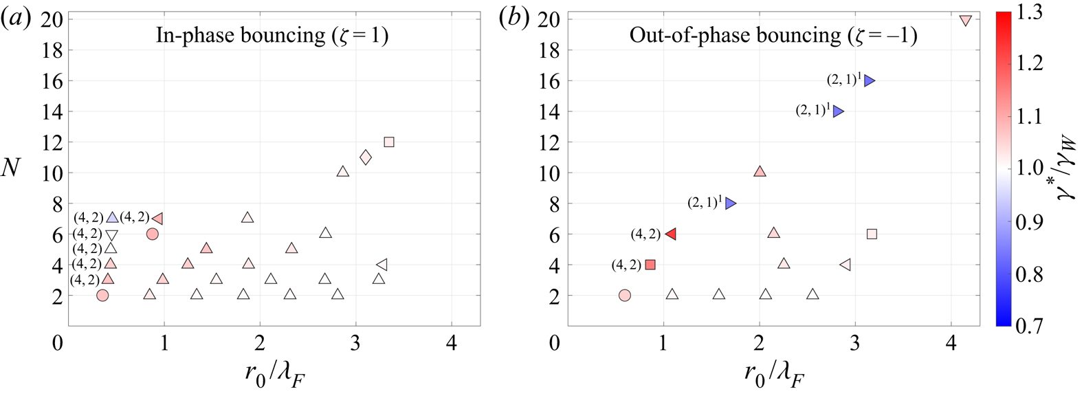
Once a ring had been constructed, we slowly increased  $\gamma$ until the ring destabilized in some fashion. This instability threshold, denoted by
 $\gamma ^*$, is indicated by the colour of the markers in figure 2. The bouncing mode of each ring was also determined at the instability threshold
 $\gamma ^*$ using a high-speed camera. The majority of rings were found to be in the
 $(2,1)^2$ mode at
 $\gamma ^*$ and to destabilize above the walking threshold of a single drop,
 $\gamma ^*>\gamma _W$. For a given
 $N$, we observed that rings with small
 $r_0$ are generally the most stable and that
 $\gamma ^*$ progressively decreases as
 $r_0$ increases, approaching
 $\gamma _W$ at the largest
 $r_0$ considered. There were two notable exceptions to this trend, occurring when the rings were composed of drops in a different bouncing mode. First, three
 $\zeta = -1$ rings with
 $(N, r_0/\lambda _F)= (8, 1.68)$,
 $(14, 2.81)$ and
 $(16, 3.13)$ destabilized well below
 $\gamma _W$, at the
 $(2,1)^1$ to
 $(2,1)^2$ bouncing mode transition, as denoted by the right-facing triangles (
 ) in figure 2(b). Second, the three
 $\zeta = 1$ rings with
 $N=5$,
 $6$,
 $7$ and
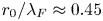 $r_0/\lambda _F\approx 0.45$, bouncing in the
 $(4,2)$ mode at
 $\gamma ^*$, destabilized close to or below
 $\gamma _W$.
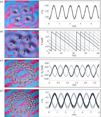
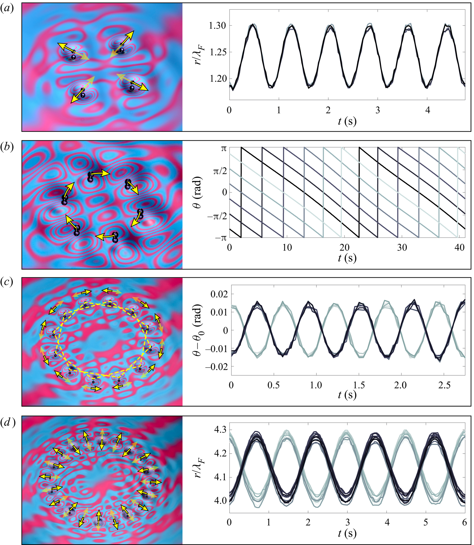
The shape of each marker in figure 2 denotes the type of instability observed at  $\gamma ^*$. The most common type of instability was in-phase radial oscillations (
 ), as shown in figure 3(a). In two cases,
 $(N, r_0/\lambda _F, \zeta ) = (6, 0.45, 1)$ and
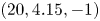 $(20, 4.15, -1)$, out-of-phase radial oscillations (
 ) were observed, as shown in figure 3(d), characterized by a phase difference of
 ${\rm \pi}$ between the radial oscillations of neighbouring drops. Instabilities in the azimuthal direction also arose, including purely orbital motion (
 , see figure 3b) and out-of-phase azimuthal oscillations (
 , see figure 3c). Notably, the motion of the
 $N=12$,
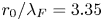 $r_0/\lambda _F=3.35$,
 $\zeta =1$ ring in figure 3(c) corresponds to the out-of-phase, rigid-body rotations of two hexagonal sub-lattices. Videos of the instabilities shown in figure 3 are presented in supplementary movie 1 available at https://doi.org/10.1017/jfm.2020.648. The ring of
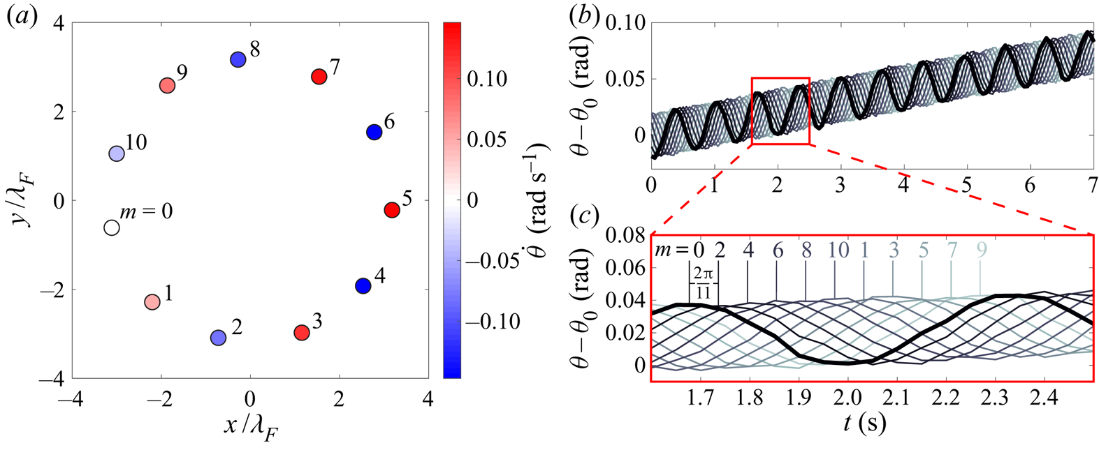
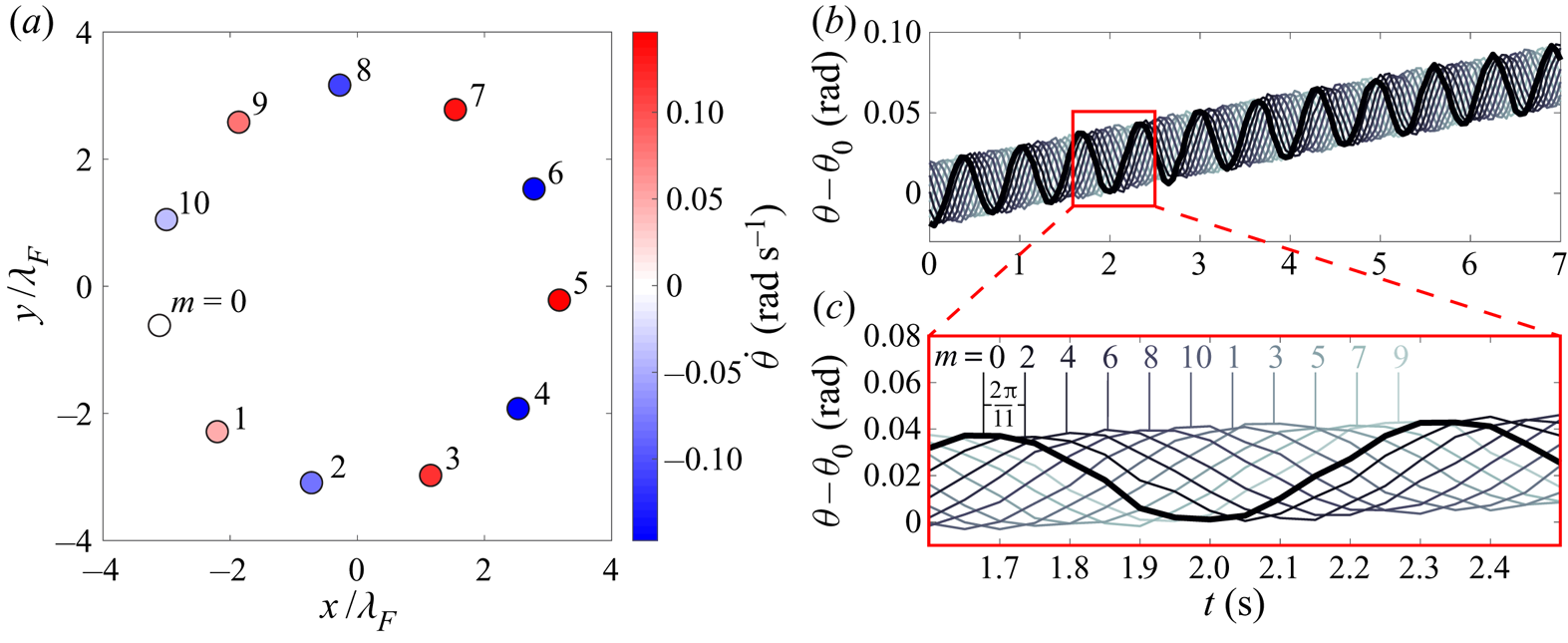
 $N=11$,
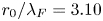 $r_0/\lambda _F=3.10$,
 $\zeta =1$ also destabilized into azimuthal oscillations. However, the geometric frustration caused by the odd
 $N$ results in a travelling wave in the azimuthal direction (
 ), as shown in figure 4 and supplementary movie 2. Note that in figure 4, the angular oscillation of every second drop has a phase difference of
 $2{\rm \pi} / 11$, and a slow net rotation of the entire ring is evident.
Examples of instabilities observed at the instability threshold,  $\gamma ^*$. In each panel (a–d), a snapshot of the ring is shown on the left, with arrows illustrating the drops’ horizontal motion. An accompanying time series of each drop's radial,
 $r(t)$, or azimuthal,
 $\theta (t)$, coordinate is shown on the right. (a) In-phase radial oscillations for a ring of
 $N=4$,
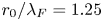 $r_0/\lambda _F = 1.25$ and
 $\zeta = 1$. (b) Orbital motion for a ring of
 $N=6$,
 $r_0/\lambda _F = 0.876$ and
 $\zeta = 1$. (c) Out-of-phase azimuthal oscillations for a ring of
 $N=12$,
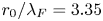 $r_0/\lambda _F = 3.35$ and
 $\zeta = 1$. The time series reflect angular displacements about each drop's equilibrium angle
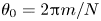 $\theta _0=2{\rm \pi} m/N$. (d) Out-of-phase radial oscillations for a ring of
 $N=20$,
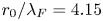 $r_0/\lambda _F = 4.15$ and
 $\zeta = -1$. See supplementary movie 1.
The travelling, azimuthal wave observed at the instability threshold  $\gamma ^*$ for a ring of
 $N=11$,
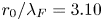 $r_0/\lambda _F=3.10$ and
 $\zeta =1$. (a) A snapshot of the ring at time
 $t=2$ seconds showing the instantaneous angular speed of each drop. (b) The angular displacement of each drop from its initial equilibrium position,
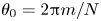 $\theta _0 = 2 {\rm \pi}m /N$, as a function of time,
 $t$. The curve corresponding to drop
 $m=0$ is highlighted in black for reference. (c) A close-up view of the red box in (b) illustrates that the angular oscillation of each drop has a phase shift of
 $2{\rm \pi} /11$ relative to its second-nearest neighbour. See supplementary movie 2.
In some cases, more exotic instabilities were observed. For example, the three rings that destabilized at the  $(2,1)^1$ to
 $(2,1)^2$ bouncing mode transition (denoted by dark blue
 markers in figure 2b), spontaneously rearranged into new, typically amorphous structures that then remained stable, instabilities that we refer to as irregular rearrangements. An example of such a rearrangement is shown in supplementary movie 3a for the ring
 $N=14$,
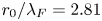 $r_0/\lambda _F = 2.81$,
 $\zeta = -1$. More complex radial or azimuthal motions were also observed, as indicated by (
 ) markers in figure 2. For instance, in the
 $N=7$,
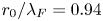 $r_0/\lambda _F=0.94$,
 $\zeta = 1$ ring shown in supplementary movie 3b, the drops tended to oscillate radially out-of-phase with their neighbours, but the geometric frustration caused by the odd
 $N$ complicated the motion.
We also briefly investigated how the dynamics of rings evolved as  $\gamma$ was increased progressively beyond
 $\gamma ^*$. The
 $N=6$,
 $r_0/\lambda _F=0.876$,
 $\zeta = 1$ ring, which initially went unstable to orbital motion at
 $\gamma ^* = 1.09\gamma _W$, developed a radial instability for
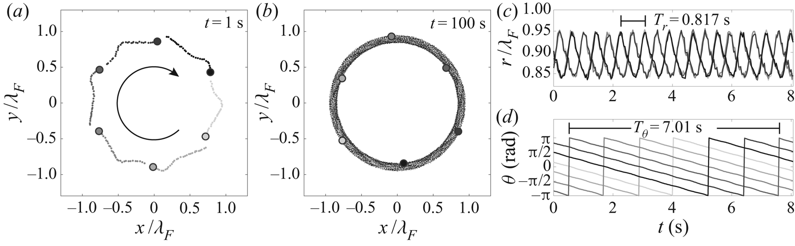
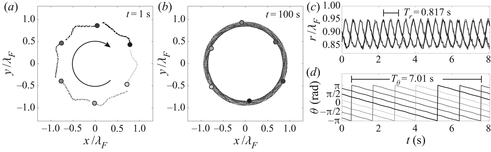
 $\gamma >\gamma ^*$, leading to the coupled radial and angular motion shown in figure 5 and supplementary movie 4. In this case, the ratio of the orbital and radial period is irrational,
 $T_\theta / T_r \approx 8.58\ldots\,$, leading to quasi-periodic motion. In most cases, the kinetic energy of the drops was observed to increase progressively with
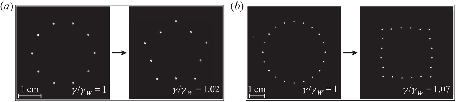
 $\gamma$ until a critical value was reached at which the ring broke apart. However, in two cases, the rings were observed instead to self-assemble into pentagonal and square structures, as shown in figure 6 and supplementary movie 5. These polygonal structures are stable following the rearrangement, but eventually collapse at higher
 $\gamma$ into a denser array.
The quasi-periodic wobbling orbital motion exhibited by a ring of  $N=6$,
 $r_0/\lambda _F=0.876$ and
 $\zeta = 1$ at
 $\gamma /\gamma _W = 1.20 > \gamma ^*/\gamma _W = 1.09$: (a and b) show the trajectories of each drop after
 $t=1$ s and
 $t=100$ s, respectively; (c and d) show the radial,
 $r(t)$, and azimuthal,
 $\theta (t)$, coordinates of each drop, respectively. Note that the ratio of the periods of the angular and radial motion
 $T_\theta / T_r \approx 8.58\ldots$ is irrational, leading to the dense packing of an annular region in the
 $xy$-plane over time, as evident in (b). See supplementary movie 4.
(a) Drops in a ring of  $N=10$,
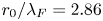 $r_0/\lambda _F=2.86$ and
 $\zeta = 1$ rearrange into a stable pentagonal structure as
 $\gamma$ is increased beyond the initial instability threshold
 $\gamma ^*=1.01\gamma _W$. (b) Drops in a ring of
 $N=20$,
 $r_0/\lambda _F=4.15$ and
 $\zeta = -1$ rearrange into a stable square as
 $\gamma$ is increased beyond the initial instability threshold
 $\gamma ^*=1.06\gamma _W$. See supplementary movie 5.

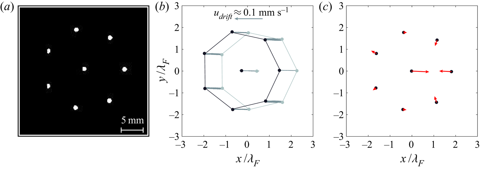
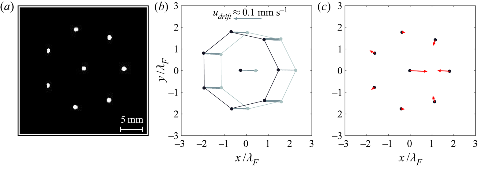
Studies investigating the stability of polygonal arrays of fluid vortices often consider the influence of an additional vortex placed at the ring's centre (see, for example, Morikawa & Swenson Reference Morikawa and Swenson1971). Although a detailed characterization of such structures is beyond the scope of this study, figure 7 and supplementary movie 6 illustrate the complex dynamics that arises when a central drop is placed in the  $N=7$,
 $r_0/\lambda _F = 1.89$,
 $\zeta = 1$ ring. Horizontal oscillations of the central drop are roughly out of phase with respect to those of the drops in the surrounding ring, resulting in a ratcheting motion that causes the entire ring to drift steadily, similar to the ratcheting dynamics exhibited by unequally sized droplet pairs (Eddi et al. Reference Eddi, Terwagne, Fort and Couder2008; Galeano-Rios et al. Reference Galeano-Rios, Couchman, Caldairou and Bush2018).
Dynamics of an  $N=7$,
 $r_0/\lambda _F = 1.89$,
 $\zeta = 1$ ring with the addition of a central droplet. (a) The static equilibrium configuration of droplets below the instability threshold,
 $\gamma ^* = 1.02 \gamma _W$. (b) The droplet positions at
 $t=0$ s (light grey) and
 $t=40$ s (black) illustrate the slow leftward drift of the entire ring at approximately
 $0.1\ \textrm {mm}\,\textrm {s}^{-1}$. (c) The instantaneous velocities of each drop, indicated by red arrows, highlight the roughly out-of-phase horizontal oscillations of the central drop with respect to the surrounding ring. See supplementary movie 6.
3. Theoretical modelling
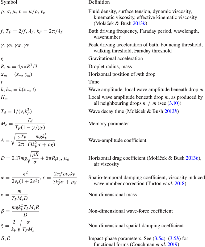
We proceed by performing a linear stability analysis of droplet rings using the variable-phase stroboscopic model of Couchman et al. (Reference Couchman, Turton and Bush2019). Definitions of relevant variables and parameters are provided in table 1. Using the dimensionless variables for position  $\bar {\boldsymbol {x}}=k_F\boldsymbol {x}$, wave height
 $\bar {h}=h/R$, and time
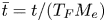 $\bar {t}=t/(T_{F}M_{e})$, the horizontal displacements
 $\bar {\boldsymbol {x}}_m$ of the
 $N$ interacting droplets are governed by the trajectory equations
 \begin{equation} \kappa\ddot{\bar{\boldsymbol{x}}}_{m}+\dot{\bar{\boldsymbol{x}}}_{m}=-\beta\sigma_{m}\mathcal{C}_{m}\nabla\bar{h}\left(\bar{\boldsymbol{x}}_{m},\bar{t}\right),\quad m=0,1,\ldots,N-1, \end{equation}
where
 \begin{equation} \bar{h}\left(\bar{\boldsymbol{x}},\bar{t}\right)=\frac{AM_{e}}{R}\sum_{n=0}^{N-1}\sigma_{n}\int_{-\infty}^{\bar{t}}\mathcal{S}_{n}\,f\left(\left|\bar{\boldsymbol{x}}-\bar{\boldsymbol{x}}_{n}\left(\bar{s}\right)\right|\right)\textrm{e}^{-\left(\bar{t}-\bar{s}\right)}\,\textrm{d}\bar{s}, \end{equation}
and
 \begin{equation} f\left(\bar{r}\right)=J_{0}\left(\bar{r}\right)\left[1+\left(\xi K_{1}\left(\xi \bar{r}\right)\bar{r}-1\right)\textrm{e}^{-\bar{r}^{-2}}\right]. \end{equation}
Definitions of relevant variables and parameters.
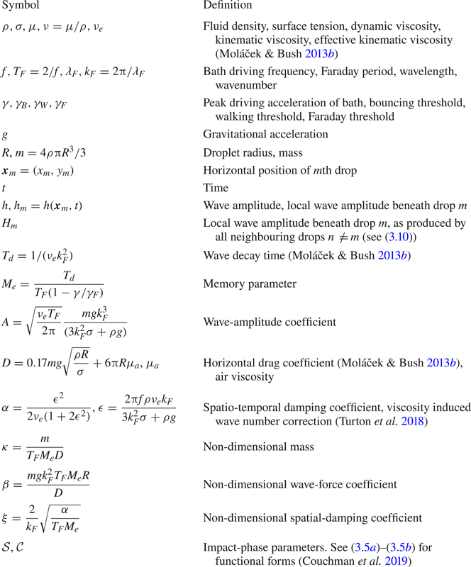
The motion of each droplet is influenced by inertia, drag, and a propulsive wave force proportional to the gradient of the underlying wave height on the bath's surface. The wave height  $h$, which has been strobed at the Faraday period
 $T_F$, is modelled as the superposition of the waves, of spatial form
 $f(r)$, generated by each of the drops’ prior impacts. We note that the wave kernel
 $f(r)$ includes a spatial damping term to account for the far-field decay of the waves, as is necessary to accurately model droplet–droplet interactions (Damiano et al. Reference Damiano, Brun, Harris, Galeano-Rios and Bush2016; Tadrist et al. Reference Tadrist, Shim, Gilet and Schlagheck2018; Turton et al. Reference Turton, Couchman and Bush2018). The parameters
 $\sigma _m = \pm 1$ are chosen to describe the relative bouncing phase of the drops:
 $\sigma _m \sigma _n = 1$ and
 $\sigma _m \sigma _n = -1$ indicate that drops
 $m$ and
 $n$ are bouncing in-phase and out-of-phase, respectively. For in-phase rings (
 $\zeta = 1$),
 $\sigma _m = 1$ for all
 $m$. For out-of-phase rings (
 $\zeta = -1$),
 $\sigma _m = (-1)^m$ for
 $m=0,1,\ldots ,N-1$.
The impact-phase parameters  $\mathcal {S}$ and
 $\mathcal {C}$, which account for the coupling between a drop's vertical and horizontal motion, are defined by
 \begin{equation} \mathcal{S}=\frac{\int_{t}^{t+T_{F}}F_{N}\left(t'\right)\sin\left({\rm \pi} ft'\right)\textrm{d}t'}{\int_{t}^{t+T_{F}}F_{N}\left(t'\right)\textrm{d}t'}, \quad \mathcal{C}=\frac{\int_{t}^{t+T_{F}}F_{N}\left(t'\right)\cos\left({\rm \pi} ft'\right)\textrm{d}t'}{\int_{t}^{t+T_{F}}F_{N}\left(t'\right)\textrm{d}t'}, \end{equation}
where  $F_N(t)$ is the vertical contact force exerted on the drop by the bath during impact. As seen in (3.4a,b),
 $\mathcal {S}$ and
 $\mathcal {C}$ are weighted averages over a Faraday period,
 $T_F$, of the sine and cosine of the phase of the bath's oscillation at which the drop impacts. The phase parameter
 $\mathcal {S}$ influences the amplitude of the wave generated at each impact while the phase parameter
 $\mathcal {C}$ influences the horizontal impulse imparted to the drop by the bath. The functional dependencies of
 $\mathcal {S}$ and
 $\mathcal {C}$ on the bath's vibrational acceleration
 $\gamma$, local-wave amplitude,
 $h_{m}=h(\boldsymbol {x}_{m},t)$, and droplet radius,
 $R$, are presented in table 2 of Couchman et al. (Reference Couchman, Turton and Bush2019). We here focus our theoretical analysis on drops of radius
 $R=0.36$ mm bouncing in a
 $(2,1)^2$ mode, as was the case for the majority of rings considered in our experiments. In this case, the impact-phase functions are
 \begin{gather} \mathcal{S}\left(\gamma,h_{m}\right) = 1-1.32\exp\left\{ -3.52\left(\gamma/g-5.73 h_{m}/R-2\right)\right\}, \end{gather}
 \begin{gather}\mathcal{C}\left(\gamma,h_{m}\right) = 1.98\exp\left\{ -2.37\left(\gamma/g-5.86 h_{m}/R-2\right)\right\}. \end{gather}
We begin by expressing (3.1) in polar coordinates with respect to the basis vectors  $(\hat {\boldsymbol {r}}_{m},\hat {\boldsymbol {\theta }}_{m})$ for each droplet. Dropping the overbars denoting non-dimensional variables for notational simplicity, we obtain
 \begin{align} &\kappa\begin{pmatrix}\ddot{r}_{m}(t)-r_{m}(t)\dot{\theta}_{m}^{2}(t)\\ r_{m}(t)\ddot{\theta}_{m}(t)+2\dot{r}_{m}(t)\dot{\theta}_{m}(t) \end{pmatrix} + \begin{pmatrix}\dot{r}_{m}(t)\\ r_{m}(t)\dot{\theta}_{m}(t) \end{pmatrix} = -\frac{AM_{e}\beta}{R}\sigma_{m}\mathcal{C}_{m} \nonumber\\ &\quad \times \sum_{n=0}^{N-1}\sigma_{n}\int_{-\infty}^{t}\mathcal{S}_{n}\frac{f'\left(d_{mn}\right)}{d_{mn}}\begin{pmatrix}r_{m}\left(t\right)-r_{n}\left(s\right)\cos\left(\theta_{m}\left(t\right)-\theta_{n}\left(s\right)\right) \\ r_{n}\left(s\right)\sin\left(\theta_{m}\left(t\right)-\theta_{n}\left(s\right)\right) \end{pmatrix}\textrm{e}^{-\left(t-s\right)}\textrm{d}s, \end{align}
where
 \begin{equation} d_{mn}=\sqrt{r_{m}^{2}\left(t\right)+r_{n}^{2}\left(s\right)-2r_{m}\left(t\right)r_{n}\left(s\right)\cos\left(\theta_{m}\left(t\right)-\theta_{n}\left(s\right)\right)}. \end{equation}
We then consider the following perturbations to an initially symmetric ring of radius  $r_0$ (see figure 1a),
 $r_{m}(t)=r_{0}+\epsilon \delta r_{m}(t)$,
 $\theta _{m}(t)=2{\rm \pi} m/N+\epsilon \delta \theta _{m}(t)$, and proceed by expanding (3.6) in orders of
 $\epsilon$.
3.1. Terms of  $\textit{O}(1)$: the set of possible rings

The  $\textit{O}(1)$ expansion of (3.6) yields two equations
 \begin{equation} 0 = \sum_{n=1}^{N-1}\zeta^{n}f'\left(2r_{0}\sin\left({\rm \pi} n/N\right)\right)\sin\left({\rm \pi} n/N\right), \end{equation}
 \begin{equation}0 = \sum_{n=1}^{N-1}\zeta^{n}f'\left(2r_{0}\sin\left({\rm \pi} n/N\right)\right)\cos\left({\rm \pi} n/N\right). \end{equation}
Recall that  $\zeta =\{ 1,-1\}$ for rings with nearest neighbours bouncing in-phase and out-of-phase, respectively, and note that
 $f'(0)=0$ which eliminates the
 $n=0$ term in each sum. Equations (3.8) and (3.9) express the requirement that the net radial and azimuthal waveforces on each drop in the ring be zero, respectively. For a given
 $\zeta$ and
 $N$, the azimuthal equation (3.9) is satisfied for all values of
 $r_0$ due to the azimuthal symmetry of the ring. However, the radial equation (3.8) will only be satisfied for a discrete set of
 $r_0$, whose values will depend on both
 $\zeta$ and
 $N$.
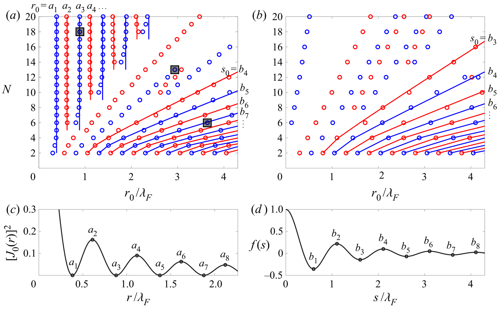
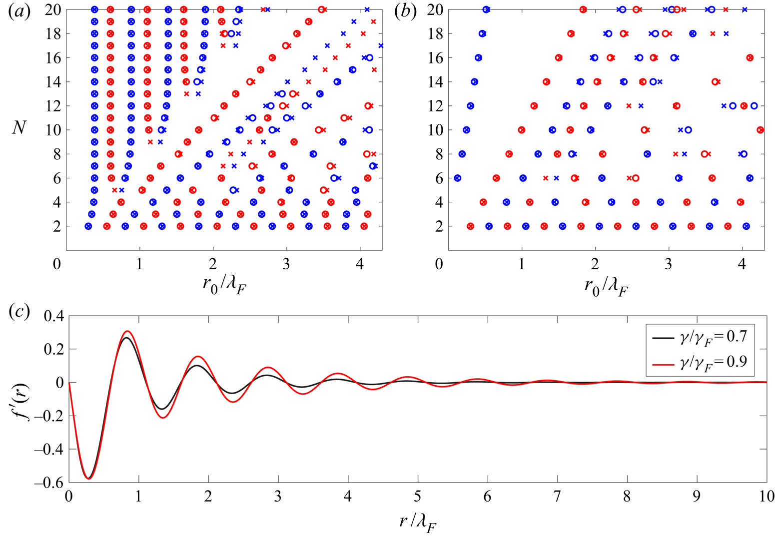
The possible radii,  $r_0$, predicted by (3.8) are plotted as a function of
 $N$ in figures 8(a) and 8(b) for rings bouncing in-phase (
 $\zeta =1$) and out-of-phase (
 $\zeta = -1$), respectively. We note that the radii
 $r_0$ are independent of the impact-phase parameters
 $\mathcal {S}$ and
 $\mathcal {C}$. However, the values of
 $r_0$ do weakly depend on the bath's vibrational acceleration
 $\gamma$, due to the dependence on
 $\gamma$ of the spatial decay parameter
 $\xi$ that appears in the wave kernel
 $f(r)$ (see (3.3)). In figure 8, we plot the possible values of
 $r_0$ at
 $\gamma /\gamma _F = 0.7$, slightly below the theoretically predicted walking threshold of a single drop,
 $\gamma _W/\gamma _F = 0.74$, which is in the vicinity of the vibrational accelerations where the rings are expected to destabilize. A comparison between the possible values of
 $r_0$ at
 $\gamma /\gamma _F = 0.7$ and
 $\gamma /\gamma _F = 0.9$ is presented in appendix A.
The possible ring radii,  $r_0$, predicted by (3.8) as a function of drop number
 $N$ for (a) in-phase
 $(\zeta = 1)$ and (b) out-of-phase
 $(\zeta = -1)$ rings. Blue and red markers correspond to rings in which each drop bounces on a minimum or maximum of the wavefield produced by the neighbouring drops (see (3.11)), respectively. Rings with side length
 $s\ll \lambda _F$ are expected to have radii corresponding to the extrema
 $a_n$ of the function
 $[J_{0}(r)]^{2}$ (see appendix B), plotted in (c). Rings with side length
 $s\gg \lambda _F$ are expected to have side lengths
 $s_0 = 2r_{0}\sin ({\rm \pi} /N)$ corresponding to the extrema
 $b_n$ of the wave kernel
 $f(s)$ (3.3), plotted in (d). The wavefields generated by the three rings boxed in panel (a) are plotted in figure 9.

To gain insight into the solutions,  $r_0$, of (3.8), consider the function
 \begin{equation} \bar{H}_{m}\left(\bar{\boldsymbol{x}}_{m},\bar{t}\right)= \frac{AM_{e}}{R}\sum_{n\ne m}\sigma_{n}\int_{-\infty}^{\bar{t}}\mathcal{S}_{n}\,f \left(\left|\bar{\boldsymbol{x}}_{m}\left(t\right)- \bar{\boldsymbol{x}}_{n}\left(s\right)\right|\right)\textrm{e}^{-\left(t-s\right)} \textrm{d}s, \end{equation}
which is the local wavefield beneath drop  $m$ that includes the wavefield contributions from all neighbouring drops
 $n\ne m$ but excludes the wavefield produced by drop
 $m$ itself. It is important to note the distinction between the closely related quantities
 $h(\boldsymbol {x}_{\boldsymbol {m}},t)$, the net wavefield beneath drop
 $m$ produced by all drops, as defined in (3.2), and
 $H(\boldsymbol {x}_{\boldsymbol {m}},t)$. Consideration of the quantity
 $H_m$ is useful because it expresses the perturbation to a given drop's local wavefield induced by its neighbours.
For drops in a symmetric ring of radius  $r$, the wavefield beneath each drop is identical. Thus, without loss of generality, we consider the perturbation to the wavefield beneath drop
 $m=0$, as produced by the neighbouring drops
 $n=1,2,\ldots ,N-1$:
 \begin{equation} \bar{H}_{0}\left(\bar{r}\right)=\frac{AM_{e}\mathcal{S}}{R} \sum_{n=1}^{N-1}\zeta^{n}f\left(2\bar{r}\sin\left( \frac{{\rm \pi} n}{N}\right)\right). \end{equation}
Note that the locations of the extrema of the function  $\bar {H}_{0}$ in (3.11) correspond to the possible radii
 $r_0$ predicted by (3.8). Thus, the solutions
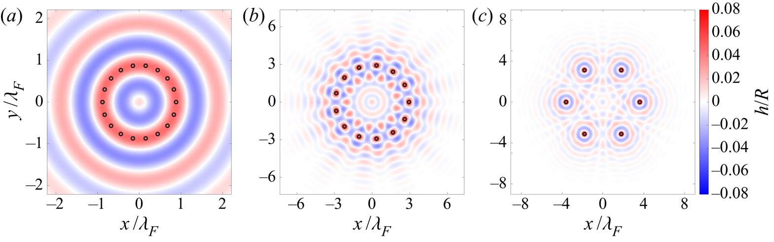
 $r_0$ in figure 8 correspond to each drop bouncing on either a maximum (red markers) or minimum (blue markers) of the wavefield produced by their neighbours at the time of impact. Figure 9 shows the wavefields generated by the three rings highlighted by grey squares in figure 8(a). We emphasize that in figure 9 we are plotting the net wavefield
 $h$, which is not to be confused with the perturbation wavefield
 $H$. Although the drops in figure 9 are seen to be bouncing on maxima of the net wavefield
 $h$, each drop is still in fact bouncing in a minimum of the wavefield
 $H$ produced by its neighbours. This is due to the fact that the large central peak in the wavefield produced by drop
 $m$ at position
 $\boldsymbol {x}_m$ overpowers the minimum in
 $H$, produced by drops
 $n\ne m$, at
 $\boldsymbol {x}_m$.
The wavefields produced at  $\gamma /\gamma _F = 0.7$ by in-phase rings with (a)
 $N=18$,
 $r_0/\lambda _F = 0.884$
 $(s_0/\lambda _F = 0.307)$, (b)
 $N=13$,
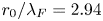 $r_0/\lambda _F = 2.94$
 $(s_0/\lambda _F = 1.41)$, and (c)
 $N=6$,
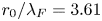 $r_0/\lambda _F = 3.61$
 $(s_0/\lambda _F = 3.61)$, boxed for reference in figure 8(a). Droplet positions are marked by black circles.

As was the case for droplet pairs (Couchman et al. Reference Couchman, Turton and Bush2019), we expect values of  $r_0$ corresponding to maxima of (3.11) to be unstable at all
 $\gamma$. Conversely, values of
 $r_0$ corresponding to minima of (3.11) are expected to remain stable up until some critical vibrational acceleration
 $\gamma ^*$. In § 3.2, we compute the threshold and type of instability for each possible solution
 $r_0$ of (3.8).
To gain further insight into the pattern of permissible radii  $r_0$ shown in figure 8, we consider two limiting cases corresponding to rings having either a large or small side length,
 $s_0 = 2r_{0}\sin ({\rm \pi} /N)$, relative to the Faraday wavelength,
 $\lambda _F$. In the limit of
 $s_0\gg \lambda _F$, each droplet in the ring is predominately influenced by its two nearest neighbours, as the wave-kernel
 $f(d)$ decays to
 ${\lesssim } 5\,\%$ of its original amplitude for inter-drop distances
 $d/\lambda _{F} \gtrsim 4$. In this limit, the ring alters its radius so that its side length corresponds to one of the stationary inter-drop spacings of a droplet pair, which occur at extrema of
 $f(s)$, as plotted in figure 8(d). The possible ring radii are then
 $r_{0}=s_{0}/(2\sin ({\rm \pi} /N))$ where
 $s_0$ satisfies
 $f'(s_0)=0$. An example of the wavefield produced by a ring in this limit is shown in figure 9(c). Note that the wave profile
 $f(s)$ in figure 8(d) is plotted at the time of impact of a drop at
 $s=0$. Therefore, for in-phase rings, side lengths corresponding to minima (
 $s_0=b_1, b_3, b_5,\ldots$) and maxima (
 $s_0=b_2, b_4, b_6,\ldots$) of
 $f(s)$ are expected to be stable and unstable, respectively. However, for out-of-phase rings, the neighbouring droplets now experience a flipped wave profile of shape
 $-f(s)$, as they impact the standing wave generated at
 $s=0$ half a cycle later. Thus, for out-of-phase rings, side lengths corresponding to maxima and minima of
 $f(s)$ are expected to be stable and unstable, respectively.
In the opposite limit,  $s_0\ll \lambda _F$, the net wavefield is well approximated by that produced by a continuous ring of wave sources with radius
 $r_0$. In appendix B, we show that for in-phase (
 $\zeta = 1$) rings with radius
 $r_0$, the resulting wavefield is
 $h(r) \propto J_{0}(r)J_{0}(r_{0})$, a radially symmetric wavefield centred on the ring's centre of mass. In this limit, the possible values of
 $r_0$ correspond to the extrema of
 $[J_{0}(r)]^{2}$, as plotted in figure 8(c). An example of the wavefield produced by a ring in this limit is shown in figure 9(a). Radii corresponding to minima (
 $r_0=a_1, a_3, a_5,\ldots$) and maxima (
 $r_0=a_2, a_4, a_6,\ldots$) of
 $[J_{0}(r)]^{2}$ are expected to be stable and unstable, respectively. A similar analysis is not possible for out-of-phase rings, as a continuous ring of wave sources of alternating phases would result in a net wavefield of zero.
We note that in the intermediate regime where  $s_0 \approx \lambda _F$, the wavefields are similar in form to those reported by Sungar et al. (Reference Sungar, Sharpe, Pilgram, Bernard and Tambasco2018) in their study of the hydrodynamic Talbot effect generated by a circular array of pillars. An example of the wavefield produced in this intermediate regime is plotted in figure 9(b).
3.2. Terms of $\textit{O}(\epsilon )$: the type and threshold of instability

At  $\textit{O}(\epsilon )$ in the expansion of (3.6), we obtain the following
 $6N \times 6N$ linear system,
 $\dot {\boldsymbol {q}}=\boldsymbol {Aq}$, as derived in appendix C
 \begin{equation} \frac{\textrm{d}}{\textrm{d}t}\underset{\boldsymbol{q}_{6N\times1}}{\underbrace{ \begin{pmatrix}\boldsymbol{\delta R}\\ \boldsymbol{\delta \varTheta}\\ \boldsymbol{\delta r}\\ \boldsymbol{\delta \theta}\\ \boldsymbol{\delta u}\\ \boldsymbol{\delta v} \end{pmatrix}}}= \underset{\boldsymbol{A}_{6N\times6N}}{\underbrace{\begin{pmatrix}-\boldsymbol{I} & \textbf{{0}} & \boldsymbol{I} & \textbf{{0}} & \textbf{{0}} & \textbf{{0}}\\ \textbf{{0}} & -\boldsymbol{I} & \textbf{{0}} & \boldsymbol{I} & \textbf{{0}} & \textbf{{0}}\\ \textbf{{0}} & \textbf{{0}} & \textbf{{0}} & \textbf{{0}} & \boldsymbol{I} & \textbf{{0}}\\ \textbf{{0}} & \textbf{{0}} & \textbf{{0}} & \textbf{{0}} & \textbf{{0}} & \boldsymbol{I}\\ \varphi\boldsymbol{U} & -\varphi\boldsymbol{V} & \varphi c_{1}\boldsymbol{I} & \textbf{{0}} & -\frac{1}{\kappa}\boldsymbol{I} & \textbf{{0}}\\ \frac{\varphi}{r_{0}^{2}}\boldsymbol{V} & \frac{\varphi}{r_{0}^{2}}\boldsymbol{W} & \textbf{{0}} & \frac{\varphi}{r_{0}^{2}}c_{2}\boldsymbol{I} & \textbf{{0}} & -\frac{1}{\kappa}\boldsymbol{I} \end{pmatrix}}}\begin{pmatrix}\boldsymbol{\delta R}\\ \boldsymbol{\delta \varTheta}\\ \boldsymbol{\delta r}\\ \boldsymbol{\delta \theta}\\ \boldsymbol{\delta u}\\ \boldsymbol{\delta v} \end{pmatrix}. \end{equation}
The  $6N\times 1$ vector
 $\boldsymbol {q}$ is composed of six
 $N\times 1$ vectors:
 $\boldsymbol {\delta R}(t)=(\delta R_{1}(t),\delta R_{2}(t),\ldots,\delta R_{N}(t))$,
 ${\boldsymbol {\delta \varTheta }}(t)=(\delta \varTheta _{1}(t),\delta \varTheta _{2}(t),\ldots ,\delta \varTheta _{N}(t))$,…,
 $\boldsymbol {\delta v}(t)=(\delta v_{1}(t),\delta v_{2}(t),\ldots ,\delta v_{N}(t))$, where
 \begin{gather} \delta R_{m}\left(t\right) = \int_{-\infty}^{t}\delta r_m \left(s\right)\textrm{e}^{-\left(t-s\right)}\textrm{d}s, \quad \delta \varTheta_{m}\left(t\right) = \int_{-\infty}^{t}\delta \theta_m \left(s\right) \textrm{e}^{-\left(t-s\right)}\textrm{d}s, \end{gather}
 \begin{gather} \delta u_{m} = \delta \dot{r}_{m}, \quad \ \delta v_{m} = \delta \dot{\theta}_{m}. \end{gather}
Each block of the matrix  $\boldsymbol {A}$ is an
 $N\times N$ matrix where
 $\boldsymbol {I}$ and
 $\textbf {{0}}$ denote the identity and zero matrices, respectively, and
 $\boldsymbol {U}$,
 $\boldsymbol {V}$ and
 $\boldsymbol {W}$ are defined in (C 25), (C 26) and (C 27) of appendix C, respectively. The scalars
 $c_1$ and
 $c_2$ are defined in (C 22) and (C 23) of appendix C, respectively, and
 \begin{equation} \varphi =-\frac{AM_{e}\beta}{4R\kappa}\mathcal{S}_{0}\mathcal{C}_{0}. \end{equation}
In (3.15),  $\mathcal {S}_{0}$ and
 $\mathcal {C}_{0}$ are the values of the phase parameters for a ring in its initial base state with radius
 $r_0$. In order to compute
 $\mathcal {S}_{0}$ and
 $\mathcal {C}_{0}$ for a given ring, we follow the procedure outlined by Couchman et al. (Reference Couchman, Turton and Bush2019). Based on (3.2), the non-dimensional local wave amplitude
 $\bar {h}_0$ beneath each drop in the ring is
 \begin{equation} \bar{h}_{0}=\frac{AM_{e}\mathcal{S}\left(\gamma,h_{0}\right)}{R}\sum_{n=0}^{N-1}\zeta^{n}f\left(2r_{0}\sin\left(\frac{{\rm \pi} n}{N}\right)\right). \end{equation}
Equations (3.5a) and (3.16) can be solved simultaneously to obtain 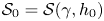 $\mathcal {S}_0=\mathcal {S}(\gamma ,h_{0})$ and
 $h_0$. Having obtained
 $h_0$,
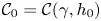 $\mathcal {C}_{0}=\mathcal {C}(\gamma ,h_{0})$ can then be computed directly using (3.5b). It will be seen that the values of
 $\mathcal {S}_{0}$ and
 $\mathcal {C}_{0}$ are significantly different for different ring geometries, as are characterized by
 $N$,
 $r_0$ and
 $\zeta$. In turn,
 $\mathcal {S}_0$ and
 $\mathcal {C}_0$ influence the ring's stability due to the dependence of the matrix
 $\boldsymbol {A}$ on
 $\varphi$ in (3.12).
We proceed by using (3.12) to determine the threshold and type of instability for each ring identified in figure 8. For a given ring, we start at  $\gamma /\gamma _F = 0.7$ and increase
 $\gamma$ progressively while tracking the evolution of the eigenvalues of
 $\boldsymbol {A}$ (3.12), as computed numerically. Below
 $\gamma /\gamma _F = 0.7$, the assumption that the drops are in a period-doubled
 $(2,1)$ bouncing mode is not expected to be valid (Wind-Willassen et al. Reference Wind-Willassen, Moláček, Harris and Bush2013). We note that, as discussed in
 $\S$3.1,
 $r_0$ depends weakly on
 $\gamma$, which obliges us to recompute the corresponding value of
 $r_0$ at each value of
 $\gamma$ using (3.8). The matrix
 $\boldsymbol {A}$ always has three eigenvalues equal to zero, reflecting the translational (
 $x, y$) and rotational (
 $\theta$) invariance of the ring. The instability threshold
 $\gamma ^*$ corresponds to the value of
 $\gamma$ at which the real part of any eigenvalue transitions from negative to positive. By analysing the eigenvector corresponding to the most unstable eigenvalue, we deduce the type of instability.
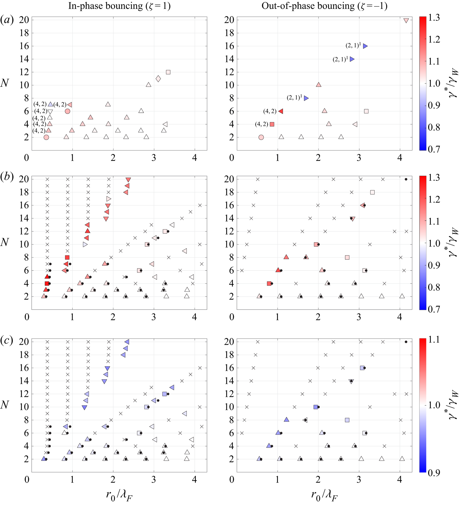
In figure 10, we compare the theoretically predicted ring radii, threshold and type of instability with our experimental data from figure 2. For comparison, we also show the theoretical predictions obtained using a constant-impact-phase model, where the phase parameters were fixed at  $\mathcal {S}_0 \mathcal {C}_0 = 0.35$, a value chosen to match the walking threshold,
 $\gamma _W$, predicted by our variable-impact-phase model. Only rings corresponding to the blue markers in figure 8 are plotted in the theoretical predictions shown in figures 10(b) and 10(c). Rings corresponding to the red markers in figure 8, indicating drops bouncing on the maxima of the wavefield produced by their neighbours, are found theoretically to be unstable already at
 $\gamma /\gamma _F = 0.7$, as anticipated. In figures 10(b) and 10(c), rings that are predicted to be unstable at the starting value of
 $\gamma /\gamma _F = 0.7$ are denoted by crosses. Rings that remain stable up to a critical vibrational acceleration,
 $\gamma ^*$, are denoted by coloured markers.
A comparison of the type and threshold of ring instability as (a) observed experimentally (reproduced from figure 2) and predicted theoretically by (b) our variable-impact-phase model and (c) a constant-impact-phase model in which the phase parameters were fixed at  $\mathcal {S}_0 \mathcal {C}_0 = 0.35$. As in figure 2, the rings are plotted as a function of the drop number
 $N$ and non-dimensional ring radius
 $r_0/\lambda _F$. The left and right columns correspond, respectively, to drops bouncing in-phase (
 $\zeta =1$) and out-of-phase (
 $\zeta =-1$) relative to their nearest neighbours. The marker colour denotes the vibrational acceleration,
 $\gamma ^*$, normalized by the walking threshold of a single drop,
 $\gamma _W$, at which the static ring is predicted to destabilize into a dynamic state. The marker shape denotes the type of instability observed: in-phase radial oscillations (
 ), out-of-phase radial oscillations (
 ), out-of-phase azimuthal oscillations (
 ), irregular rearrangements (
 ) and more complex, superposed radial and azimuthal motions (
 ). The black dots in rows (b and c) mark the rings observed experimentally in row (a) for reference, while the crosses denote rings that are already predicted to be unstable at
 $\gamma / \gamma _F= 0.7$. In the experimental data reported in (a), drops that are not bouncing in the
 $(2,1)^2$ mode, assumed in our theoretical analysis, are marked for reference. Comparison of (a) and (c) reveals that the principal shortcoming of the constant-impact-phase model is that it always predicts the onset of ring instability for
 $\gamma < \gamma _W$.

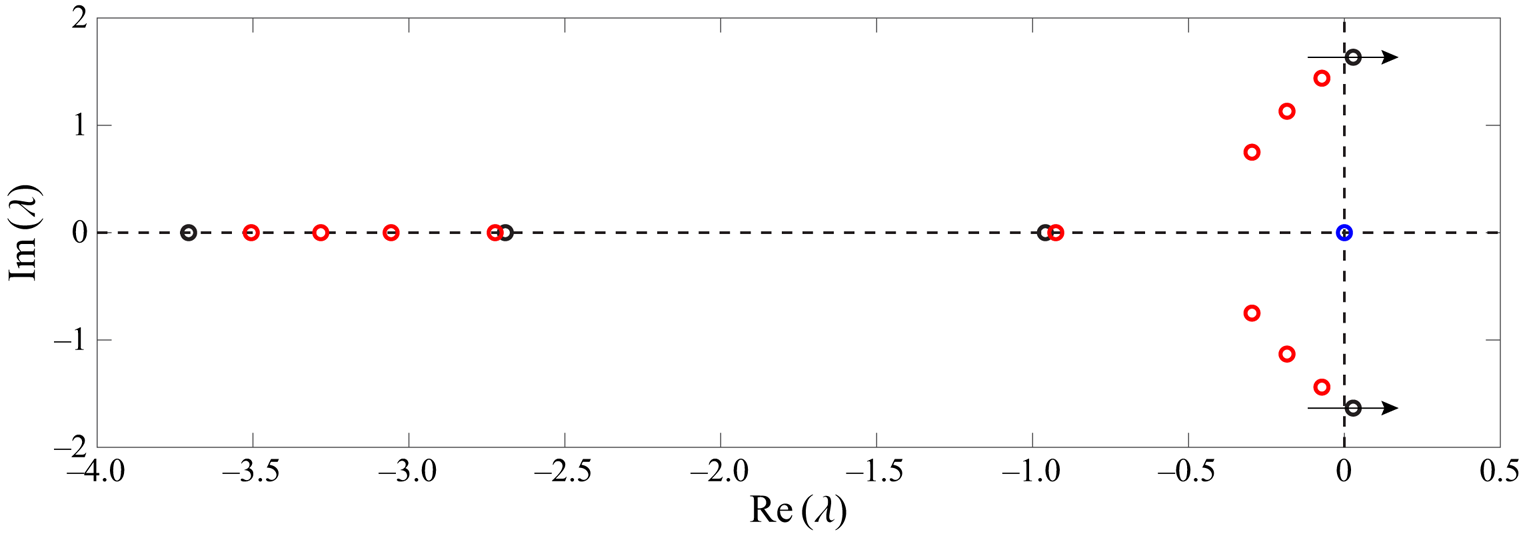
Five distinct types of instability were predicted by our linear stability analysis. In-phase radial oscillations ( , see figure 3a), out-of-phase radial oscillations (
 , see figure 3d) and out-of-phase azimuthal oscillations (
 , see figure 3c) were all characterized by a pair of complex-conjugate eigenvalues crossing the real axis at the instability threshold
 $\gamma ^*$. An example of the eigenvalue spectrum for the
 $N=5$,
 $r_0 / \lambda _F = 0.440$,
 $\zeta = 1$ ring, predicted to go unstable to in-phase radial oscillations, is shown in figure 11. Inspecting the eigenvectors corresponding to the pair of unstable eigenvalues revealed the type of oscillation. For example, in-phase radial oscillations were characterized by an eigenvector with all azimuthal components,
 $\boldsymbol {\delta \theta }$,
 $\boldsymbol {\delta v}$ and
 $\boldsymbol {\delta \varTheta }$, equal to zero and non-zero radial components
 $\delta r_1 = \delta r_2 = \delta r_3\ldots , \delta u_1 = \delta u_2 = \delta u_3\ldots$ and
 $\delta R_1 = \delta R_2 = \delta R_3\ldots$ . Out-of-phase radial oscillations were characterized by alternating signs in the radial components:
 $\delta r_1 = -\delta r_2 = \delta r_3 \ldots\,$,
 $\delta u_1 = -\delta u_2 = \delta u_3 \ldots$ and
 $\delta R_1 = -\delta R_2 = \delta R_3 \ldots$ . More complex superpositions of radial and azimuthal motion were also observed (
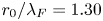
 ), corresponding to the crossing of two identical pairs of complex-conjugate eigenvalues, with corresponding eigenvectors that had both non-zero radial and azimuthal components. Finally, there were two in-phase rings,
 $N=10$,
 $r_0 / \lambda _F = 1.30$ and
 $N=17$,
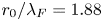 $r_0 / \lambda _F = 1.88$, for which the instability threshold corresponded to the crossing of a single, real eigenvalue. The corresponding eigenvector indicates that the drops initially move in an irregular set of directions causing the symmetric ring to break-up, which we classify as an irregular rearrangement (
 ). The nonlinear analysis required to predict the shape of the resulting aggregate is beyond the scope of our study.
The spectrum of the thirty eigenvalues of the matrix  $\boldsymbol {A}$ in (3.12) at the vibrational acceleration
 $\gamma = 1.26 \gamma _W$, just beyond the instability threshold
 $\gamma ^*$, for the ring
 $N=5$,
 $r_0 / \lambda _F = 0.440$,
 $\zeta = 1$. Black, red and blue markers indicate a single eigenvalue, two identical eigenvalues and three identical eigenvalues, respectively. The arrows indicate that, in this case, a complex-conjugate pair of eigenvalues crosses the real axis at
 $\gamma ^*$. Inspection of the corresponding eigenvectors indicates that this ring goes unstable to in-phase radial oscillations.

Our theory is found to accurately predict the stable ring radii,  $r_0$, observed experimentally. It also rationalizes why we were unable to construct rings experimentally in certain regions of the
 $(N,r_0)$ plane. For instance, in the case of
 $\zeta = -1$ rings, the theory predicts that the
 $N=4$,
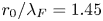 $r_0/\lambda _F = 1.45$ ring is unstable, explaining the gap apparent in the experimental data. Similarly, the theory predicts that for
 $\zeta = -1$, only one
 $N=10$ ring is stable and that no
 $N=12$ rings are stable, as found experimentally. In other cases, the theory predicts the existence of stable rings that were not found experimentally. For example, in the case of
 $\zeta = 1$ rings, we see that the theory predicts several stable rings with
 $N \ge 10$ that we did not find in the laboratory. This discrepancy is presumably due to the manner in which we created the rings: we either pushed droplets together one after another, or constructed a linear chain of droplets and then wrapped the chain around a partially submerged rod. Both techniques preferentially select certain radii based on the initial inter-drop separation distances. If the drops could be simultaneously released onto the bath in a ring formation with the desired radius, these theoretically stable states might be attainable in the laboratory.
Figure 10(b) reveals that our theoretical predictions slightly underpredict the stable ring radii,  $r_0$, with the discrepancy between theory and experiment being larger for smaller rings, but no greater than 15 %. We expect that this discrepancy may arise from our stroboscopic wave model failing to capture the influence of the radially propagating wave fronts generated at droplet impact (Eddi et al. Reference Eddi, Sultan, Moukhtar, Fort, Rossi and Couder2011b; Damiano et al. Reference Damiano, Brun, Harris, Galeano-Rios and Bush2016), that are captured by more detailed wave models (Milewski et al. Reference Milewski, Galeano-Rios, Nachbin and Bush2015; Durey & Milewski Reference Durey and Milewski2017; Galeano-Rios et al. Reference Galeano-Rios, Milewski and Vanden-Broeck2017; Galeano-Rios, Milewski & Vanden-Broeck Reference Galeano-Rios, Milewski and Vanden-Broeck2019). As shown by Galeano-Rios et al. (Reference Galeano-Rios, Couchman, Caldairou and Bush2018), these fronts influence droplet–droplet interactions when the drops are both in contact with the bath for a significant fraction of the Faraday period,
 $T_F$, and are in close proximity. For the ratcheting pairs considered by Galeano-Rios et al. (Reference Galeano-Rios, Couchman, Caldairou and Bush2018), the drops were in low energy
 $(1,1)$ and
 $(2,2)$ bouncing modes, with contact times
 $\tau _C \approx T_F/2$, and the fronts had the most notable effect on pairs with the smallest inter-drop spacing, approximately
 $\lambda _F/2$. In our experiments, the drops are in a high energy
 $(2,1)^2$ bouncing mode, with contact time
 $\tau _C \lesssim T_F/4$, and so the effect of the travelling fronts are expected to be relatively minor. Nevertheless, the discrepancy between theory and experiment being maximal for rings with radii
 $r_0 < \lambda _F$ suggests that travelling fronts may be influencing the dynamics of the most closely packed rings.
Our comparison of the theoretical predictions of a variable- and constant-impact-phase model in figure 10 highlights that variations in the vertical dynamics significantly influence the stability of droplet rings. In particular, our variable-impact-phase model predicts that rings remain stable above the instability threshold of a single drop,  $\gamma _W$, in agreement with our experimental observations. Conversely, the constant-impact-phase model, in which the impact phase is assumed to be the same for all rings, predicts that the rings destabilize below
 $\gamma _W$. The impact phase influences our stability analysis through the quantities
 $\mathcal {S}_0$ and
 $\mathcal {C}_0$ that appear in (3.15), the values of the phase parameters in the base state of each ring. As shown in figure 12,
 $\mathcal {S}_0$ and
 $\mathcal {C}_0$ change significantly with the drop number
 $N$ and ring radius
 $r_0$. By comparing figures 10(b) and 12, it is evident that the stabilization of the rings above
 $\gamma _W$ is generally due to a decrease in the product
 $\mathcal {S}_0 \mathcal {C}_0$ of the base state phase parameters. Note that in the trajectory equation (3.1),
 $\mathcal {C}$ alters the horizontal waveforce exerted on each drop; in the wavefield equation (3.2),
 $\mathcal {S}$ alters the amplitude of the wave generated at each impact. Therefore, a decrease in the product
 $\mathcal {S}_0 \mathcal {C}_0$ results in a decrease in the local wave gradient and so the lateral force experienced by each droplet at impact, thereby enhancing the ring's horizontal stability.
The base state values of the phase parameters  $\mathcal {S}_0 \mathcal {C}_0$ for each theoretically predicted stable ring in figure 10(b). Plots (a and b) correspond, respectively, to drops bouncing in-phase (
 $\zeta =1$) and out-of-phase (
 $\zeta =-1$) relative to their nearest neighbours. The product
 $\mathcal {S}_0 \mathcal {C}_0$ influences the stability of each ring through the quantity
 $\varphi$ in the linear system (3.12). In particular, rings with relatively small
 $\mathcal {S}_0 \mathcal {C}_0$ are generally found to have a higher instability threshold
 $\gamma ^*$ in figure 10(b).

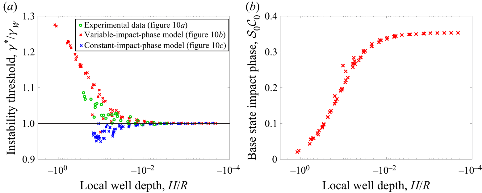
In figure 13(a), we replot the data in figure 10 as a function of the instability threshold and the depth of the wavefield well beneath each drop that is produced by its neighbours,  $H$ (3.11). As reflected by both the experimental data (green circles) and the predictions of our variable-impact-phase model (red crosses), we see that rings are more stable when droplets bounce in a deeper minimum of the wavefield produced by their neighbours. Figure 13(b) highlights that this stabilization is due to the product
 $\mathcal {S}_0 \mathcal {C}_0$ decreasing with decreasing
 $H$. The constant-impact-phase model (blue crosses), in which the phase parameters are fixed at
 $\mathcal {S}_0 \mathcal {C}_0 = 0.35$, is unable to capture this behaviour. We note further that in figure 13(a), the data points characterized by
 $H$ tending to zero and
 $\gamma ^* / \gamma _W$ tending to one correspond to loosely bound rings with a large
 $r_0$, as each drop is not being strongly influenced by its neighbours’ wavefields.
(a) The instability threshold of each ring plotted as a function of the depth of the wavefield well beneath each drop,  $\bar {H}$ (3.11), as produced by its neighbours. Green circles correspond to the experimentally observed rings in figure 10(a), red crosses to the predictions of the variable-impact-phase model in figure 10(b), and blue crosses to the predictions of the constant-impact-phase model in figure 10(c), in which
 $\mathcal {S}_0 \mathcal {C}_0 = 0.35$ is fixed. (b) The values of
 $\mathcal {S}_0 \mathcal {C}_0$ corresponding to each of the red crosses in (a), that influence the stability of each ring through the variable
 $\varphi$ (3.15) appearing in the linear system (3.12). The decrease in
 $\mathcal {S}_0 \mathcal {C}_0$ with decreasing
 $H$ is responsible for the increased stability of rings in geometries with smaller
 $H$. We note that in (a) there are more theoretical than experimental data points, as there were several theoretically predicted stable rings in figure 10 that were not considered in the laboratory.

Finally, we note that as observed in our experiments, the most common type of instability predicted was radial in-phase oscillations. The theory also predicted the majority of other types of instabilities observed experimentally, including out-of-phase radial oscillations, out-of-phase azimuthal oscillations and complex motions consisting of coupled radial and azimuthal motion. However, the instabilities predicted by the theory often occurred in slightly different regions of the  $(N,r_0)$ plane than observed in the laboratory. There are several factors that could account for this discrepancy. First, in the experimental data shown in figure 10(a), we note that for closely bound rings, the drops were in a
 $(4,2)$ bouncing mode, instead of the
 $(2,1)$ mode assumed in our theoretical model. Second, as previously discussed, our stroboscopic model neglects the influence of transient fronts, that may become important when modelling the dynamics of interacting droplets in close proximity (Galeano-Rios et al. Reference Galeano-Rios, Couchman, Caldairou and Bush2018). Third, the type of instability predicted by our stability analysis was found to be extremely sensitive to the drop size. For example, a small change in drop size from
 $R=0.36$ mm to
 $R=0.34$ mm changes the type of instability predicted for a variety of rings. For instance, orbital motion, which was not predicted theoretically with
 $R=0.36$ mm drops, emerges for in-phase
 $(N, r_0/\lambda _F)= (2, 0.30)$ and
 $(3, 0.35)$ rings composed of
 $R=0.34$ mm drops.
3.3. The nonlinear evolution of unstable rings
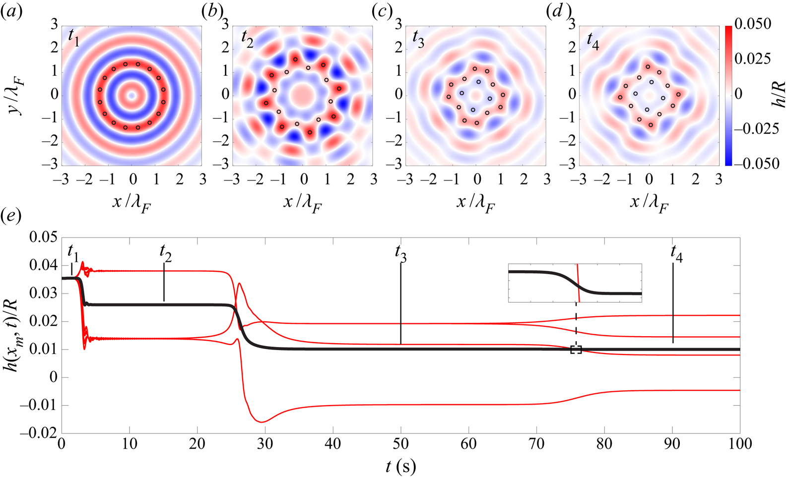
In addition to characterizing the linear stability of each ring, we performed numerical simulations using the fully nonlinear equations of motion (3.1) to investigate the behaviour of the unstable rings denoted by crosses in figure 10. At a fixed vibrational acceleration  $\gamma /\gamma _F = 0.7$, we initialized the drops in each of the unstable ring configurations shown in figure 10, imposed small velocity perturbations to each drop, and simulated the subsequent system evolution. An example of the evolution of the unstable ring
 $N=16$,
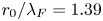 $r_0/\lambda _F = 1.39$,
 $\zeta = 1$ is shown in figure 14. We observe that the drops transition through two intermediate structures (see figure 14b,c) before finally settling into the stationary configuration shown in figure 14(d). In figure 14(e), at each instant we plot both the local wave amplitude beneath each drop,
 $h_m$, along with the local wave amplitude averaged over all drops,
 $\langle h_{m}\rangle =(1/N)\sum _{m=0}^{N-1}h_{m}$. Figure 14(e) makes clear that each re-arrangement of the drops leads to a decrease in this averaged local wave amplitude. This behaviour was generic: all of the unstable rings rearranged themselves so as to decrease
 $\langle h_{m}\rangle$ relative to the initial ring, suggesting that the underlying wavefield acts as a potential landscape that the system tries to minimize through rearrangement. A complete energetic description of the bouncing droplet system, and the utility of such a description in predicting the stability of various single- and multiple-droplet static and dynamic states, is left for future consideration.
Time evolution of the unstable ring  $N=16$,
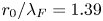 $r_0/\lambda _F = 1.39$,
 $\zeta = 1$ at the constant vibrational acceleration
 $\gamma /\gamma _F = 0.7$, as predicted by numerically simulating the trajectory equation (3.1). The drops are initialized in the ring shown in (a), evolve through the two transitional states shown in (b and c), before settling into the stationary configuration shown in (d). In (e), the evolution of the local wave amplitudes beneath each drop,
 $h_m$ (computed using (3.2)), is plotted in red, their mean
 $\langle h_{m}\rangle$ in black. The zoom box in (e) highlights that
 $\langle h_{m}\rangle$ decreases as the drops transition from state (c) to (d).

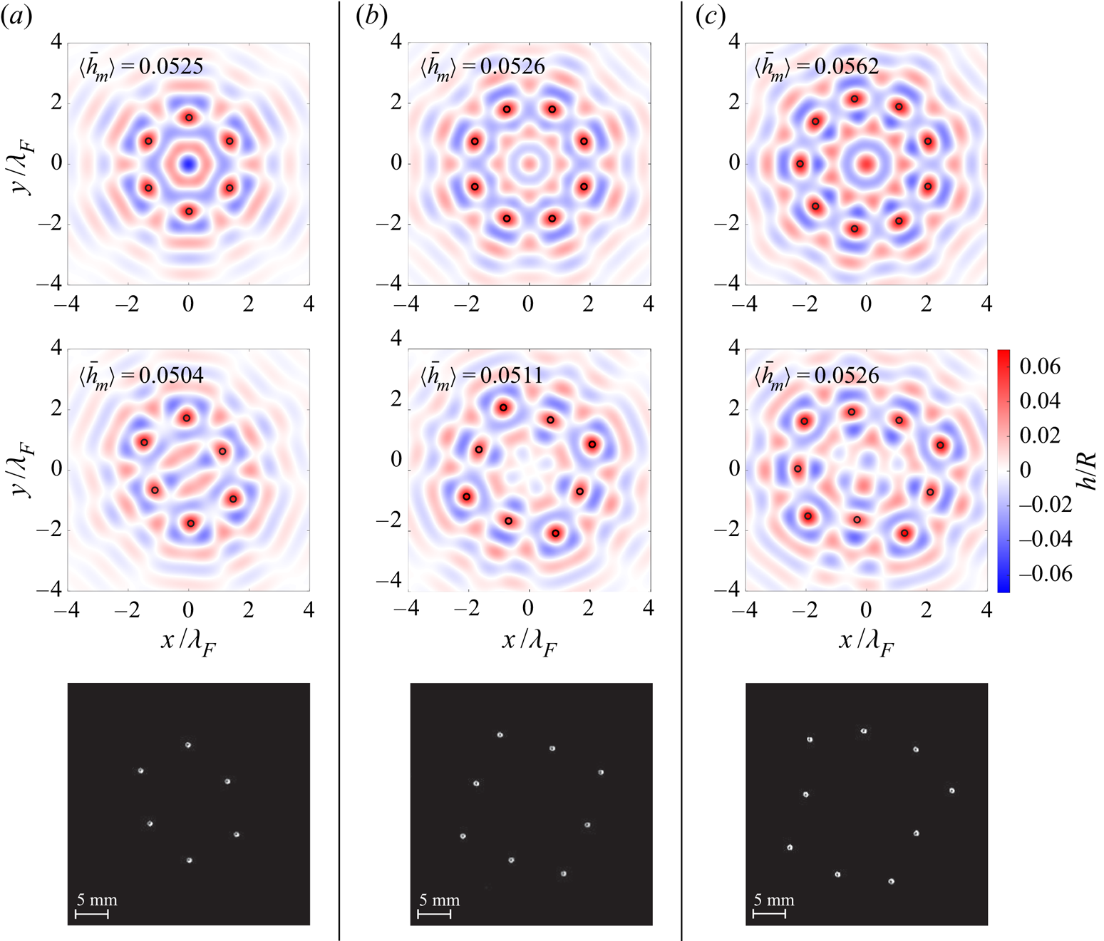
Guided by our theoretical findings, we returned to the laboratory in order to perform additional experiments to characterize the nonlinear behaviour of three of the theoretically unstable  $\zeta = 1$ rings indicated in figure 10(b):
 $(N, r_0/\lambda _F)= (6, 1.55)$,
 $(8, 1.95)$ and
 $(9, 2.18)$. As described in § 2, we partially submerged a rod in the centre of each ring to stabilize the drops as the ring was constructed. Upon removal of the rod, the drops spontaneously rearrange into a stable structure. In figure 15, we find a good agreement between the experimentally observed and theoretically predicted final stable drop configurations. In each case, once again, the drops evolve so as to reduce
 $\langle h_{m}\rangle$.
A comparison between the theoretically predicted and experimentally observed stable droplet configurations that emerge after initializing drops in the  $\zeta = 1$ unstable rings
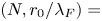 $(N, r_0/\lambda _F)=$ (a)
 $(6, 1.55)$, (b)
 $(8, 1.95)$ and (c)
 $(9, 2.18)$. The first row shows the initially unstable ring in which the drops are initialized and the second row shows the final configuration, as predicted by numerically simulating the trajectory equation (3.1). For the theoretical data, the underlying wavefield is shown along with the non-dimensional local wave amplitude averaged over all of the drops,
 $\langle \bar {h}_{m}\rangle$. The third row shows a top view of the experimentally observed stable configurations into which each unstable ring evolved.

4. Discussion
We have characterized the rings that can be constructed using  $N$ bouncing droplets, and investigated how each ring destabilizes as the bath's vibrational acceleration is increased progressively. A unique feature of our system is that the pairwise interaction force between droplets alternates between being attractive and repulsive as a function of the inter-drop distance. The result is a discrete set of possible ring radii for each drop number
 $N$, a phenomenon not seen in systems where the force field between particles decays monotonically with distance. For example, fluid point vortices are advected by the local velocity field induced by their neighbours and are found to be stable at any radius provided
 $N\le 7$ (Havelock Reference Havelock1931). For
 $N>7$, no stable rings exist. In their study of spinning magnetized disks confined to an air–fluid interface, Grzybowski et al. (Reference Grzybowski, Stone and Whitesides2000) were only able to construct stable rings for
 $N\le 5$. At each
 $N$, only a single possible radius existed corresponding to the equilibrium between two competing forces: a magnetic force attracting each disk toward a central point, and a repulsive hydrodynamic force between neighbouring disks. Our study highlights that a far greater variety of rings can be attained in the bouncing-droplet system, with rings of up to
 $N=20$ drops being found experimentally and numerous stable rings with
 $N>20$ predicted theoretically. In addition, the relative bouncing phase of the drops provides an additional degree of freedom that facilitates the construction of more complex structures.
The stability of each droplet ring depends critically on the local wave-amplitude beneath each drop, which influences the phase at which each drop impacts the bath, as highlighted in figure 13. This inference is consistent with the study of Couchman et al. (Reference Couchman, Turton and Bush2019), who found that droplet pairs in a  $(2,1)^2$ bouncing mode become progressively more stable as the inter-drop distance decreases and each drop bounces in a deeper minimum of the wavefield produced by its neighbour. For both the droplet pairs and the droplet rings considered here, the variable-impact-phase model of Couchman et al. (Reference Couchman, Turton and Bush2019) was able to capture the system's observed stability, while the constant-impact-phase stroboscopic model was not. Our study thus highlights the importance of accounting for modulations in the impact phase when modelling the interactions of multiple droplets. We note that Thomson et al. (Reference Thomson, Durey and Rosales2020b) have recently developed a weakly nonlinear analysis to study the collective vibrations in a one-dimensional lattice of bouncing droplets. A similar analysis could be developed to capture the dynamics of rings beyond the initial instability threshold, such as the amplitude of the azimuthal oscillations in figure 3(c) or the azimuthal travelling wave in figure 4.
Our study has highlighted the rich set of dynamical behaviours that may arise in multi-droplet systems and underscored the robustness of the variable-impact-phase stroboscopic model of Couchman et al. (Reference Couchman, Turton and Bush2019), opening the door for a variety of studies of the collective dynamics of multi-droplet systems. For example, by considering the relative stability of different geometries of periodic droplet lattices, one could hope to observe phase transitions between different crystalline lattice states as the bath's vibrational acceleration is increased progressively. Similarly, based on our observations that bound droplet aggregates may remain stationary at vibrational accelerations above the walking threshold of each constituent droplet,  $\gamma _W$, a system of droplets in an initially disordered ‘gaseous’ state slightly above
 $\gamma _W$ might be expected to crystallize into ordered, stationary aggregates over time.
Numerical simulations of the evolution of unstable droplet rings have shown that, at a fixed vibrational acceleration, multiple droplets evolve over time so as to minimize their averaged local wave amplitude, as highlighted in figure 14. This suggests that the wavefield on the bath's surface could be viewed as a self-induced potential landscape, a perspective that may prove valuable in characterizing the stability of other multiple-droplet structures. Campbell & Ziff (Reference Campbell and Ziff1979) catalogued all of the possible structures that could be formed out of up to  $N=50$ vortices in superfluid helium, along with their relative stability, by identifying all of the local minima in the theoretically predicted free energy landscape of the system. By developing an analogous description of the total energy of the bouncing droplet system, that includes both wave energy and drop energy, one might hope to catalogue the possible multi-droplet aggregates in a similar fashion.
Acknowledgements
J.W.M.B. gratefully acknowledges the financial support of the National Science Foundation (NSF) through grant CMMI-1727565. M.M.P.C. gratefully acknowledges the financial support of the Natural Sciences and Engineering Research Council (NSERC) through grant no. 502891. We thank Professor R. R. Rosales and Dr M. Durey for valuable discussions.
Declaration of interests
The authors report no conflict of interest.
Supplementary movies
Supplementary movies are available at https://doi.org/10.1017/jfm.2020.648.
Appendix A. Dependence of ring radii on vibrational acceleration
In figure 16, we compare the ring radii,  $r_0$, predicted by (3.8) at
 $\gamma /\gamma _F = 0.7$ and
 $\gamma /\gamma _F=0.9$. We find that as the vibrational acceleration is increased from
 $\gamma /\gamma _F = 0.7$ to
 $0.9$, the solutions that existed at
 $\gamma /\gamma _F=0.7$ do not shift significantly, but that a number of new solutions appear. Qualitatively, this can be understood by considering the dependence of the first derivative of the wave kernel
 $f'(r)$, which appears in (3.8), on
 $\gamma$, as shown in figure 16(c). As
 $\gamma$ is increased, the zeros of
 $f'(r)$ remain approximately unchanged, explaining why solutions that existed at
 $\gamma /\gamma _F = 0.7$ do not shift significantly with an increase in
 $\gamma$. However, the spatial extent of the wave form does increase significantly with increasing
 $\gamma$, explaining the appearance of new solutions at
 $\gamma /\gamma _F = 0.9$ that were not present at
 $\gamma /\gamma _F = 0.7$.
A comparison of the possible ring radii,  $r_0$, predicted by (3.8) at
 $\gamma /\gamma _F = 0.7$ (circles, reproduced from figure 8) and
 $\gamma /\gamma _F=0.9$ (crosses) for (a) in-phase
 $(\zeta = 1)$ and (b) out-of-phase
 $(\zeta = -1)$ rings. The same colour scheme is used as in figure 8. (c) A comparison of the first derivative of the wave kernel,
 $f'(r)$, that strongly influences the solutions
 $r_0$ to (3.8), at
 $\gamma /\gamma _F = 0.7$ (black line) and
 $\gamma /\gamma _F = 0.9$ (red line).

Appendix B. Approximate wavefield of closely packed rings
We here consider the wavefield produced by a ring of droplets bouncing in phase  $(\zeta = 1)$, with a side length,
 $s_0$, that is small compared to the Faraday wavelength,
 $\lambda _F$. Omitting the prefactors and overbars denoting non-dimensional variables in (3.2), the wavefield produced by a droplet ring of radius
 $r_0$ is
 \begin{equation} h\left(r,\theta\right)=\sum_{n=0}^{N-1}f\left(\sqrt{r^{2}+r_{0}^{2}-2rr_{0}\cos\left(\theta-2{\rm \pi} n/N\right)}\right). \end{equation}
To make analytical progress, we use the near-field approximation of the wave kernel in (3.3),  $f(r)\approx J_0(r)$, allowing us to make use of Graf's addition theorem
 \begin{equation} J_{0}\left(\sqrt{a^{2}+b^{2}-2ab\cos\left(\theta\right)}\right)= J_{0}\left(a\right)J_{0}\left(b\right)+2 \sum_{m=1}^{\infty}J_{m}\left(a\right)J_{m}\left(b\right)\cos\left(m\theta\right). \end{equation}
Thus,
 \begin{align} h\left(r,\theta\right)&=\sum_{n=0}^{N-1}\left[J_{0}\left(r\right)J_{0}\left(r_{0}\right)+ 2 \sum_{m=1}^{\infty}J_{m}\left(r\right)J_{m}\left(r_{0}\right)\cos\left(m\left(\theta-\frac{2{\rm \pi} n}{N}\right)\right)\right]\nonumber\\ &=NJ_{0}\left(r\right)J_{0}\left(r_{0}\right) + 2 \sum_{n=0}^{N-1}\sum_{m=1}^{\infty} J_{m}\left(r\right)J_{m}\left(r_{0}\right) \end{align}
 \begin{align} &\quad\times \left[\cos\left(m\theta\right)\cos\left(\frac{2{\rm \pi} mn}{N}\right)+\sin\left(m\theta\right)\sin\left(\frac{2{\rm \pi} mn}{N}\right)\right]. \end{align}
In the limit  $s_0 \ll \lambda _F$, we have
 $2{\rm \pi} / N \ll 1$ and can thus approximate the sum over
 $n$ in (B 4) by an integral, which yields
 \begin{align} h\left(r,\theta\right)&=NJ_{0}\left(r\right)J_{0}\left(r_{0}\right) \nonumber\\ &\quad+\frac{N}{\rm \pi}\sum_{m=1}^{\infty}\int_{0}^{2{\rm \pi}}J_{m}\left(r\right)J_{m}\left(r_{0}\right)\left[\cos\left(m\theta\right)\cos\left(mx\right)+\sin\left(m\theta\right)\sin\left(mx\right)\right]\textrm{d}x \nonumber\\ &= NJ_{0}\left(r\right)J_{0}\left(r_{0}\right). \end{align}
The wavefield produced by a ring with side length  $s_0 \ll \lambda _F$ is therefore well approximated by a radially symmetric wavefield centred on the ring's centre of mass with a radial profile proportional to
 $J_0(r)$.
Appendix C. Details of linear stability analysis
We here derive the linear system presented in (3.12). First, we substitute the perturbations  $r_{m}(t)=r_{0}+\epsilon \delta r_{m}(t)$ and
 $\theta _{m}(t)=2{\rm \pi} m/N+\epsilon \delta \theta _{m}(t)$ into (3.6) and expand in orders of
 $\epsilon$. We must separately consider the term
 $n=m$ in each sum, as the expansions for terms
 $n\ne m$ contain singularities at
 $n=m$. We then make the substitutions
 \begin{equation} \delta u_{m} = \delta \dot{r}_{m}, \quad \delta v_{m} = \delta \dot{\theta}_{m}, \end{equation}
and
 \begin{equation} \delta R_{m}\left(t\right)=\int_{-\infty}^{t} \delta r_m \left(s\right)\textrm{e}^{-\left(t-s\right)}\textrm{d}s, \quad \delta \varTheta_{m}\left(t\right) = \int_{-\infty}^{t} \delta \theta_m \left(s\right)\textrm{e}^{-\left(t-s\right)}\textrm{d}s. \end{equation}
Note that the two substitutions made in (C 2) introduce two additional differential equations
 \begin{equation} \delta\dot{R}_{m}=\delta r_{m}-\delta R_{m}, \quad \delta\dot{\varTheta}_{m}=\delta\theta_{m}-\delta\varTheta_{m}. \end{equation}
At  $\textit{O}(1)$, we obtain (3.8) and (3.9) describing the possible base radii
 $r_0$. At
 $\textit{O}(\epsilon )$, we obtain the following equations describing the evolution of the radial and azimuthal perturbations, respectively:
 \begin{align} \delta\dot{u}_{m}&=-\frac{\delta u_{m}}{\kappa}-\frac{AM_{e}\beta}{4R\kappa}\mathcal{S}_{0}\mathcal{C}_{0}\left\{ 4f''\left(0\right) \left(\delta r_{m}-\delta R_{m}\right)\right. \nonumber\\ &\quad +\sum_{n\ne m}\sigma_{m}\sigma_{n}\left[\left(M_{mn}+N_{mn}\right)\delta r_{m}+\left(M_{mn}-N_{mn}\right)\delta R_{n}\right. \nonumber\\ &\quad + \left.\left.\vphantom{4f''\left(0\right) \left(\delta r_{m}-\delta R_{m}\right)}\left(O_{mn}+P_{mn}\right)\delta\theta_{m}-\left(O_{mn}+P_{mn}\right)\delta\varTheta_{n}\right]\right\}, \end{align}
 \begin{align} \delta\dot{v}_{m}&=-\frac{\delta v_{m}}{\kappa}-\frac{AM_{e}\beta}{4R\kappa r_{0}^{2}}\mathcal{S}_{0}\mathcal{C}_{0}\left\{ 4r_{0}^{2}f''\left(0\right)\left(\delta\theta_{m}-\delta\varTheta_{m}\right)\right. \nonumber\\ &\quad +\sum_{n\ne m}\sigma_{m}\sigma_{n}\left[\left(O_{mn}-P_{mn}\right)\delta r_{m}+\left(O_{mn}+P_{mn}\right)\delta R_{n}\right. \nonumber\\ &\quad + \left.\left.\vphantom{4r_{0}^{2}f''\left(0\right)\left(\delta\theta_{m}-\delta\varTheta_{m}\right)}\left(Q_{mn}-R_{mn}\right)\delta\theta_{m}-\left(Q_{mn}-R_{mn}\right)\delta\varTheta_{n}\right]\right\}, \end{align}
where
 \begin{gather} M_{mn} = 4f''\left(2r_{0}\left|\sin\left(\frac{{\rm \pi}(m-n)}{N}\right)\right|\right)\sin^{2}\left(\frac{{\rm \pi}(m-n)}{N}\right), \end{gather}
 \begin{gather} N_{mn} = \frac{2}{r_{0}}f'\left(2r_{0}\left|\sin\left(\frac{{\rm \pi}(m-n)}{N}\right)\right|\right)\cos^{2}\left(\frac{{\rm \pi}(m-n)}{N}\right)\left|\csc\left(\frac{{\rm \pi}(m-n)}{N}\right)\right|, \end{gather}
 \begin{gather} O_{mn} = 2r_{0}\,f''\left(2r_{0}\left|\sin\left(\frac{{\rm \pi}(m-n)}{N}\right)\right|\right)\sin\left(\frac{2{\rm \pi}(m-n)}{N}\right), \end{gather}
 \begin{gather} P_{mn} = f'\left(2r_{0}\left|\sin\left(\frac{{\rm \pi}(m-n)}{N}\right)\right|\right)\sin\left(\frac{2{\rm \pi}(m-n)}{N}\right)\left|\csc\left(\frac{{\rm \pi}(m-n)}{N}\right)\right|, \end{gather}
 \begin{gather} Q_{mn} = 4r_{0}^{2}f''\left(2r_{0}\left|\sin\left(\frac{{\rm \pi}(m-n)}{N}\right)\right|\right)\cos^{2}\left(\frac{{\rm \pi}(m-n)}{N}\right), \end{gather}
 \begin{gather} R_{mn} = 2r_{0}f'\left(2r_{0}\left|\sin\left(\frac{{\rm \pi}(m-n)}{N}\right)\right|\right)\left|\sin\left(\frac{{\rm \pi}(m-n)}{N}\right)\right|. \end{gather}
The quantities  $\mathcal {S}_{0}$ and
 $\mathcal {C}_{0}$ that appear in (C 4) and (C 5) are the values of the phase parameters for a ring in its initial base state with radius
 $r_0$. The method used to compute
 $\mathcal {S}_{0}$ and
 $\mathcal {C}_{0}$ for a given ring is discussed following equation (3.15) in the main text. We note that variations in the phase parameters around the base values
 $\mathcal {S}_0$ and
 $\mathcal {C}_0$ are of
 $\textit{O}(\epsilon ^2)$ and can thus be neglected in the linear stability analysis. To see this, note that
 \begin{equation} \mathcal{S}\left[h\left(\boldsymbol{x}_{0}+\epsilon\delta\boldsymbol{x}_m\right)\right]=\mathcal{S}\left[h\left(\boldsymbol{x}_{0}\right)+\epsilon \boldsymbol{\nabla} h\left(\boldsymbol{x}_{0}\right)\boldsymbol{\cdot} \delta\boldsymbol{x}_m+O\left(\epsilon^{2}\right)\right]. \end{equation}
However, in the base state  $\boldsymbol {\nabla } h(\boldsymbol {x}_\textbf {{0}})=0$. Therefore, the impact phase only enters the linear stability analysis through the base values
 $\mathcal {S}_0$ and
 $\mathcal {C}_0$. As shown in figure 12,
 $\mathcal {S}_0$ and
 $\mathcal {C}_0$ depend on the drop number
 $N$ and the ring radius
 $r_0$. As discussed in § 3.2, these geometry-induced differences in impact phase are found to dramatically alter the instability thresholds of the rings.
We can simplify (C 4) and (C 5) by noting that
 \begin{gather} \sum_{n\ne m}\sigma_{m}\sigma_{n}O_{mn}=0, \end{gather}
 \begin{gather}\sum_{n\ne m}\sigma_{m}\sigma_{n}P_{mn}=0, \end{gather}
 \begin{gather}\sum_{n\ne m}\sigma_{m}\sigma_{n}R_{mn}=0. \end{gather}
Equations (C 13) and (C 14) hold for arbitrary values of  $r_0$ due to cancellations caused by the trigonometric functions. Equation (C 15) holds because it is equivalent to the condition in (3.8) that sets the possible base state radii
 $r_0$.
With these simplifications, and performing the summations over  $n$ for the
 $\delta r_m$ and
 $\delta \theta _m$ terms, we are left with the following six equations for each
 $m\in \{ 0,1,\ldots ,N-1\}$:
 \begin{gather} \delta\dot{R}_{m}=\delta r_{m}-\delta R_{m}, \end{gather}
 \begin{gather} \delta\dot{\varTheta}_{m}=\delta\theta_{m}-\delta\varTheta_{m}, \end{gather}
 \begin{gather} \delta\dot{r}_{m}=\delta u_{m}, \end{gather}
 \begin{gather} \delta\dot{\theta}_{m}=\delta v_{m}, \end{gather}
 \begin{gather} \delta\dot{u}_{m}=-\frac{\delta u_{m}}{\kappa}+\varphi\left(c_{1}\delta r_{m}+\sum_{n=1}^{N}U_{mn}\delta R_{n}-\sum_{n=1}^{N}V_{mn}\delta\varTheta_{n}\right), \end{gather}
 \begin{gather} \delta\dot{v}_{m}=-\frac{\delta v_{m}}{\kappa}+\frac{\varphi}{r_{0}^{2}}\left(c_{2}\delta\theta_{m}+\sum_{n=1}^{N}V_{mn}\delta R_{n}+\sum_{n=1}^{N}W_{mn}\delta\varTheta_{n}\right), \end{gather}
where
 \begin{align} c_{1}&=4f''\left(0\right)+\frac{2}{r_{0}}\sum_{n=1}^{N-1}\zeta^{n}\left[2r_{0}\,f''\left(2r_{0}\sin\left(\frac{{\rm \pi} n}{N}\right)\right)\sin^{2}\left(\frac{{\rm \pi} n}{N}\right)\right. \nonumber\\ &\quad +\left.f'\left(2r_{0}\sin\left(\frac{{\rm \pi} n}{N}\right)\right)\cos^{2}\left(\frac{{\rm \pi} n}{N}\right)\csc\left(\frac{{\rm \pi} n}{N}\right)\right], \end{align}
 \begin{align} c_{2}&=4r_{0}^{2}\left(\,f''\left(0\right)+\sum_{n=1}^{N-1}\zeta^{n}f''\left(2r_{0}\sin\left(\frac{{\rm \pi} n}{N}\right)\right)\cos^{2}\left(\frac{{\rm \pi} n}{N}\right)\right), \end{align}
 \begin{gather} \varphi =-\frac{AM_{e}\beta}{4R\kappa}\mathcal{S}_{0}\mathcal{C}_{0} \end{gather}
and
 \begin{gather} U_{mn}=\begin{cases} \dfrac{2}{r_{0}}\sigma_{m}\sigma_{n}\left[2r_{0}f''\left(2r_{0}\left|\sin\left(\dfrac{{\rm \pi}(m-n)}{N}\right)\right|\right)\sin^{2}\left( \dfrac{{\rm \pi}(m-n)}{N}\right)\right.\\ \quad \left.-f'\left(\!2r_{0}\left|\sin\left(\dfrac{{\rm \pi}(m-n)}{N}\right)\right| \right)\cos^{2}\left(\dfrac{{\rm \pi}(m-n)}{N}\right)\left|\csc\left(\dfrac{{\rm \pi}(m-n)}{N}\right) \right|\right] & n\!\ne\! m\\ -4f''\left(0\right) & n\!=\!m, \end{cases} \end{gather}
 \begin{gather} V_{mn}=\begin{cases} \sigma_{m}\sigma_{n}\sin\left(\dfrac{2{\rm \pi}(m-n)}{N}\right)\left[2r_{0}\,f'' \left(2r_{0}\left|\sin\left(\dfrac{{\rm \pi}(m-n)}{N}\right)\right|\right)\right.\\ \quad \left.+f'\left(2r_{0}\left|\sin\left(\dfrac{{\rm \pi}(m-n)}{N}\right)\right|\right) \left|\csc\left(\dfrac{{\rm \pi}(m-n)}{N}\right)\right|\right] & n\ne m \\ 0 & n=m, \end{cases} \end{gather}
 \begin{gather} W_{mn}=\begin{cases} 2r_{0}\sigma_{m}\sigma_{n}\left[\,f'\left(2r_{0}\left|\sin\left(\dfrac{ {\rm \pi}(m-n)}{N}\right)\right|\right)\left|\sin\left(\dfrac{{\rm \pi}(m-n)}{N}\right)\right|\right.\\ \quad \left.-2r_{0}f''\left(2r_{0}\left|\sin\left(\dfrac{{\rm \pi}(m-n)}{N}\right)\right|\right) \cos^{2}\left(\dfrac{{\rm \pi}(m-n)}{N}\right)\right] & n\ne m\\ -4r_{0}^{2}\,f''\left(0\right) & n=m. \end{cases} \end{gather}
Equations (C 16)–(C 21) form the linear system presented in (3.12).