2. Theoretical considerations

An appropriate starting point for our analysis is the transport equation for $\overline{({\it\delta}q)^{2}}$ in flows or flow regions where departures from local isotropy are small, viz.

The first and second terms on the left side of (2.1) represent the energy transfer and viscous diffusion of energy, respectively. The third term accounts for the inhomogeneity or non-stationarity associated with the large scales. $\overline{{\it\epsilon}}$ is defined by

where $u_{i}$ are the velocity fluctuations in the $x_{i}$ directions and the double indices convention applies. In the framework of Kolmogorov (Reference Kolmogorov1941a ), $I_{q}$ is set to zero, thus ensuring universality. Clearly, any departure from universality will arise from the term $I_{q}$ , which must be retained if turbulence is to be described accurately at all scales. At large $r$ , (2.1) reduces to the one-point energy budget equation, whereas in the limit $r\rightarrow 0$ (and after some manipulations detailed in Antonia et al. Reference Antonia, Zhou, Danaila and Anselmet2000) it reduces to the one-point transport equation of $\overline{{\it\epsilon}}$ .

For decaying grid turbulence, $I_{q}$ reflects the streamwise decay of turbulent energy, viz.

where the mean velocity $U$ is constant. When $r\rightarrow 0$ , and assuming isotropy, the transport equation for $\overline{{\it\epsilon}}$ simplifies to the equation first considered in detail by Batchelor & Townsend (Reference Batchelor and Townsend1947)

where

can be thought of as a destruction coefficient of $\overline{{\it\epsilon}}_{iso}$ , the isotropic mean energy dissipation rate. Equation (2.4) can be recast in the form (see for example Thiesset, Antonia & Djenidi Reference Thiesset, Antonia and Djenidi2014)

where

( $n$ is the power-law decay exponent of the longitudinal velocity variance, viz. $\overline{u^{2}}\sim x^{-n}$ , and $R=\overline{v^{2}}/\overline{u^{2}}$ ) is constant if $n$ is constant.

As noted in the introduction, the possible flow dependence of $C$ is of importance both in terms of turbulence modelling and also when testing for the so-called small-scale or internal intermittency effects, first introduced by K62. In the former case and the specific context of the $k{-}{\it\epsilon}$ model, the value of $C$ determines the constant in the model. It is now well accepted that the concept of a universal constant is not tenable (see for example George et al. Reference George, Wang, Wollblad and Johansson2001). In the latter case, it seems likely – as will be seen later in this section – that for the same (finite) value of $\mathit{Re}_{{\it\lambda}}$ , the value $C$ may differ in different flows. This in turn implies that the value of $S$ may differ, for nominally the same value of $\mathit{Re}_{{\it\lambda}}$ , in different flows, thus leading to an ambiguity when testing for the effect of intermittency on different small-scale statistics.

With respect to (2.7), it is evident that a large family of curves can be plotted for $S+2G/\mathit{Re}_{{\it\lambda}}$ as a function of $\mathit{Re}_{{\it\lambda}}$ in grid turbulence given the scatter in the magnitude of $n$ that exists in the literature (e.g. George Reference George1992). A power-law decay is tenable strictly when $\mathit{Re}_{{\it\lambda}}$ is constant, which corresponds to self-preservation at all scales ( $n=1$ , e.g. Meldi & Sagaut (Reference Meldi and Sagaut2013) and Djenidi & Antonia (Reference Djenidi and Antonia2015)). For most experiments, the power-law decay is only approximate and $\mathit{Re}_{{\it\lambda}}$ continues to decrease with $x$ during the decay. It is worth recalling here Speziale and Bernard’s argument (Speziale & Bernard Reference Speziale and Bernard1992) that $n=1$ is ‘the asymptotic state towards which a self-preserving isotropic turbulence is driven at high Reynolds numbers in order to resolve the fundamental imbalance between vortex stretching and viscous diffusion. In the process of resolving this imbalance, compatibility with Kolmogorov scaling is achieved for the small-scale correlations’.

On the other hand, there are flow regions, e.g. along the axis in the far field of an axisymmetric jet and the far plane wake, where self-preservation is satisfied. Provided the initial Reynolds number (based on the jet diameter $D$ and jet velocity $U_{j}$ or the cylinder diameter $d$ and free stream velocity $U_{\infty }$ ) is sufficiently large, there will be a range of $x/D$ or $x/d$ over which $\mathit{Re}_{{\it\lambda}}$ is constant, thus removing any ambiguity when plotting $S+2G/\mathit{Re}_{{\it\lambda}}$ versus $\mathit{Re}_{{\it\lambda}}$ . Since self-preservation is valid, $S$ and $2G/\mathit{Re}_{{\it\lambda}}$ do not vary with  $x$ . The consequence of self-preservation on various turbulence statistics in these two flow regions have been explored in some detail (Thiesset et al. (Reference Thiesset, Antonia and Djenidi2014) for axis of axisymmetric jet and Tang et al. (Reference Tang, Antonia, Djenidi and Zhou2015a ) far plane wake). Here we only briefly recall the main steps obtained in Thiesset et al. (Reference Thiesset, Antonia and Djenidi2014) which lead to the expression for $S+2G/\mathit{Re}_{{\it\lambda}}$ .

Along the axis of a round jet, the inhomogeneous term in (2.1) is

At large $r$ , (2.1) reduces to the one-point energy budget, viz.

since the first and second terms of the left side of (2.1) become zero when $r$ is large. In contrast to grid turbulence, the mean velocity $U$ ( ${\sim}x^{-1}$ ) decays with  $x$ . Equation (2.9) reflects the balance between $\overline{{\it\epsilon}}$ and the sum of the advection and production of the turbulent energy, the latter arising through the interaction between the normal Reynolds stresses and the mean strain rate $\partial U/\partial x$ . The jet axis region satisfies self-preservation exactly for $x/D\gtrsim 50$ , since $\mathit{Re}_{{\it\lambda}}$ does not vary with $x$ in this region (Burattini, Antonia & Danaila Reference Burattini, Antonia and Danaila2005). The limiting form of (2.1) as $r\rightarrow 0$ can be simplified using axisymmetry ( $\overline{w^{2}}=\overline{v^{2}}$ ) and local isotropy (Thiesset et al. Reference Thiesset, Antonia and Djenidi2014). The final expression is identical to (2.6), except that $C$ is now given by

Since all the flows mentioned above are of the ‘decaying’ type, it seems appropriate to consider ‘forced’ turbulence flows, which are in general less affected by finite Reynolds number or FRN effects (e.g. Antonia & Burattini Reference Antonia and Burattini2006) than decaying flows. We start by writing (2.6) in a generalized form

where $\mathscr{D}$ is exactly given by

where the term $LS(r)$ reflects the large-scale effects. Its particular form in isotropic decaying turbulence is

or, in forced turbulence,

Term $\mathscr{D}$ may further be written in the form

For decaying turbulence, and considering the expression of the large-scale term $LS\propto (u^{\prime }/L)\overline{({\it\delta}u)^{2}}$ , together with

term $\mathscr{D}$ becomes

Here, $u_{K}=({\it\nu}\overline{{\it\epsilon}})^{1/4}$ and ${\it\eta}=({\it\nu}^{3}/\overline{{\it\epsilon}})^{1/4}$ are the Kolmogorov scales. This demonstration a priori circumvents the explicit dependence of the constant $C$ on the decaying exponent $n$ (2.7), which actually depends on $\mathit{Re}_{{\it\lambda}}$ for FRN.

Note here that a similar development holds for the case when several large-scale effects coexist, such as production (due to mean velocity gradients, or coherent motion strain), turbulent diffusion, decay etc. This can be the case of non-equilibrium flows. In these cases also, the final result is that the sum of all large-scale effects behaves as $\propto 1/\mathit{Re}_{{\it\lambda}}$ for sufficiently high Reynolds numbers.

For forced turbulence, two cases will be considered.

First, an experimental box turbulence produced by pairs of opposed streams that point towards the central area of the flow. Shear turbulence, characterized by $\partial U_{i}/\partial x_{j}$ with $i\neq j$ is at this point excluded, because it is characterized by small-scale anisotropy, which is not compatible with the locally isotropic context of this derivation. Therefore, the box turbulence will be characterized by mean velocity gradients along the directions of the mean streams themselves, e.g.  $\partial U/\partial x\propto u^{\prime }/L$ , where $L$ is the scale over which the mean stream is stopped, or the scale at which the kinetic energy is injected. The large-scale term becomes

and, with a similar development as above, term $\mathscr{D}_{\mathit{forced}}$ also scales as $1/\mathit{Re}_{{\it\lambda}}$ .

Second, we consider numerically simulated forced box turbulence or SFPBT, for which the energy injection is ensured at a given scale $L_{f}$ , or a wavenumber $k_{f}\sim 1/L_{f}$ . Then, energy $E(k_{f})$ is continuously provided at the wavenumber $k_{f}$ . Term $LS_{\mathit{forced}}(r)$ is proportional to the energy at that scale times velocity gradients at that scale, so it can be written as the energy at the scale $r$ times the strain felt at that scale because of the energy injected at scale $L_{f}$ . Since the characteristic strain felt at any wavenumber $k$ is given by Danaila & Antonia (Reference Danaila and Antonia2009)

the strain at the scale $r$ becomes $s(k)\propto [E(k_{f})k_{f}^{3}]^{1/2}$ , or, in real space

which is a constant in $r$ , as it is directly given by the large-scale injection. The last step is to write $LS_{\mathit{forcing}}\sim \overline{({\it\delta}u)^{2}}s(r)$ and it is straightforward to show that

It is very reasonable to consider that the energy injected will be proportional to the typical fluctuation $u^{\prime }$ , so $u^{\prime }\sim [\overline{({\it\delta}u)^{2}}(L_{f})]^{1/2}$ . Then,

Therefore, for forced box turbulence, the constant $C$ is not zero, but is likely to be much smaller than the values of $C$ for either decaying turbulence, or when turbulence is forced over a range of scales. For example, the estimated ratio of the large-scale forcing term to $S$ for the SFPBT of Fukayama et al. (Reference Fukayama, Oyamada, Nakano, Gotoh and Yamamoto2000) is about 1.6 % at $\mathit{Re}_{{\it\lambda}}=70$ (estimated from their figure 5), while it is several orders of magnitude smaller than $S$ at $\mathit{Re}_{{\it\lambda}}=460$ for the SFPBT of Gotoh, Fukayama & Nakano (Reference Gotoh, Fukayama and Nakano2002). In this case, one expects $S+2G/\mathit{Re}_{{\it\lambda}}$ to be very nearly zero.

3. $G/\mathit{Re}_{{\it\lambda}}$

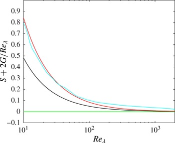
The considerations of § 2 point to $S+2G/\mathit{Re}_{{\it\lambda}}$ approaching zero at sufficiently large $\mathit{Re}_{{\it\lambda}}$ , although the approach will differ in each flow. This is summarized in figure 1. At any finite $\mathit{Re}_{{\it\lambda}}$ , grid turbulence is furthest from stationarity. One expects the SFPBT data to lie close to the $x$ axis. Given the uncertainties (e.g. noise contamination and/or inadequate spatial resolution in hot-wire measurements) in estimating $S$ and $G$ , it is unlikely that for $\mathit{Re}_{{\it\lambda}}\geqslant 300$ , one will be able to distinguish unambiguously how $S+2G/\mathit{Re}_{{\it\lambda}}$ departs from zero between different flows.

Figure 1.

Dependence of $S+2G/\mathit{Re}_{{\it\lambda}}$ (2.6) on $\mathit{Re}_{{\it\lambda}}$ in different flows: (a) grid turbulence (red), $R=0.9$ and $n=1.1$ ; (b) along the axis of a round jet (black), $R=2/3$ ; (c) ideal stationary state (green); (d) Eddy-damped quasinormal Markovian (EDQNM) simulation of decaying homogeneous isotropic turbulence (HIT) (light blue) (Meldi & Sagaut Reference Meldi and Sagaut2013).

The term $G$ , defined by (2.5), can be rewritten

where the asterisk denotes normalization by the Kolmogorov scales. If local isotropy holds, so that $\overline{{\it\epsilon}}=\overline{{\it\epsilon}}_{iso}=15{\it\nu}\overline{(\partial u/\partial x)^{2}}$ , (3.1) can be rewritten as

where ${\it\phi}_{u}^{\ast }(k_{1}^{\ast })$ is the one-dimensional spectral density of $u$ , defined such that $\int _{0}^{\infty }\!{\it\phi}_{u}(k_{1})\,\text{d}k_{1}=\overline{u^{2}}$ . If there is a departure from local isotropy, then $2G/\mathit{Re}_{{\it\lambda}}$ is estimated using

Departure from local isotropy occurs when the large-scale anisotropy is felt in the inertial range. However, when this occurs, it does not affect the results discussed in this paper. Indeed, the inertial range does not extend beyond $k^{\ast }\simeq 0.05$ , irrespective of the $\mathit{Re}_{{\it\lambda}}$ (e.g. Ishihara, Gotoh & Kaneda Reference Ishihara, Gotoh and Kaneda2009; Yoffe Reference Yoffe2012). As will be seen later (see for example figure 7), the contribution to $\int _{0}^{\infty }{k_{1}^{\ast }}^{4}{\it\phi}_{u}^{\ast }(k_{1}^{\ast })\,\text{d}k_{1}^{\ast }$ from the wavenumber range $0\leqslant k^{\ast }<0.05$ , which include the inertial range, is negligible in comparison to the contribution from the spectral region above $k^{\ast }=0.05$ . Thus, any large-scale anisotropy within the inertial range cannot affect the calculation of $G/\mathit{Re}_{{\it\lambda}}$ .

Figure 2.

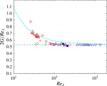
Dependence of $2G/\mathit{Re}_{{\it\lambda}}$ on $\mathit{Re}_{{\it\lambda}}$ in different flows. (a) Grid turbulence: ▹, unpublished passive grid data of Zhou & Antonia (Reference Zhou and Antonia2000); ▿, Larssen & Devenport (Reference Larssen and Devenport2011), active grid; $\times$ , Lee et al. (Reference Lee, Djenidi, Antonia and Danaila2013), passive grid; (b) axis of pipe: ▵, Rosenberg et al. (Reference Rosenberg, Hultmark, Vallikivi, Bailey and Smits2013); (c) axis of plane far-wake, ✩, Champagne (Reference Champagne1978); (c) SFPBT: ♢, Jimenez et al. (Reference Jimenez, Wray, Saffman and Rogallo1993); ○, Yeung & Zhou (Reference Yeung and Zhou1997); (d) jet axis: ▪, Lefeuvre, Djenidi & Antonia (Reference Lefeuvre, Djenidi and Antonia2015); (e) light blue curve: EDQNM (Meldi & Sagaut Reference Meldi and Sagaut2013) for HIT. The horizontal line indicates the value of 0.53.

There is ample evidence in the literature to indicate that the integrals in (3.2) or (3.3) will rapidly converge to constant values with increasing $\mathit{Re}_{{\it\lambda}}$ . This behaviour follows from the collapse of the dissipative part of ${\it\phi}_{u}(k_{1})$ when it is normalized with $u_{K}$ and ${\it\eta}$ , e.g. Saddoughi & Veeravalli (Reference Saddoughi and Veeravalli1994). This collapse does not require $\mathit{Re}_{{\it\lambda}}$ to be large (Antonia, Djenidi & Danaila Reference Antonia, Djenidi and Danaila2014), nor does it require local isotropy (LI) to be satisfied rigorously; it does, however, break down when $\mathit{Re}_{{\it\lambda}}$ is small enough, typically smaller than 40. A value as small as 20 was identified by Djenidi et al. (Reference Djenidi, Tardu, Antonia and Danaila2014).

4. Results for $S$ in a wide range of turbulent flows

Estimates of $2G/\mathit{Re}_{{\it\lambda}}$ for the flows considered in figure 1 are shown in figure 2. Also included are estimates inferred from measured spectra along the axis of a pipe by Rosenberg et al. (Reference Rosenberg, Hultmark, Vallikivi, Bailey and Smits2013) (the maximum value of $\mathit{Re}_{{\it\lambda}}$ for their measurements was 1362) and on the axis of a plane far-wake (Champagne Reference Champagne1978). Since hot-wire measurements have good temporal and spatial resolution for $\mathit{Re}_{{\it\lambda}}\leqslant 30$ , the measured spectra were used to estimate $2G/\mathit{Re}_{{\it\lambda}}$ directly in this range of Reynolds numbers. For $\mathit{Re}_{{\it\lambda}}>30$ , a uniform treatment was applied to the measured distributions of ${\it\phi}_{u}^{\ast }(k_{1}^{\ast })$ , primarily to avoid the effects of noise contamination and possible inadequate spatial resolution. The portion of the measured spectra beyond $k_{1}^{\ast }\approx 0.3$ was ignored and the distributions were extrapolated using a reference spectrum. There are now cogent analytical arguments described by Antonia et al. (Reference Antonia, Djenidi and Danaila2014), supported by strong experimental and numerical evidence at low Reynolds numbers, for extrapolating the dissipative range of the spectrum. Antonia et al. (Reference Antonia, Djenidi and Danaila2014) showed that the collapse of the Kolmogorov-normalized spectrum in the dissipative range does not hinge on local isotropy. Nor does it require the Reynolds number to be large. It is important to stress that the collapse is supported by experimental and numerical data at low Reynolds numbers (for which spatial resolution is not an issue), hence justifying the extrapolation as $\mathit{Re}_{{\it\lambda}}$ increases. The extrapolation avoids both the spatial resolution and high-frequency (measurement) noise issues as $\mathit{Re}_{{\it\lambda}}$ increases. Further, the arguments underpinning the extrapolation become all the more justifiable since there is a decreasing likelihood that the inhomogeneities in the large scales will affect the small scales when $\mathit{Re}_{{\it\lambda}}$ increases. Thus, any sufficiently well resolved numerical or experimental spectrum can be used for extrapolating the measured spectra whose dissipative range is not fully resolved. Here we used the model spectrum of Pope (Reference Pope2000) mainly for convenience. The constants were calibrated against well resolved DNS spectra (Abe, Antonia & Kawamura Reference Abe, Antonia and Kawamura2009) on the centreline of a channel flow, where the departure from LI is small and remained unchanged for all the flows used in figure 2 (details of the procedure can be found in Tang et al. (Reference Tang, Antonia, Djenidi, Abe, Zhou, Danaila and Zhou2015b ); see also Lee et al. (Reference Lee, Djenidi, Antonia and Danaila2013)). It is important to stress that the model is mainly used as a curve fit to the DNS data in the region $k^{\ast }\geqslant 0.3$ to carry out the extrapolation of the measured spectra. 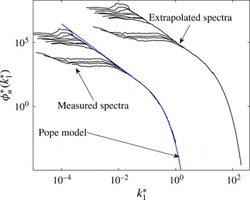Further, the use of $k^{\ast -5/3}$ in the model has not biased the values of $G/\mathit{Re}_{{\it\lambda}}$ that have been estimated from the extrapolated spectra, since, as commented earlier, the contribution from this part of the spectrum is insignificant. As an example, one set of extrapolated spectra for active grid turbulence (Larssen & Devenport Reference Larssen and Devenport2011) with $\mathit{Re}_{{\it\lambda}}$ in the range 100–1360 are shown in figure 3. For $\mathit{Re}_{{\it\lambda}}>30$ , $2G/\mathit{Re}_{{\it\lambda}}$ was estimated using the extrapolated spectra. The larger values of $2G/\mathit{Re}_{{\it\lambda}}$ at small $\mathit{Re}_{{\it\lambda}}$ in figure 2 reflect, to a large extent, the systematic departure of the Kolmogorov-normalized spectra of  $u$ , in particular the systematic increase of the spectral density in the dissipation range (e.g. Mansour & Wray Reference Mansour and Wray1994; Djenidi et al. Reference Djenidi, Tardu, Antonia and Danaila2014).

Figure 3.

Measured and extrapolated spectra for the active grid turbulence, data of Larssen & Devenport (Reference Larssen and Devenport2011) with $\mathit{Re}_{{\it\lambda}}$ in the range 100–1360. The extrapolated spectra are offset by two orders of magnitude along both $x$ and $y$ axes.

For grid turbulence, and along the axis of a round jet, $2G/\mathit{Re}_{{\it\lambda}}$ is constant ( ${\approx}0.53\pm 0.1$ ) for $\mathit{Re}_{{\it\lambda}}>70$ . For SFPBT, the constancy of $2G/\mathit{Re}_{{\it\lambda}}$ ( ${\approx}0.53$ ) is achieved at small $\mathit{Re}_{{\it\lambda}}$ ; however, it would now seem that, for this type of forced turbulence, $2G/\mathit{Re}_{{\it\lambda}}$ starts to increase slowly with $\mathit{Re}_{{\it\lambda}}$ , when the latter exceeds a value of about 300 (e.g. Ishihara et al. Reference Ishihara, Kaneda, Yokokawa, Itakura and Uno2007; Gauding Reference Gauding2014). The light blue curve, inferred from the EDQNM simulation (Meldi & Sagaut Reference Meldi and Sagaut2013), approaches the same constant value ( ${\approx}0.53$ ) as the other experimental data in figure 2 only for $\mathit{Re}_{{\it\lambda}}\approx 10^{3}$ . This slow approach, which can also be seen in figure 1, is different from that exhibited by all the other data and may reflect differences in the initial conditions between simulation and experiments.

Figure 4.

Dependence of measured values of $-S$ on $\mathit{Re}_{{\it\lambda}}$ in different flows and from two separate EDQNM simulation for decaying HIT. (a) Centreline of a fully developed channel flow (▫, blue) and pipe (✩), Antonia & Pearson (Reference Antonia and Pearson2000). (b) Along the axis of a round jet: $\bullet$ , Mi, Xu & Zhou (Reference Mi, Xu and Zhou2013); ▿, Friehe, Atta & Gibson (Reference Friehe, Van Atta and Gibson1971); $+$ , Kahalerras, Malecot & Gagne (Reference Kahalerras, Malecot and Gagne1998); ▵, (P. Burattini, private communication, 2006); ▪, Lefeuvre et al. (Reference Lefeuvre, Djenidi and Antonia2015). 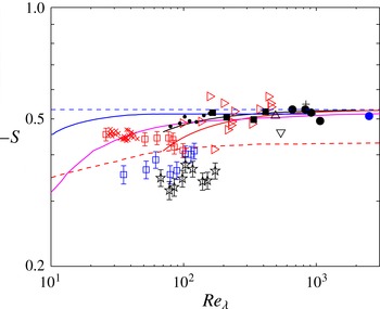(c) Grid turbulence: $\times$ , Lee et al. (Reference Lee, Djenidi, Antonia and Danaila2013); ▹, Mydlarski & Warhaft (Reference Mydlarski and Warhaft1996); ▫ (red), unpublished data of Zhou & Antonia (Reference Zhou and Antonia2000). (d) Along the axis of a plane jet, ● (black), Zhou, Antonia & Chua (Reference Zhou, Antonia and Chua2005); along the axis of the ONERA wind tunnel, ● (blue), measurements of Kahalerras et al. (Reference Kahalerras, Malecot and Gagne1998); see Bos et al. (Reference Bos, Chevillard, Scott and Rubinstein2012); blue curve, Qian (Reference Qian1994); pink and red dashed curves correspond to EDQNM of Meldi & Sagaut (Reference Meldi and Sagaut2013) and Bos et al. (Reference Bos, Chevillard, Scott and Rubinstein2012), respectively. Red and black curves, inferred from (2.6) by assuming $2G/\mathit{Re}_{{\it\lambda}}=\text{constant}$ ( ${\approx}0.53$ for $\mathit{Re}_{{\it\lambda}}>70$ ), correspond to grid turbulence, and the axis of a round jet, respectively. The horizontal line indicates the value of 0.53.

Figure 5.

Dependence of $-S$ on $\mathit{Re}_{{\it\lambda}}$ for SFPBT. ♢, Jimenez et al. (Reference Jimenez, Wray, Saffman and Rogallo1993);  $\times$ , Kerr (Reference Kerr1985); ◃, Gotoh et al. (Reference Gotoh, Fukayama and Nakano2002); ✩, Yeung & Zhou (Reference Yeung and Zhou1997); ○, Gauding (Reference Gauding2014) ( $k_{max}^{\ast }=2.53{-}4.99$ ); * (black) ( $k_{max}^{\ast }=1$ ) and * (green) ( $k_{max}^{\ast }=2$ ) correspond to Ishihara et al. (Reference Ishihara, Kaneda, Yokokawa, Itakura and Uno2007); blue curve, Qian (Reference Qian1994).

Figure 6.

Dependence of $-S$ on $\mathit{Re}_{{\it\lambda}}$ in flow between counter-rotating disks. ●, Tabeling et al. (Reference Tabeling, Zocchi, Belin, Maurer and Willaime1996);  $\times$ , Belin et al. (Reference Belin, Maurer, Tabeling and Willaime1997); blue curve, Qian (Reference Qian1994); the horizontal line indicates the value of 0.53.

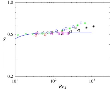
In what follows, we consider data for $-S$ obtained by various authors in a wide range of flows. Separate plots are used (figures 4–6), with the same $x$ and $y$ scales. The theoretical distribution of Qian (Reference Qian1994) is shown, as reference, on each plot. The value of 0.53 inferred from figure 2 is also shown in each plot. With the exception of the channel and pipe flows, the flows in figure 4 are of the decaying type. The red and black curves are estimated from $S+2G/\mathit{Re}_{{\it\lambda}}=C/\mathit{Re}_{{\it\lambda}}$ by assuming that $2G/\mathit{Re}_{{\it\lambda}}=\text{constant}$ ( ${\approx}0.53$ , when $\mathit{Re}_{{\it\lambda}}>70$ ). For the red curve (grid turbulence), $C$ , estimated from (2.7), is equal to 8.8 ( $n$  was 1.2 as in the experiment of Lee et al. (Reference Lee, Djenidi, Antonia and Danaila2013) and $R=0.9$ ). For the black curve (axis of axisymmetric jet), $C$ , estimated from (2.10), is equal to 4.8 ( $R=2/3$ , Thiesset et al. (Reference Thiesset, Antonia and Djenidi2014)). Although there are relatively few data available in the literature in the range $10^{2}<\mathit{Re}_{{\it\lambda}}<10^{3}$ , the trend with $\mathit{Re}_{{\it\lambda}}$ of these data provides reasonable support for the curves. The smallest values of $-S$ correspond to the centreline of the channel and the axis of the pipe (Antonia & Pearson Reference Antonia and Pearson2000). There seems little doubt that for $\mathit{Re}_{{\it\lambda}}\leqslant 200$ , where the FRN effect must be important, $-S$ can vary significantly from flow to flow. This variation is reflected in the variation of  $C$ , which in essence represents the different physical processes at large scales that contribute to the one-point energy budget in different flows. For example, one expects the large-scale contribution to the one-point energy budget in the channel and pipe by turbulent diffusion (Tang et al. Reference Tang, Antonia, Djenidi, Abe, Zhou, Danaila and Zhou2015b ). It is also evident that, for a given flow, $-S$ may depend on the initial conditions (e.g. Lavoie, Djenidi & Antonia Reference Lavoie, Djenidi and Antonia2007; Lee et al. Reference Lee, Djenidi, Antonia and Danaila2013); we also note that, for the HIT simulations of Antonia & Orlandi (Reference Antonia and Orlandi2004), Burattini, Lavoie & Antonia (Reference Burattini, Lavoie and Antonia2008), $-S$ is 0.5 for $50<\mathit{Re}_{{\it\lambda}}<60$ whereas most of the measured values are somewhat smaller at such Reynolds numbers. Despite the scatter, the data for $-S$ on the jet axis (Friehe et al. Reference Friehe, Van Atta and Gibson1971; Kahalerras et al. Reference Kahalerras, Malecot and Gagne1998; Mi et al. Reference Mi, Xu and Zhou2013) are in satisfactory agreement with the black curve. The major difficulty here is the high turbulence intensity level on the jet axis and its effect on Taylor’s hypothesis (TH). We suspect that the large values of $-S$ ( $=~0.68$ and 0.80) reported by Champagne et al. (Reference Champagne, Friehe, LaRue and Wyngaard1977) (they are not included in figure 4) were adversely affected by the corrections that were applied to TH. The two EDQNM distributions in figure 4 approach different values at large $\mathit{Re}_{{\it\lambda}}$ , possibly reflecting differences in the initial conditions. We recall once again that self-preserving HIT ( $n=1$ ) at all scales is possible only when $\mathit{Re}_{{\it\lambda}}$ is constant, regardless of its value (see Meldi & Sagaut Reference Meldi and Sagaut2013; Djenidi & Antonia Reference Djenidi and Antonia2015). In this case, $S$ can only be constant, in conformity with K41 (see the discussion in § 2).

Only SFPBT data are shown in figure 5; $-S$ is virtually constant for $\mathit{Re}_{{\it\lambda}}>20-40$ . This is in quite good accord with the analytical prediction ( $-S=0.515$ for $\mathit{Re}_{{\it\lambda}}>40$ ) of Qian (Reference Qian1994, Reference Qian2003). DNS data of Gotoh et al. (Reference Gotoh, Fukayama and Nakano2002) indicated that, for $38\leqslant \mathit{Re}_{{\it\lambda}}\leqslant 284$ , $-S$ is approximately constant ( $\simeq 0.53$ ). For $\mathit{Re}_{{\it\lambda}}=381$ and 460, $-S$ was 0.574 and 0.545, respectively, suggesting a possible small increase in $-S$ with increasing $\mathit{Re}_{{\it\lambda}}$ . This has since been confirmed by the DNS data of Ishihara et al. (Reference Ishihara, Kaneda, Yokokawa, Itakura and Uno2007), which suggest an increase of $-S$ according to (1.2) with ${\it\alpha}=0.11$ . Since this turbulence should be stationary, the increase reflects an increase of $2G/\mathit{Re}_{{\it\lambda}}$ with $\mathit{Re}_{{\it\lambda}}$ ; this issue will be discussed later in the context of figure 7.

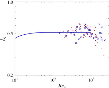
Various statistics for $\partial u/\partial x$ were presented by Tabeling et al. (Reference Tabeling, Zocchi, Belin, Maurer and Willaime1996) and Belin et al. (Reference Belin, Maurer, Tabeling and Willaime1997) for a flow of helium gas at low temperature between two counter-rotating disks over an impressively large range of $\mathit{Re}_{{\it\lambda}}$ : 150–5040 (Tabeling et al. Reference Tabeling, Zocchi, Belin, Maurer and Willaime1996) and 150–2300 (Belin et al. Reference Belin, Maurer, Tabeling and Willaime1997). In the context of this paper, these results are useful for two reasons. Firstly, $S$ has been collected in the same flow. Secondly, since the flow is of the forced type, the range of $\mathit{Re}_{{\it\lambda}}$ should be large enough to allow an exploration of ${\it\alpha}$ beyond the range of $\mathit{Re}_{{\it\lambda}}$ that is associated with FRN effects. Moisy, Tabeling & Willaime (Reference Moisy, Tabeling and Willaime1999) showed that, for this flow, $\overline{({\it\delta}u^{\ast })^{3}}/r^{\ast }$ displays a reasonable plateau, with a magnitude of about 0.77, which is quite close to Kolmogorov’s $4/5$ law, when $\mathit{Re}_{{\it\lambda}}$ exceeds 1000. Antonia & Burattini (Reference Antonia and Burattini2006) showed that, for this type of flow, $\mathit{Re}_{{\it\lambda}}\simeq 1000$ should be sufficient for FRN effects to cease being important. The data of Tabeling et al. (Reference Tabeling, Zocchi, Belin, Maurer and Willaime1996) were not included in Sreenivasan & Antonia’s compilations (Sreenivasan & Antonia Reference Sreenivasan and Antonia1997) for $S$ and $F$ , the flatness factor of $\partial u/\partial x$ , mainly because of a (slow) drop off in $S$ and $F$ beyond $\mathit{Re}_{{\it\lambda}}\simeq 700{-}800$ , which was reported to coincide with a transition to a new state of turbulence. This behaviour was reproduced in the later experiment by Belin et al. (Reference Belin, Maurer, Tabeling and Willaime1997) and the values of $S$ and $F$ seemed unaffected, at least up to $\mathit{Re}_{{\it\lambda}}\simeq 1000$ . Both sets of data for $S$ are shown in figure 6, up to $\mathit{Re}_{{\it\lambda}}\simeq 2000$ . The transitional behaviour is difficult to discern in $-S$ , but can be more easily seen in $F$ and higher-order moments of $\partial u/\partial x$ (which are not shown here). It is clear, however, that, allowing for the scatter, the Belin et al. (Reference Belin, Maurer, Tabeling and Willaime1997) data suggest, as the authors indicate, that $-S$ remains constant ( $\simeq 0.50$ ) over the whole range of $\mathit{Re}_{{\it\lambda}}$ , up to $\mathit{Re}_{{\it\lambda}}\simeq 2000$ . This is consistent with our expected behaviour (§ 2) of $-S$ when forcing is applied.

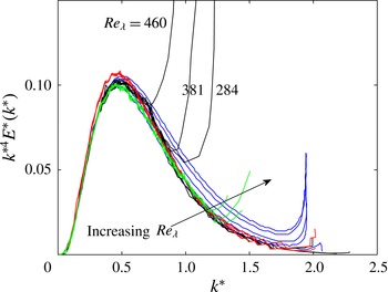
The high-wavenumber part of $k^{\ast 4}E^{\ast }(k^{\ast })$ (see blue curves in figure 7), where $E(k)$ is the 3D energy spectrum, increases systematically with $\mathit{Re}_{{\it\lambda}}$ , implying non-conformity with Kolmogorov scaling. This contrasts with the arguments put forward in Antonia et al. (Reference Antonia, Djenidi and Danaila2014), the behaviour of spectra from lower- $\mathit{Re}_{{\it\lambda}}$ DNS of SFPBT, as well as that for experimental data in a wide range of flows at comparable if not larger $\mathit{Re}_{{\it\lambda}}$ than for Ishihara et al. (Reference Ishihara, Kaneda, Yokokawa, Itakura and Uno2007). Figure 7 also shows the distributions of $k^{\ast 4}E^{\ast }(k^{\ast })$ of Gotoh et al. (Reference Gotoh, Fukayama and Nakano2002) ( $\mathit{Re}_{{\it\lambda}}=38{-}460$ ), Jimenez et al. (Reference Jimenez, Wray, Saffman and Rogallo1993) ( $\mathit{Re}_{{\it\lambda}}=35{-}168$ ) and Yeung & Zhou (Reference Yeung and Zhou1997) ( $\mathit{Re}_{{\it\lambda}}=38{-}240$ ) for SFPBT. Whilst the spectra of Jimenez et al. (Reference Jimenez, Wray, Saffman and Rogallo1993), Yeung & Zhou (Reference Yeung and Zhou1997) and Gotoh et al. (Reference Gotoh, Fukayama and Nakano2002) collapse at high wavenumbers over the range $38\leqslant \mathit{Re}_{{\it\lambda}}\leqslant 460$ , those of Ishihara et al. (Reference Ishihara, Kaneda, Yokokawa, Itakura and Uno2007) exhibit a systematic increase with $\mathit{Re}_{{\it\lambda}}$ (a similar trend has been observed by Gauding (Reference Gauding2014), private communication); this is consistent with the increase of $-S$ with $\mathit{Re}_{{\it\lambda}}$ in figure 5. It is not clear why the spectra of Ishihara et al. (Reference Ishihara, Kaneda, Yokokawa, Itakura and Uno2007) do not conform with Kolmogorov scaling, in particular with the first similarity law. Nevertheless, Ishihara et al. (Reference Ishihara, Kaneda, Yokokawa, Itakura and Uno2005, Reference Ishihara, Kaneda, Yokokawa, Itakura and Uno2007, Reference Ishihara, Gotoh and Kaneda2009) leave open the possibility, based on fitting to $k^{\ast 4}E^{\ast }(k^{\ast })$ for $k^{\ast }>0.5$ , that as $\mathit{Re}_{{\it\lambda}}\rightarrow \infty$ , $-S$ ‘approaches a constant independent of $\mathit{Re}_{{\it\lambda}}$ , but the approach may be slow’.

Figure 7.

Normalized three-dimensional DNS spectra $k^{\ast 4}E^{\ast }(k^{\ast })$ for SFPBT. Blue curves, (Ishihara et al. Reference Ishihara, Kaneda, Yokokawa, Itakura and Uno2007),  $\mathit{Re}_{{\it\lambda}}=94$ , 173, 268, 429 and 675, respectively; the arrow indicates the direction $\mathit{Re}_{{\it\lambda}}$ increases. Black curves, (Gotoh et al. Reference Gotoh, Fukayama and Nakano2002),  $\mathit{Re}_{{\it\lambda}}=38$ , 54, 70, 125, 284, 381 and 460, respectively. Red curves, (Jimenez et al. Reference Jimenez, Wray, Saffman and Rogallo1993),  $\mathit{Re}_{{\it\lambda}}=35$ , 61, 94 and 168, respectively. Green curves, (Yeung & Zhou Reference Yeung and Zhou1997),  $\mathit{Re}_{{\it\lambda}}=38$ , 90, 140, 180 and 240, respectively.

Figure 8.

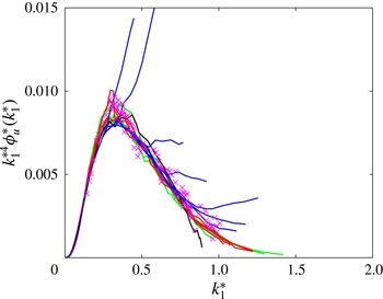
Normalized one-dimensional spectra $k_{1}^{\ast 4}{\it\phi}_{1}^{\ast }(k_{1}^{\ast })$ . Red curves, Antonia et al. (Reference Antonia, Djenidi and Danaila2014),  $\mathit{Re}_{{\it\lambda}}=41{-}140$ ; blue curves, Rosenberg et al. (Reference Rosenberg, Hultmark, Vallikivi, Bailey and Smits2013),  $\mathit{Re}_{{\it\lambda}}=109{-}788$ ; $\times$ , Larssen & Devenport (Reference Larssen and Devenport2011),  $\mathit{Re}_{{\it\lambda}}=100{-}1360$ ; black curve, DNS data of Gotoh et al. (Reference Gotoh, Fukayama and Nakano2002),  $\mathit{Re}_{{\it\lambda}}=460$ ; green curves, DNS data on the centreline of a channel flow (Abe et al. Reference Abe, Antonia and Kawamura2009),  $\mathit{Re}_{{\it\lambda}}=34{-}66$ .

Figure 9.

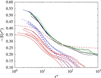
Skewness structure functions in different flows. Red curves, centreline of a fully developed channel flow, Antonia & Pearson (Reference Antonia and Pearson2000),  $\mathit{Re}_{{\it\lambda}}=33{-}120$ ( $l_{w}/{\it\eta}=0.5{-}3.0$ ). Blue dashed curves, grid turbulence, Zhou & Antonia (Reference Zhou and Antonia2000),  $\mathit{Re}_{{\it\lambda}}=26{-}99$ , ( $l_{w}/{\it\eta}=0.6{-}2.5$ ). Black curves, plane jet axis, Zhou et al. (Reference Zhou, Antonia and Chua2005),  $\mathit{Re}_{{\it\lambda}}=660{-}1067$ ( $l_{w}/{\it\eta}=1.4{-}2.3$ ). Blue solid curve, axis of a round jet, Kahalerras et al. (Reference Kahalerras, Malecot and Gagne1998),  $\mathit{Re}_{{\it\lambda}}=835$ ( $l_{w}/{\it\eta}=2.5$ ). Green curve, axis of the ONERA wind tunnel, measurements of Kahalerras et al. (Reference Kahalerras, Malecot and Gagne1998); see Bos et al. (Reference Bos, Chevillard, Scott and Rubinstein2012)  $\mathit{Re}_{{\it\lambda}}=2500$ ( $l_{w}/{\it\eta}=1.14$ ). Red dashed curve, EDQNM, Bos et al. (Reference Bos, Chevillard, Scott and Rubinstein2012),  $\mathit{Re}_{{\it\lambda}}=25\,000$ . Note that for all experimental data, $l_{w}/{\it\eta}\leqslant 3.0$ .

Contrary to figure 7, the distributions of $k_{1}^{\ast 4}{\it\phi}_{1}^{\ast }(k_{1}^{\ast })$ in figure 8, where the maximum $\mathit{Re}_{{\it\lambda}}$ is larger than in figure 7, do not exhibit any obvious dependence on $\mathit{Re}_{{\it\lambda}}$ . Notwithstanding the scatter and the peeling off at decreasing values of $k_{1}^{\ast }$ with increasing $\mathit{Re}_{{\it\lambda}}$ of some of the data, the distributions cluster together in accord with Kolmogorov scaling and the constancy of $G/\mathit{Re}_{{\it\lambda}}$ in figure 2.

We conclude this section by examining the dependence on $\mathit{Re}_{{\it\lambda}}$ of $S_{{\it\delta}u}$ , the skewness of ${\it\delta}u$ , viz. $S_{{\it\delta}u}=\overline{({\it\delta}u)^{3}}/\overline{({\it\delta}u)^{2}}^{3/2}$ , for most of the flows used in figure 4. Figure 9 highlights the relatively strong variation with $\mathit{Re}_{{\it\lambda}}$ of both the shape and magnitude of $S_{{\it\delta}u}$ , at least up to $\mathit{Re}_{{\it\lambda}}\simeq 1000$ . Whilst the variation with $\mathit{Re}_{{\it\lambda}}$ is systematic for a given flow, e.g. the centreline of the channel (solid red curves) or grid turbulence (broken blue curves), the magnitude of $S_{{\it\delta}u}$ is larger for grid turbulence than the channel flow despite $\mathit{Re}_{{\it\lambda}}$ being smaller in grid turbulence. This behaviour is of course consistent with figure 4. For all the data in figure 9, the resolution of the single hot wire, as measured by the ratio $l_{w}/{\it\eta}$ ( $l_{w}$ is the length of the wire) is adequate since $l_{w}/{\it\eta}$ remains in the range 0.5–3. For $\mathit{Re}_{{\it\lambda}}\geqslant 500$ (the plane and circular jet data as well as the Modane data at $\mathit{Re}_{{\it\lambda}}=2500$ ), the distributions of $S_{{\it\delta}u}$ seem to collapse reasonably well at small $r^{\ast }$ , up to $r^{\ast }\simeq 200$ . The rate at which $S_{{\it\delta}u}$ decreases as $r^{\ast }$ increases slows down for $r^{\ast }\geqslant 20$ , but there is no clear indication that $S_{{\it\delta}u}$ becomes constant, even for $\mathit{Re}_{{\it\lambda}}=25\,000$ . K41 requires the constant value, $(-S_{{\it\delta}u})_{IR}$ say, to be equal to $4/5C_{K}^{-3/2}$ , where $C_{K}$ is the Kolmogorov constant, i.e.  $\overline{({\it\delta}u)^{2}}=C_{K}(\overline{{\it\varepsilon}}r)^{2/3}$ . The EDQNM result of Bos et al. (Reference Bos, Chevillard, Scott and Rubinstein2012) appears to approach a plateau in the inertial range; their data suggest that $C_{K}\simeq 2.2$ , so that $(-S_{{\it\delta}u})_{IR}=0.25$ . Despite the very large $\mathit{Re}_{{\it\lambda}}$ , the plateau for $\overline{({\it\delta}u)^{2}}/(\overline{{\it\epsilon}}r)^{2/3}$ (the dashed red curve) is not yet reached (figure 3 of Bos et al. Reference Bos, Chevillard, Scott and Rubinstein2012), reinforcing Antonia & Burattini’s (Reference Antonia and Burattini2006) finding that, for decaying HIT, $\mathit{Re}_{{\it\lambda}}$ should probably exceed $10^{6}$ before the inertial range is established unequivocally.

5. Concluding discussion

Overall, figure 4 strongly supports the idea that, in each flow, $-S$ approaches the same constant value as $\mathit{Re}_{{\it\lambda}}$ increases, but this approach differs from flow to flow. This vindicates the suggestion by Thiesset et al. (Reference Thiesset, Antonia and Djenidi2014) that previous attempts at testing the $\mathit{Re}_{{\it\lambda}}$ dependence of properties of the SSM, which indiscriminately lumped together data from all types of laboratory flows, are either not meaningful or, at the very least, should be treated with caution. Further, even when the exponent is estimated from the same flow, one needs to be sure that $\mathit{Re}_{{\it\lambda}}$ is sufficiently large for the FRN effect to have disappeared. This is unlikely to be an easy task in decaying-type flows, in view of the results in Antonia & Burattini (Reference Antonia and Burattini2006).

Since the flow-dependent constant $C$ is positive (although varying from flow to flow, and possibly from position to position in a given flow), $-S$ should remain smaller than its asymptotic constant ( ${\approx}0.53$ ) until $C/\mathit{Re}_{{\it\lambda}}$ becomes negligible. As predicted by Qian (Reference Qian1994), $-S$ cannot grow unboundedly as $\mathit{Re}_{{\it\lambda}}$ increases. This is contrary to the predictions from lognormal and fractal models, (e.g. Frisch, Sulem & Nelkin Reference Frisch, Sulem and Nelkin1978; Van Atta & Antonia Reference Van Atta and Antonia1980), but is consistent with the vortex tube model of Tennekes (Reference Tennekes1968) and the heuristic model of Saffman (Reference Saffman1970).

Interestingly, the constancy of $S$ , which is equal to $S_{{\it\delta}u}$ in the limit $r^{\ast }\rightarrow 0$ , reflects complete self-preservation, or self-preservation at all scales of motion when $\mathit{Re}_{{\it\lambda}}$ is very high. In this case, $S_{{\it\delta}u}$ should collapse onto a single curve, regardless of $\mathit{Re}_{{\it\lambda}}$ , and exhibit three plateaux – one at small $r^{\ast }$ ( $S_{{\it\delta}u}=S=\text{const.}$ ), one in the inertial range ( $S_{{\it\delta}u}=(S_{{\it\delta}u})_{IR}=\text{const.}$ ), and one ( $S_{{\it\delta}u}=0$ ) at large $r^{\ast }$ ( ${>}\,L^{\ast }$ ). The constraint imposed by K41, viz. $S=\text{const.}$ , and $(S_{{\it\delta}u})_{IR}=\text{const.}$ , is therefore subsumed within this more general framework. Although figures 4, 6 and 9 support the constancy of $S$ for laboratory flows, figure 9 is a reminder that the constancy of $(S_{{\it\delta}u})_{IR}$ may be out of reach in the laboratory, at least for decaying turbulence. One expects the constancy of $S$ and $(S_{{\it\delta}u})_{IR}$ to be obtained in forced HIT, but, as illustrated in figures 5 and 7, this has yet to be confirmed by DNS for forced periodic box turbulence.

The constancy of $-S$ at sufficiently large $\mathit{Re}_{{\it\lambda}}$ implied by figures 4 and 6, which contrasts with (1.2), should not be too surprising given that the constraint of (2.6) is based on the Navier–Stokes equations. It is worth recalling, in the context of the phenomenological model of Kolmogorov (Reference Kolmogorov1962), that, over the inertial range, $\overline{({\it\delta}u)^{3}}$ is constrained to vary proportionately to $r$ , provided $\mathit{Re}_{{\it\lambda}}$ is sufficiently large. All small-scale intermittency models have had to satisfy this constraint. Future research may be able to verify that normalized higher-order moments of $\partial u/\partial x$ , e.g. the flatness factor ( $F=\overline{(\partial u/\partial x)^{4}}/\overline{(\partial u/\partial x)^{2}}^{2}$ ) of $\partial u/\partial x$ , may, like $-S$ , be also bounded at sufficiently large $\mathit{Re}_{{\it\lambda}}$ , once the appropriate constraint derived from the Navier–Stokes equations is understood. Such a possibility was considered by Qian (Reference Qian1986).