1. INTRODUCTION
Gyros have been successfully used to determine system orientation in many applications. But it is well known that gyros suffer from error drift (Pandit et al., Reference Pandit and Zhang1986; Van Dierendonck et al., Reference Van Dierendonck and Brown1969), which is a time-variant low frequency bias and will result in considerable orientation error for a long-term operation. For low cost gyros, such as MEMS gyros, the drift rate can reach the level of several degrees per second; even for the best gyros (which are very expensive), the accumulated errors cannot be ignored. On the other hand, accelerometer and magnetometer sensors together can also be used to determine orientation (Gebre-Egziabher et al., Reference Gebre-Egziabher, Elkaim, Powell and Parkinson2000). Accelerometer and magnetometer sensors do not have long-term drift effects, while both of them suffer from big short term noise. So in many applications of attitude and heading reference systems (AHRS), the integration of the IMU, namely the gyro triad and accelerometer triad, with magnetometers is used to provide robust orientation solutions.
Marins et al. (Reference Marins, Yun, Bachmann, McGhee and Zyda2001) presented a quaternion based method to integrate the IMU and magnetometer sensors. In their paper, three body angular rates and four quaternion elements were used to express orientation and were selected as the states of Kalman filter. This method needs to model the angular motion of the body, and in that paper the body angular rates were modelled as an exponential function. Emura et al. (Reference Emura and Tachi1994a) proposed a similar quaternion based AHRS algorithm, but in their paper the body angular rates were modelled to be constant; while in the paper of Azuma et al. (Reference Azuma and Bishop1994), the body angular rates were modelled to be an angular acceleration constant. Furthermore, the quaternion-based method suffers from the nonlinear problem, because the differential quaternion equation is nonlinear itself. Marins et al (Reference Marins, Yun, Bachmann, McGhee and Zyda2001) proposed a quaternion convergence algorithm to solve the nonlinear problem, which increased the computational efficiency.
Emura et al. (Reference Emura and Tachi1994b) proposed an Euler angle based method for the integrated AHRS, in which three body angular rates and three Euler angle components were used to express orientation and were chosen as the Kalman filter states. As the quaternion based method, the method proposed in that paper also needs to model the body angular motion, and the body angular rates were modelled to be constant. Koifman et al (Reference Koifman and Merhav1990) also presented an Euler angle based method for AHRS, but in their model the body angular rates were modelled according to the aircraft's dynamics, which could provide a more accurate orientation solution, but precise modelling of the body angular motion is quite difficult for general applications. The Euler angle based method uses the Euler angle integration kinematics (Cooke et al., Reference Cooke, Zyda, Pratt and McGhee1993), which is a nonlinear derivative equation, so the Euler angle based method also suffers from the nonlinear problem.
Foxlin (Reference Foxlin1996) presented an Euler angle error based method to integrate IMU and magnetometer sensors, and Setoodeh et al. (Reference Setoodeh, Khayatian and Farjah2004) used a similar method to achieve such integration for the AHRS. In their papers, three Euler angle errors and three gyro biases were used as the states of Kalman filter, and the estimated states were used to correct the Euler angles and to compensate gyro drifts, respectively. Being different from all of the methods above, their methods need not model the body angular motion. But similar to all the other methods mentioned above, their system equations also suffer from the nonlinear problem.
In this paper, three Euler angle errors, three gyro biases and three gyro scale factors are used as the states of Kalman filter, but in this work the three Euler angle errors are not used to express the body frame (b) errors, but are instead used to express the local level frame (l frame) errors. The definition to the Euler angle errors used in this paper will be elaborated in Section 3. The benefit of the proposed method is that the nonlinear problem is avoided and eventually the computational efficiency is improved.
According to the INS terminology, attitude represents the set of yaw, pitch and roll; while in the field of AHRS, attitude generally only expresses the set of pitch and roll, and yaw is expressed using another term heading. To avoid such confusion, in this paper, the term orientation is used to express the whole set of yaw, pitch and roll; attitude is just used for the set of pitch and roll; heading is used to express yaw angle.
2. ORIENTATION DETERMINATION
It is well known that three gyros could be used to determine the orientation of moving objects. And the arrangement of accelerometer triad and magnetometer triad could also be used to determine orientation. The following subsections will demonstrate the methods used to calculate orientation using gyros only and using the combination of accelerometers and magnetometers.
2.1. Gyro Based Orientation Determination
The quaternion based method (Savage, Reference Savage1998) is used to determine orientation using gyros outputs. The quaternion update formula could be expressed as:

where q b(m)l(m) is the orientation quaternion at time t m, q b(m−1)l(m−1) the orientation quaternion at time t m−1, while q l(m−1)l(m) and q b(m)b(m−1) represent the l frame orientation update quaternion and the b frame orientation update quaternion in the interval t m−1 to t m, respectively.
2.1.1. Body Frame Orientation Update
If the rotation vector of the b frame from t m−1 to t m is expressed as  , the b frame orientation update quaternion can be written as:
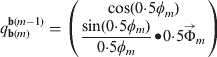
where ɸ m is the magnitude of the rotation vector and is defined as:
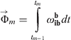
where ω ibb is the b frame rotation angular rate which is sensed by the gyros mounted in the b frame. In equation (3), the coning compensation is ignored, given the fact that low-cost MEMS devices are used for the AHRS considered here.
2.1.2. Local Level Frame Orientation Update
If the rotation vector for the local level frame from t m−1 to t m is expressed as  , the local level frame orientation update quaternion can be written as:
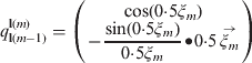
where ξ m is the magnitude of the rotation vector  defined as:

where ω ill is the rotation angular rate of the local level frame relative to the inertial frame which is composed of the Earth's self-rotation and the rotation of the local level frame relative to the Earth.
2.2. Accelerometer and Magnetometer Based Orientation Determination
In this IMU/magnetometer integrated AHRS, accelerometers and magnetometers are used together to determine orientation which is compared with the orientation computed from the gyro outputs and the orientation differences are used as the observations in the Kalman filtering to estimate the orientation errors as well as the gyro drifts and gyro scale factors.
2.2.1. Attitude Determination
Accelerometers are used to measure gravity, and the corresponding outputs from accelerometers are used to perform levelling. By comparing the outputs of three orthogonal accelerometers with gravity, the tilt angles between the b frame and the l frame can be determined. The gravity sensed by accelerometers in the b frame is expressed as A b, while the gravity in the l frame is written as A l. A b and A l are defined as:


The relationship between A b and A l is formulated as:

where C lb is the orientation transformation matrix (Savage, Reference Savage2000) from the l frame to the b frame, which can be formulated as:

where C 1,C 2 and C 3 are defined as:
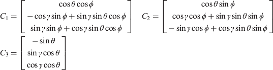
where ɸ, θ and γ represent heading, pitch and roll respectively.
Substituting equations (6), (7) and (9) into equation (8), the following formula determining the tilt angles, namely pitch and roll, can be derived as:


2.2.2. Heading Determination
Caruso (Caruso, Reference Caruso2000) proposed a method to determine the heading using geomagnetic measurements. Assuming m x, my and m z to be the components of geomagnetism in the b frame, which are measured from magnetometers, the horizontal components of geomagnetism in the l frame, X h and Y h, can be expressed as:


According to equations (12) and (13), the heading can be determined to be:

3. SYSTEM INTEGRATION SCHEME
A Kalman filter is developed for the AHRS, integrating the gyro derived orientation and the orientation determined by accelerometer and magnetometer.
As mentioned in Section 1, the customary integration methods are subject to two annoyances, modelling the body angular motion and the nonlinear problem. So the construction of this Kalman filter is based on two principles:
• Error state model, rather than full state model, is used in this Kalman filter. In the full state model, modelling of the body angular motion is required, because the body angular rates are included in the states of Kalman filter, as Koifman et al. (Reference Koifman and Merhav1990), Azuma et al. (Reference Azuma and Bishop1994), Emura et al. (Reference Emura and Tachi1994a), Emura et al. (Reference Emura and Tachi1994b) and Marins et al. (Reference Marins, Yun, Bachmann, McGhee and Zyda2001) did. Through adopting the error state model in the Kalman filtering, the difficulty and complexity of modelling the body angular motion is avoided, because the body angular rates are excluded from the Kalman filtering states.
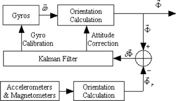
• Euler angle errors expressing the l frame errors, rather than the Euler angle errors expressing the b frame errors, is used in this Kalman filter. The differential equation for the Euler angle errors expressing the b frame errors is nonlinear; while the differential equation for the Euler angle errors expressing the l frame errors is linear, which will be shown in the following subsection. So this frame transition converts the nonlinear problem of orientation determination into a linear problem. The system schematic diagram is shown in Figure 1.
Schematic diagram for IMU and magnetometer integrated AHRS.

3.1. System Error Model
In the work of Foxlin (Reference Foxlin1996), Euler angle error  represents the orientation difference between the computed body frame (
 ) and the true body frame (b), and equals to the rotation vector from the b frame to the frame. It is well known that the differential equation of the Euler angles is nonlinear (Cooke et al., Reference Cooke, Zyda, Pratt and McGhee1993), so the differential equation of the Euler angle error is also nonlinear.
Inspired by the Psi-angle error propagation equation (Goshen-Meskin, Reference Goshen-Meskin and Bar-Itzhack1992) of the inertial navigation system (INS), the following linear model for the AHRS is obtained. It is well known that the INS Psi-angle error propagation equation is linear (Goshen-Meskin, Reference Goshen-Meskin and Bar-Itzhack1992). Removing the position error, the Psi-angle error  represents the orientation difference between the platform frame, and the local level frame (l); here the platform frame is a terminology in INS and could be viewed as the computed local level frame (
 ). Thus, equals to the rotation vector from the l frame to the frame. So is the Euler angle error and expresses the l frame error arising from the gyro errors.
As the computational errors are negligible, both and , in essence, come from the same gyro errors. So they should have a deterministically quantitative relationship, which will be derived in the next subsection. In fact, the linear differential equation of is just a linear expression for the nonlinear differential equation of , because both these errors come from the same source, namely the gyro errors, in essence. So the Psi-angle error equation could also be used to express the error propagation characteristics of the AHRS.
Referred to the INS error model (Goshen-Meskin, Reference Goshen-Meskin and Bar-Itzhack1992), differential equation of the Euler angle error expressing the l frame error for the AHRS could be expressed as:
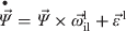
where is the Euler angle error expressing the l frame error, and  is the rotation rate of the l frame relative to the inertial frame expressed in the l frame, and
 is the errors of gyros expressed in the l frame. The gyro errors include constant bias and scale factor error, which are defined as G b and G s respectively. So the matrix form of equation (15) could be written as:

where v is the process noise vector and x is the error state vector defined as:

where x 1, x 2, x 3 are defined as:

where Ψ NΨ E ΨD are the elements of the orientation error , and G bxG byG bz are the elements of gyro bias G b expressed in the b frame, and G sxG syG sz are the elements of the gyro scale factor G s expressed in the b frame.
The system matrix A is defined as:
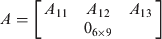
where A 11A 12A 13are defined as:
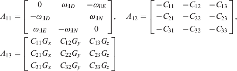
where ω il represents the rotation rate of the l frame relative to the inertial frame; C ij is the element of the direction cosine matrix C bl; G represents the angular increment measured by gyros; N, E and D represent the elements’ subscripts of vectors in the l frame; x, y and z represent the subscripts for the elements in the vectors in the b frame.
3.2. System Observation Model
Herein, the Euler angle errors expressing the b frame errors, which equal to the differences between the angles calculated from gyro outputs and the angles calculated from the outputs of accelerometers and magnetometers, are chosen as observations. While the Euler angle errors used in the system error model defined by equation (15) expresses the l frame errors, so the relationship between the Euler angle errors expressing the b frame errors and the Euler angle errors expressing the l frame errors should be determined first.
Generally, there are three methods to express orientation, namely Euler angles, direction cosine matrix, and quaternion. The relationship between Euler angles and direction cosine matrix could be written as:


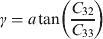
where ɸ, θ and γ are yaw, pitch and roll respectively, and C ij is the elements of the direction cosine matrix,C bl.
With the derivatives for both sides of equations (19), (20), (21), the following formula can be derived:
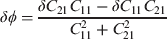
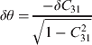
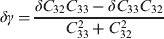
where δɸ, δθ and δγ are the Euler angle errors expressing the b frame errors and δC ij is the elements of the error matrix of the direction cosine matrix, namely δC bl.
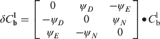
Given the Euler angle errors expressing the l frame errors, namely ψ Nψ Eψ D, the expression of δC blwill be derived as follow:
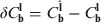
where  is the direction cosine matrix from the b frame to the
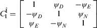
 frame, while C bl is the direction cosine matrix from the b frame to the l frame. could be formulated as:

where  is the direction cosine matrix from the l frame to the
 frame, and could be expressed as:
Finally, the error matrix of the direction cosine matrix could be written as:
Because C bl is an orthogonal matrix, so the following formula can be obtained:

Substituting equations (9), (28), and (29) into equations (22), (23), (24), the relationship between the Euler angle errors expressing the b frame errors and the Euler angle errors expressing the l frame errors could be expressed as:
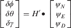
where H′ is defined as:
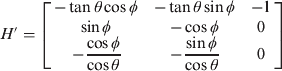
where δɸ,δθ and δγ are the Euler angle errors expressing the b frame errors, and ψ N, ψE and ψ D are the Euler angle errors expressing the l frame errors. So the observation matrix H could be written as:

And the observation equation could be formulated as:

where y is the observation vector and w is the observation noise vector. y is defined as:

4. EXPERIMENTAL TEST
This section presents the test results that demonstrate the performance characteristics of the proposed method to integrate the IMU and magnetometer for the AHRS. The data were collected from Xsens MTi, which is a miniature Attitude and Heading Reference System (AHRS) comprised of three MEMS gyros, three MEMS accelerometers and three low cost magnetometers. Two different test scenarios were implemented: a stationary test and an in-motion test. During the stationary test, Xsens MTi was fixed on a table stationary relative to the earth and the raw measurements data were collected. In the in-motion scenario, the Xsens MTi was mounted on a moving body which was controlled to move to experience heading, pitch and roll manoeuvres, and the corresponding raw measurements data were collected.
The orientation accuracy was assessed by evaluating the “absolute” accuracy and by analyzing the residuals of the orientation solution of the Kalman filtering. The absolute accuracy was evaluated using the orientation outputs of the commercial Xsens MTi as a reference. To obtain additional insight into the orientation errors, the residuals of the orientation solution of the Kalman filtering are calculated as follows:

where y is the observation, H is the observation matrix and  is the estimated value of the state vector from the Kalman filter. The main advantage of residual analysis is its independence from the reference noise.
4.1. Stationary Test Results
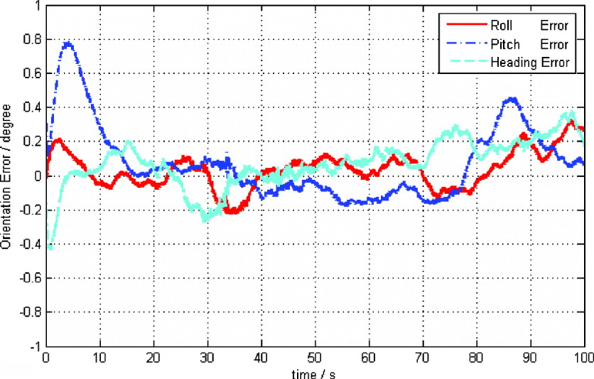
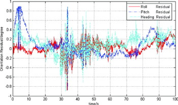
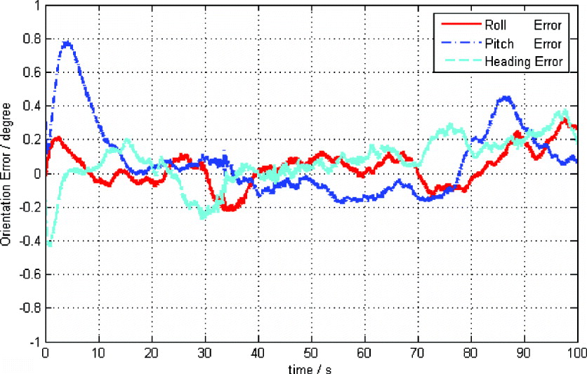
In the stationary test scenario, the system was fixed on a static table to perform stationary test. Figure 2 illustrates the roll, pitch and heading errors in the stationary test. Figure 3 illustrates the roll, pitch and heading residuals, respectively, of the Kalman filtering in the stationary test. Table 1 shows the RMS values of the orientation errors and residuals. The results presented in Figures 2, 3 and Table 1 indicate that the RMS values of the orientation errors are below 20 arcminutes in the stationary test.
Orientation errors in the stationary test.
Orientation residuals in the stationary test.

Stationary test error analysis.

4.2. In-motion Test Results
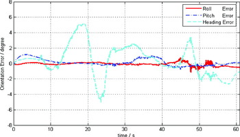
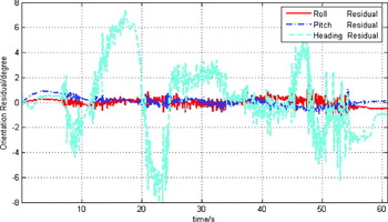
In the in-motion test scenario, the tested system was mounted on a moving body to perform the in-motion test. Figure 4 illustrates the roll, pitch and heading errors, respectively, in the in-motion test. Figure 5 illustrates the roll, pitch and heading residuals, respectively, of Kalman filtering in the in-motion test. Table 2 shows the RMS values of the orientation errors and residuals during the in-motion test. The results presented in Figures 4, 5, and Table 2 indicate that the RMS values of the roll and pitch errors are below 30 arcminutes, and the RMS value of the heading errors is below 3 degrees in the in-motion test.
Orientation errors in the in-motion test.

Orientation residuals in the in-motion test.

In-motion test error analysis.

5. CONCLUDING REMARKS
This paper has proposed a novel and alternative method to integrate IMU and magnetometer sensors for Attitude and Heading Reference Systems (AHRS). A linear system error model for the AHRS has been developed and the corresponding system observation model has been derived. The method proposed has two benefits:
• Body angular motion modelling, which is difficult and complicated for most actual AHRS systems, is avoided.
• The proposed system equation for integration is linear, while all the customary integration methods for the AHRS suffer from nonlinearity.
Both the quaternion based integration method and the Euler angle based integration method require body angular motion to be modelled, because body angular rate is included in the states of both of the Kalman Filters. But precise angular motion modelling is difficult and complicated for most actual application systems. The algorithm proposed in this paper excludes body angular rates from the states of Kalman Filter, so the body angular motion modelling is avoided. Furthermore, the differential equation of Euler angle errors expressing b frame errors is nonlinear. The algorithm proposed in this paper uses the differential equation of the Euler angle error expressing the l frame errors, which is a linear differential equation, so the nonlinearity problem suffered by the customary integration methods is avoided.
Both the stationary test and the in-motion test were carried out to evaluate the performance of the proposed algorithm. In the stationary test, the orientation errors were below 20 arcminutes. In the-motion test, the roll and pitch errors were below 30 arcminutes, and the heading error was below 3 degrees, which was promising given that the sensors used were all low-cost ones. Therefore, the integration approach proposed in this paper is a well justified alternative to the existing approaches.
ACKNOWLEDGMENTS
The first author would like to show his appreciations to the China Scholarship Council for supporting his studies in Australia.