Glaciological equations

This model has been described in detail in Reference Fastook and ChapmanFastook and Chapman (1989) and Reference Fastook and BrownFastook (1990). The model consists of a finite-element solution of the two-dimensional (mapplane) time-dependent mass-continuity equation, given in terms of the net annual mass balance, ȧ, by the following expression.

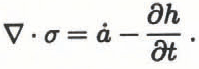
To cast this as a differential equation, one must relate the flux, σ, to the ice-surface elevation, h, through a constitutive equation. For non-Newtonian fluids, such as ice, this involves a non-linear relationship depending on the ice-surface elevation, the thickness and the surface slope.

We can, however, linearize this by absorbing all dependencies on h and all non-linearities in the surface slope into a spatially non-uniform proportionality constant k(x, y). This constitutive equation, relating ice flux to surface slope, can be expressed by

The material coefficient k(x,y) is dependent upon the form of the flow and sliding laws.

We use Glen’s flow law (Reference GlenGlen, 1955) for the component of velocity due to internal deformation of the ice, given by the following expression.

The sliding law used here is a general relationship for beds at the melting point developed by (Reference WeertmanWeertman 1957, Reference Weertman1964) and given by the following expression.

The column-averaged ice velocity for a combination of these two modes of motion is

where f is the fraction of velocity due to sliding. For existing ice sheets, f can be used as a parameter to “tune” the model. For reconstructing ice sheets from the past and for extrapolating future behavior, f can be estimated from various erosional features found in the glacial geologic record (Reference Hughes, Denton and HughesHughes, 1981).

The form of k(x,y) is obtained by combining Equations (3), (4) and (5), and substituting into Equation (2):

This shows the dependence of the material coefficient on ice density, gravity, flow-law constant and sliding-law constant (both of which are dependent on ice temperature, ice-crystal size, impurity content, etc.), ice thickness and surface gradient.

Substituting the constitutive law expression for σ from Equation (2) into continuity Equation (1) yields the following differential equation in h.

The presence of k(x, y) in the continuity equation incorporates the physics of the flow and sliding laws into the problem, since its form depends on the form of the flow and sliding law. Different treatments of the flow and sliding process change the form of k(x, y) but do not affect the method with which the problem is solved. An entirely different sliding relationship can be substituted without materially affecting the finite-element method of obtaining a solution to this equation.

The finite-element method

The finite-element method is especially well suited for solving equations such as Equation (7). The method assumes linear spatial interpolante for the solution of this differential equation, turning the problem into a set of algebraic equations which can be solved by ordinary matrix methods (Reference Becker, Carey and OdenBecker and others, 1981). The solution of these algebraic equations corresponds to the values of h at each of the nodal points defining the grid of elements used to represent the domain of the problem. Boundary conditions can either be specified ice-surface elevations or specified ice fluxes across the boundary. Material properties (such as the linearization constant, the net accumulation rate, the flow-law constant, the sliding-law constant or the fraction of the velocity due to sliding) can be specified for each node.

Due to the non-linearity in the equation represented by the linearization constant, k(x, y), we must proceed to the solution by an iterative technique. Initially, a uniform value is chosen for k(x, y) and a solution for h at each node is found. From this a new non-uniform k(x, y) is obtained from Equation (6) and a new solution for h is obtained. This process is repeated a handful of times until the values of the solution stop changing.

The mass-balance relationship

The primary input, besides the bedrock topography, is the mass balance at each node. In modeling existing ice sheets, measured values of accumulation rates can be used. However, if experiments dealing with changing climate are desired, some self-consistent mass-balance relationship that accounts for changes in the ice configuration is necessary. In the ideal, we would couple such an ice-sheet model with a global-circulation model (GCM), so that changing topography and albedo would enable us to affect the ice sheet’s own climatic conditions. With GCMs too expensive and complicated, a simpler parameterization of the ice-sheet’s effect on local climate is required for efficient experimentation. We developed a mass-balance relationship based on empirically fitting to present Antarctic accumulation rates. This relationship depends on surface elevation, surface slope, and latitude. Complementary ablation rates are based on south Greenland mass-balance data, and are appropriate for modest warming of the Antarctic climate. The climate is adjusted by varying the mean annual sea-level air temperature, T_NSL , which provides a starting point for all temperature calculations at present sea level. We understand the limitations of this very simplified model of the mass balance but feel that it is an appropriate approximation to the actual situation.

The mass-balance relationship follows Reference Fortuin and OerlemansFortuin and Oerlemans (1990) with modifications suggested by Reference Jouzel and MerlivatJouzel and Merlivat (1984) and Reference Braithwaite, Olesen and OerlemansBraithwaite and Olesen (1989).

Basically, this involves an annual average surface temperature (T_s, °C) derived from a lapse rate (A_L, °C km^-1) and modified for distance from the pole (B_L °C° lat.^-1)

From this a free atmosphere-isothermal layer temperature (T_F, K) is obtained from a standard meteorological relationship.

This temperature is used to calculate the saturation vapor pressure (E_s, mbar) from a standard meteorological relationship.

Finally, accumulation rate (A_ACC, m year^-1 ice equivalent) is obtained from a fit of accumulation rate as a function of saturation vapor pressure and surface slope (S_LOPE m km ^-1).

Ablation is modeled by calculating the number of positive degree days based on assumptions of the seasonality as a function of latitude. A seasonality factor is calculated that represents incoming solar radiation at the top of the atmosphere as a function of latitude and month. From published values (Reference SellersSellers, 1965), we obtain a latitudinal slope, QS_I (ly d^– °lat.^-1), and intercept, QS_I (ly d^-1), from which an annual mean is calculated by the following expression.

A monthly mean temperature (°C) is calculated from the mean annual temperature as a function of the difference between the annual mean and the monthly solar radiations. The proportionality constant is obtained by linear regression from 28 stations where measured monthly temperature and calculated solar radiation could be compared (Reference SchwerdtfegerSchwerdtfeger, 1984).

The annual sum of positive degree days

is used to calculate the ablation rate

where the proportionality constant applies to West Greenland ablation data (Reference Braithwaite, Olesen and OerlemansBraithwaite and Olesen, 1989). Finally, the net mass balance is the difference between these two.

Reference Fortuin and OerlemansFortuin and Oerlemans (1990) estimated parameters for the various fitting equations from available Antarctic data. We have used the Scott Polar Research Institute map (Reference Drewry and DrewryDrewry, 1983) as digitized by Budd. These data provide surface elevation, ice thickness, bedrock elevation, surface temperature, accumulation rate and balance velocity for a 20 km grid centered on the South Pole (241 × 241 grid). We differ slightly from their published values in that we have lumped together the escarpment and interior values while excluding the ice shelves. This was done to avoid a discontinuity in mass-balance values that their curves generated at the escarpment/interior boundary.

The following are the values obtained for the monthly seasonality factors. For QI_I we use 960, 1036, 1200, 825, 330, 90, 150, 600, 1200, 1020, 930 and 850°C. For QS_I, we use 0.667, 4.6, 11.667, 9.167, 3.667, 1.0, 1.0, 1.667, 6.667, 12.0, 6.333, 0.333 and -3.333°C° lat. Other fitting parameters obtained include A_L = -9.623 × 10 ^-3 °C m^-1 B = -0.5469°C° lat., C = 24.98°C, W = 0.1914 m year^-1 mbar^-1, X = 9.2228 × 10^-3 m year^-1 and Z = -7.389 × 10^-3 m year^-1, where these are all obtained by linear regression with the Scott Polar Research Institute map data.

Figure 1 shows a comparison between the fitted values generated by Equation (20) and those presented by Reference Bindschadler, Stephenson, MacAyeal and ShabtaieDrewry (1983). Major discrepancies occur mainly in the Antarctic Peninsula region and along the Amundsen Sea coast where the fit consistently underestimates the net accumulation rates.

Fig. 1.

Comparison of present Antarctic mass balance (a) with that obtained from Equation (20) (m year^-1 ice equivalent) (b).

Calibration of the model

With a mass-balance relationship such as the one described in the previous section, we can begin to look at the effects of warming or cooling the climate of Antarctica. To see the subtle effects that such changes produce, we must be confident that the other unknown parameters are defined in such a way that for the present climate we will obtain a steady-state configuration for the ice sheet which agrees well with the present configuration.

This is done in an iterative fashion by defining the spatially non-uniform linearization constant, k(x, y) from the present ice-sheet surface. But first we must define all of the 1772 nodal-point values of the flow-law constant, the sliding-law constant and the fraction of the velocity which is due to sliding (A, B and f in Equation (6)).

We do this by initially assuming a uniform value for each of these parameters, obtaining a solution, h, for several time steps, and then examining each of the nodalpoint surface-elevation values relative to the known elevation at that point. The various values of the parameters are then adjusted in a direction that will improve the fit. For example, if the surface is too high at a particular node, the flow- and sliding-law constants will be reduced and the fraction of sliding will be increased, thereby tending to reduce the surface elevation at this point and improving the fit.

This process is repeated for all the nodes collectively, until the surface attains a reasonable fit or until the parameters go outside some reasonable range of values. For instance, the sliding fraction cannot exceed 1 nor be less than 0, and the range of ice-hardness values is in some sense prescribed by the temperatures. A few dozen passes of this iterative process usually suffice to obtain a good fit, which is shown in Figure 2.

Fig. 2.

Comparison of present Antarctic surface elevation (a) with that obtained by fitting with sliding fraction, flow-law parameter and sliding-law parameter (m above present sea level) (b).

Figure 3 shows the distribution of the sliding fraction that was obtained in this fitting process. Note the almost complete dominance of flow throughout the interior of the ice sheet. Sliding only occurs in localized regions around the margin of the ice sheet and in regions known to be associated with ice streams, such as the ice streams along the Siple Coast, the ice streams that feed the Amery Ice Shelf and Pine Island and Thwaites Glaciers, as well as some of the major outlet ice streams that flow through the Transantarctic Mountains. In addition, there is a large region of sliding surrounding and to the east of the Filchner-Ronne Ice Shelf. Qualitatively, this agrees well with where sliding might be expected to occur.

Fig. 3.

Distribution of sliding fraction obtained in the fitting process.

Figure 4 shows the distribution of the flow-law parameter that was obtained in this fitting process. The bulk of the values in regions where flow dominates are between 2.5 and 3.5 bar year^1/3, with an average value of 2.97 for the 850 nodes (out of 1316 ice-covered nodes) with sliding fraction less than or equal to 0.1. In addition, note that the higher values (i.e. harder ice) tend to occur further from the coast where the ice is in general colder. The regions of soft ice corresponding to small flow-parameter values occur mainly in areas where sliding dominates so these do not affect the ice-sheet surface elevation.

Fig. 4.

Distribution of flow-law parameter obtained in the fitting process (bar year^1/3).

The distribution of the sliding parameter is similar to the distribution of the flow-law parameter, again with extreme values occurring mainly in regions where flow dominates. Because of the limited areas where sliding dominates this is not shown. In regions where the sliding dominates (466 nodes out of 1316 for sliding fraction greater than 0.1), the average value of the sliding parameter is 0.0277 bar year^1/2. In regions where the sliding fraction is particularly high (greater than 0.9), the sliding parameter is lower, with an average value of 0.0129 for 217 nodes. This could reflect the fact that regions of high sliding fraction are controled by some mechanism that leads to greater decoupling of the bed, such as deformable sediments.

Variation of the sea-level mean annual air temperature

To see the effect of variation of the climate on the volume and areal extent of the Antarctic ice sheet, a number of experiments were performed for various values of T_NSL. In each case, the value of the mean annual sea-level temperature was adjusted, and the model allowed to run for 9000 years, a time period that approximated equilibrium conditions. In this time period, the major adjustments in the shape and response of the ice sheets have occurred, although there is still an adjustment remaining as the high-elevation, low accumulation-rate parts of the ice sheet equilibrate. These further adjustments are small and, since the climate system rarely remains in the same state for much longer than 10 000 years, this response was not considered to be important. Shown in Table 1 are flotation volume, total volume, areal extent, average thickness and maximum surface elevation for various values of T_NSL. The flotation volume differs from the total volume in that it is the part of the ice sheet that would contribute to sea-level rise if the entire ice sheet were melted. This part of the column does not contribute to the rise in sea level and hence is not included in the volume calculation.

Table 1.

Flotation volume, total volume, area, average thickness and dome elevation as a function Of T_NSL

Table 2 shows the same results normalized with respect to the present configuration, which corresponds to a value for T_NSL of -14°C. Figure 5 shows the same results in a graphical form. Note that the maximum increase in volume occurs for a temperature increase of 6 deg, and that both average thickness and dome elevation continue to increase as the temperature warms. This is due to the increasing accumulation rates at high elevations, a consequence of the increasing saturation vapor pressure as the climate warms. While ablation rates also increase, their effect is primarily at lower elevations which results in a decrease in the areal extent of the ice sheet as the climate warms.

Fig. 5.

Flotation volume, total volume, area, average thickness and dome elevation as a function of T_NSL, normalized to the configuration for present conditions at -14°C.

Table 2.

Ratios of flotation volume, total volume, area, average thickness and dome elevation to the configuration for -14°C as a function of T_NSL

Extreme configurations

Time-dependent experiments

The experiments thus far have dealt with equilibrium situations that are attained by applying a sudden change to an initial condition and allowing the system to respond. As the rate of change of the system decreases, the system approaches an equilibrium state. In reality the ice sheet will rarely attain such an equilibrium configuration, since before that state is attained the driving mechanism will have changed, either abruptly or in some continuous fashion.

To demonstrate the response of the Antarctic ice sheet to a smoothly varying driving force, a smooth sinusoidal variation of the mean annual sea-level temperature, T_NSL, is applied over a time span of 20 000 years. The cycle begins with T_NSL at its current value of -14°C, and the ice sheet in its equilibrated “best-fit” configuration. Over 20 000 years, the temperature is warmed to -8°C, then cooled down to -20° C, and then warmed back up to -14°C. This driving force is shown in Figure 10 by the dashed line. The response of the ice sheet is to change both volume and areal extent. The total volume is shown in Figure 10 by the solid line. Vertical lines indicate both peaks and valleys of the two curves. The volume response of the ice sheet lags the driving-force temperature by approximately 2700 years, as the volume changes just under 10% of its total volume. There is some indication that this lag depends slightly on the amplitude of the driving-force variations, as a similar simulation with a smaller temperature swing showed a lag of just over 2000 years.

Fig. 10.

Total volume versus time shown with the T_NSL curve to show the lag in the ice sheet’s response. The dashed line is the driving parameter and the solid line is the system’s response.