Sensor’s presentation

The sensor (Fig. 1) consists of a microstrip line (operating in transmission mode) loaded symmetrically by two rectangular SRRs printed on a 1.524 $mm$ thick Arlon 25N substrate ( $\epsilon_r$ = 3.32; $\tan\delta$ = 0.0025) with 17  $\mu m$ thick copper metallization. The width of the microstrip line $W$ is dimensioned to have a 50  $\Omega$ characteristic impedance ( $W$ = 3.8  $mm$). The detection area of each SRR corresponds to the aperture of the metallic ring. In order to take advantage of the strong electric field amplitude within the substrate, the gaps in both resonators have been carved [Reference Pichereau, Fritiss, Takhedmit, Poulichet, Lanquetin, Français and Richalot14]. These cavities, having each one a small volume of around 23  $\mu l$ per hole, can then be filled (using a syringe) with the liquids under test. The width of each SRR $W_{Srr}$, its length $L_{Srr}$, the distance between each SRR and the microstripline $d$, the gap $g$ and the SRR line width $c$ are, respectively, of 22  $mm$, 20  $mm$, 1  $mm$, 3  $mm$, and 2  $mm$. The unloaded resonant frequency is 1.35 GHz.

While modeling the rectangular SRR as a combination of an inductance, a resistor and a capacitor, the equivalent circuit representation of the differential sensor is shown in Fig. 1 (right) [Reference Ebrahimi, Scott and Ghorbani6].

Figure 1.

Presentation of sensor consisting of two SRRs excited by a microstrip line: Photograph of the fabricated sensor (left), a sketch indicating the geometrical parameters (middle), and an equivalent circuit model of the sensor consisting of two RLC-circuits (related to both SRRs) inductively coupled to the transmission line via $M$, with a mutual inductance between resonators $M_b$ (right).

Figure 1 Long description

The image consists of three parts. On the left, there is a photograph of the fabricated sensor, which includes two rectangular split-ring resonators symmetrically loaded onto a microstrip line. The resonators are printed on a substrate and the photograph shows the physical setup with connectors on either side of the microstrip line. In the middle, a sketch illustrates the geometrical parameters of the sensor. The sketch shows the microstrip line running horizontally, with two split-ring resonators positioned vertically above and below it. The resonators are labeled with dimensions: the width of the microstrip line is marked as W, the width of each SRR as W subscript SRR, the length of each SRR as L subscript SRR, the distance between each SRR and the microstrip line as d, the gap in the resonators as g and the SRR line width as c. On the right, an equivalent circuit model is depicted, consisting of two RLC circuits related to the SRRs. These circuits are inductively coupled to the transmission line via mutual inductance labeled M, with additional mutual inductance between the resonators labeled M subscript b. The circuit includes capacitors labeled C subscript 1 and C subscript 2, inductors labeled L and resistors labeled R subscript 1 and R subscript 2. Arrows indicate the direction of coupling between the components.

The access microstrip line is modeled by an inductance $L_{m}$, and both SRRs are coupled with the microstrip line through the mutual inductance $M$, whereas $M_b$ represents the mutual coupling between both resonators. When both sensors are symmetrically loaded (using the same sample in both gaps), $C_{1}$ is equal to $C_{2}$ and $R_{1}$ is equal to $R_{2}$. When the material under test is placed in the gap of the SRR, the equivalent capacitance associated with the gap is modified, which subsequently leads to a shift in the resonant frequency [Reference Withayachumnankul, Jaruwongrungsee, Tuantranont, Fumeaux and Abbott4]. Using two SRRs permits to achieve differential measurements when both SRRs are loaded asymmetrically. In particular, one SRR can be used as a reference if it is loaded by a sample of known properties. This differential approach reduces the impact of the environment on the measurement results [Reference Mohammadi, Nadaraja, Luckasavitch, Jain, Roberts and Zarifi8].

Fabrication and methods for liquid mixing

The sensor (on the left of Fig. 1) has been fabricated in the ESYCOM laboratory using the LPKF Protomat S100 prototyping machine, based on mechanical etching. Water–ethanol solutions with different concentrations were produced in 50  $ml$ flasks using 0.2  $ml$ precision pipettes. To measure their dielectric properties, the commercial Keysight 85070E Dielectric Probe Kit [Reference Technologies15] has been used, and the obtained values are compared here with the ones obtained using Birchak’s theoretical mixing law [Reference Birchak, Gardner, Hipp and Victor16, Reference Sihvola17] over the frequency band from 1 GHz to 1.5 GHz. Birchak’s law is used to define the parameters of the Debye model (Eq. 1) that are the low-frequency (Eq. 2) and the high-frequency (Eq. 3) permittivities of the different liquid mixtures according to the ratio $\alpha$ of a first liquid volume to the total bi-liquid mixture volume. The relaxation frequency (Eq. 4) is calculated following [Reference Yang, Yang, Huang, Shang and Jia18]. Thus, the frequency variation of the complex relative permittivity of each mixture is obtained.

(1)\begin{equation} \epsilon^*_{r(mix)} = \epsilon_{\infty(mix)} +\frac{(\epsilon_{s(mix)} -\epsilon_{\infty(mix)})}{1+j \frac{f}{f_{rel(mix)}}} \end{equation}

(2)\begin{equation} \epsilon_{s(mix)} = \left[\alpha \sqrt{\epsilon_{s(1)}} + (1-\alpha) \sqrt{\epsilon_{s(2)}} \right]^2 \end{equation}

(3)\begin{equation} \epsilon_{\infty(mix)} = \left[\alpha \sqrt{\epsilon_{\infty(1)}} + (1-\alpha) \sqrt{\epsilon_{\infty(2)}} \right]^2 \end{equation}

(4)\begin{equation} f_{rel(mix)} = \exp\left[\alpha\ln(f_{rel(1)}) + (1-\alpha) \ln(f_{rel(2)}) \right]\,. \end{equation}

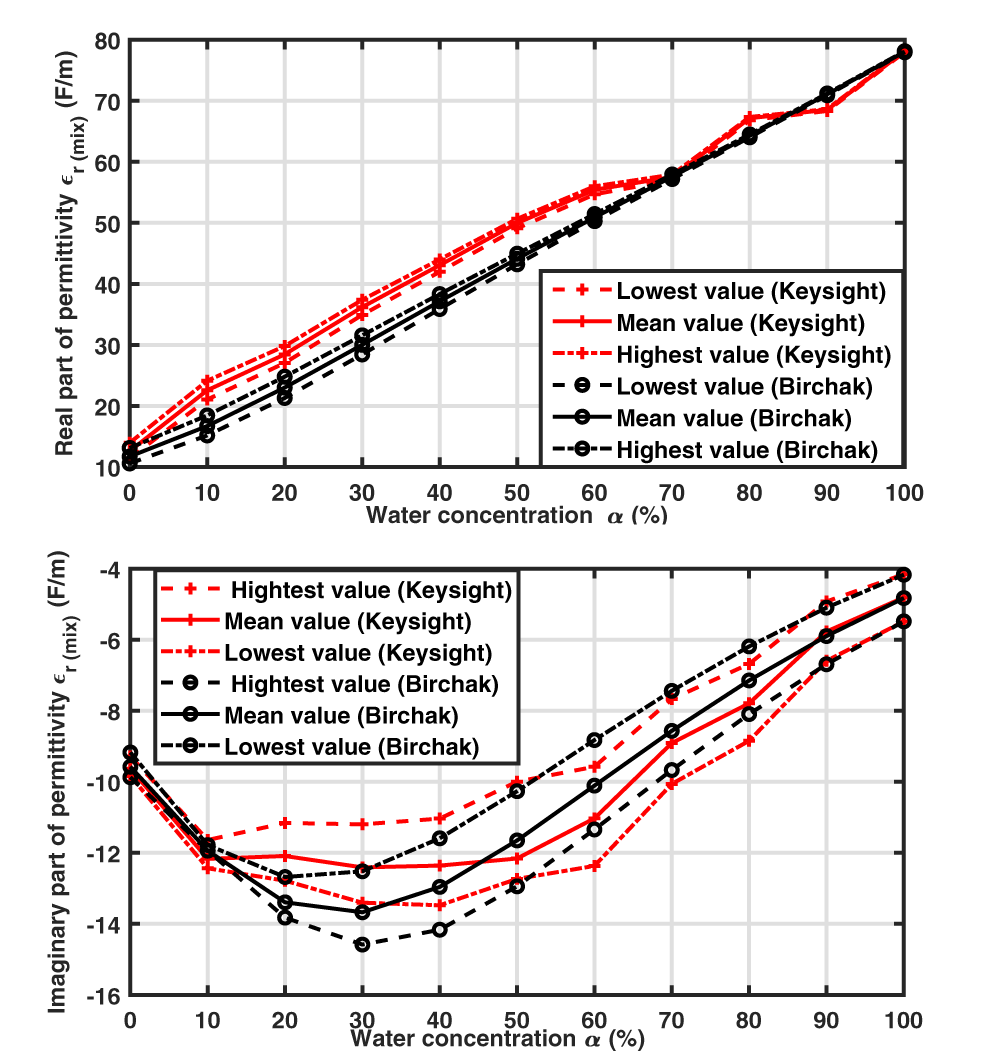
Note that $\epsilon_{s(1)}$, $\epsilon_{\infty(1)}$, and $f_{rel(1)}$ are, respectively, associated with the low-frequency permittivity, high-frequency permittivity and relaxation frequency of the first liquid in the mixture, while $\epsilon_{s(2)}$, $\epsilon_{\infty(2)}$, and $f_{rel(2)}$ are related to the second liquid in the mixture. The frequency is denoted $f$. In our case, the two liquids of interest are water and ethanol, whose Debye’s parameters are depicted in Table 1. Figure 2 depicts the mean, minimal, and maximal values, over the 1-1.5 GHz frequency band, of the permittivity’s real and imaginary parts of the measured liquid samples that are obtained using Birchak’s formulae and measured using the Keysight probe. The measured real part (polarization effect) is consistent with the mixing law, whereas the imaginary part (loss effect) follows the same pattern but with fluctuations around the expected values. Note that the imaginary part of the permittivity is negative due to the chosen time dependence as $e^{j\omega t}$. The various errors encountered can be associated with the uncertainties during the sample preparation process along with the Keysight probe resolution of $\pm 5\%$ for the real and imaginary parts [Reference Technologies15].

Figure 2.

Real and imaginary parts of relative permittivities extracted by the Keysight probe compared to the ones given by the Birchak mixing law in the 1–1.5 GHz frequency band: mean, minimal, and maximal values over this frequency band for each water percentage of the mixtures.

Figure 2 Long description

Real part of permittivity epsilon r subscript mix (F slash m) The x-axis is labeled Water concentration alpha (percent), ranging from 0 to 100 in increments of 10. The y-axis is labeled Real part of permittivity epsilon r subscript mix (F slash m), ranging from 10 to 80 in increments of 10. The legend lists six series: Lowest value (Keysight), Mean value (Keysight), Highest value (Keysight), Lowest value (Birchak), Mean value (Birchak), Highest value (Birchak). Keysight lowest value: 0 percent about 12; 10 percent about 20; 20 percent about 26; 30 percent about 33; 40 percent about 40; 50 percent about 46; 60 percent about 52; 70 percent about 58; 80 percent about 66; 90 percent about 69; 100 percent about 78. Keysight mean value: 0 percent about 12; 10 percent about 21; 20 percent about 27; 30 percent about 34; 40 percent about 41; 50 percent about 47; 60 percent about 53; 70 percent about 58; 80 percent about 67; 90 percent about 69; 100 percent about 78. Keysight highest value: 0 percent about 13; 10 percent about 23; 20 percent about 29; 30 percent about 36; 40 percent about 44; 50 percent about 50; 60 percent about 56; 70 percent about 59; 80 percent about 68; 90 percent about 69; 100 percent about 78. Birchak lowest value: 0 percent about 11; 10 percent about 16; 20 percent about 22; 30 percent about 29; 40 percent about 36; 50 percent about 43; 60 percent about 50; 70 percent about 58; 80 percent about 64; 90 percent about 71; 100 percent about 78. Birchak mean value: 0 percent about 11; 10 percent about 17; 20 percent about 23; 30 percent about 30; 40 percent about 37; 50 percent about 44; 60 percent about 51; 70 percent about 58; 80 percent about 65; 90 percent about 71; 100 percent about 78. Birchak highest value: 0 percent about 12; 10 percent about 18; 20 percent about 24; 30 percent about 31; 40 percent about 38; 50 percent about 45; 60 percent about 52; 70 percent about 58; 80 percent about 66; 90 percent about 71; 100 percent about 78. Imaginary part of permittivity epsilon r subscript mix (F slash m) The x-axis is labeled Water concentration alpha (percent), ranging from 0 to 100 in increments of 10. The y-axis is labeled Imaginary part of permittivity epsilon r subscript mix (F slash m), ranging from minus 16 to minus 4 in increments of 2. The legend lists six series: Highest value (Keysight), Mean value (Keysight), Lowest value (Keysight), Highest value (Birchak), Mean value (Birchak), Lowest value (Birchak). Keysight highest value: 0 percent about minus 9.5; 10 percent about minus 12.0; 20 percent about minus 11.0; 30 percent about minus 11.0; 40 percent about minus 10.8; 50 percent about minus 10.0; 60 percent about minus 9.5; 70 percent about minus 7.5; 80 percent about minus 6.0; 90 percent about minus 4.8; 100 percent about minus 4.0. Keysight mean value: 0 percent about minus 9.8; 10 percent about minus 12.0; 20 percent about minus 12.0; 30 percent about minus 13.0; 40 percent about minus 13.0; 50 percent about minus 12.0; 60 percent about minus 11.0; 70 percent about minus 8.5; 80 percent about minus 7.0; 90 percent about minus 5.8; 100 percent about minus 4.8. Keysight lowest value: 0 percent about minus 10.0; 10 percent about minus 12.2; 20 percent about minus 13.0; 30 percent about minus 13.5; 40 percent about minus 13.5; 50 percent about minus 13.0; 60 percent about minus 12.5; 70 percent about minus 10.0; 80 percent about minus 8.8; 90 percent about minus 6.5; 100 percent about minus 5.5. Birchak highest value: 0 percent about minus 9.2; 10 percent about minus 12.0; 20 percent about minus 12.8; 30 percent about minus 12.5; 40 percent about minus 11.5; 50 percent about minus 10.0; 60 percent about minus 8.8; 70 percent about minus 7.2; 80 percent about minus 6.0; 90 percent about minus 4.8; 100 percent about minus 4.0. Birchak mean value: 0 percent about minus 9.5; 10 percent about minus 12.0; 20 percent about minus 13.2; 30 percent about minus 13.5; 40 percent about minus 13.0; 50 percent about minus 11.5; 60 percent about minus 10.0; 70 percent about minus 8.5; 80 percent about minus 7.5; 90 percent about minus 5.8; 100 percent about minus 4.5. Birchak lowest value: 0 percent about minus 9.8; 10 percent about minus 12.2; 20 percent about minus 13.8; 30 percent about minus 14.5; 40 percent about minus 14.0; 50 percent about minus 13.0; 60 percent about minus 11.2; 70 percent about minus 9.5; 80 percent about minus 8.0; 90 percent about minus 6.5; 100 percent about minus 5.2.

Table 1.

Material parameters of the Debye model at 25 $^{\circ}$C

Table 1 Long description

The table lists Debye-model dielectric parameters for two liquids at room temperature. For each material, it reports static permittivity, high-frequency permittivity, and relaxation frequency in gigahertz. Water has a static permittivity of 78.36, compared with 24.43 for ethanol, indicating a much stronger low-frequency dielectric response. Their high-frequency permittivity values are closer, at 5.2 for water and 4.5 for ethanol. Water’s relaxation frequency is 19.24 gigahertz, far higher than ethanol’s 0.96 gigahertz, meaning water’s polarization response shifts at much higher frequencies. Values are specific to the stated temperature and the Debye-model fit, so they may differ under other conditions or with different modeling assumptions.

Experimental conditions and measurement results

Transmission measurements between both SMA accesses are performed using a Rohde & Schwarz ZNB20 Vector Network Analyzer (VNA) with 2001 frequency points between 1 and 1.5 GHz. To carry out differential measurements, the cavity of one resonator is loaded with a reference sample that remains unchanged during the series of measurements, while the cavity of the second resonator is successively loaded with deionized water–ethanol solutions with different concentrations.

Three different reference choices have been considered: air (empty resonator), ethanol, and deionized water (Fig. 3). The measurement campaigns with the different references were not all carried out at the same time. Since the reproducibility of measurements with the sensor is not guaranteed, a frequency shift in the reference is possible from one measurement campaign to another, particularly because the sample volume is not controlled or monitored. However, this does not affect the resonance extraction method presented in this paper.

Figure 3.

Measurement campaigns with different references were not carried out at the same time. Since the reproducibility of measurements with the sensor cannot be guaranteed, a frequency shift of the reference is possible from one measurement campaign to another, particularly because the sample volume is not controlled or monitored. Transmission coefficient magnitude for a reference sample of (a) air (top), (b) ethanol (middle), or (c) water (bottom) in one SRR, whereas the second SRR is loaded with a mixture of deionized water and ethanol of varying concentration, including the pure ethanol and water cases: legend “water mWnE” means water as reference, m $\%$ of water and n $\%$ of ethanol.

Figure 3 Long description

The image A showing a line graph with the y-axis labeled Transmission coefficient magnitude (decibel) and the x-axis labeled Frequency (gigahertz). The x-axis ranges from 1 to 1.5 with tick marks at 1, 1.05, 1.1, 1.15, 1.2, 1.25, 1.3, 1.35, 1.4, 1.45 and 1.5. The y-axis ranges from 0 to minus 6 with tick marks at 0, minus 1, minus 2, minus 3, minus 4, minus 5 and minus 6. Multiple colored curves are plotted. Each curve stays near 0 at the left, then drops into a narrow dip between about 1.1 and 1.2, then returns toward 0. One curve also shows a deeper dip near about 1.33 reaching close to minus 6. The image B showing a line graph with the y-axis labeled Transmission coefficient magnitude (decibel) and the x-axis labeled Frequency (gigahertz). The x-axis ranges from 1 to 1.5 with tick marks at 1, 1.05, 1.1, 1.15, 1.2, 1.25, 1.3, 1.35, 1.4, 1.45 and 1.5. The y-axis ranges from 0 to minus 4 with tick marks at 0, minus 1, minus 2, minus 3 and minus 4. Multiple colored curves are plotted. The curves show dips clustered between about 1.1 and 1.2, with minima ranging roughly from about minus 2 to near minus 4, then rising back toward 0 by about 1.3 to 1.5. The image C showing a line graph with the y-axis labeled Transmission coefficient magnitude (decibel) and the x-axis labeled Frequency (gigahertz). The x-axis ranges from 1 to 1.5 with tick marks at 1, 1.05, 1.1, 1.15, 1.2, 1.25, 1.3, 1.35, 1.4, 1.45 and 1.5. The y-axis ranges from 0 to minus 4 with tick marks at 0, minus 1, minus 2, minus 3 and minus 4. A legend lists ten series: 0W100E, 10W90E, 20W80E, 30W70E, 40W60E, 50W50E, 60W40E, 70W30E, 80W20E, 90W10E. Multiple colored curves are plotted. The curves show a sharp dip near about 1.1 to 1.15, with minima around minus 3 to near minus 4, followed by several broader dips between about 1.2 and 1.35 where different curves reach minima around minus 1 to about minus 3, then all rise toward 0 approaching 1.5.

Different behaviors are observed depending on the reference choice. With air as reference (Fig. 3a), two separated resonance peaks are observed for every mixture concentration, with a fixed resonance at 1.29 GHz corresponding to the reference (unloaded resonator), whereas the second resonance frequency decreases when the water concentration increases in agreement with the relative permittivity real part increase (Fig. 2). The highest difference between both resonance frequencies, obtained in the air/water loading case, is 174 MHz. When ethanol is used as a reference (Fig. 3b), two resonance peaks can still be distinguished when the second SRR is loaded with water; this loading case corresponds to the highest resonance frequency difference between both resonances, which is 98 MHz. This lower value in regard to the previous reference case (air) is explained by a smaller permittivity difference between both loading samples. When the ethanol concentration of the mixture increases, in particular for an ethanol concentration above 50 $\%$, it becomes difficult to distinguish both resonances due to a strong overlap between resonance peaks, so that there is no stable reference peak in this case. With the third reference choice (deionized water) (Fig. 3c), distinct resonance peaks are obtained for the lowest water concentrations of the mixtures, whereas resonance overlapping occurs when the mixture composition becomes closer to that of the reference sample.

In order to avoid this resonance overlap occurring in differential structures, some authors have proposed an asymmetric structure with a reference resonator associated with a resonance frequency outside the resonance frequency band of the sensing resonator [Reference Vélez, Muñoz-Enano, Grenier, Mata-Contreras, Dubuc and Martín9]. In this paper, a symmetric structure has been chosen to permit the use of a reference liquid sample of the same type as the sample under test. Thus, the reference resonance is shifted in a very close way to the sample under test ensuring a weaker sensitivity to environmental effects than asymmetric sensors. The flexibility in the reference sample choice is an advantage of this differential structure as it can be adapted to the samples under test and the application objectives. The choice of a reference sample of permittivity far from the one of the sample under test permits a simple comparison of both resonance frequencies and widths, as both resonance peaks are separated; however, choosing a reference that fulfills this condition is difficult with samples of unknown properties. Besides, the choice of a reference sample similar to the sample under test can also be relevant for detecting a slight discrepancy between their compositions. As an example, a difference is observed in Fig. 3(c) between the transmission parameters measured with a mixture containing 90 $\%$ of water and the one related to the very similar mixture containing 80 $\%$ of water and 20 $\%$ of ethanol, with a variation of the minimal transmission value, even though the two peaks are not distinguishable to the naked eye. In this case, the determination of the sensor resonance properties is not possible using classical resonance analysis techniques.

In the following analyses, the measurement results obtained with deionized water chosen as the reference material are depicted. Figure 3(c) depicts the magnitude variation of the measured transmission coefficients in the different asymmetrical loading conditions. One observes for all curves the presence of a magnitude peak around 1.18 GHz, which is related to the resonance of the SRR loaded by water, and a second resonance, also associated with a magnitude peak, whose position and width vary according to the mixture used. As expected, it is obvious that the highest difference between both resonance frequencies is obtained with the ethanol sample, whereas this difference decreases when the percentage of water within the mixture increases. The positions and widths of both peaks can be clearly distinguished as a function of mixture concentration in many cases. However, when the composition of both samples is close, as with the mixture composed of $90\%$ of water and $10\%$ of ethanol, the two resonances form a single peak so that it is difficult to distinguish their widths or central frequencies. This is why a post-processing method is proposed in the following; the complex value of the transmission coefficient will be exploited since the magnitude alone is not enough to extract the resonance properties.

Resonance parameters extraction method in resonance overlapping condition

The resonance of each SRR, associated with its RLC-equivalent model (on the right of Fig. 1), is modeled with an equation to a term having a frequency variation of the form:

(5)\begin{equation} S_r = \frac{A}{1+j\,2 \pi f R C - L C(2\pi f)^2} \end{equation}

with a numerator $A$ slowly varying around the resonance frequency, leading to a resonance frequency of $f_r = \frac{1}{2\pi \sqrt{LC}}$ and a quality factor $Q = \frac{f_r}{\Gamma} = \frac{1}{2\pi f_r RC}$, where $\Gamma$ is the resonance bandwidth [Reference Alahnomi, Zakaria, Ruslan, Rashid and Bahar1]. As a consequence, the contribution of the SRR resonance to the transmission coefficient can be written as $S_r = (A f_r^2)/(f_r^2 - f^2 + jf\Gamma)$. Close to the resonance frequency, approximations can be performed ( $f_r^2 - f^2 + jf\Gamma \approx 2f_r.(f_r - f) + jf_r\Gamma$) to simplify this expression and obtain the Lorentzian:

(6)\begin{equation} S_r = \frac{-A \frac{f_r}{2}}{f-(f_r+j\Gamma /2)}\,. \end{equation}

Therefore, to extract the properties of both resonances, even when their proximity induces an overlapping that makes them difficult to distinguish, the measured complex-valued transmission amplitude ${S}_{21}$ is fitted by representing the two resonances as Lorentzians with a complex linear background:

(7)\begin{equation} S_{21} = \frac{a_1}{f - f_{r,1}-jf_{i,1}} + \frac{a_2}{f-f_{r,2}-jf_{i,2}} + c_1 f + c_0\,, \end{equation}

where $a_i$ are the complex amplitudes, $f_{r,i}$ the eigenfrequencies, and $\Gamma_i=2f_{i}$ the resonance widths ( $i=1,2$). $c_1 \in \mathbb{C}$ are the slope of the linear background and $c_0\in \mathbb{C}$ a constant. This fitting, however, requires first removing the frequency slope of the phase of $S_{21}$ related to the propagation phenomenon along the microstrip line. This slope $b$ is extracted from the measured argument, and the original transmission coefficient $S_{21}$ is then modified through the multiplication:

(8)\begin{equation} \hat{S}_{21} = S_{21} \textrm{e}^{-j (b f+\varphi_0)}\,, \end{equation}

where $\varphi_0$ is chosen to cancel out the phase outside the resonances. Figure 4 illustrates this operation, which consists of removing the global phase slope on the measurement results obtained with a mixture containing $80\%$ of water and $20\%$ of ethanol, as well as with a mixture of $90\%$ of water and $10\%$ of ethanol.

Figure 4.

Measured phase of $S_{21}$ with one SRR loaded by deionized water and the other one by a mixture of 80 $\%$ water and 20 $\%$ ethanol: initial values (in black), phase after removing the phase slope (as an initial step before performing the curve fitting), and fitted phase using the expansion on Lorentzians. Inset: the corresponding curves are presented for the 90W10E mixture.

Figure 4 Long description

Transmission coefficient phase (rad) The x-axis is labeled Frequency (GHz), ranging from 1.0 to 1.5 with tick marks at 1.0, 1.05, 1.1, 1.15, 1.2, 1.25, 1.3, 1.35, 1.4, 1.45 and 1.5. The y-axis is labeled Transmission coefficient phase (rad). A legend lists four series: After slope removing, Reconstructed signal, Initial phase and Resonant frequencies. Three overlaid curves run across the full frequency range. A dashed line slopes downward from left to right. Two vertical dashed lines appear near 1.2 GHz, labeled as resonant frequencies. Around these vertical markers, the main phase curves show a sharp step-like change. An inset plot in the upper right shows the same variables over a narrower frequency range, with the x-axis labeled Frequency (GHz) and tick labels from about 1.05 to 1.4.

After this global phase slope removal, the transmission coefficient $\hat{S}_{ab}$ is fitted to the expression (7). As an example, Fig. 5 (respectively Fig. 4) shows the magnitude (resp. phase) of the measured transmission coefficient of a mixture composed of $80\%$ of water and $20\%$ of ethanol along with the fitting curve. To exemplify the modal overlapping effect, a very good agreement between the initial and fitted curves is observed (Inset Fig. 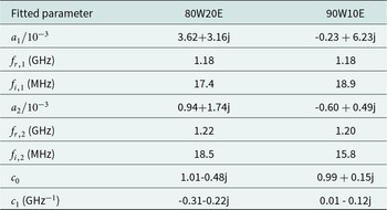5 case $90\%$ water and $10\%$ ethanol). The parameters extracted in this case using the fitting process are listed in Table 2 (for a frequency expressed in GHz in eq. (7)). Both resonance frequencies, at 1.181 and 1.219 GHz are indicated in Figs. 4 and 5. The dominant contribution of the first resonance, as indicated by a deeper peak in Fig. 5, results in a coefficient $a_1$ of magnitude 2.4 times higher than $a_2$. To amplify the modal overlapping effect, a mixture containing $90\%$ of water and $10\%$ of ethanol is presented in Figs. 5 and 4. In this case, the variation of the relative permittivities at 1.35 GHz between the reference sample (water) and the liquid under test (mixture with 90 $\%$ of water) is of 7. The extracted parameters in Table 2 show the stability of the first resonance peak and a decrease of the second one, leading to a difference between both resonance frequencies of the same order of magnitude as the resonance widths. In spite of a strong modal overlap and an important imbalance between amplitudes, the agreement between initial and reconstructed curves is still excellent.

Figure 5.

Initial and reconstructed transmission coefficient magnitude in the case of $80\%$ water and $20\%$ ethanol with water as reference. In the inset, the same curves are presented for the 90W10E mixture.

Figure 5 Long description

Transmission coefficient magnitude (dB) A line graph with two plotted curves and a legend. The x-axis is labeled Frequency (GHz), with tick labels from 1.0 to 1.5. The y-axis is labeled Transmission coefficient magnitude (dB), with tick labels from 0 to minus 3. The legend shows three entries: After slope removing (solid line), Reconstructed signal (dashed line) and Resonant frequencies (vertical dotted lines). Both curves start near 0 dB at 1.0 GHz, then decrease to a minimum near 1.18 GHz at about minus 3 dB, then rise toward about minus 1 dB by about 1.22 GHz and continue rising toward near 0 dB by about 1.5 GHz. Two vertical dotted lines are drawn near 1.18 GHz and near 1.22 GHz. An inset plot at the right shows the same axes labels. The inset x-axis shows tick labels from 1.1 to 1.35. The inset y-axis shows tick labels from 0 to minus 3. The inset curves show the same notch shape, with the minimum near 1.18 GHz at about minus 3 dB and a smaller dip near 1.22 GHz around about minus 1 dB. The same two vertical dotted lines appear in the inset near 1.18 GHz and near 1.22 GHz.

Table 2.

Fitted parameters for two different water–ethanol mixtures with water as reference

Table 2 Long description

The table lists fitted complex amplitudes, two resonance frequencies, two damping terms, and two background coefficients for two water ethanol mixtures: 80 percent water 20 percent ethanol and 90 percent water 10 percent ethanol, with water used as the reference. For the first resonance, both mixtures have the same resonance frequency of 1.18 gigahertz, while the damping is 17.4 megahertz for the 80 percent water mix and 18.9 megahertz for the 90 percent water mix. The first complex amplitude is larger for the 80 percent water mix, with real part 3.62 and imaginary part 3.16, compared with real part negative 0.23 and imaginary part 6.23 for the 90 percent water mix. For the second resonance, the 80 percent water mix has a slightly higher resonance frequency at 1.22 gigahertz versus 1.20 gigahertz for the 90 percent water mix, and higher damping at 18.5 megahertz versus 15.8 megahertz. The second complex amplitude is 0.94 plus 1.74 imaginary for the 80 percent water mix, and negative 0.60 plus 0.49 imaginary for the 90 percent water mix. Background terms differ: the constant term is 1.01 minus 0.48 imaginary for the 80 percent water mix and 0.99 plus 0.15 imaginary for the 90 percent water mix, while the linear term is negative in both parts for the 80 percent water mix and near zero real with negative imaginary for the 90 percent water mix. Because these are fitted parameters, differences reflect the chosen model and fitting procedure rather than direct measurements of a single physical quantity.

Extracted resonance parameters

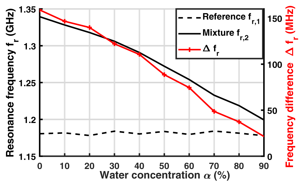
The application of this presented fitting post-process has permitted the extraction of the resonance properties for all tested mixtures, even in the case ( $90\%$ of water, $10\%$ of ethanol) where only one resonance peak is clearly visible in the transmission coefficient magnitude (Fig. 3). The variation of both resonance frequencies $f_{r,1}$ and $f_{r,2}$ is presented in Fig. 6 versus the water concentration of the tested mixture. The lowest resonance frequency $f_{r,1}$, mainly associated with the resonator loaded with water chosen as the reference when the resonances are well separated, remains stable, whereas $f_{r,2}$, associated with the liquid under test, decreases when the concentration of water increases. This is explained by the increase in the sample permittivity real part with water concentration (Fig. 2), which results in the increase of the capacitive effect $C_2$ and, as a consequence, in the decrease of the resonance frequency $f_{r,2} = 1/(2\pi \sqrt{LC_2})$. 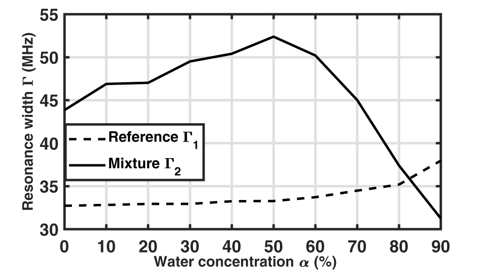The difference between both resonance frequencies $\Delta f_r$ is plotted in Fig. 6 (right vertical axis). This difference decreases almost linearly from 160 MHz to 20 MHz as the water concentration increases, in accordance with the real part of the mixture’s permittivity. It becomes lower than the resonance width $\Gamma_{2}$ for a water concentration of 90 $\%$ (Fig. 7), explaining the difficulty in distinguishing both resonances.

Figure 6.

Variation of both extracted resonant frequencies, related to the reference material (water) and to the mixture, and difference between them. Values extracted from measured transmission coefficients through the curve fitting.

Figure 6 Long description

Resonance frequency f subscript r (gigahertz) A line graph with two vertical scales. The horizontal axis is labeled Water concentration alpha (percent), with ticks at 0, 10, 20, 30, 40, 50, 60, 70, 80, 90. The left vertical axis is labeled Resonance frequency f subscript r (gigahertz), ranging from 1.15 to 1.35 with ticks at 1.15, 1.20, 1.25, 1.30, 1.35. The right vertical axis is labeled Frequency difference delta f subscript r (megahertz), ranging from 0 to 150 with ticks at 0, 50, 100, 150. Legend entries: Reference f subscript r,1 shown as a dashed line. Mixture f subscript r,2 shown as a solid line. delta f subscript r shown as a line with plus markers. Reference f subscript r,1 (dashed line, left axis): values stay near 1.18 across all water concentrations, with small changes around 0 to 90 percent. Mixture f subscript r,2 (solid line, left axis): starts near 1.34 at 0 percent, then decreases with water concentration, passing near 1.30 at 30 percent, near 1.27 at 50 percent, near 1.23 at 70 percent and reaching about 1.20 at 90 percent. delta f subscript r (plus markers, right axis): starts near 160 at 0 percent, then decreases with water concentration, near 150 at 10 percent, near 145 at 20 percent, near 130 at 30 percent, near 115 at 40 percent, near 90 at 50 percent, near 75 at 60 percent, near 50 at 70 percent, near 40 at 80 percent and near 25 at 90 percent.

Figure 7.

Resonance widths $\Gamma_1 = 2f_{i,1}$ and $\Gamma_2 = 2f_{i,2}$ as a function of the mixture water concentration.

Figure 7 Long description

Resonance width Gamma (Megahertz) Water concentration alpha (percent) Legend: Reference Gamma subscript 1 Mixture Gamma subscript 2 Horizontal axis label: Water concentration alpha (percent) Horizontal axis range: 0 to 90 Horizontal axis tick labels: 0, 10, 20, 30, 40, 50, 60, 70, 80, 90 Vertical axis label: Resonance width Gamma (Megahertz) Vertical axis range: 30 to 55 Vertical axis tick labels: 30, 35, 40, 45, 50, 55 Reference Gamma subscript 1 coordinate pairs: (0, 33), (10, 33), (20, 33), (30, 33), (40, 33.5), (50, 33.5), (60, 34), (70, 34.5), (80, 35), (90, 38) Mixture Gamma subscript 2 coordinate pairs: (0, 44), (10, 47), (20, 47), (30, 49.5), (40, 50.5), (50, 52.5), (60, 50.5), (70, 45), (80, 37.5), (90, 31.5).

The resonance width $\Gamma_{1}$ associated with the reference is stable up to a water concentration of 50 $\%$ and then increases as the resonances approach each other. The second resonance width $\Gamma_{2}$ varies similarly to the imaginary part of the mixture permittivity (Fig. 2) due to the losses induced by the sample, and can thus be used as an indicator of the material losses.

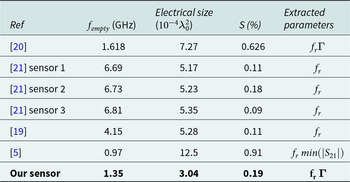
Table 3 presents a comparison of the proposed sensor with differential resonating sensors from the literature dedicated to small liquid volume analysis. For a better comparison, the electrical size of the sensing surface is expressed as a function of the squared wavelength $\lambda_0^2$ corresponding to the empty resonator resonance frequency $f_{empty}$. The sensitivity is calculated for all sensors from the measurement of water–ethanol mixtures by averaging the relative sensitivities of the resonance frequency obtained with all the measured samples (of ethanol concentration varying from $0\%$ to $100\%$). Air has been chosen as reference sample for this characterization. Our sensor exhibits an average relative sensitivity [Reference Liu, Zhang and Huang19] $S = 0.19\%$ that is close to that of other differential resonating sensors of similar sensitive area. This table also highlights the extracted parameters. A major contribution of this paper lies in the presented post-processing approach that permits to extract both resonance frequencies and widths in all loading conditions, even in the case of strong overlap.

Table 3.

Comparative table of differential resonating sensors for liquid measurement

Table 3 Long description

The table compares differential resonating liquid sensors by empty resonant frequency in gigahertz, electrical size, sensitivity in percent, and which measurement outputs were extracted. Our sensor is the most compact, with an electrical size of 3.04, an empty frequency of 1.35 gigahertz, and sensitivity of 0.19 percent, extracting both resonant frequency and a coupling related parameter. Reference 5 reports the highest sensitivity at 0.91 percent but also the largest electrical size at 12.5, with an empty frequency of 0.97 gigahertz and extraction based on resonant frequency and a transmission magnitude minimum. Reference 20 has an empty frequency of 1.618 gigahertz, electrical size 7.27, and sensitivity 0.626 percent, extracting resonant frequency and the coupling related parameter. The three sensors in reference 21 cluster near 6.7 to 6.81 gigahertz with electrical sizes about 5.17 to 5.35 and low sensitivities from 0.09 to 0.18 percent, extracting resonant frequency only. Reference 19 sits at 4.15 gigahertz, electrical size 5.28, and sensitivity 0.11 percent, also extracting resonant frequency only. Sensitivity does not increase consistently with frequency or size, so comparisons should be interpreted as reported values that may reflect different designs and extraction methods.

Due to the use of small liquid volumes, the impact of liquid evaporation as well as loading volume uncertainty on the extracted resonance frequencies has been evaluated through repeatability studies. Two loading conditions are considered with air as reference and water or ethanol as loading samples, and 25 successive measurements including the sample insertion step are carried out in each case. Whereas the highest resonance frequency (related to air) is very stable, with a normalized standard deviation of $2.3 \times 10^{-5}$ with water and $3.0 \times 10^{-4}$ with ethanol, higher variations are observed for the lowest resonance frequencies, with normalized standard deviations of $3.8 \times 10^{-3}$ with water and $4.6 \times 10^{-3}$ with ethanol.

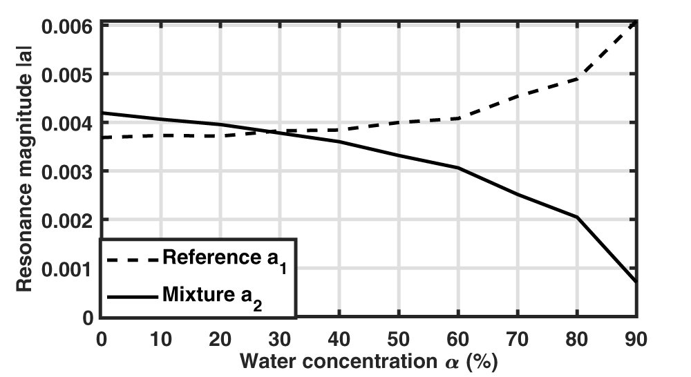
In addition to resonance frequencies and widths, the extraction method also leads to the values of $a_1$ and $a_2$ coefficients whose modulus are presented in Fig. 8. Whereas similar magnitudes are obtained up to 50 $\%$ of water, a discrepancy is then observed between both amplitudes, which complicates the extraction of the second resonance due to its lower amplitude. In particular, with 90 $\%$ of water, the magnitude ratio between $a_2$ and $a_1$ is 0.11. In order to understand this imbalance in excitation of both resonance modes, their associated field distributions have been studied.

Figure 8.

Magnitude of $a_1$ and $a_2$ coefficients as a function of the mixture water concentration.

Figure 8 Long description

The horizontal axis label is Water concentration alpha (percent). The horizontal axis range is 0 to 90. The vertical axis label is Resonance magnitude absolute value. The vertical axis range is 0 to 0.006. Legend: Reference a subscript 1; Mixture a subscript 2. Reference a subscript 1 coordinate pairs: (0, 0.0037), (10, 0.00375), (20, 0.00375), (30, 0.00385), (40, 0.00385), (50, 0.0040), (60, 0.0041), (70, 0.0046), (80, 0.0049), (90, 0.0060) Mixture a subscript 2 coordinate pairs: (0, 0.0042), (10, 0.0041), (20, 0.0040), (30, 0.0038), (40, 0.0036), (50, 0.0033), (60, 0.0031), (70, 0.0025), (80, 0.0020), (90, 0.0008).

Resonance mode properties

In order to study the resonance mode properties, both coupled SRRs have been simulated without the excitation microstrip line using the eigenmode solver of Ansys HFSS software (Fig. 9). Liquid dielectric properties have been modeled using the Debye model along with mixing laws for the mixtures (Eqs. 1–4). For each loading condition, two eigenvalues (complex eigenfrequencies) and eigenvectors (electric field distributions) are determined. It should be noted that eigenvectors are known up to a multiplicative constant; the field distributions are presented here for a stored energy of 1 joule within the simulated volume. Moreover, due to leakages in the materials (substrate and liquids), a global phase choice has been made to obtain a globally minimized nonuniform imaginary part of the $E_z$ component compared to its real part. The ensuing imaginary part being so small in all cases, we opted to present only the real parts in the following.

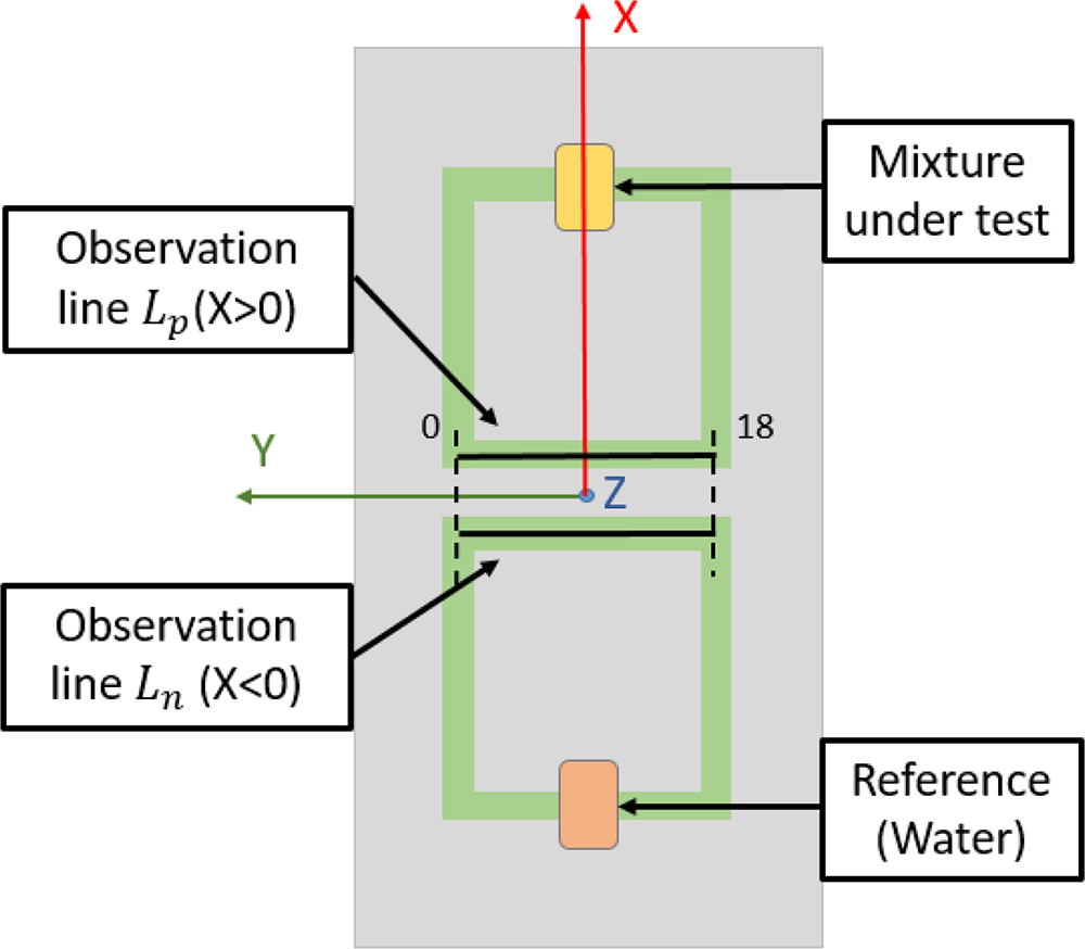
In order to highlight the field distribution differences between both resonators, two 18mm-long observation lines $L_n$ and $L_p$ parallel to the Y-axis are placed at the interface between the substrate and the resonators’ metallic strips (Fig. 9); the position of both observation lines has been chosen for their proximity with the microstrip excitation line (not simulated here) to establish a link with the excited mode amplitudes shown in the previous section (Fig. 8). Simulations are performed with deionized water as the reference sample (cavity at $X \lt 0$) and different water–ethanol mixtures (cavity at $X \gt 0$). Two different cases of water–ethanol mixtures are studied, one with water concentration 30 $\%$ and the other one with water concentration 90 $\%$. 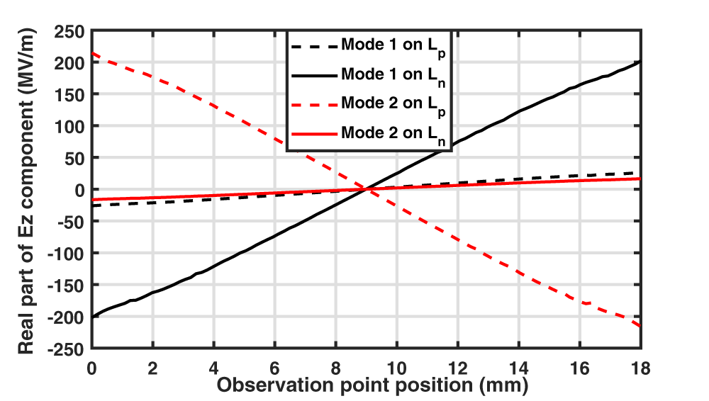The eigenmode electric field amplitudes are presented in Fig. 10, whereas the real part of $E_z$ component along both observation lines is presented in Fig. 11 with the 30W70E mixture and in Fig. 12 with the 90W10E mixture.

Figure 9.

Simulated structure using eigenmode solver and definition of both observation lines for electric field distribution.

Figure 9 Long description

This schematic diagram illustrates the setup for observing electric field distribution using two observation lines. The lines are labeled L subscript p left parenthesis X greater than 0 right parenthesis and L subscript n left parenthesis X less than 0 right parenthesis, positioned horizontally across the central region. The upper line, L subscript p and the lower line, L subscript n, serve as measurement paths for field distribution. Both lines connect via green conductors to blocks labeled 'Mixture under test' at the top and 'Reference left parenthesis Water right parenthesis' at the bottom, indicating a comparison between the mixture and water reference. The diagram features three axes: the X-axis is vertical and red, the Y-axis is horizontal and green and the Z-axis is marked on the horizontal line. Numeric markers '0' and '18' are visible along the observation lines, denoting specific positions or scales. The setup is enclosed within a rectangular boundary, with all components clearly labeled for reference.

Figure 10.

Electric field amplitude in the XOZ plane of both eigenmodes with an SRR (at $X \gt 0$) loaded with a water–ethanol mixture (30W70E or 90W10E) and the reference SRR (at $X \lt 0$) with deionized water.

Figure 10 Long description

The figure presents four electric field amplitude maps in the XOZ plane, arranged as two conditions each containing two eigenmodes. The color scale on the right is labeled E Field in V m superscript -1, ranging from 0.00E plus 00 at the lower end to 1.39E plus 08 at the upper end, with intermediate labeled values of 1.20E plus 07, 2.39E plus 07, 3.59E plus 07, 4.79E plus 07, 5.98E plus 07, 7.18E plus 07, 8.38E plus 07, 9.57E plus 07, 1.08E plus 08, 1.20E plus 08 and 1.32E plus 08. The horizontal axis represents the X direction and the vertical axis represents the Z direction within the XOZ plane. No dimensional units are labeled on the spatial axes. Mode 1 under Water 30W70E has a resonant frequency of 1.21 GHz. The field amplitude is concentrated in a localized region near the inner edge of the split-ring resonator gap. Mode 1 under Water 90W10E also has a resonant frequency of 1.21 GHz. The spatial distribution of the field hotspot is similar in location to the Water 30W70E Mode 1 case, appearing near the resonator gap region. Mode 2 under Water 30W70E has a resonant frequency of 1.28 GHz. The field hotspot is more intense and more spatially concentrated near the resonator gap compared to Mode 1. Mode 2 under Water 90W10E has a resonant frequency of 1.23 GHz, which is lower than the 1.28 GHz observed for Mode 2 under Water 30W70E, indicating a frequency shift between the two mixture conditions. Water 30W70E denotes 30 percent water and 70 percent ethanol. Water 90W10E denotes 90 percent water and 10 percent ethanol. A diagonal red line visible in each map represents an observation path along which the field is sampled parallel to the Y-axis, placed at the interface between the substrate and the resonator metallic strip. A red X mark in each map indicates the reference point or start location along that observation line.

Figure 11.

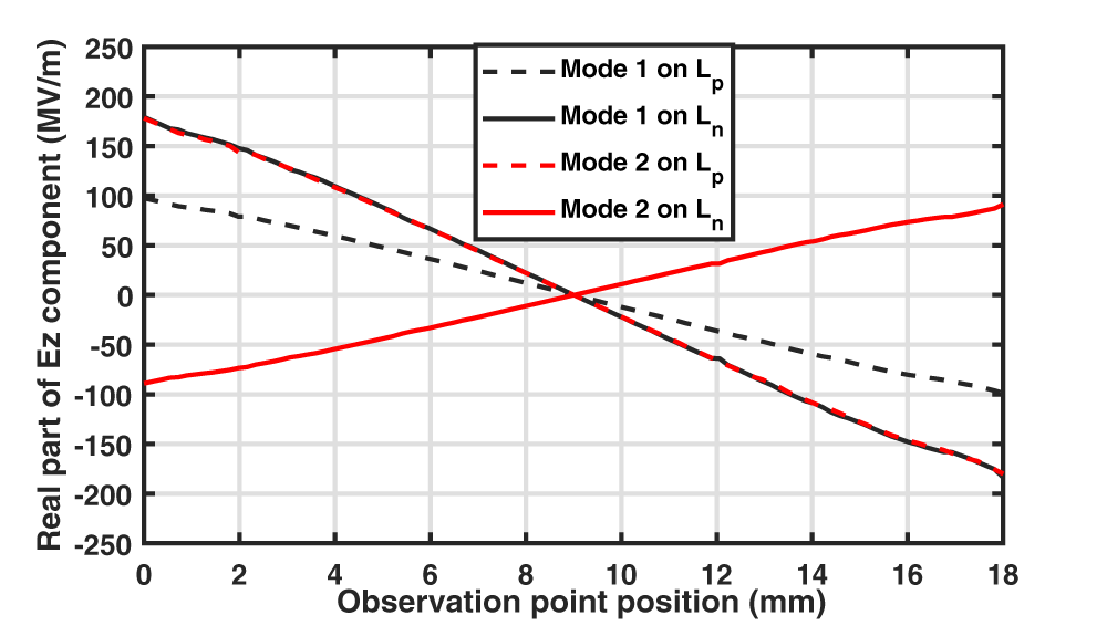
Real part of the $E_z$ electric field component for both eigenmodes when an SRR (at $X \gt 0$) is loaded with the 30W70E mixture and the reference SRR (at $X \lt 0$) with deionized water. For each eigenmode, the electric field variation is observed on $L_n$ and on $L_p$ lines, respectively, on the resonator at X $ \lt 0$ and at X $ \gt 0$.

Figure 11 Long description

Real part of Ez component (MV/m) Observation point position (mm) Legend: Mode 1 on Lp; Mode 1 on Ln; Mode 2 on Lp; Mode 2 on Ln. Horizontal axis label: Observation point position (mm). Range: 0 to 18. Vertical axis label: Real part of Ez component (MV/m). Range: negative 250 to 250. Mode 1 on Ln: (0, negative 200), (18, 200) Mode 2 on Lp: (0, 220), (18, negative 220) Mode 1 on Lp: (0, negative 25), (18, 30) Mode 2 on Ln: (0, negative 15), (18, 20).

Figure 12.

Real part of the $E_z$ electric field component for both eigenmodes when an SRR (at $X \gt 0$) is loaded with the 90W10E mixture and the reference SRR (at $X \lt 0$) with deionized water. For each eigenmode, the electric field variation is observed on $L_n$ and on $L_p$ lines, respectively, on the resonator at X $ \lt 0$ and at X $ \gt 0$.

Figure 12 Long description

Real part of Ez component (MV/m) A line graph with a legend listing four series: “Mode 1 on Lp” (dashed), “Mode 1 on Ln” (solid), “Mode 2 on Lp” (dashed) and “Mode 2 on Ln” (solid). The x-axis is labeled “Observation point position (mm)”, ranging from 0 to 18 with tick marks at 0, 2, 4, 6, 8, 10, 12, 14, 16 and 18. The y-axis is labeled “Real part of Ez component (MV/m)”, ranging from minus 250 to 250 with tick marks every 50. Mode 1 on Lp (dashed): about 100 at 0 mm, about 80 at 2 mm, about 60 at 4 mm, about 40 at 6 mm, about 20 at 8 mm, about 0 at 10 mm, about minus 30 at 12 mm, about minus 55 at 14 mm, about minus 80 at 16 mm and about minus 100 at 18 mm. Mode 1 on Ln (solid): about 180 at 0 mm, about 150 at 2 mm, about 110 at 4 mm, about 65 at 6 mm, about 20 at 8 mm, about minus 20 at 10 mm, about minus 65 at 12 mm, about minus 110 at 14 mm, about minus 150 at 16 mm and about minus 180 at 18 mm. Mode 2 on Lp (dashed): the curve closely overlaps the “Mode 1 on Ln” solid curve across the full range, starting near 180 at 0 mm and ending near minus 180 at 18 mm, with a crossing near 9 mm at about 0. Mode 2 on Ln (solid): about minus 90 at 0 mm, about minus 75 at 2 mm, about minus 55 at 4 mm, about minus 30 at 6 mm, about minus 10 at 8 mm, about 10 at 10 mm, about 35 at 12 mm, about 55 at 14 mm, about 75 at 16 mm and about 95 at 18 mm.

In each loading case, the resonance frequencies of both eigenmodes are indicated. A difference is observed with the values obtained when both resonators are excited by a microstrip line. For instance, the resonance frequency of the first mode is 1.21 GHz instead of 1.18 GHz obtained from the transmission coefficient (Table 2). This discrepancy is explained by the modification of the resonators’ behavior and their mutual coupling due to the presence or absence of the microstrip line between them.

In all cases, the eigenmode of lower resonance frequency (mode 1) is associated with a higher electric field energy around the cavity loaded by the liquid having the highest permittivity real part which is water in this case (cavity at $X \lt 0$), whereas for mode 2 the electric field energy is higher around the cavity loaded by the mixture (cavity at $X \gt 0$). This is more marked when the dielectric properties of both samples are very different; for a mixture containing 30 $\%$ of water, the energy is principally localized around one cavity (at $X \lt 0$ for mode 1 and at $X \gt 0$ for mode 2) (Fig. 10). The real part of $E_z$ component is much higher along the observation line of the same resonator (that is $L_n$ for mode 1 and $L_p$ for mode 2) (Fig. 11). When the dielectric properties of both samples are closer (with a mixture containing 90 $\%$ of water), the field amplitudes around both cavities (Fig. 10) as well as along both observation lines (Fig. 12) are more similar.

Additionally, it is of interest to observe the sign of $E_z$ real part along $L_n$ and $L_p$ lines. For all loading conditions, the sign is the same on both observation lines for mode 1, whereas it is opposite for mode 2. As the $E_z$ field component generated by a microstrip line is symmetric with respect to the YOZ plane, the excitation field better couples to mode 1 following the same symmetry. The impact of these mode symmetry properties remains weak when the field principally concentrates in one single resonator (as with 30W70E mixture), but the excitation of mode 2 becomes more difficult when the $E_z$ real part on $L_n$ is no longer negligible (as with 90W10E mixture). 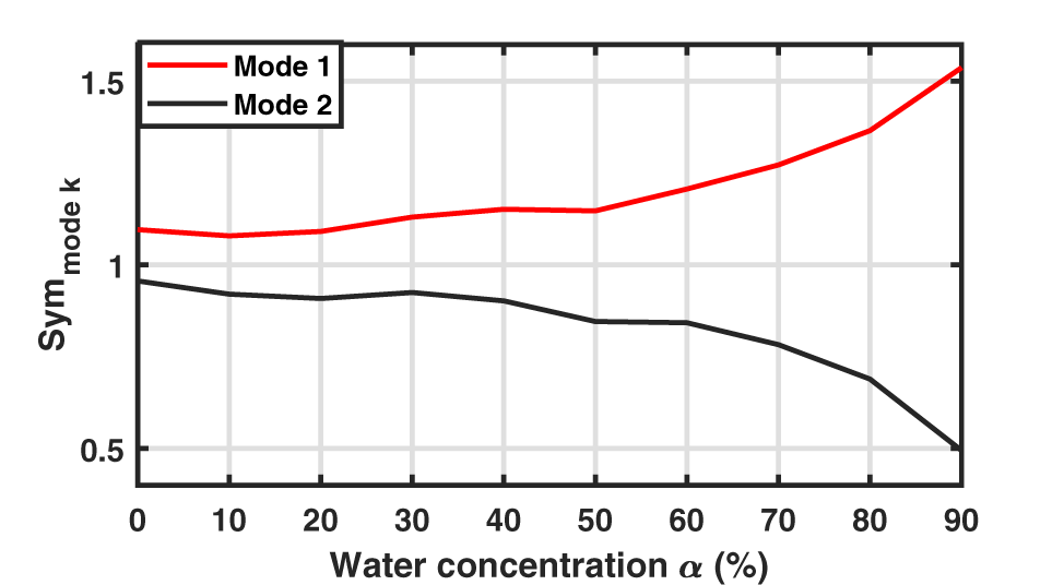It explains why the amplitude of $a_2$ is 8 times smaller than $a_1$ with the 90W10E sample, whereas very close amplitudes are obtained with the 30W70E one (Fig. 8). The symmetry properties of both modes for every tested mixture are presented in Fig. 13 using the following symmetry indicator:

(9)\begin{equation} Sym_{mode~k} = \frac{|E_{z,L_p,k,18mm}+E_{z,L_n,k,18mm}|}{max(|E_{z,L_p,k,18mm}|,|E_{z,L_n,k,18mm}|)}\,. \end{equation}

calculated using the complex $E_z$ field component at $L_n$ and $L_p$ right extremities (position 18mm) for each eigenmode k. The similar variation shape of this symmetry indicator with $a_1$ and $a_2$ amplitudes (Fig. 8) highlights the link between these symmetry properties and the excited mode amplitudes.

Figure 13.

Symmetry indicator of both eigenmodes calculated according to Eq. 9 when deionized water is used as reference sample and mixtures of different water concentrations are inserted in the other resonator.

Figure 13 Long description

A line graph with a legend listing Mode 1 and Mode 2. Horizontal axis label: Water concentration alpha (percent). Range: 0 to 90. Vertical axis label: Sym mode k. Range: 0.5 to 1.5. Mode 1: (0, 1.1), (10, 1.08), (20, 1.09), (30, 1.12), (40, 1.14), (50, 1.14), (60, 1.2), (70, 1.27), (80, 1.37), (90, 1.55) Mode 2: (0, 0.95), (10, 0.92), (20, 0.91), (30, 0.93), (40, 0.9), (50, 0.85), (60, 0.84), (70, 0.78), (80, 0.68), (90, 0.5).