1. Introduction
Understanding, predicting and controlling coherent instability structures in wall-bounded shear flows remain central challenges in fluid mechanics, especially for high-speed boundary layer transition. Resolvent analysis, which treats the linearised Navier–Stokes equations as an input–output system, has become an effective framework for identifying amplified flow responses and their associated forcing mechanisms (Trefethen et al. Reference Trefethen, Trefethen, Reddy and Driscoll1993; McKeon & Sharma Reference McKeon and Sharma2010; Towne et al. Reference Towne, Schmidt and Colonius2018). In compressible boundary layers, resolvent-based approaches have been used to clarify instability mechanisms such as the interaction between second-mode waves, non-modal streaks and other coherent structures in hypersonic flows (Jahanbakhshi & Zaki Reference Jahanbakhshi and Zaki2019; Bugeat et al. Reference Bugeat, Robinet, Chassaing and Sagaut2022; Madhusudanan et al. Reference Madhusudanan, Stroot and McKeon2025). In addition, resolvent gain sensitivity has provided useful guidance for passive surface deformation and active actuation design (Poulain et al. Reference Poulain, Content, Rigas, Garnier and Sipp2024; Gao et al. Reference Gao, Ma, Ren, Yuan and Zhang2025; Yuan et al. Reference Yuan, Kou, Zheng and Zhang2025).
Despite its physical interpretability, conventional resolvent analysis remains computationally demanding for high-dimensional parameter studies and control-oriented optimisation. Standard singular-value-decomposition-based resolvent computations require the construction and decomposition of large linear operators, and the cost becomes substantial for spatially resolved compressible flows (Gupta et al. Reference Gupta, Madhusudanan, Wan, Illingworth and Juniper2021). This bottleneck is especially severe when the base flow varies with Mach number, Reynolds number or control actuation, because the corresponding linearised operator must be repeatedly reconstructed and decomposed (Chen et al. Reference Chen, Cheng, Fu and Gan2023). Most conventional resolvent analyses proceed from a prescribed forcing to the corresponding response, whereas control-oriented design often starts from a desired response and seeks a compatible forcing. In the full field setting considered in the present study, however, both the target response and the discrete operator are known, so the compatible forcing is obtained directly by applying the operator. We therefore use the term ‘inverse problem’ only to describe the operational response to the forcing direction. Reconstruction from partial or noisy observations, with an unknown operator, or under actuator constraints, would define different problems that may become underdetermined or ill-conditioned; such settings are outside the scope of the present work.
Scientific machine learning offers a promising route for reducing this computational burden. Instead of learning finite-dimensional vectors only, neural operators aim to approximate mappings between function spaces and have shown strong potential for surrogate modelling of partial differential equations (Brunton et al. Reference Brunton, Noack and Koumoutsakos2020; Li et al. Reference Li, Kovachki, Azizzadenesheli, Liu, Bhattacharya, Stuart and Anandkumar2021; Lu et al. Reference Lu, Jin, Pang, Zhang and Karniadakis2021; Kovachki et al. Reference Kovachki, Li, Liu, Azizzadenesheli, Bhattacharya, Stuart and Anandkumar2023; Wang et al. Reference Wang2024). DeepONet-based models and related variants have been applied to complex fluid mechanics problems, including instability wave prediction and data assimilation in hypersonic boundary layers (Clark Di Leoni et al. Reference Clark Di Leoni, Lu, Meneveau, Karniadakis and Zaki2023). Transformer architectures (Vaswani et al. Reference Vaswani, Shazeer, Parmar, Uszkoreit, Jones, Gomez, Kaiser and Polosukhin2017), with their capability to capture long-range dependencies, have also been adapted to physical field prediction. Representative Transformer-based neural operators include the Galerkin Transformer and OFormer, alongside GNOT for multiple inputs and irregular meshes, GINOT for arbitrary geometries represented by boundary point clouds, and S-NOT for sequential inputs in time-dependent nonlinear problems (Cao Reference Cao2021; Li et al. Reference Li, Meidani and Farimani2023; Hao et al. Reference Hao, Wang, Su, Ying, Dong, Liu, Cheng, Song and Zhu2023; Liu et al. Reference Liu, Zhong, Koric and Meidani2026a , Reference Liu, Zhong, Meidani, Abueidda, Koric and Geubelle2026b ). Of particular relevance to the present work, the physics attention mechanism in Transolver (Wu et al. Reference Wu, Luo, Wang, Wang and Long2024) provides an efficient way to aggregate grid point information into physics-aware tokens and is therefore well suited for parameter-conditioned flow field mappings. Physics-informed learning further enables data-driven models to incorporate governing equation residuals into the training objective (Raissi, Perdikaris & Karniadakis Reference Raissi, Perdikaris and Karniadakis2019). However, the joint optimisation of data fitting and physics-based objectives may suffer from imbalance and competing training requirements, motivating stabilised formulations based on improved residual construction and multi-objective optimisation strategies (Yang et al. Reference Yang, Qian, Hang and Liu2025). Although neural operators have recently been explored in resolvent-related modelling (Wu et al. Reference Wu, Zhang and He2025), a unified framework that combines forward resolvent response prediction, inverse forcing reconstruction, physics-informed matrix consistency and realisable flow control guidance remains limited.
In this study, we propose a Transformer-based neural resolvent operator framework, termed ResFormer, for forward and inverse modelling of compressible boundary layer instability waves. The framework is designed to learn parameter-conditioned mappings among base-flow states, harmonic forcing fields and resolvent responses. The remainder of this paper is organised as follows. Section 2 introduces the physical model, the harmonic resolvent formulation, the numerical case summary and the ResFormer neural operator framework. Section 3 evaluates the forward approximation and parameter interpolation performance of ResFormer. Section 4 extends the framework from forward prediction to data-driven inverse forcing reconstruction. To further improve the physical consistency of inverse prediction, § 5 introduces a physics-informed inversion strategy for spatially attenuated instability waves. Building on these forward and inverse capabilities, § 6 presents a numerical validation of realisable flow control guidance, where the ideal inverse forcing is reduced to a compact wall-normal blowing/suction actuator and evaluated using high-fidelity computational fluid dynamics (CFD) simulations through lock-in processing and modal projection. Finally, § 7 summarises the main findings and discusses future extensions towards efficient stability databases and surrogate-assisted active flow control design.
2. Problem formulation and ResFormer methodology
2.1. Physical model and resolvent formulation
We consider the compressible flow over a flat plate governed by the linearised Navier–Stokes (LNS) equations in conservative form. The governing system is derived by linearising the full compressible equations about a two-dimensional steady base flow
 $\overline {\boldsymbol{q}}$
. The resulting conservative perturbation state vector,
 $\boldsymbol{q}'$
, comprises fluctuations of density, streamwise, wall-normal and spanwise momentum, and total energy. The LNS system can be expressed in compact form as
 \begin{align} \frac {\partial \boldsymbol{q}'}{\partial t}= \mathcal{L}(\overline {\boldsymbol{q}}) \boldsymbol{q}'+ \boldsymbol{f}', \end{align}
where
 $\mathcal{L}$
denotes the linearised Navier–Stokes operator, including both inviscid and viscous contributions evaluated about the base flow, and
 $\boldsymbol{f}'$
represents an external forcing term.
Assuming harmonic disturbances of the form
 $ (\boldsymbol{q}',\boldsymbol{f}')=(\hat {\boldsymbol{q}},\kern2.5pt \hat {\boldsymbol{\kern-2.5pt f}}) \,\text{e}^{{i}(\beta z+\omega t)},$
where
 $\omega$
and
 $\beta$
denote the angular frequency and spanwise wavenumber, respectively, substitution into (2.1) yields the harmonic LNS system
 \begin{align} \left ( \mathrm{i}\omega \boldsymbol{I}-\mathcal{L}_{\beta } \right ) \hat {\boldsymbol{q}}=\kern2.5pt \hat {\boldsymbol{\kern-2.5pt f}}, \end{align}
where
 $\mathcal{L}_{\beta }$
denotes the spanwise wavenumber-dependent harmonic LNS operator.
After spatial discretisation, equation (2.2) can be written as
 $\boldsymbol{A}_{\omega ,\beta }\hat {\boldsymbol{q}}=\kern2.5pt \hat {\boldsymbol{\kern-2.5pt f}}$
, where
 $\boldsymbol{A}_{\omega ,\beta }$
denotes the complete discrete harmonic LNS operator. The corresponding resolvent operator is defined as
 \begin{align} \hat {\boldsymbol{q}}=\mathcal{H}(\omega ,\beta ,\overline {\boldsymbol{q}}) \kern2.5pt \hat {\boldsymbol{\kern-2.5pt f}}=\boldsymbol{A}_{\omega ,\beta }^{-1} \kern2.5pt \hat {\boldsymbol{\kern-2.5pt f}}, \end{align}
where
 $\mathcal{H}$
represents the forcing-to-response mapping associated with the base flow
 $\overline {\boldsymbol{q}}$
.
In the classical resolvent framework, the optimal forcing and response are obtained from the leading singular vectors of the resolvent operator
 $\mathcal{H}$
through singular-value decomposition (SVD), while the corresponding singular value represents the maximum amplification gain. The resulting optimal forcing response pairs constitute the reference datasets used throughout this work. Throughout the paper,
 $\boldsymbol{A}_{\omega ,\beta }$
denotes the discrete harmonic LNS operator, whereas
 $\mathcal{H}=\boldsymbol{A}_{\omega ,\beta }^{-1}$
denotes the corresponding resolvent operator. The discretised harmonic LNS operator and the reference resolvent datasets are constructed using the BROADCAST-based resolvent analysis framework developed by Poulain et al. (Reference Poulain, Content, Sipp, Rigas and Garnier2023).
The numerical cases investigated in this study cover supersonic and hypersonic boundary layers, including laminar, turbulent and actively controlled configurations. Table 1 summarises the cases in the present study. The first six rows correspond to neural operator training or evaluation tasks, while the CFD simulations case is used as a realisable control validation to connect the inverse forcing prediction with boundary actuation.
Summary of numerical cases and their roles in this study.

Table 1. Long description
The table has seven rows and four columns. The columns are labeled Case, Flow condition, Main variation, and Task. The rows are labeled with different cases: F, S, M, T, BS, PI, and CFD simulations. Each row provides details about the flow condition, main variation, and task for each case. For example, Case F involves a laminar boundary layer with a Mach number of 4.5 and focuses on forward TS-wave prediction. Case S also involves a laminar boundary layer with a Mach number of 4.5 but focuses on second-mode prediction. Case M involves a laminar boundary layer with Mach numbers ranging from 3.0 to 4.5 and focuses on Mach-number interpolation. Case T involves a turbulent boundary layer with a Mach number of 2.25 and focuses on data-driven inverse forcing reconstruction. Case BS involves a blowing/suction boundary layer with a Mach number of 5.86 and focuses on data-driven inverse forcing reconstruction. Case PI involves spatially attenuated instability waves with a Mach number of 4.5 and focuses on physics-informed inverse forcing. The CFD simulations case involves upstream forced TS response and focuses on realisable wall control validation.
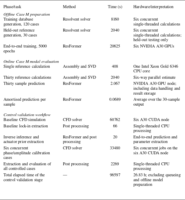
Detailed numerical parameters, data partitions, attenuation target sampling settings and implementation details are provided in Appendix A. A supplementary wall-clock efficiency comparison is given in Appendix B.
2.2. The ResFormer architecture
The overall ResFormer framework is illustrated in figure 1. Starting from a prescribed compressible boundary layer configuration, the base flow
 $\overline {\boldsymbol{q}}$
and modal parameters
 $(\omega ,\beta )$
are used to construct harmonic resolvent data. In this study, the reference resolvent fields are generated following the BROADCAST-based resolvent analysis framework (Poulain et al. Reference Poulain, Content, Sipp, Rigas and Garnier2023). The resulting data include forcing response pairs
 $(\kern2.5pt \hat {\boldsymbol{\kern-2.5pt f}},\hat {\boldsymbol{q}})$
and optimal mode targets
 $(\hat {\boldsymbol{q}}_{\textit{opt}},\kern2.5pt \hat {\boldsymbol{\kern-2.5pt f}}_{\textit{opt}})$
. For inverse control-oriented studies, prescribed attenuation targets
 $\hat {\boldsymbol{q}}_{\textit{target}}$
are subsequently constructed from these reference responses using spatial masks. The neural operator backbone is adapted from the physics attention Transformer architecture of Transolver (Wu et al. Reference Wu, Luo, Wang, Wang and Long2024).
Overall ResFormer framework for forward and inverse resolvent modelling. The physical set-up and base flow are first used to generate harmonic resolvent datasets. ResFormer then learns three parameter-conditioned operator mappings: forcing-to-response approximation, rapid optimal mode prediction and response-to-forcing reconstruction for prescribed target responses.

ResFormer is designed to learn parameter-conditioned field-to-field mappings. Compared with conventional convolution-based networks, the physics attention mechanism first aggregates grid point features into physics-aware tokens, applies attention in a latent physical space and then projects the learned information back to the physical domain. This structure is suitable for resolvent mode prediction because instability waves involve long-range streamwise correlations, multi-scale spatial structures and strong dependence on modal parameters.
As shown in figure 1, the framework contains three operator learning pathways. The first pathway approximates the forward resolvent mapping from forcing to response,
 \begin{align} \mathcal{G}_{\textit{op}}: ( \kern2.5pt \hat {\boldsymbol{\kern-2.5pt f}}, \omega , \beta ) \rightarrow \hat {\boldsymbol{q}} . \end{align}
This pathway directly learns the forcing-to-response relation associated with the resolvent operator. It is used to evaluate whether the neural operator can reproduce the linear response of the flow to prescribed harmonic forcing.
The second pathway performs rapid optimal mode prediction,
 \begin{align} \mathcal{G}_{\textit{pred}}: ( \overline {\boldsymbol{q}}, \omega , \beta ) \rightarrow \big( \hat {\boldsymbol{q}}_{\textit{opt}}, \kern2.5pt \hat {\boldsymbol{\kern-2.5pt f}}_{\textit{opt}} \big). \end{align}
Instead of performing a new SVD-based resolvent computation for each parameter combination, this pathway maps the base-flow state and modal parameters directly to the corresponding optimal response and forcing. It therefore provides a fast surrogate for constructing high-resolution modal databases.
The third pathway is a response-to-forcing reconstruction model, denoted by
 \begin{align} \mathcal{G}_{\textit{in}v}: \big( \hat {\boldsymbol{q}}_{\textit{target}}, \omega , \beta \big) \rightarrow \kern2.5pt \hat {\boldsymbol{\kern-2.5pt f}}_{\textit{in}v} . \end{align}
This pathway learns a surrogate response-to-forcing mapping for control-oriented guidance. When the prescribed target response is the optimal resolvent response,
 $\kern2.5pt \hat {\boldsymbol{\kern-2.5pt f}}_{\textit{in}v}$
corresponds to the associated optimal forcing
 $\kern2.5pt \hat {\boldsymbol{\kern-2.5pt f}}_{\textit{opt}}$
. When the target is a spatially attenuated response,
 $\kern2.5pt \hat {\boldsymbol{\kern-2.5pt f}}_{\textit{in}v}$
represents the compatible volumetric forcing under the discrete harmonic LNS formulation.
All supervised models employ a relative
 $L_2$
objective. The detailed architecture and optimisation settings, the precise samplewise averaging convention and the random seed sensitivity analysis are provided in Appendix A.2.
3. Forward resolvent operator approximation and parameter interpolation
3.1. Capturing instability modes
This section validates the capability of ResFormer to capture instability mechanisms across distinct spectral regimes, ranging from low-frequency Tollmien–Schlichting (TS) waves to high-frequency second-mode (Mack mode) instabilities. Case F evaluates low-frequency TS-wave responses by varying
 $\beta$
at fixed
 $\omega$
, whereas Case S evaluates high-frequency second-mode responses by varying
 $\omega$
at
 $\beta =0$
. The optimal forcing at
 $ \textit{Ma}=4.5$
and
 $ \textit{Re}_u=3.4\times 10^6$
serves as the model input, with the corresponding optimal response designated as the prediction target.
To quantify the prediction accuracy, we use a consistent global
 $L_2$
response norm for both the ground truth (GT) and the prediction:
 \begin{align} \mu _{L_2}= \left \| \hat {\boldsymbol{q}} \right \|_{\varOmega }= \left ( \int _{\varOmega } \sum _{i=1}^{5} | \hat {q}_i |^2 \,\mathrm{d}\varOmega \right )^{\!1/2} \!, \end{align}
where
 $\hat {q}_i$
denotes the conservative variable components of
 $\hat {\boldsymbol{q}}$
. This metric is used because the neural network predicts conservative variables directly. It provides a consistent amplitude measure for comparing predicted and reference response fields in the same variable representation.
Unless otherwise stated, the reported prediction error is the mean samplewise relative
 $L_2$
error defined in (A2). The modal field errors reported in figures 2(c) and 3(c) are evaluated using spatial quadrature, with the arbitrary global modal sign aligned where applicable. Random seed variability for representative forward and inverse tasks is reported in table 8.
As shown in figures 2 and 3, ResFormer accurately reconstructs the global response amplitude, mode profile, peak location and spatial structure. Figures 2(a) and 3(a) compare the reference and predicted global response norms, whereas figures 2(c) and 3(c) report the spatially weighted relative
 $L_2$
error of the complete five-component response field at the test points distributed throughout the training parameter range. For Case F, the mean relative error of the predicted response norm
 $\mu _{L_2}$
is
 $0.16\,\%$
, and the mean relative
 $L_2$
field error is
 $0.0096$
. The near-wall TS wavepacket and its streamwise evolution are accurately reproduced. For Case S, the corresponding mean errors are
 $0.034\,\%$
for
 $\mu _{L_2}$
and
 $0.0026$
for the complete response field. The predicted field also reproduces the acoustic mode structures trapped inside the boundary layer. The agreement at the distributed test points demonstrates that ResFormer maintains good interpolation accuracy throughout the considered training parameter ranges.
Forward prediction for Case F (TS instability). (a) Global response norm
 $\mu _{L_2}$
as a function of spanwise wavenumber
 $\beta$
at
 $\omega =1.0\times 10^{-5}$
. The black dashed line denotes the reference result, and the red hollow circles denote the ResFormer predictions at the test points distributed throughout the training parameter range. (b) Reference and predicted density mode profiles at
 $ \textit{Re}_y=1.12\times 10^4$
for the representative interpolation sample
 $(\omega =1.0\times 10^{-5},\ \beta =2.2\times 10^{-4})$
. (c) Spatially weighted relative
 $L_2$
error of the complete five-component response field at the distributed test points; the black dashed line denotes the mean value. (d–f) Reference density fluctuation field, prediction and pointwise absolute error field for the same representative sample.

Forward prediction for Case S (second-mode instability) at
 $ \textit{Ma}=4.5$
and
 $\beta =0$
. (a) Global response norm
 $\mu _{L_2}$
as a function of frequency
 $\omega$
. The black dashed line denotes the reference result, and the red hollow circles denote the ResFormer predictions at the test points distributed throughout the training parameter range. (b) Reference and predicted density mode profiles at
 $ \textit{Re}_y=8.78\times 10^3$
for the representative interpolation sample
 $\omega =3.1\times 10^{-4}$
. (c) Spatially weighted relative
 $L_2$
error of the complete five-component response field at the distributed test points; the black dashed line denotes the mean value. (d–f) Reference density fluctuation field, prediction and pointwise absolute error field for the same representative sample.

Figure 3. Long description
Panel A: A line graph shows the global response norm as a function of frequency. The x-axis is labeled with frequency (fω) in units of 10^-4, and the y-axis is labeled with the global response norm (μL2) in units of 10^6. The black dashed line represents the ground truth, and the red hollow circles denote the ResFormer predictions at test points. Panel B: A line graph displays the reference and predicted density mode profiles. The x-axis is labeled with Re_x in units of 10^5, and the y-axis is labeled with density (ρ). The blue line represents the reference, and the red line represents the prediction. Panel C: A scatter plot shows the spatially weighted relative error of the complete five-component response field at distributed test points. The x-axis is labeled with frequency (fω) in units of 10^-4, and the y-axis is labeled with the relative error (εrelL2). The red circles denote test samples, and the black dashed line denotes the mean value. Panel D: A heatmap shows the reference density fluctuation field. The x-axis is labeled with Re_x in units of 10^5, and the y-axis is labeled with Re_y. The color scale ranges from -600 to 600. Panel E: A heatmap shows the predicted density fluctuation field. The x-axis is labeled with Re_x in units of 10^5, and the y-axis is labeled with Re_y. The color scale ranges from -600 to 600. Panel F: A heatmap shows the pointwise absolute error field. The x-axis is labeled with Re_x in units of 10^5, and the y-axis is labeled with Re_y. The color scale ranges from 0 to 2.
As an additional architecture baseline, Case S was evaluated using the Fourier neural operator (FNO) of Li et al. (Reference Li, Kovachki, Azizzadenesheli, Liu, Bhattacharya, Stuart and Anandkumar2021), implemented with the official Neural Operator package (Kossaifi et al. Reference Kossaifi2025). In a separate fixed budget comparison, both FNO and ResFormer were trained for 5000 epochs using the same dataset, train test split, preprocessing, optimiser settings and unweighted samplewise relative
 $L_2$
loss. Under this common budget, ResFormer (
 $0.274$
M parameters) achieved a relative
 $L_2$
error of
 $1.443\,\%\pm 0.069\,\%$
, whereas FNO (
 $0.505$
M parameters) achieved
 $2.713\,\%\pm 0.128\,\%$
. Thus, ResFormer attained a lower fixed budget error despite using fewer trainable parameters. Further details are provided in table 9.
3.2. Mach-number interpolation
Following the validation of frequency-regime instabilities, we assess the model’s interpolation capability under Mach-number-induced base-flow variations. For Case M, the Mach number varies within
 $ \textit{Ma} \in [3.0, 4.5]$
while keeping
 $ \textit{Re}_u = 3.4 \times 10^6$
,
 $\omega = 1.0 \times 10^{-5}$
and
 $\beta = 1.0 \times 10^{-5}$
fixed.
As shown in figure 4, ResFormer smoothly interpolates the variation of the instability response with Mach number. For the displayed interpolation test points, the mean relative error of the global response norm
 $\mu _{L_2}$
is
 $0.50\,\%$
, while the mean spatially weighted relative
 $L_2$
error of the complete five-component response field is
 $0.0231$
. The predicted response amplitude curve agrees closely with the reference data. Despite the variations in boundary layer thickness and mode structure induced by compressibility effects, the model accurately preserves the spatial distribution and streamwise evolution of the momentum fluctuation
 $\widehat {\rho u}$
. These results demonstrate good interpolation accuracy within the considered Mach-number range and suggest that a relatively sparse sampling of the flow parameter space may be used to construct high-resolution stability databases at reduced computational cost.
Additional norm-sensitive effective gain and response alignment diagnostics for Case M are reported in Appendix C.2.
Mach-number interpolation for Case M. (a) Global response norm
 $\mu _{L_2}$
as a function of Mach number over
 $ \textit{Ma}\in [3.0,4.5]$
. The black dashed line denotes the reference result, and the red hollow circles denote ResFormer predictions at the displayed interpolation test points. (b) Reference and predicted streamwise momentum fluctuation profiles
 $\widehat {\rho u}$
at
 $ \textit{Re}_y=7.52\times 10^3$
for the representative test sample
 $ \textit{Ma}=3.50$
. (c) Spatially weighted relative
 $L_2$
error of the complete five-component response field at the displayed test points; the black dashed line denotes the mean value. (d–f) Reference streamwise momentum fluctuation field, prediction and pointwise absolute error field for the same representative sample.

The present evaluation focuses on Mach-number interpolation over
 $ \textit{Ma}\in [3.0,4.5]$
at a fixed Reynolds number. Because these cases retain a consistent family of boundary layer states and instability structures, the results demonstrate the predictive capability of ResFormer for unseen Mach-number conditions within the represented flow family. A substantial Reynolds-number variation may additionally modify the viscous scaling and instability spectrum or activate a different instability branch. Extension to such topology-changing regimes can be achieved through targeted database enrichment, adaptive sampling or transfer learning using representative samples from the newly encountered regime.
Inverse forcing reconstruction for the supersonic turbulent boundary layer at
 $ \textit{Ma}=2.25$
(Case T). (a) Global forcing norm
 $\|\kern2.5pt \hat {\boldsymbol{\kern-2.5pt f}}\|_{\varOmega }$
as a function of spanwise wavenumber
 $\beta$
at
 $\omega =1.0\times 10^{-5}$
. The black dashed line denotes the reference result, and the red hollow circles denote ResFormer predictions on the test set. (b) Reference and predicted profiles of the streamwise momentum forcing component
 $f_{\rho u}$
at
 $ \textit{Re}_y=5.29\times 10^3$
for the representative test sample
 $(\omega =1.0\times 10^{-5},\ \beta =1.92\times 10^{-4})$
. (c) Spatially weighted relative
 $L_2$
error of the complete five-component forcing field at the test points; the black dashed line denotes the mean value. (d–f) Reference
 $f_{\rho u}$
forcing field, prediction and pointwise absolute error field for the same representative sample.

Figure 5. Long description
Panel A: A line graph shows the global forcing norm as a function of spanwise wavenumber. The x-axis is labeled ‘Wavenumber β’ with units in 10^-4, and the y-axis is labeled ‘Forcing norm ||f||2’ with units in 10^-1. The black dashed line represents the reference result, and the red hollow circles denote ResFormer predictions on the test set. Panel B: A line graph displays the reference and predicted profiles of the streamwise momentum forcing component. The x-axis is labeled ‘Re_x’ with units in 10^6, and the y-axis is labeled ‘f_rho u’. The blue line represents the reference, and the red line represents the prediction. Panel C: A scatter plot shows the spatially weighted relative error of the complete five-component forcing field at the test points. The x-axis is labeled ‘Wavenumber β’ with units in 10^-4, and the y-axis is labeled ‘ε_rel L2’. The red circles denote test samples, and the black dashed line denotes the mean value. Panels D, E, and F: Heatmaps illustrate the reference forcing field, prediction, and pointwise absolute error field. The x-axis is labeled ‘Re_x’ with units in 10^6, and the y-axis is labeled ‘Re_y’ with units in 10^4. The color scale indicates the magnitude of the forcing field or error.
4. Data-driven inverse forcing reconstruction
4.1. Inverse forcing reconstruction over a turbulent mean flow
Beyond forward prediction, ResFormer is used for data-driven response-to-forcing reconstruction. It learns the mapping from prescribed response fields to their associated forcing fields, and identifies the dominant forcing structures in the investigated configurations. Here, we apply ResFormer to a supersonic turbulent boundary layer at
 $ \textit{Ma}=2.25$
to reconstruct the forcing fields corresponding to resolvent response modes across a range of spanwise wavenumbers. Unlike Case M, the mean flow profile remains fixed; consequently, the network must uniquely distinguish variations in the forcing field from changes inherent to the modal structures.
The turbulent boundary layer data are generated from the fully developed turbulent flow reported by Feng et al. (Reference Feng, Wang, Chang and Zhou2025). The time- and spanwise-averaged mean flow is used as the base flow, and the inverse task is to reconstruct the forcing fields associated with resolvent response modes over a range of spanwise wavenumbers.
As illustrated in figure 5, ResFormer accurately reconstructs the forcing structures associated with coherent modes in the turbulent mean flow. The predicted global forcing norm agrees closely with the reference result, with a mean relative error of
 $0.11\,\%$
on the test set. The mean spatially weighted relative
 $L_2$
error of the complete five-component forcing field is
 $0.0053$
. The comparison of the forcing profiles and spatial fields further shows that the near-wall forcing structures are reconstructed with good spatial consistency. The global forcing norm is used to quantify the reconstructed forcing magnitude:
 \begin{align} \| \kern2.5pt \hat {\boldsymbol{\kern-2.5pt f}}\|_{\varOmega }= \left ( \int _{\varOmega } \sum _{i=1}^{5} \big| \hat {f}_i \big|^2 \,\mathrm{d}\varOmega \right )^{\!1/2}\!. \end{align}
These results indicate that ResFormer can reconstruct resolvent forcing structures associated with a turbulent mean profile, demonstrating its potential for rapid inverse diagnosis of coherent structures in wall-bounded turbulence.
4.2. Inverse forcing reconstruction with localised wall blowing/suction
In this section, we investigate a local blowing/suction control case in a hypersonic boundary layer at
 $ \textit{Ma}=5.86$
(Zhuang et al. Reference Zhuang, Wan, Liu, Sun and Lu2024). The dataset spans a two-parameter frequency–wavenumber space, allowing the inverse model to infer forcing structures associated with different controlled response modes.
As shown in figure 6, ResFormer accurately reconstructs the upstream forcing distribution associated with the target response. Despite the non-parallel effects induced by local blowing/suction, the predicted forcing location, wavepacket shape and phase distribution are consistent with the reference forcing for the representative test sample
 $(\omega =4.6\times 10^{-5},\ \beta =4.0\times 10^{-5})$
.
The predicted global forcing norms agree closely with the reference values across the test set, with a mean relative error of
 $0.077\,\%$
. The mean spatially weighted relative
 $L_2$
error of the complete five-component forcing field is
 $0.0149$
. These results indicate that the model can estimate both the magnitude and spatial structure of the forcing associated with a target response, supporting its potential use for rapid inverse diagnosis and control-oriented screening under the ideal forcing formulation.
Inverse forcing reconstruction for the local blowing/suction control case (Case BS). (a) Global forcing norm
 $\|\kern2.5pt \hat {\boldsymbol{\kern-2.5pt f}}\|_{\varOmega }$
for all samples sorted according to the reference norm. The black dashed line denotes the reference result, and the red hollow circles denote ResFormer predictions on the test set. (b) Reference and predicted profiles of the streamwise momentum forcing component
 $f_{\rho u}$
at
 $ \textit{Re}_y=4.07\times 10^4$
for the representative test sample
 $(\omega =4.6\times 10^{-5},\ \beta =4.0\times 10^{-5})$
. (c) Spatially weighted relative
 $L_2$
error of the complete five-component forcing field at the test points; the black dashed line denotes the mean value. (d–f) Reference
 $f_{\rho u}$
forcing field, prediction and pointwise absolute error field for the same representative sample.

5. Physics-informed response-to-forcing prediction for spatial attenuation
In practical boundary layer transition control, instability waves may be attenuated by localised actuation or dissipation after reaching a prescribed amplitude level. To model this process, we construct target responses by applying a smooth spatial attenuation mask to naturally evolving instability waves. The learning task is then to predict the compatible volumetric forcing associated with the prescribed attenuation.
5.1. Adaptive attenuation formulation and physics-informed objective
For a given naturally evolving instability wave field
 $\hat {\boldsymbol{q}}_{{nat}}$
, the streamwise peak location varies with frequency, wavenumber and modal type. To avoid prescribing a fixed attenuation location for all samples, we introduce an adaptive peak tracking strategy. A smooth streamwise mask
 $W(x)$
is applied to construct the target attenuated response,
 \begin{align} \hat {\boldsymbol{q}}_{\textit{decay}}(x,y)= W(x) \hat {\boldsymbol{q}}_{{nat}}(x,y). \end{align}
The mask is defined as
 \begin{align} W(x)= \dfrac {1}{2} \left [1- \tanh \left ( \dfrac {x-x_{\textit{target}}}{\sigma } \right ) \right ]\!, \end{align}
where
 $x_{\textit{target}}$
is the half-amplitude location of the attenuation profile and
 $\sigma$
controls the transition width. This adaptive construction preserves the upstream natural growth region while generating diverse downstream attenuation targets.
The ideal forcing is computed by applying the complete discretised harmonic LNS operator to the attenuated target response,
 \begin{align} \kern2.5pt \hat {\boldsymbol{\kern-2.5pt f}}_{\textit{ideal}}= \boldsymbol{A}_{\omega ,\beta } \hat {\boldsymbol{q}}_{\textit{decay}}. \end{align}
Because both the complete target response
 $\hat {\boldsymbol{q}}_{\textit{decay}}$
and the discrete operator
 $\boldsymbol{A}_{\omega ,\beta }$
are known, (5.3) defines a direct and deterministic operator application. In Case PI, the resulting matrix-consistent forcing serves as the common reference for the normalised data loss and the decoded operator consistency loss defined in equations (5.5) and (5.6), respectively.
The inverse neural operator
 $F_{\theta }$
maps the target attenuated response to its compatible forcing field. To enforce both supervised accuracy and physical consistency, the training objective combines a data loss in the normalised training space and a physics loss in the decoded physical variable space:
 \begin{align} \mathcal{L} = \lambda _d \mathcal{E}^{d}_{2} + \lambda _p \mathcal{E}^{p}_{2}. \end{align}
Let
 $\widetilde {\boldsymbol{f}}_{\theta }$
and
 $\widetilde {\boldsymbol{f}}_{\textit{ideal}}$
denote the normalised predicted and reference forcing fields. The data loss is computed as
 \begin{align} \mathcal{E}^{d}_{2} = \dfrac { \big \| \widetilde {\boldsymbol{f}}_{\theta } - \widetilde {\boldsymbol{f}}_{\textit{ideal}} \big \|_2 }{ \big \| \widetilde {\boldsymbol{f}}_{\textit{ideal}} \big \|_2 }. \end{align}
For the physics loss, the network output and the input response are first decoded back to physical variables, denoted by
 $\kern2.5pt \hat {\boldsymbol{\kern-2.5pt f}}_{\theta }^{\textit{phys}}$
and
 $\hat {\boldsymbol{q}}_{\textit{decay}}^{\textit{phys}}$
, respectively. The physics loss is then evaluated as
 \begin{align} \mathcal{E}^{p}_{2} = \dfrac { \big \| \boldsymbol{P} \big( \kern2.5pt \hat {\boldsymbol{\kern-2.5pt f}}_{\theta }^{\textit{phys}} - \boldsymbol{A}_{\omega ,\beta } \hat {\boldsymbol{q}}_{\textit{decay}}^{\textit{phys}} \big) \big \|_2 }{ \big \| \boldsymbol{P} \boldsymbol{A}_{\omega ,\beta } \hat {\boldsymbol{q}}_{\textit{decay}}^{\textit{phys}} \big \|_2 }, \end{align}
where
 $\boldsymbol{P}$
retains the complex momentum forcing entries used in the physics loss evaluation.
Streamwise amplitude envelopes and corresponding forcing distributions for a TS instability wave. The predicted forcing captures the localised peak required for spatial attenuation.

Streamwise amplitude envelopes and corresponding forcing distributions for a second-mode instability wave. The result demonstrates the applicability of the inverse formulation to high-frequency modes.

The data term provides supervised learning in the normalised training space, whereas the physics term evaluates consistency with the discrete operator after decoding the fields to physical variables. The weighting coefficients
 $\lambda _d$
and
 $\lambda _p$
balance these two contributions. The physics term acts as an operator consistency regulariser within the directly constrained forcing subspace. For the principal physics-informed Case PI results reported in § 5.2, we set
 $(\lambda _d,\lambda _p)=(1,1)$
. Because both loss terms are formulated as dimensionless relative
 $L_2$
errors, equal nominal weights provide a natural reference setting; the ablation reported in table 2 evaluates this choice against weaker physics weights.
5.2. Case PI forcing prediction and ablation results
The construction in the previous section is applied to Case PI, which is derived from the Case S laminar flat-plate boundary layer resolvent database with
 $\beta =0$
and
 $\omega \in [0.0,40.0]\times 10^{-5}$
. This frequency range contains both low-frequency TS-wave responses and high-frequency second-mode responses, allowing the physics-informed inverse model to be evaluated on two representative instability mechanisms within the same base-flow configuration. For each naturally evolving response, a spatially attenuated target is generated by applying the smooth streamwise mask defined in equation (5.2), and the corresponding ideal forcing is obtained by applying the discrete harmonic LNS operator.
Figures 7 and 8 show representative TS-wave and second-mode cases. In the upstream natural growth regions, the predicted forcing remains close to zero. In the downstream attenuation regions, where the target response is actively reduced by the mask, the model captures the localised forcing required to produce the prescribed attenuation. The predicted forcing peaks remain close to those of the matrix-consistent reference. The forcing alignment, global phase error and peak localisation indicators used below are defined in Appendix C.3, and their test set statistics are summarised in table 12. Quantitatively, the physics-informed model achieves a mean peak location error of
 $1.534\pm 0.177\,\mathrm{mm}$
.
To further examine the spatial and phase structure of the prediction, figures 9 and 10 compare two-dimensional fields for representative TS-wave and second-mode cases. The model preserves the main wavepacket topology and reproduces the localised forcing structures associated with the prescribed attenuation. The one-dimensional streamwise slices in figure 11 show close phase and amplitude agreement between the prediction and the matrix-consistent reference. Over the complete held-out test set, the corresponding global phase error is
 $0.0708^{\circ }\pm 0.0078^{\circ }$
, and the phase-invariant momentum forcing alignment is
 $0.998215\pm 0.000340$
.
Two-dimensional spatial comparison for a TS wave
 $(\omega =8.7\times 10^{-5})$
: (a) full domain and (b) locally magnified view.

Figure 9. Long description
Panel A: Two heatmaps compare ground truth and prediction data for a TS wave across the full domain. The horizontal axis is labeled Re_x with units in the range of 0 to 2.0 times 10 to the power of 6. The color bar ranges from -3.00 to 3.00 times 10 to the power of -3. Panel B: Two heatmaps compare ground truth and prediction data for a TS wave in a locally magnified view. The horizontal axis is labeled Re_x with units in the range of 1.45 to 1.80 times 10 to the power of 6. The color bar ranges from -3.00 to 3.00 times 10 to the power of -3.
Two-dimensional spatial comparison for a second-mode case
 $(\omega =33\times 10^{-5})$
: (a) full domain and (b) locally magnified view.

One-dimensional streamwise slice comparisons of the density-equation forcing component
 $f_\rho$
for representative (a) TS-wave and (b) second-mode cases. The predictions show close phase and amplitude agreement with the matrix-consistent reference; the corresponding test set phase statistics are reported in table 12.

The close agreement for the second-mode case in figure 11(b) indicates that ResFormer can resolve the shorter-wavelength instability structures represented in the present database. A frequency-resolved evaluation of the held-out cases shows no systematic deterioration in prediction accuracy towards higher frequencies. In the present implementation, the normalised spatial coordinates are incorporated into the input representation, while physics attention constructs adaptive physics-aware tokens and models their long-range correlations. Together with the adopted spatial resolution and training data coverage, these features support stable reconstruction over the investigated frequency range.
To isolate the contribution of the physics loss, we conducted a controlled ablation between data-only and physics-informed training. All branches used the same architecture, data partition and optimisation settings, and the same model checkpoint obtained after the first 500 data-only epochs. The data loss weight was fixed at
 $\lambda _d=1$
throughout all branches. Starting from the common checkpoint, the data-only branch retained
 $\lambda _p=0$
, whereas the physics-informed branches linearly increased
 $\lambda _p$
from zero to their prescribed values of
 $0.01$
,
 $0.1$
or
 $1$
over epochs 500–599, followed by joint optimisation until epoch 1000. The comparison was repeated using three training seeds. Prediction accuracy was evaluated in decoded physical variables using the samplewise relative forcing error
 \begin{align} E_{f} = \frac {1}{N_{\textit{test}}} \sum _{n=1}^{N_{\textit{test}}} \frac { \big \| \boldsymbol{P} \big( \kern2.5pt \hat {\boldsymbol{\kern-2.5pt f}}_{\theta }^{(n)} - \boldsymbol{f}_{\textit{ideal}}^{(n)} \big) \big \|_2 }{ \big \| \boldsymbol{P} \boldsymbol{f}_{\textit{ideal}}^{(n)} \big \|_2 }. \end{align}
Because
 $\boldsymbol{f}_{\textit{ideal}}^{(n)}=\boldsymbol{A}_{\omega ,\beta }\hat {\boldsymbol{q}}_{\textit{decay}}^{(n)}$
, each summand in (5.7) is identical to the projected operator residual in (5.6) for the corresponding decoded test sample.
As shown in table 2, the data-only model already achieves accurate response-to-forcing prediction under complete target response supervision. Increasing the operator consistency weight progressively reduces the interior momentum channel relative error. Among the tested settings,
 $\lambda _p=1$
yields the lowest mean error, decreasing it from
 $0.074468\pm 0.013534$
for data-only training to
 $0.069628\pm 0.012959$
, corresponding to a paired mean improvement of
 $6.55\,\%\pm 0.59\,\%$
over three training seeds and supporting its use for the principal physics-informed model. Because this error is equivalent to the projected operator residual for the corresponding decoded test samples, the result shows that the physics term provides a modest but consistent improvement, in agreement with the discrete LNS relation within the directly constrained forcing subspace.
Ablation of the operator consistency weight in Case PI. The interior momentum channel relative error is evaluated in decoded physical variables using the same spatial and variable support as the reported physics loss comparison. Values denote the mean and sample standard deviation over three training seeds. Improvements are calculated by paired seedwise comparison with data-only training.

Table 2. Long description
The table presents data on the impact of different training strategies on relative L2 error and improvement percentage. It has four rows and three columns. The columns are labeled ‘Training strategy’, ‘Forcing relative L2’, and ‘Improvement (%)’. The rows are labeled with different training strategies: Data-only, lambda p equals 0; Physics-informed, lambda p equals 0.01; Physics-informed, lambda p equals 0.1; and Physics-informed, lambda p equals 1. The values in the ‘Forcing relative L2’ column are presented with their respective standard deviations. The ‘Improvement (%)’ column shows the percentage improvement for each strategy. Notable trends include increasing improvement percentages with higher lambda p values in the physics-informed strategies.
6. Numerical validation of ResFormer-based flow control
The preceding section has demonstrated that the physics-informed response-to-forcing model predicts a volumetric forcing field compatible with a prescribed attenuated response. In the resolvent formulation, this forcing acts throughout the computational domain, whereas the CFD solver admits realisable control through a wall-normal blowing/suction boundary condition. The two input spaces are therefore not directly interchangeable.
The purpose of this section is therefore to examine whether the inverse predicted forcing topology can provide practical guidance for realisable wall control. Rather than imposing the complete volumetric forcing field, its dominant spatial support, characteristic width, frequency and phase reference are extracted and converted into a compact Gaussian wall-normal blowing/suction actuator. The resulting actuator is then implemented in nonlinear CFD simulations, and its effect is evaluated by lock-in extraction and modal projection of the coherent target TS component. This section is for numerical verification of control guidance: the inverse operator provides a physics-informed actuator prior, while the final realisable phase and amplitude are calibrated through a small number of CFD simulations. The high-fidelity simulations in this validation are performed using PyFR (Witherden et al. Reference Witherden, Farrington and Vincent2014).
6.1. Workflow from inverse forcing to realisable wall actuation
The complete workflow is summarised in figure 12. A naturally growing TS response is first generated in CFD simulations by an upstream single-frequency wall-normal blowing/suction actuator. The target frequency component is extracted by lock-in processing and projected onto the theoretical TS mode to obtain a CFD-consistent coherent response. A smooth attenuation target is then constructed from this extracted response and supplied to the inverse ResFormer. The inverse predicted forcing field is subsequently reduced to a Gaussian wall actuator prior, including the actuator location, width, frequency and phase reference. Finally, controlled CFD simulations are performed using a limited phase and amplitude scan around this actuator prior, and the resulting responses are evaluated using projection-based modal metrics.
Compact workflow for realisable flow control guidance. A CFD-consistent natural TS response is obtained from CFD simulations through lock-in extraction and modal projection. A smooth attenuation target is then constructed and fed into the inverse ResFormer to predict the ideal forcing distribution. The predicted forcing topology is reduced to a Gaussian wall actuator prior, which is calibrated through CFD phase and amplitude scans. The controlled responses are finally evaluated using modal projection metrics.

Figure 12. Long description
Panel A: Operator-guided actuator construction. This section includes steps for obtaining a CFD-consistent natural TS response through CFD simulations, lock-in extraction, and modal projection. It then constructs a smooth attenuation target and feeds it into the inverse ResFormer to predict the ideal forcing distribution. The predicted forcing topology is reduced to a Gaussian wall actuator prior. Panel B: Validation and control evaluation. This section involves calibrating the actuator prior through CFD phase and amplitude scans. The controlled responses are evaluated using modal projection metrics to provide realisable actuator guidance and coherent TS suppression evidence.
The two-stage construction is not a physical necessity but a modular design choice. The resolvent database naturally provides paired response and volumetric forcing fields, so retaining the intermediate forcing preserves actuator-independent information about the dynamically relevant location, spatial support, frequency and phase. Its realisation as wall blowing and suction is not unique because volumetric forcing and wall-normal velocity act in different input spaces, and different wall actuator parameters may produce similar attenuated responses. A direct neural mapping
 $\mathcal{G}_{{wall}}: \hat {\boldsymbol{q}}_{\textit{decay}}\rightarrow \boldsymbol \mu _c$
is possible in principle, but it would be specific to the selected actuator family, control objective and actuation constraints. It would also require paired target responses and CFD-optimised actuator parameters, which are absent from the present resolvent database. The present study therefore uses the predicted forcing as an actuator prior and restricts the CFD stage to low-dimensional calibration and sensitivity analysis.
Detailed definitions of the lock-in extraction, modal projection, operator clean target construction, actuator parameter extraction, wall boundary condition and interval projection metrics are provided in Appendix D.
6.2. CFD-consistent TS extraction and clean attenuation target
A wall-normal blowing/suction disturbance imposed in a nonlinear CFD solver does not generate a perfectly isolated theoretical TS mode. The extracted target frequency response may contain the coherent TS wavepacket, the actuator near-field response, weak nonlinear distortions, numerical reflections and components outside the selected modal subspace. Therefore, the target response used for inverse forcing prediction is not taken directly from the raw CFD perturbation field. Instead, the upstream forced CFD solution is processed by lock-in extraction at the prescribed frequency and then projected onto the theoretical TS density mode in the near-wall region.
Figure 13 illustrates this extraction procedure. The raw lock-in density field contains a near-wall wavepacket at the imposed frequency, but it also includes structures that are not represented by the selected theoretical TS mode. After modal projection, a cleaner locally coherent TS component is obtained. Applying a streamwise attenuation mask to this locally projected component provides a diagnostic illustration of how the extracted TS response can be modified. However, the local projection coefficient may still contain streamwise oscillations caused by residual non-modal structures. Therefore, this locally projected target is used only to demonstrate the extraction procedure; the smoother operator clean target used for inverse prediction is constructed separately.
Extraction of the CFD-consistent coherent TS response from the upstream forced CFD simulation. The raw lock-in density response,
 ${Re}(\hat {\rho }_{\textit{CFD}})$
, contains the target frequency near-wall wavepacket together with components outside the selected TS modal subspace. Projection onto the theoretical TS density mode yields a cleaner locally coherent component,
 ${Re}(\hat {\boldsymbol{q}}_{{nat}}^{\textit{proj}})$
. A streamwise attenuation mask is then applied to construct a locally attenuated diagnostic target,
 ${Re}(\hat {\boldsymbol{q}}_{\textit{decay}})$
.

For inverse prediction, the locally fluctuating projection is replaced by an operator clean target. A constant complex calibration coefficient
 $c_{\textit{cal}}$
is first fitted over an upstream calibration interval to match the global amplitude and phase of the CFD-extracted coherent TS response. The clean natural response is represented by
 $c_{\textit{cal}}\hat {\boldsymbol{q}}_{\textit{TS}}$
, where
 $\hat {\boldsymbol{q}}_{\textit{TS}}$
denotes the theoretical TS state in conservative variable form. The attenuated target is then constructed as
 \begin{align} \hat {\boldsymbol{q}}_{\textit{decay}}(x,y) = W(x)c_{\textit{cal}}\hat {\boldsymbol{q}}_{\textit{TS}}(x,y), \end{align}
where
 $W(x)$
is a smooth streamwise attenuation mask. This representation removes small-scale streamwise fluctuations while retaining the CFD-consistent incoming response level. It is therefore more suitable for inverse forcing prediction and for subsequent reduction to a compact wall actuator representation.
Figure 14 shows the operator clean target used as the actual input to the inverse ResFormer. Compared with the locally projected field in figure 13, the constant
 $c_{\textit{cal}}$
representation gives a smoother and more interpretable target response.
Construction of the operator clean attenuation target for inverse forcing prediction. (a) Envelope level construction. The grey region denotes the interval used to estimate the calibration coefficient
 $c_{\textit{cal}}$
, and the densely spaced black markers appear as a continuous black bar and indicate the selected valid points. The clean natural response is represented as
 $\hat {\boldsymbol{q}}_{{nat}}^{{clean}}=c_{\textit{cal}}\hat {\boldsymbol{q}}_{\textit{TS}}$
, while the attenuated target is obtained by applying the smooth mask
 $W(x)$
. (b) Two-dimensional density fields of the clean natural response and the constructed decay target. The decay target preserves the upstream coherent TS structure and smoothly suppresses the downstream response according to
 $W(x)$
.

6.3. Reduction of inverse forcing to a Gaussian wall actuator
Based on the operator clean attenuation target, the inverse ResFormer predicts a complex volumetric forcing field whose near-wall spatial and phase features are reduced to a low-dimensional Gaussian wall actuator prior.
The reduction is based on the dominant near-wall forcing envelope. The envelope peak determines the actuator centre, its full width at half-maximum (FWHM) determines the Gaussian width, and the complex forcing phase in the dominant near-wall region provides the initial phase reference. In this way, the inverse predicted forcing topology is compressed into a compact actuator description while preserving its main spatial and phase information.
Figure 15 shows the reduction from the inverse predicted forcing field to the Gaussian actuator. The forcing field is localised near the target attenuation region, and its streamwise envelope is well represented by a finite-width Gaussian profile. This localisation indicates that the inverse operator provides a physically interpretable actuator prior rather than an arbitrary distributed forcing field.
Actuator parameters extracted from the inverse predicted forcing envelope.

Table 3. Long description
A table with 8 rows and 3 columns comparing different parameters and their values for Case S. The columns are labeled Quantity, Symbol, and Value. The table includes the following data: Row 1: Quantity, Control frequency; Symbol, omega; Value, 0.2958. Row 2: Quantity, Actuator centre; Symbol, x_c; Value, 499.535 millimeters. Row 3: Quantity, Actuator centre; Symbol, Re_x,c; Value, 1.6984 times 10 to the power of 6. Row 4: Quantity, Gaussian width; Symbol, sigma_c; Value, 25.512 millimeters. Row 5: Quantity, FWHM; Symbol, FWHM; Value, 42.480 millimeters. Row 6: Quantity, Reference cosine coefficient; Symbol, b_c(0); Value, 0.6408. Row 7: Quantity, Reference sine coefficient; Symbol, b_s(0); Value, 0.7677. Row 8: Quantity, Control amplitude; Symbol, A_c; Value, Calibrated in CFD simulations.
Extraction of a realisable wall actuator from the inverse predicted forcing field. (a) Near-wall inverse forcing amplitude. (b) Streamwise envelope and Gaussian approximation. The inverse forcing is first reduced to a near-wall streamwise envelope. The peak of this envelope determines the actuator centre
 $x_c$
, and its FWHM determines the Gaussian width
 $\sigma _c$
. The complex forcing inside the dominant near-wall region provides the phase reference used for the subsequent CFD phase scan.

The extracted actuator parameters are summarised in table 3. The values of
 $b_c(0)$
and
 $b_s(0)$
correspond to the reference phase
 $\Delta \phi =0$
. The conversion from the operator coordinate
 $ \textit{Re}_x$
to the millimetre coordinate used by the CFD boundary condition is given in Appendix A.4. Because the volumetric forcing magnitude does not uniquely determine the wall velocity amplitude,
 $A_c$
is calibrated in the CFD simulations.
6.4. CFD validation and modal evaluation metrics
The extracted Gaussian actuator is implemented in CFD simulations as a wall-normal blowing/suction boundary condition. The upstream single-frequency generator is kept fixed in all simulations, while the downstream control actuator is varied in relative phase and amplitude. In the phase scan study, four phase offsets,
 $\Delta \phi =0,\ \pi /2,\ \pi$
and
 $3\pi /2$
, are considered at the fixed control amplitude
 $A_c=10^{-6}$
. After identifying the most effective phase, an amplitude scan is performed at
 $\Delta \phi =\pi /2$
using
 $A_c=10^{-7}$
,
 $10^{-6}$
and
 $10^{-5}$
.
To provide a direct visualisation of the control induced modification, the raw lock-in density fields of the baseline and the best-performing tested case are compared in figure 16. The displayed streamwise range is restricted to
 $ \textit{Re}_x\in [1.0\times 10^6,\,2.0264\times 10^6]$
, with
 $0\leqslant y\leq 5$
, so that the developed near-wall wavepacket, actuator region and downstream response can be examined more clearly. The green dashed line denotes the actuator centre
 $x_c$
, while the shaded region indicates its spatial support
 $x_c\pm \sigma _c$
. Both panels use the same spatial coordinates and colour scale to enable a direct comparison.
As shown in figure 16(a), the baseline case exhibits a relatively regular and spatially continuous near-wall TS-like wavepacket. In the best-performing tested case with
 $\Delta \phi =\pi /2$
and
 $A_c=10^{-6}$
, shown in figure 16(b), the regular wavepacket is visibly disrupted across the actuator support region, and its downstream continuation becomes weaker and less coherent than that of the baseline. This qualitative comparison indicates that the inverse guided wall actuator interacts effectively with the target frequency disturbance field.
Raw lock-in density fields for (a) the uncontrolled baseline and (b) the best-performing tested case with
 $\Delta \phi =\pi /2$
and
 $A_c=10^{-6}$
. The green dashed line denotes the actuator centre
 $x_c$
, and the shaded region indicates the actuator support
 $x_c\pm \sigma _c$
. Both panels use the same spatial coordinates and colour scale.

The coherent target mode content is quantified by the downstream interval projection coefficient
 $c_{I_d}$
. The control effectiveness is measured by
 \begin{align} R_{\textit{coh}}= \dfrac { |c_{I_d,ctrl}| }{ |c_{I_d,base}| } . \end{align}
Here,
 $R_{\textit{coh}}\lt 1$
indicates that the controlled case contains a smaller globally coherent TS component than the baseline case over the same downstream evaluation interval.
Because attenuation of the selected coherent mode may be accompanied by amplification or redistribution of other disturbance components, a complementary measure of the total Chu disturbance energy over the downstream evaluation region
 $\varOmega _E$
is introduced:
 \begin{align} R_{E_{\textit{all}}}^{\textit{Chu}} = \dfrac { E_{{all,ctrl}}^{\textit{Chu}} }{ E_{{all,base}}^{\textit{Chu}} }. \end{align}
Here,
 $E_{\textit{all}}^{\textit{Chu}}$
denotes the time-averaged Chu disturbance energy integrated over
 $\varOmega _E$
and computed from all fluctuation content resolved by the saved CFD snapshots. No lock-in selection or temporal bandpass filtering is applied. The subscript ‘all’ therefore refers to the retained temporal fluctuation content rather than to integration over the complete CFD domain. Thus,
 $R_{E_{\textit{all}}}^{\textit{Chu}}\lt 1$
denotes a reduction of the total Chu disturbance energy over
 $\varOmega _E$
, whereas
 $R_{E_{\textit{all}}}^{\textit{Chu}}\gt 1$
denotes an increase. The complete energy density definition, temporal averaging procedure and spatial integration region are provided in Appendix D.6.
Figure 17 shows the phase scan results at
 $A_c=10^{-6}$
. All tested phase offsets reduce the coherent target mode component relative to the baseline, but the suppression is strongly phase-dependent. The smallest coherent ratio is obtained for
 $\Delta \phi =\pi /2$
, with
 $R_{\textit{coh}}=0.140$
, corresponding to an approximately
 $86.0\,\%$
reduction of the globally coherent target TS content in the downstream interval. The other phase offsets give larger coherent ratios:
 $0.531$
for
 $\Delta \phi =0$
,
 $0.608$
for
 $\Delta \phi =\pi$
, and
 $0.369$
for
 $\Delta \phi =3\pi /2$
. Therefore, the inverse guided actuator location and frequency are dynamically relevant, while the realisable wall actuation phase still needs to be calibrated in CFD simulations.
Phase scan of the coherent TS content at
 $A_c=10^{-6}$
based on downstream interval constant projection. The ratio
 $R_{\textit{coh}}=|c_{I_d,{ctrl}}|/|c_{I_d,{base}}|$
is used to quantify the globally coherent target mode content. The most effective phase among the tested cases is
 $\Delta \phi =\pi /2$
, which reduces the coherent TS component to approximately
 $14.0\,\%$
of the baseline value.

After identifying
 $\Delta \phi =\pi /2$
as the most effective phase, an amplitude scan is performed at this phase. Figure 18 shows the downstream coherent TS amplitude for
 $A_c=10^{-7}$
,
 $10^{-6}$
and
 $10^{-5}$
. The corresponding coherent ratios are
 $0.455$
,
 $0.140$
and
 $0.592$
, respectively. The suppression of the selected TS component is therefore non-monotonic with the wall control amplitude. The weakest actuator does not provide sufficient control authority, whereas the strongest actuator no longer provides the phase-matched cancellation obtained at the intermediate amplitude. The corresponding total Chu disturbance energy ratios over the downstream evaluation region are
 $0.995$
,
 $0.995$
and
 $0.987$
, respectively. These different trends confirm that the actuator amplitude must be selected according to the prescribed modal control objective rather than by the total Chu disturbance energy over
 $\varOmega _E$
alone. Among the tested amplitudes,
 $A_c=10^{-6}$
gives the strongest attenuation of the coherent TS component.
Phase and amplitude sensitivity results for the inverse prior actuator geometry. The coherent amplitude ratio
 $R_{\textit{coh}}$
quantifies the prescribed TS control objective, whereas
 $R_{E_{\textit{all}}}^{\textit{Chu}}$
measures the total Chu disturbance energy over the downstream evaluation region
 $\varOmega _E$
. Both quantities are normalised by the uncontrolled baseline.

Table 4. Long description
A table with six rows and five columns comparing different cases of alignment, global phase error, and peak localization error. The columns are labeled Case, Δφ, A_c, R_coh, and R_Chu_Eall. The rows are labeled Baseline, Phase scan, Best tested phase/amplitude, Phase scan, Phase scan, Amplitude scan, and Amplitude scan. Each row provides specific values for each case. The table includes various cases with different phase shifts and amplitudes, showing their corresponding alignment, coherence, and peak localization error values.
Amplitude scan at the favourable phase
 $\Delta \phi =\pi /2$
, downstream zoom. The coherent interval projected TS component is minimised at
 $A_c=10^{-6}$
among the tested amplitudes. The non-monotonic trend indicates that the wall control amplitude must be calibrated in the nonlinear CFD setting rather than directly inferred from the magnitude of the inverse predicted volumetric forcing.

The quantitative results are summarised in table 4. The phase scan shows that the control effect depends strongly on the relative phase between the incoming TS wave and the downstream wall actuator. The amplitude scan further shows that the realisable wall actuation strength has an effective range. These observations support the use of the inverse operator as a physics-informed actuator prior: it provides the actuator location, spatial support, target frequency and phase reference, while the final relative phase and amplitude are calibrated through a small number of CFD simulations.
6.5. Actuator prior sensitivity and downstream disturbance energy response
To assess the robustness of the inverse derived actuator prior, additional CFD simulations vary the actuator centre and Gaussian width while keeping the calibrated phase
 $\Delta \phi =\pi /2$
and peak amplitude
 $A_c=10^{-6}$
fixed.
For the location sensitivity, the inverse prior centre
 $x_c=499.535\,\mathrm{mm}$
is compared with two simple placement rules. The first places the actuator at the prescribed attenuation target location,
 $x_c=465.302\,\mathrm{mm}$
, and the second places it at the peak of the uncontrolled TS response,
 $x_c=477.115\,\mathrm{mm}$
. All three location cases use
 $\sigma _c=25.512\,\mathrm{mm}$
. For the width sensitivity, the inverse prior width is compared with
 $\sigma _c=25.512 / 2 =12.756\,\mathrm{mm}$
and
 $\sigma _c=25.512+ 25.512/2=38.268\,\mathrm{mm}$
at the fixed inverse prior centre.
Figure 19 compares the downstream interval projected TS responses. The inverse prior actuator produces the smallest coherent ratio among the three locations,
 $R_{\textit{coh}}=0.140$
. Moving the actuator to the attenuation target location increases this ratio to
 $0.438$
, while placement at the uncontrolled response peak gives
 $R_{\textit{coh}}=0.796$
. Thus, the peak of the uncontrolled response alone does not provide an effective actuator placement criterion; among the tested locations, the inverse prior location yields substantially stronger coherent suppression.
Downstream coherent TS content for the actuator location and width sensitivity cases at
 $\Delta \phi =\pi /2$
and
 $A_c=10^{-6}$
. The curves are normalised by the interval projected coherent amplitude of the uncontrolled baseline. The inverse prior and narrow cases provide the strongest attenuation of the selected coherent TS component, whereas the response peak and wide actuator cases provide substantially weaker modal suppression.

The location and width cases are evaluated using the two metrics defined in equations (6.2) and (6.3). The coherent amplitude ratio
 $R_{\textit{coh}}$
measures attenuation of the prescribed TS component, whereas
 $R_{E_{\textit{all}}}^{\textit{Chu}}$
measures the net change in the total Chu disturbance energy over the downstream evaluation region. These complementary metrics distinguish achievement of the modal control objective from possible redistribution into other resolved disturbance components.
As summarised in table 5, the inverse prior actuator reduces the coherent TS component by approximately
 $86.0\,\%$
, while the downstream window disturbance energy remains nearly unchanged
 $(R_{E_{\textit{all}}}^{\textit{Chu}}=0.995)$
. The two alternative placement rules provide weaker modal attenuation and increase the same downstream window energy metric by approximately
 $4.8\,\%$
and
 $9.9\,\%$
, respectively. This result supports the physical relevance of the control region identified by the inverse model and shows that the actuator cannot be placed arbitrarily according to the uncontrolled response alone.
Sensitivity of the coherent TS component and total Chu disturbance energy to actuator location and width. All controlled cases use
 $\Delta \phi =\pi /2$
and
 $A_c=10^{-6}$
.

Table 5. Long description
A table comparing different cases with various parameters and their values. The table has six rows and five columns. The columns are labeled as Case, x subscript c (mm), sigma subscript c (mm), R subscript coh, and R subscript Chu E subscript all. The rows are labeled as Baseline, Inverse prior, Attenuation target location, Uncontrolled response peak, Narrow actuator, and Wide actuator. Each row provides specific values for each parameter. For example, the Inverse prior case has × subscript c value of 499.535 mm, sigma subscript c value of 25.512 mm, R subscript coh value of 0.140, and R subscript Chu E subscript all value of 0.995. The table presents a detailed comparison of these parameters across different cases.
The narrow actuator gives almost the same coherent ratio as the inverse prior,
 $R_{\textit{coh}}=0.143$
, but increases the downstream window disturbance energy by approximately
 $12.4\,\%$
. It is therefore not superior to the inverse prior width when both metrics are considered. Conversely, the wide actuator reduces the downstream window disturbance energy by approximately
 $9.8\,\%$
but leaves approximately
 $79.8\,\%$
of the coherent TS amplitude. These opposite rankings demonstrate that attenuation of the selected coherent mode and reduction of the window integrated disturbance energy are distinct control objectives.
6.6. Implications for realisable control guidance
The combined phase, amplitude, location, width and disturbance energy results demonstrate that the inverse predicted forcing topology provides useful but deliberately incomplete guidance for realisable wall control. The inverse model substantially narrows the actuator search space by identifying a dynamically relevant centre, spatial support, target frequency and initial phase reference. The realisable phase, peak amplitude and detailed wall actuator width must nevertheless be calibrated according to the prescribed CFD level control objective.
This distinction arises because the inverse problem is formulated in a volumetric forcing space, whereas the CFD simulations impose a wall-normal velocity boundary condition. The high-dimensional inverse forcing topology is therefore compressed into the low-dimensional actuator parametrisation
 \begin{align} \boldsymbol{\mu }_{c}= \left ( x_c,\sigma _c,\omega ,\theta _{\textit{in}v},\Delta \phi ,A_c \right ), \end{align}
after which a limited number of CFD simulations are used for realisability calibration. The present results show that this prior is particularly useful for identifying an effective actuator region, while avoiding the stronger modal and energetic penalties produced by the two simple alternative placement rules tested here.
The workflow also provides a foundation for surrogate-assisted control. In a future implementation, the current target frequency response could be estimated from sensor data, high-fidelity simulation or a forward neural operator; a desired attenuation target could then be prescribed; and the inverse operator could generate an updated actuator prior. A forward surrogate or a limited number of CFD evaluations may then be used to refine the final phase and amplitude. Thus, the present CFD validation closes the methodological loop of this study by connecting operator-based response-to-forcing prediction with practical wall actuation guidance.
7. Conclusion
This paper proposes ResFormer, a Transformer-based neural operator framework for accelerating forward resolvent analysis and learning response-to-forcing mappings for compressible boundary layer instability waves. The framework is developed to reduce the cost of repeated SVD-based resolvent evaluations and to provide operator-consistent forcing predictions associated with prescribed instability responses.
First, the independently trained forward models for Cases F (first mode), S (second mode) and M (Mach-number variation) accurately reconstruct the spatial topology and amplitude evolution of the corresponding instability responses. Cases F and S demonstrate interpolation within their respective wavenumber and frequency ranges, while Case M demonstrates Mach-number interpolation within the investigated family of laminar boundary layer states. These results support rapid within-case parameter sweeps and database construction.
Second, the independently trained response-to-forcing models reconstruct the dominant forcing structures for Case T (turbulent mean flow) and Case BS (localised blowing/suction base flow). For Case PI (physics-informed spatial attenuation), the discrete LNS operator provides operator consistency regularisation. Across three seeds, the physics-informed model reduces the interior momentum channel error by 6.55 % relative to data-only training and provides a modest but consistent improvement in global phase consistency. Both branches retain similarly accurate localisation of the dominant forcing region.
Third, the reconstructed forcing topology is connected to realisable flow control guidance. A clean attenuation target is supplied to the response-to-forcing model, and the compatible volumetric forcing is compressed into a compact Gaussian wall actuator prior. Subsequent CFD validation shows that the resulting actuator can reduce the projected coherent TS component. This result provides a practical connection between operator-defined volumetric forcing and realisable wall actuation, while the final actuator phase and amplitude still require CFD level calibration. The energy and sensitivity analyses further show that coherent mode attenuation and downstream window total disturbance energy are distinct control objectives.
Overall, ResFormer combines rapid forward response evaluation with operator-consistent forcing prediction. The acceleration claim applies to repeated SVD-based modal evaluations; in Case PI, ResFormer instead provides an interpretable prior for low-dimensional CFD calibration.
The present study is limited to linear or weakly nonlinear resolvent settings and offline CFD realisability assessments. Mach-number interpolation is demonstrated only within a consistent family of boundary layer states, while converting the predicted volumetric forcing into wall actuation still requires CFD calibration of the realisable phase and amplitude. Future work will address broader Reynolds-number ranges, topology-changing instability regimes, nonlinear, three-dimensional and broadband disturbances, and actuator-specific optimisation coupled with sensor-based state estimation and data assimilation.
Acknowledgements
The authors would like to thank Dr Guohui Zhuang and Professor Zhenhua Wan for generously providing their hypersonic boundary layer data.
Funding
This project was supported by the National Natural Science Foundation of China under Grant Nos. 12422208 and 12421002.
Declaration of interests
The authors report no conflict of interest.
Data availability statement
The data and code supporting the findings of this study are available from the corresponding author upon reasonable request.
Appendix A. Numerical parameters and case settings
This appendix summarises the numerical parameters, data partitions and implementation settings used in the resolvent learning and CFD validation cases. The main text retains only the parameters needed to interpret the physical results, whereas the present appendix provides the detailed settings required for reproducibility.
A.1 Resolvent datasets and data partitions
Table 6 lists the detailed parameter ranges and train test partitions for the neural operator datasets. Cases F, S and M are used for forward resolvent response prediction and parameter interpolation. Cases T and BS are used for data-driven inverse forcing reconstruction. Case PI is used for physics-informed inverse forcing associated with spatially attenuated instability waves.
Detailed parameter ranges and data partitions for the neural operator cases.

Table 6. Long description
The table presents actuator parameters extracted from the inverse predicted forcing envelope for various flow conditions. It has six rows and five columns. The columns are labeled Case, Flow condition, Parameter range, Samples, and Data partition. Each row describes a specific case with details on flow condition, parameter range, number of samples, and data partition. For example, Case F involves a laminar boundary layer with Ma = 4.5, and parameters omega, beta, and delta beta are specified. Case S also involves a laminar boundary layer with Ma = 4.5 but different parameter ranges and fewer samples. Case M covers a laminar boundary layer with varying Ma and fixed Reu, omega, and beta. Case T deals with a supersonic turbulent boundary layer with Ma = 2.25. Case BS involves a hypersonic blowing/suction boundary layer with Ma = 5.86. Case PI extends Case S with additional parameters for attenuation target construction.
Cases F, S, M, T and BS use a prespecified training budget and report the endpoint model; no validation-based checkpoint selection is applied. Case PI reserves a separate validation subset because the post-ramp checkpoint is selected according to the minimum validation data loss using the same rule for all ablation branches. The test subset is excluded from this selection.
All neural operator inputs and outputs are represented in conservative variable form. Unless otherwise specified, the loss functions are evaluated using the same physical variables as those used in the corresponding resolvent datasets. For the physics-informed inverse case, the supervised data loss is computed in the normalised training space, while the physics loss is evaluated after decoding the predicted forcing and target response back to physical units.
A.2 ResFormer architecture and training settings
A separate ResFormer model was trained independently for each of the six neural operator cases, namely Cases F, S, M, T, BS and PI. The models use the same physics-attention-based backbone family but do not share trainable weights. Independent training was adopted because the cases involve different operator mappings, instability modes, flow conditions and associated data distributions.
Table 7 reports the principal architecture and optimisation settings. Here,
 $L$
denotes the number of physics attention blocks,
 $M$
denotes the number of physical slice tokens generated per attention head, and
 $d$
denotes the embedding dimension.
Architecture and training settings of the independently trained ResFormer models. The loss weights correspond to (5.4).

Table 7. Long description
A table with six rows and eight columns comparing phase and amplitude sensitivity results for different cases. The columns are labeled Case, Baseline, Phase scan, Best tested phase/amplitude, Phase scan, Phase scan, Amplitude scan, and Amplitude scan. The rows are labeled with different cases: F, S, M, T, BS, and PI. Each row contains numerical values corresponding to the columns. The table provides a detailed comparison of the coherent amplitude ratio and total Chu disturbance energy for each case, normalized by the uncontrolled baseline.
For the principal results, the batch sizes for Cases F, S, M, T, BS and PI are
 $8$
,
 $8$
,
 $6$
,
 $8$
,
 $64$
and
 $12$
, respectively; the corresponding AdamW weight decay coefficients are
 $10^{-5}$
,
 $10^{-5}$
,
 $10^{-5}$
,
 $10^{-4}$
,
 $10^{-3}$
and
 $10^{-5}$
.
All supervised and physics consistency losses use the relative
 $L_2$
form. Cases F, S, M, T and BS employ only the supervised data loss, corresponding to
 $(\lambda _d,\lambda _p)=(1,0)$
. Case PI uses
 $(\lambda _d,\lambda _p)=(1,1)$
. The construction of the attenuated target response and the definitions of the data and physics losses are provided in § 5.1, equations (5.1)–(5.6).
The physical normalisation of the resolvent forcing and response modes is summarised in Appendix C.1.
This physical mode normalisation is distinct from the statistical normalisation used for neural network training. The coordinates, input fields and target fields are standardised separately and channel by channel using
 \begin{align} \widetilde z_c = \dfrac {z_c-\mu _c}{s_c+\epsilon }, \end{align}
where
 $\mu _c$
and
 $s_c$
are computed using only the samples and spatial points in the training partition. The same statistics are then held fixed for validation and testing. This dataset level standardisation does not normalise each individual mode to unit amplitude and therefore preserves the gain variation among samples.
For a dataset containing
 $N$
samples, the reported relative
 $L_2$
error is defined as the arithmetic mean of the samplewise relative errors,
 \begin{align} \mathcal{E}_{2} = \frac {1}{N} \sum _{i=1}^{N} \frac { \| \hat {\boldsymbol{y}}_{i} - \boldsymbol{y}_{i} \|_{2} }{ \| \boldsymbol{y}_{i} \|_{2} }, \end{align}
where the norm is evaluated over all spatial points and output channels of an individual sample. The predicted and reference fields are decoded before evaluation. During training, the samplewise terms are accumulated within each mini-batch, whereas all reported test errors are obtained by averaging over the complete test set. The reported test error is therefore independent of how the test samples are partitioned into mini-batches.
Random seed sensitivity under a common 5000-epoch training budget. The entries are unweighted samplewise test relative
 $L_2$
errors in percent.

Table 8. Long description
The table has two rows and five columns. The columns are labeled Case, Task, Seed 1, Seed 2, Seed 3, and Mean ± s.d. (%). The row labels are S and T. Row 1: Case S, Task Forward interpolation, Seed 1 1.366, Seed 2 1.499, Seed 3 1.464, Mean ± s.d. (%) 1.443 ± 0.069. Row 2: Case T, Task Inverse reconstruction, Seed 1 0.496, Seed 2 0.454, Seed 3 0.452, Mean ± s.d. (%) 0.468 ± 0.025.
Representative FNO comparison for Case S. The entries are unweighted samplewise test relative
 $L_2$
errors in percent, reported as the mean and sample standard deviation over three independently trained models. This metric is distinct from the spatially weighted field error reported in Figure 3.

Table 9. Long description
A table with two rows and three columns comparing two models, ResFormer and FNO, based on their parameters and test relative L2 percentages. The columns are labeled Model, Parameters, and Test relative L2 (%). Row 1: Model, ResFormer; Parameters, 0.274M; Test relative L2 (%), 1.443 ± 0.069. Row 2: Model, FNO; Parameters, 0.505M; Test relative L2 (%), 2.713 ± 0.128.
The stochastic training variability was examined under a common 5000-epoch budget using one representative forward problem, Case S, and one representative inverse problem, Case T. Within each case, the data partition, network architecture, preprocessing, optimiser and all other hyperparameters were held fixed; only the network initialisation and training data shuffling were varied. This fixed budget study is separate from the longer training runs used for the principal Case S and Case T results and is intended to assess relative seed sensitivity rather than to reproduce their final reported accuracy. Within this fixed budget, the limited seed-to-seed variation indicates that the comparison is not tied to a particular initialisation.
The Case S FNO baseline employed four Fourier layers,
 $12\times 8$
retained Fourier modes, a hidden width of 32, lifting and projection channel ratios of 2, and the GELU (Gaussian error linear unit) activation function. The FNO and ResFormer baselines were trained using the same Case S data partition, preprocessing, optimiser settings, loss definition and 5000-epoch training budget. For parameter counting, each complex-valued Fourier coefficient was counted as two real trainable scalars.
A.3 Adaptive attenuation target generation for Case PI
For the physics-informed inverse case, the attenuated target, adaptive mask and matrix-consistent ideal forcing are defined in (5.1)–(5.3). For each sample,
 $x_{\textit{target}}$
is selected from a window located 20 to 80 grid points downstream of the natural response peak, while
 $\sigma$
is sampled uniformly from 30 to 100 grid spacings. This adaptive construction preserves the upstream natural growth region while generating diverse downstream attenuation targets.
In the present implementation, the action of the complete discretised harmonic LNS operator is evaluated as
 \begin{align} \boldsymbol{A}_{\omega ,\beta }\hat {\boldsymbol{q}} = -\boldsymbol{J}\hat {\boldsymbol{q}} +\beta ^2\boldsymbol{D}_{zz}\hat {\boldsymbol{q}} -\mathrm{i}\beta \boldsymbol{D}_z\hat {\boldsymbol{q}} +\mathrm{i}\omega \hat {\boldsymbol{q}}, \end{align}
where
 $\boldsymbol{J}$
contains the linearised convective and viscous contributions associated with the base flow, while
 $\boldsymbol{D}_z$
and
 $\boldsymbol{D}_{zz}$
denote the spanwise derivative operators. Sparse matrix–vector multiplication is used to evaluate equation (A3) during physics-informed training and post-processing.
A.4 CFD validation settings
The CFD validation case is used to assess whether the inverse predicted forcing topology can be converted into a realisable wall-normal blowing/suction actuator. The conversion between the streamwise coordinate in the resolvent data and the millimetre coordinate in the CFD configuration is
 $ x_{{mm}}= {Re_x}/{3400}$
. The target frequency used in the CFD validation is
 $\omega = 0.2958$
. The upstream disturbance generator is fixed in all simulations:
 \begin{align} A_g=1.0\times 10^{-5}, \quad x_g=150\,\mathrm{mm}, \quad \sigma _g=10\,\mathrm{mm}. \end{align}
The downstream actuator location and width are extracted from the inverse predicted forcing envelope. The reference actuator parameters used for the initial CFD implementation are
 \begin{align} x_c=499.535\,\mathrm{mm}, \quad Re_{x,c}=1.6984\times 10^{6}, \quad \sigma _c=25.512\,\mathrm{mm}. \end{align}
The corresponding FWHM is
 $42.480\,\mathrm{mm}$
. For the reference phase, the cosine and sine coefficients are
 $ b_c(0)=0.6408$
and
 $ b_s(0)=0.7677$
, respectively.
The phase scan cases use
 \begin{align} \Delta \phi = 0,\ \frac{\pi}{2},\ \pi,\ \frac{3\pi}{2}, \end{align}
with
 $A_c=10^{-6}$
. After identifying
 $\Delta \phi =\pi /2$
as the most effective phase, the amplitude scan is performed using
 \begin{align} A_c=10^{-7},\quad 10^{-6},\quad 10^{-5}. \end{align}
The downstream evaluation interval used for the modal-projection metrics is
 \begin{align} I_d: \quad Re_x\in \big[1.70\times 10^{6},\,2.02\times 10^{6} \big]. \end{align}
The near-wall projection and actuator extraction regions are restricted to the near-wall part of the field to avoid contamination from weak outer-layer fluctuations. In the present post-processing, the local modal projection uses
 $y_{\textit{max}}=5\,\mathrm{mm}$
, while the actuator envelope extraction uses
 $y_{\textit{max}}^{\textit{ext}}=8\,\mathrm{mm}$
.
Appendix B. Computational efficiency analysis
A workflow level efficiency assessment must distinguish the one-time offline cost from the cost incurred after model deployment. In the present study, the offline stage consists of reference database generation and end-to-end network training, including data handling, evaluation and checkpoint output. The online modal evaluation stage consists of input processing, neural operator inference, decoding and result storage. The control validation pathway additionally requires a baseline CFD calculation, lock-in extraction, inverse inference, actuator prior construction and CFD calibration of the realisable phase and amplitude.
The computational interpretation also depends on the operator pathway. For the forward and optimal mode pathways, ResFormer replaces repeated operator assembly and SVD-based resolvent calculations and is therefore intended primarily for repeated parameter sweeps and modal database construction. By contrast, for the spatially attenuated target considered in § 5.2, once the complete target response and the assembled discrete operator are available, the matrix-consistent reference forcing is obtained directly from
 $\kern2.5pt \hat {\boldsymbol{\kern-2.5pt f}}_{\textit{ref}}=\boldsymbol{A}_{\omega ,\beta }\hat {\boldsymbol{q}}_{\textit{decay}}$
. ResFormer is not claimed to accelerate this individual matrix–vector operation. In the control-oriented pathway, its computational role is to provide an actuator prior before the subsequent low-dimensional CFD calibration.
Table 10 summarises the principal wall-clock costs of the complete workflow. The reference resolvent calculations were performed on an Intel Xeon Gold 6346 CPU node. Each reference case used one CPU core, and the database generation wall time is estimated by assuming that six independent cases are executed concurrently. Network training used six NVIDIA A30 GPUs. The CFD simulations were performed using the CUDA backend of PyFR on the same six A30 GPU node, at a representative two-dimensional mesh scale of approximately
 $1000\times 100$
. The reported comparison therefore reflects the practical workflow adopted in this study rather than a hardware-independent floating-point operation analysis.
Principal offline and online wall-clock costs of the Case M surrogate and control validation workflows. The database generation times are estimated from the measured 408 s single-case cost using the six-case parallel execution strategy adopted in this study.

Table 10. Long description
A table comparing the architecture and training settings for ResFormer models. The table has 11 rows and 4 columns. Column headers are Phase/task, Method, Time (s), and Hardware/interpretation. Row 1: Offline Case M preparation, Training database generation, 120 cases, Resolvent solver, 8160, Six concurrent single-threaded calculations. Row 2: Held-out reference generation, 30 cases, Resolvent solver, 2040, Six concurrent single-threaded calculations; held-out testing only. Row 3: End-to-end training, 5000 epochs, ResFormer, 20625, Six NVIDIA A30 GPUs. Row 4: Online Case M modal evaluation, Single reference calculation, Assembly and SVD, 408, One Intel Xeon Gold 6346 CPU core. Row 5: Thirty reference calculations, Assembly and SVD, 2040, Six-way parallel estimate. Row 6: Thirty sample prediction, ResFormer, 2.067, NVIDIA A30 GPU node; including data handling and result storage. Row 7: Amortised prediction per sample, ResFormer, 0.0689, Average over the 30-sample output. Row 8: Control validation workflow, Baseline CFD simulation, CFD solver, 60762, Six A30 CUDA node. Row 9: Baseline lock-in extraction, Post processing, 66, Single-threaded CPU processing. Row 10: Inverse inference and actuator prior extraction, ResFormer and post processing, 20, End-to-end prediction and parameter extraction. Row 11: Six concurrent phase/amplitude calibration cases, CFD solver, 33480, Six concurrent jobs on the six A30 CUDA node. Row 12: Extraction and evaluation of all controlled cases, Post processing, 2269, Single-threaded CPU processing. Row 13: Total elapsed time of the control validation stage, 96597, 26.83 h; excluding queuing and offline model preparation.
For Case M, 120 reference samples are used for training and 30 additional samples are generated for held-out interpolation testing. Generation of one complete reference sample, including preprocessing, operator assembly, SVD, modal extraction and result output, requires approximately 408 s on one CPU core. Because the reference cases are mutually independent, six single-threaded cases were executed concurrently in the database generation workflow. The wall-clock time for generating the 120-sample training database is therefore estimated as
 $(120/6)\times 408=8160\,\text{s}$
, or approximately 2.27 h. Under the same six-case parallel execution, generation of the 30 held-out reference solutions requires an additional estimated 2040 s. These held-out calculations are used only for quantitative test evaluation and are not required for subsequent deployment of the trained model.
End-to-end model training for 5000 epochs requires 20 625 s on six NVIDIA A30 GPUs. This measurement includes the associated data handling, evaluation, checkpointing and output operations. The offline wall-clock cost required to generate the training references and obtain a deployable model is therefore estimated as
 \begin{align} T_{\textit{offline}} = 8160+20625 = 28785\,\mathrm{s} \approx 8.00\,\mathrm{h}. \end{align}
Including generation of the 30 held-out reference solutions increases the complete Case M evaluation cost to approximately
 \begin{align} T_{\textit{study}} = 8160+2040+20625 = 30825\,\mathrm{s} \approx 8.56\,\mathrm{h}. \end{align}
The database generation values are parallel estimates rather than archived end-to-end measurements and assume negligible scheduling overhead between successive six-case batches.
After training, ResFormer produces the 30 Case M outputs in 2.067 s, including data handling and result storage. The amortised cost is 0.0689 s per sample. Comparing one conventional calculation with the amortised prediction time gives
 \begin{align} \frac {408}{0.0689} \approx 5.9\times 10^{3}. \end{align}
This value describes the amortised per-sample throughput after training. For a practical 30-point sweep, conventional calculations require an estimated 2040 s when executed in six parallel batches, whereas the trained model requires 2.067 s. The corresponding wall-clock throughput ratio is therefore
 \begin{align} \frac {2040}{2.067} \approx 9.9\times 10^{2}. \end{align}
Neither ratio is an end-to-end acceleration factor because the offline database generation and training costs are excluded.
For the control validation pathway, the baseline CFD simulation over the complete interval from
 $t=0$
to
 $t=6000$
required a wall-clock time of
 $T_{\textit{CFD},\textit{base}}=60\,762\,\text{s}$
, or approximately 16.88 h. Baseline lock-in extraction requires 66 s, while inverse inference and extraction of the actuator location, width and phase reference require approximately 20 s.
The six distinct phase and amplitude CFD cases were executed concurrently on the same six A30 CUDA node. Each case used six MPI ranks and accessed the six available GPUs. The complete parallel campaign required 33 480 s, or 9.3 h. Extraction and projection-based evaluation of all controlled cases required an additional 2269 s. The total elapsed time of the control validation stage is consequently
 \begin{align} T_{\textit{control}} &= 60\,762+66+20+33\,480+2269 \nonumber \\ &= 96\,597\,\mathrm{s} \approx 26.83\,\mathrm{h}. \end{align}
This value represents the elapsed time of the sequential workflow stages, while retaining the actual concurrent execution of the six calibration cases. Queueing delays and the earlier offline database generation and model training costs are not included.
The accounting outlined above clarifies the scenarios in which the surrogate is advantageous. For modal prediction, the offline investment can be amortised when the trained model is reused for high-resolution database construction, repeated parameter sweeps or multiple downstream studies. For a small number of isolated resolvent calculations, conventional analysis can remain less expensive after accounting for offline preparation. In the realisable control pathway, the approximately 20 s inverse prediction and actuator extraction stage is negligible relative to the CFD calculations. The benefit of ResFormer is therefore to provide a physics-informed actuator prior and restrict the remaining search to a small phase and amplitude calibration, rather than to replace CFD.
Appendix C. Norm-sensitive modal and inverse forcing evaluation
C.1 Common physical norms and mode normalisation
All resolvent response and forcing fields are represented in the non-dimensional conservative variable coordinates used by the discrete harmonic LNS operator. The solver non-dimensionalization uses the free-stream density
 $\rho _{\infty }$
, velocity
 $U_{\infty }$
and temperature
 $T_{\infty }$
as the reference thermodynamic quantities. Accordingly, density, momentum, pressure and total energy density are scaled by
 $\rho _{\infty }$
,
 $\rho _{\infty }U_{\infty }$
,
 $\rho _{\infty }U_{\infty }^{2}$
and
 $\rho _{\infty }U_{\infty }^{2}$
, respectively. The reference length is
 $L_{\textit{ref}}=\mu _{\infty }/(\rho _{\infty }U_{\infty })$
, corresponding to the unit-Reynolds-number scaling used in the discrete solver. The same non-dimensional conservative variables are passed to the resolvent analysis. No additional componentwise rescaling is applied before constructing the resolvent SVD.
For two discrete fields
 $\boldsymbol{a}$
and
 $\boldsymbol{b}$
, the weighted inner product and its induced norm are defined as
 \begin{align} \left \langle \boldsymbol{a},\boldsymbol{b} \right \rangle _{\boldsymbol{W}}=\boldsymbol{a}^{H}\boldsymbol{W}\boldsymbol{b}, \quad \|\boldsymbol{a}\|_{\boldsymbol{W}} =\sqrt {\boldsymbol{a}^{H}\boldsymbol{W}\boldsymbol{a}}, \end{align}
where
 $\boldsymbol{W}$
denotes a Hermitian positive-definite discrete weighting matrix that incorporates the selected variable weighting and the spatial quadrature.
The resolvent SVD employs the discrete Chu energy matrix
 $\boldsymbol{W}_q^{\textit{Chu}}$
for the response and the cell volume weighted
 $L_2$
matrix
 \begin{align} \boldsymbol{W}_{f}= \boldsymbol{Q}_{f}= \operatorname {diag}(V_{\textit{ij}})\otimes \boldsymbol{I}_5 \end{align}
for the forcing. Here,
 $V_{\textit{ij}}$
denotes the physical finite-volume measure of cell
 $(i,j)$
, and
 $\boldsymbol{I}_5$
acts on the five conservative variables. The cell measures provide the spatial quadrature and already include the geometrical mapping effects; therefore, no additional grid Jacobian is introduced in the inner products. The entries of
 $\boldsymbol{W}_q^{\textit{Chu}}$
are assembled in conservative variable coordinates from the local base-flow state, the thermodynamic parameters, the Mach number and
 $V_{\textit{ij}}$
. Thus, the variable transformation associated with the Chu disturbance energy is contained in
 $\boldsymbol{W}_q^{\textit{Chu}}$
itself.
The leading forcing and response modes are normalised according to
 \begin{align} \|\boldsymbol \phi _1\|_{\boldsymbol{W}_{f}}=1, \quad \|\boldsymbol \psi _1\|_{\boldsymbol{W}_q^{\textit{Chu}}}=1, \quad \mathcal{H}\boldsymbol \phi _1 = \sigma _1\boldsymbol \psi _1. \end{align}
The resolvent database stores the normalised optimal forcing
 $\boldsymbol \phi _1$
and the gain carrying response
 $\boldsymbol{q}_1=\sigma _1\boldsymbol \psi _1$
, rather than only the unit norm response mode
 $\boldsymbol \psi _1$
. The singular gain
 $\sigma _1$
is also stored separately in the original resolvent calculation.
The
 $\boldsymbol{W}$
-based inner products above define the resolvent SVD normalisation and the physically weighted evaluation metrics; they are not used in the supervised training loss. The supervised data loss is an unweighted samplewise relative
 $L_2$
error in the standardised channel space, whereas the Case PI physics residual is evaluated with an unweighted norm after decoding to the non-dimensional conservative variables, as defined in (5.5) and (5.6).
C.2 Case M: norm-sensitive gain and response indicators
To assess the sensitivity of the reported diagnostics to the response norm, the Case M response metrics are additionally recomputed using
 \begin{align} \boldsymbol{W}_q^{L_2} = \operatorname {diag}(V_{\textit{ij}})\otimes \boldsymbol{I}_5. \end{align}
This
 $L_2$
weighting is used only as an alternative evaluation norm; the original resolvent SVD continues to use
 $\boldsymbol{W}_q^{\textit{Chu}}$
for the response.
For Case M, only the spatial support retained in the archived neural operator dataset is available for the present comparison. Denoting this support by
 $\varOmega _e$
, the predicted and reference effective amplification factors are defined as
 \begin{align} \widehat {\sigma }_{\varOmega _e}= \dfrac { \|\widehat {\boldsymbol{q}}_{\varOmega _e}\|_{\boldsymbol{W}_q} }{ \|\boldsymbol{f}_{\varOmega _e}\|_{\boldsymbol{W}_{f}}}, \quad \sigma _{\textit{ref},\varOmega _e} = \dfrac { \|\boldsymbol{q}_{\textit{ref},\varOmega _e}\|_{\boldsymbol{W}_q} }{ \|\boldsymbol{f}_{\varOmega _e}\|_{\boldsymbol{W}_{f}}}, \end{align}
and the corresponding relative error is
 \begin{align} \varepsilon _{\sigma ,\varOmega _e} = \dfrac { | \widehat {\sigma }_{\varOmega _e} - \sigma _{\textit{ref},\varOmega _e} | }{ \sigma _{\textit{ref},\varOmega _e} }. \end{align}
Because the same prescribed forcing is used for the predicted and reference responses, this quantity is equivalent to the relative error of the response norm on
 $\varOmega _e$
. It should therefore be interpreted as a support-restricted effective-gain error rather than a reconstruction of the full domain singular value.
The phase-invariant response alignment is defined as
 \begin{align} \mathcal{A}_q= \dfrac { | \boldsymbol{q}_{\textit{ref}}^{H} \boldsymbol{W}_q \widehat {\boldsymbol{q}} | }{ \|\boldsymbol{q}_{\textit{ref}}\|_{\boldsymbol{W}_q} \|\widehat {\boldsymbol{q}}\|_{\boldsymbol{W}_q} }. \end{align}
For the two rows in table 11,
 $\boldsymbol{W}_q$
is set to
 $\boldsymbol{W}_q^{L_2}$
and
 $\boldsymbol{W}_q^{\textit{Chu}}$
, respectively. The absolute value removes the arbitrary global sign of the phase-fixed real mode. Consequently,
 $\mathcal{A}_q=1$
indicates identical modal structure but does not require identical amplitude; the amplitude difference is measured independently by
 $\varepsilon _{\sigma ,\varOmega _e}$
.
Norm-sensitive evaluation metrics for Case M. Values are reported as the mean, with the worst test value in parentheses, over the ten conditions used in the Case M comparison. For the effective gain error, the worst value is the maximum; for response alignment, it is the minimum.

Table 11. Long description
A table comparing the principal offline and online wall-clock costs of the Case M surrogate and control validation workflows. The table has three rows and three columns. Column headers are Response norm, Effective gain error, and Response alignment. Row labels are Cell volume weighted L2 and Chu energy. For Cell volume weighted L2, Effective gain error is 0.50 percent (0.85 percent) and Response alignment is 0.99973 (0.99947). For Chu energy, Effective gain error is 0.70 percent (1.51 percent) and Response alignment is 0.99773 (0.99600).
As shown in table 11, the Case M predictions retain high modal fidelity under both response norms. Over the ten conditions used in the existing Case M comparison, the mean support-restricted effective-gain errors are
 $0.50\,\%$
in the cell-volume-weighted
 $L_2$
norm and
 $0.70\,\%$
in the Chu energy norm. The corresponding mean response alignments are
 $0.99973$
and
 $0.99773$
, respectively. The slightly larger Chu-weighted discrepancies show that the remaining errors receive greater weight under the physical disturbance energy measure, but the overall assessment of the predicted mode is insensitive to the selected response norm.
C.3 Case PI: forcing alignment, phase and localisation indicators
Case PI represents the real and imaginary parts of the five conservative variables using ten real channels and applies the channelwise statistical standardisation defined in (A1). The supervised data loss is evaluated in this standardised channel space, whereas the forcing alignment and phase diagnostics are evaluated after decoding using the full domain finite-volume-weighted momentum forcing inner product. The localisation metric is evaluated independently from the near-wall forcing envelope.
For Case PI, the prescribed response
 $\widehat {\boldsymbol{q}}_{\textit{decay}}$
is an input rather than a predicted output. In the following evaluation, the matrix-consistent ideal forcing defined in (5.3) is denoted by
 $\boldsymbol{f}_{\textit{ref}}$
. Because the physics term directly constrains the momentum equations, the reported forcing alignment is evaluated in the three-component complex momentum forcing subspace:
 \begin{align} \mathcal{A}_{f}^{\mathcal{M}}= \dfrac { \big| \big( \boldsymbol{P}_{\mathcal{M}}\boldsymbol{f}_{\textit{ref}} \big)^{H} \boldsymbol{Q}_{f} \big( \boldsymbol{P}_{\mathcal{M}}\widehat {\boldsymbol{f}}_{\theta } \big) \big| }{ \| \boldsymbol{P}_{\mathcal{M}}\boldsymbol{f}_{\textit{ref}} \|_{\boldsymbol{Q}_{f}} \| \boldsymbol{P}_{\mathcal{M}}\widehat {\boldsymbol{f}}_{\theta } \|_{\boldsymbol{Q}_{f}} }, \end{align}
where
 $\boldsymbol{P}_{\mathcal{M}}$
is the diagonal projector retaining
 $f_{\rho u}$
,
 $f_{\rho v}$
and
 $f_{\rho w}$
. The magnitude of the complex inner product removes the arbitrary global phase.
Because the magnitude in (C8) removes the global complex phase, we additionally quantify the global phase offset error for Case PI as
 \begin{align} \Delta \phi _{f}^{\mathcal{M}} = \Big| \! \arg \Big[ \big( \boldsymbol{P}_{\mathcal{M}} \boldsymbol{f}_{\textit{ref}} \big)^H \boldsymbol{Q}_{f} \big( \boldsymbol{P}_{\mathcal{M}} \widehat {\boldsymbol{f}}_{\theta } \big) \Big] \Big|. \end{align}
The phase error is reported in degrees. The same full spatial domain, cell volume weighting and three-component complex momentum forcing subspace are used in (C8) and (C9). Unlike the phase-invariant modal alignment, this quantity retains the global phase offset and is meaningful for Case PI because the predicted and reference complex fields use the same fixed phase convention.
Spatial localisation is quantified using the near-wall total-forcing envelope
 $E_{f}(x)$
defined in (D9). The predicted and reference peak locations are
 \begin{align} \widehat {x}_c = \operatorname *{arg\,max}_{x} \widehat {E}_{f}(x), \quad x_{c,{ref}} = \operatorname *{arg\,max}_{x} E_{f,{ref}}(x), \end{align}
and the corresponding peak location error is
 \begin{align} \varepsilon _{x_c} = | \widehat {x}_c - x_{c,{ref}} |. \end{align}
The envelope is constructed from the total amplitude of all five complex forcing components and is evaluated over the near-wall region
 $y\leqslant 8\,\mathrm{mm}$
, consistently with the actuator extraction procedure described in Appendix D.
The data-only model already exhibits strong phase consistency, with a mean global phase error of only
 $0.0823^{\circ}\pm 0.0131^{\circ }$
. Introducing the physics loss reduces this error to
 $0.0708^{\circ}\pm 0.0078^{\circ }$
, corresponding to a relative reduction of
 $13.96\,\%$
. The reduction is observed for all three training seeds. Consistently, the momentum forcing alignment reported in table 12 increases from
 $0.998043\pm 0.000320$
to
 $0.998215\pm 0.000340$
.
The corresponding mean peak location errors are
 $1.623\pm 0.311\,\mathrm{mm}$
for the data-only model and
 $1.534\pm 0.177\,\mathrm{mm}$
for the physics-informed model. These values quantitatively confirm that both models accurately identify the dominant forcing region. Although the three-seed average is slightly lower for the physics-informed model, the seedwise changes are not all in the same direction. The localisation results are therefore interpreted as comparable and consistently accurate, rather than as evidence of a significant independent improvement caused by the physics loss.
Forcing alignment, global phase error and peak localisation error for Case PI. Values are the mean and sample standard deviation of the three seedwise test set means, with 20 held-out samples evaluated for each training seed. The alignment and phase error use the full domain cell-volume-weighted complex momentum forcing inner product, whereas the peak location error is calculated from the near-wall envelope constructed from all five forcing components.

Table 12. Long description
The table presents a comparison of performance metrics for two models: Data-only and Physics-informed. It has two rows and four columns. The columns are labeled Model, Forcing alignment, Global phase error (°), and Peak location error (mm). The Data-only model has a forcing alignment of 0.998043 ± 0.000320, a global phase error of 0.0823 ± 0.0131 degrees, and a peak location error of 1.623 ± 0.311 millimeters. The Physics-informed model, with lambdap = 1, has a forcing alignment of 0.998215 ± 0.000340, a global phase error of 0.0708 ± 0.0078 degrees, and a peak location error of 1.534 ± 0.177 millimeters.
Appendix D. Post-processing and actuator parameter extraction for CFD validation
This appendix provides the post-processing definitions used in the CFD validation section. Subsections D.1–D.4 describe the target and actuator construction pathway, including lock-in extraction, TS modal projection, operator clean target construction, actuator parameter extraction and the realisable wall boundary condition. Subsections D.5 and D.6 define the interval modal projection and total Chu disturbance energy measures used to evaluate the controlled CFD cases.
D.1 Lock-in extraction and local TS projection
Let
 $\rho (x,y,t_n)$
denote the instantaneous density field sampled at time
 $t_n$
. The target frequency complex density response is extracted by lock-in processing:
 \begin{align} \hat {\rho }_{\textit{CFD}}(x,y)= \dfrac {2}{\sum _{n=1}^{N_t} w_n} \sum _{n=1}^{N_t} w_n [ \rho (x,y,t_n)-\bar {\rho }(x,y) ] \exp (-\mathrm{i}\omega t_n), \end{align}
where
 $w_n$
is the temporal windowing weight and
 $\bar {\rho }$
is the time-averaged density over the selected snapshots. The resulting field
 $\hat {\rho }_{\textit{CFD}}$
contains the complete CFD response at the target frequency, including both the coherent TS component and components outside the selected modal subspace.
To isolate the coherent TS component, we use the local wall-normal
 $L_2$
inner product at each streamwise location. Consistently with the Hermitian convention in (C1), it is defined as
 \begin{align} \langle f(x, {\cdot }),g(x,{\cdot }) \rangle _{L_2(y)} & = \int _{0}^{y_{\textit{max}}} f^{*}(x,y)g(x,y)\,\mathrm{d}y, \nonumber \\[4pt] \| f(x, {\cdot }) \|_{L_2(y)} & = \langle f(x,{\cdot }),f(x,{\cdot }) \rangle _{L_2(y)}^{1/2}. \end{align}
Here,
 $(\boldsymbol{\cdot })^*$
denotes complex conjugation, and the subscript
 $L_2(y)$
indicates integration only in the wall-normal direction at fixed
 $x$
. In the discrete implementation, the inner products and norms are evaluated using the quadrature weights of the computational
 $y$
grid.
The local complex projection coefficient is
 \begin{align} a(x) = \dfrac { \langle \hat {\rho }_{\textit{TS}}(x,{\cdot }), \hat {\rho }_{\textit{CFD}}(x,{\cdot }) \rangle _{L_2(y)} }{ \| \hat {\rho }_{\textit{TS}}(x,{\cdot }) \|_{L_2(y)}^{2} }, \end{align}
where
 $\hat {\rho }_{\textit{TS}}$
is the density component of the theoretical TS mode. The locally projected TS response is reconstructed as
 \begin{align} \hat {\boldsymbol{q}}_{{nat}}^{\textit{proj}}(x,y) = a(x)\hat {\boldsymbol{q}}_{\textit{TS}}(x,y). \end{align}
This local projection provides a diagnostic estimate of the streamwise variation of the coherent TS component.
The local modal consistency is quantified by the normalised correlation coefficient
 \begin{align} C(x) = \dfrac { | \langle \hat {\rho }_{\textit{TS}}(x,{\cdot }), \hat {\rho }_{\textit{CFD}}(x,{\cdot }) \rangle _{L_2(y)} | }{ \| \hat {\rho }_{\textit{CFD}}(x,{\cdot }) \|_{L_2(y)} \| \hat {\rho }_{\textit{TS}}(x, {\cdot }) \|_{L_2(y)} }. \end{align}
Large values of
 $C(x)$
indicate that the target frequency CFD response is well aligned with the selected TS mode, whereas smaller values indicate stronger contributions from non-modal or actuation-induced components.
D.2 Operator clean attenuation target
Although the local coefficient
 $a(x)$
directly reflects the CFD extracted coherent response, it may contain streamwise oscillations caused by residual non-modal structures, weak nonlinear effects or numerical reflections. For inverse forcing prediction, a smoother target is constructed using an interval constant complex projection. Over a selected upstream calibration interval
 $I_{\textit{cal}}$
, the calibration coefficient is
 \begin{align} c_{\textit{cal}} = \dfrac { \displaystyle \int _{I_{\textit{cal}}} \langle \hat {\rho }_{\textit{TS}}(x,{\cdot }), \hat {\rho }_{\textit{CFD}}(x,{\cdot }) \rangle _{L_2(y)} \,\mathrm{d}x }{ \displaystyle \int _{I_{\textit{cal}}} \| \hat {\rho }_{\textit{TS}}(x,{\cdot }) \|_{L_2(y)}^{2} \,\mathrm{d}x }. \end{align}
This coefficient provides a global amplitude and phase calibration between the theoretical TS mode and the coherent TS content extracted from the CFD simulation. The clean natural response is then
 \begin{align} \hat {\boldsymbol{q}}_{{nat}}^{{clean}}(x,y) = c_{\textit{cal}} \hat {\boldsymbol{q}}_{\textit{TS}}(x,y). \end{align}
Substituting this calibrated response into the general attenuation construction in (5.1) gives the operator clean target reported in (6.1). The same hyperbolic tangent mask
 $W(x)$
defined in (5.2) is used.
D.3 Extraction of actuator location, width and phase
Applying the response-to-forcing mapping defined in (2.6) to the operator clean attenuation target gives the predicted forcing
 $\kern2.5pt \hat {\boldsymbol{\kern-2.5pt f}}_{\theta }$
. The predicted forcing is not imposed directly as a body force in the CFD solver but is reduced to a low-dimensional wall actuator prior.
Let
 $\kern2.5pt \hat {\boldsymbol{\kern-2.5pt f}}(x,y)$
denote the complex-valued forcing vector in conservative variable form, and let
 $\hat f_m(x,y)$
be its
 $m$
th component. The total forcing amplitude is defined as
 \begin{align} A_{f}(x,y) = \left ( \sum _{m=1}^{N_q} | \hat f_m(x,y) |^2 \right )^{\!1/2}, \end{align}
where
 $N_q=5$
is the number of conservative variables included in the forcing vector. The near-wall streamwise forcing envelope is
 \begin{align} E_{f}(x) = \max _{0\leqslant y\leqslant y_{\textit{max}}^{\textit{ext}}} A_{f}(x,y), \quad \widetilde E_{f}(x) = \frac {E_{f}(x)} {\max _x E_{f}(x)}. \end{align}
The actuator centre is determined from the dominant peak of the normalised envelope,
 $x_c = \operatorname *{arg\,max}_{x} \widetilde E_{f}(x)$
. The streamwise actuator width is estimated from the FWHM of
 $\widetilde E_{f}(x)$
. If
 $x_L$
and
 $x_R$
are the left and right half-maximum locations surrounding the dominant peak, then the FWHM is
 $x_R-x_L$
.
The Gaussian actuator profile is written as
 \begin{align} B_c(x)=\exp \left [- \left ( \frac {x-x_c}{\sigma _c} \right )^2 \right ], \end{align}
which gives
 \begin{align} \sigma _c= \frac {\mathrm{FWHM}} {2\sqrt {\ln 2}}. \end{align}
The phase reference is extracted from the complex forcing inside the dominant near-wall forcing region. In the present implementation, the
 $\rho v$
forcing component is used because it is associated with wall-normal momentum forcing. A weighted complex average is computed as
 \begin{align} z_{\phi } = \dfrac { \displaystyle \int _{\varOmega _{\phi }} A_{f}^2(x,y) \hat f_{\rho v}(x,y) \,\mathrm{d}\varOmega }{ \displaystyle \int _{\varOmega _{\phi }} A_{f}^2(x,y) \,\mathrm{d}\varOmega }, \end{align}
where
 $\varOmega _{\phi }$
is the dominant near-wall forcing region selected using envelope and amplitude thresholds. The inverse guided phase reference is
 $ \theta _{\textit{in}v}= \arg (z_{\phi })$
. For a realisable wall-normal velocity boundary condition written with sine and cosine components, the phase coefficients are
 \begin{align} b_c(\Delta \phi )= \cos (\theta _{\textit{in}v}+\Delta \phi ), \quad b_s(\Delta \phi )= \sin (\theta _{\textit{in}v}+\Delta \phi ). \end{align}
The offset
 $\Delta \phi$
is then calibrated through CFD simulations.
D.4 Wall-normal blowing/suction boundary condition
The wall-normal velocity imposed in the CFD validation consists of a fixed upstream generator and a downstream inverse guided Gaussian actuator:
 \begin{align} \begin{split} v_w(x,t;\Delta \phi )= &\, A_g \exp \left [- \left ( \frac {x-x_g}{\sigma _g} \right )^2 \right ] \sin (\omega t) \\ &+\, A_c B_c(x) [ b_c(\Delta \phi )\cos (\omega t)+ b_s(\Delta \phi )\sin (\omega t) ]. \end{split} \end{align}
Here,
 $A_g$
,
 $x_g$
and
 $\sigma _g$
define the upstream disturbance generator, while
 $A_c$
,
 $x_c$
,
 $\sigma _c$
and
 $\Delta \phi$
define the downstream control actuator.
For the reference phase
 $\Delta \phi =0$
, the numerical form used in the initial CFD implementation is
 \begin{align} \begin{split} v_w(x,t)= & \, 1.0\times 10^{-5} \exp \left [- \left ( \frac {x-150.0}{10.0} \right )^2 \right ] \sin (0.2958t) \\& + \, A_c \exp \!\left [{-} \!\left ( \frac {x-499.535}{25.512} \right )^2 \right ]\! [ 0.6408\cos (0.2958t)+ 0.7677\sin (0.2958t) ]. \end{split} \end{align}
The sign, phase offset and magnitude of the control term are varied in the CFD validation to account for the difference between the ideal inverse forcing space and the realisable wall-normal boundary input.
D.5 Interval modal projection for control evaluation
The quantitative control metric is based on projection of the lock-in density response onto the theoretical TS density mode over the downstream interval
 $I_d$
. The interval coefficient is
 \begin{align} c_{I_d}= \dfrac { \displaystyle \int _{I_d}\int _{0}^{y_{\textit{max}}} \hat {\rho }_{\textit{CFD}}(x,y) \hat {\rho }_{\textit{TS}}^{*}(x,y) \,\mathrm{d}y\,\mathrm{d}x }{ \displaystyle \int _{I_d}\int _{0}^{y_{\textit{max}}} | \hat {\rho }_{\textit{TS}}(x,y) |^2 \,\mathrm{d}y\,\mathrm{d}x }. \end{align}
The corresponding coherent TS reconstruction is
 \begin{align} \hat {\rho }_{I_d}^{{clean}}(x,y)= c_{I_d}\hat {\rho }_{\textit{TS}}(x,y). \end{align}
The coherent suppression ratio formed from these interval coefficients is defined in (6.2). Accordingly,
 $R_{\textit{coh}}\lt 1$
indicates that the controlled case contains a smaller globally coherent TS component than the baseline case over the same downstream evaluation interval.
D.6 Total Chu disturbance energy over the downstream evaluation region
The interval projection defined in the previous subsection quantifies the prescribed coherent TS control objective but does not determine whether other temporal or spatial disturbance components are amplified. A complementary total disturbance energy measure is therefore calculated directly from the saved CFD snapshots.
For each case, the primitive disturbance variables are defined relative to that case’s own temporal mean:
 \begin{align} \rho '=\rho -\overline {\rho }, \quad u'=u-\overline {u}, \quad v'=v-\overline {v}, \quad p'=p-\overline {p}, \end{align}
where
 \begin{align} \overline {\varphi }(x,y) = \dfrac {1}{N_t} \sum _{n=1}^{N_t} \varphi (x,y,t_n). \end{align}
Using each case’s own temporal mean prevents a steady actuation-induced mean flow change from being counted as fluctuation energy.
For the present two-dimensional CFD fields, the instantaneous Chu disturbance energy density is evaluated as
 \begin{align} \begin{split} e_{{Chu}}(x,y,t) = & \dfrac {1}{2} \Bigg [ \overline {\rho } ( u^{\prime\, 2}+v^{\prime\, 2} ) + \dfrac {p^{\prime\, 2}}{\gamma \overline {p}} \\ &+ \dfrac {\gamma \overline {p}}{\gamma -1} \left ( \frac {p'}{\gamma \overline {p}} - \frac {\rho '}{\overline {\rho }} \right )^{\!2} \Bigg ], \quad \gamma =1.4 . \end{split} \end{align}
The three terms represent the kinetic, acoustic and entropy-related contributions, respectively.
The total time-averaged disturbance energy is
 \begin{align} E_{\textit{all}}^{\textit{Chu}} = \dfrac {1}{N_t} \sum _{n=1}^{N_t} \int _{\varOmega _E} e_{{Chu}}(x,y,t_n) \,\mathrm{d}\varOmega . \end{align}
The normalised controlled to baseline energy ratio is defined in (6.3). Accordingly,
 $R_{E_{\textit{all}}}^{\textit{Chu}}\lt 1$
denotes a reduction of the total disturbance energy, whereas
 $R_{E_{\textit{all}}}^{\textit{Chu}}\gt 1$
denotes an increase over the selected space–time window.
The energy is evaluated using the
 $1001$
snapshots from
 $t=5000$
to
 $t=6000$
with sampling interval
 $\Delta t=1$
. The spatial evaluation region is
 \begin{align} \varOmega _E: \quad 500.000\leqslant x\leq 594.118\,\mathrm{mm}, \quad 0\leqslant y\leq 8\,\mathrm{mm}, \end{align}
which covers the downstream near-wall control region. The spatial integral is evaluated using the quadrilateral cell areas of the CFD output mesh. No temporal bandpass filtering or lock-in selection is applied in (D21); it includes all fluctuation content resolved by the saved snapshots. All cases use the same primitive variable scaling, temporal interval, spatial region and quadrature, so normalisation by the uncontrolled baseline provides a dimensionless comparison.
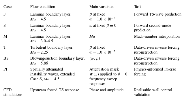


 μL2
 β
 ω=1.0×10⁻⁵
 Rey=1.12×10⁴
 (ω=1.0×10⁻⁵, β=2.2×10⁻⁴)
 L2

 Ma=4.5
 β=0
 μL2
 ω
 Rey=8.78×10³
 ω=3.1×10⁻⁴
 L2

 μL2
 Ma∈[3.0,4.5]
 ρu^
 Rey=7.52×10³
 Ma=3.50
 L2

 Ma=2.25
 ‖f^‖Ω
 β
 ω=1.0×10⁻⁵
 fρu
 Rey=5.29×10³
 (ω=1.0×10⁻⁵, β=1.92×10⁻⁴)
 L2
 fρu

 ‖f^‖Ω
 fρu
 Rey=4.07×10⁴
 (ω=4.6×10⁻⁵, β=4.0×10⁻⁵)
 L2
 fρu


 (ω=8.7×10⁻⁵)

 (ω=33×10−5)

 fρ
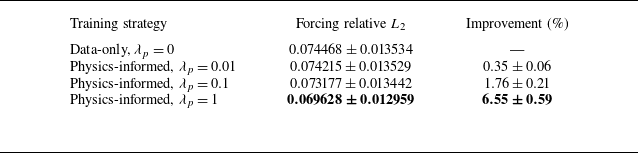


 Re(ρ^CFD)
 Re(q^natproj)
 Re(q^decay)

 ccal
 q^natclean=ccalq^TS
 W(x)
 W(x)
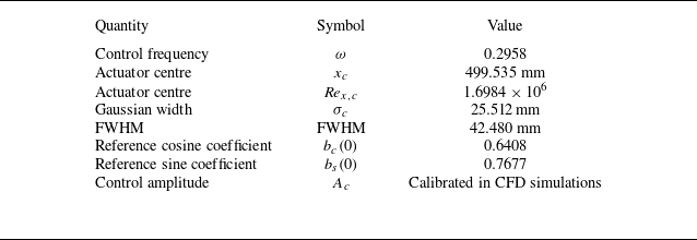

 xc
 σc

 Δϕ=π/2
 Ac=10−6
 xc
 xc±σc
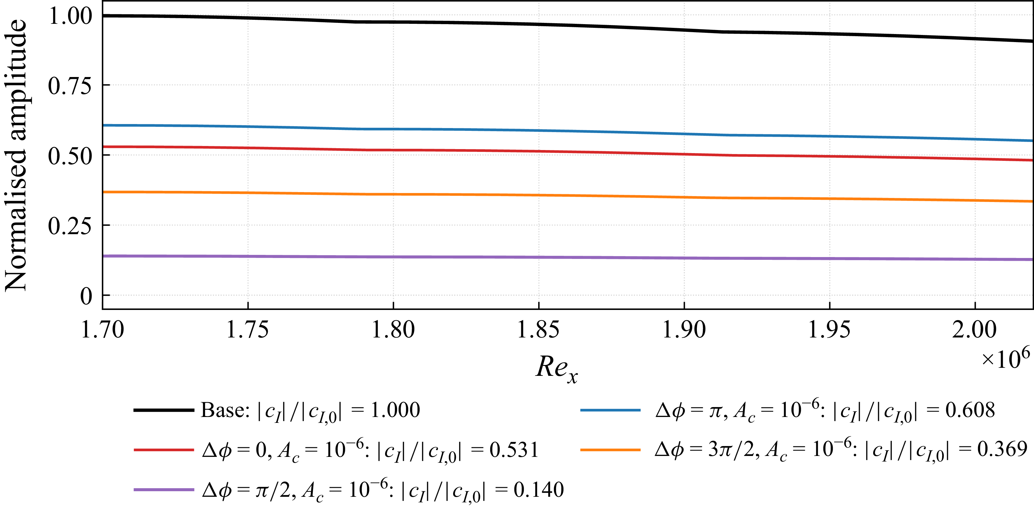
 Ac=10−6
 Rcoh=|cId,ctrl|/|cId,base|
 Δϕ=π/2
 14.0%
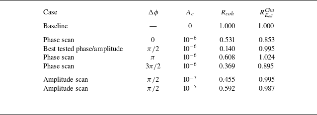
 Rcoh
 REallChu
 ΩE
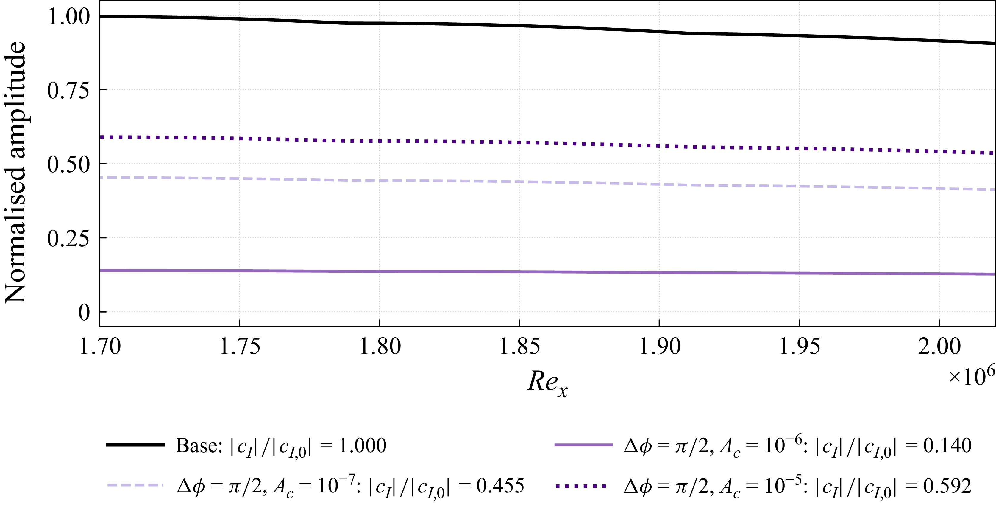
 Δϕ=π/2
 Ac=10−6

 Δϕ=π/2
 Ac=10−6
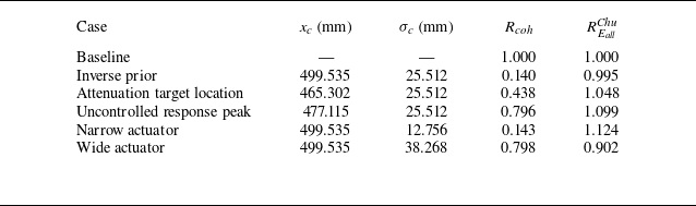
 Δϕ=π/2
 Ac=10−6
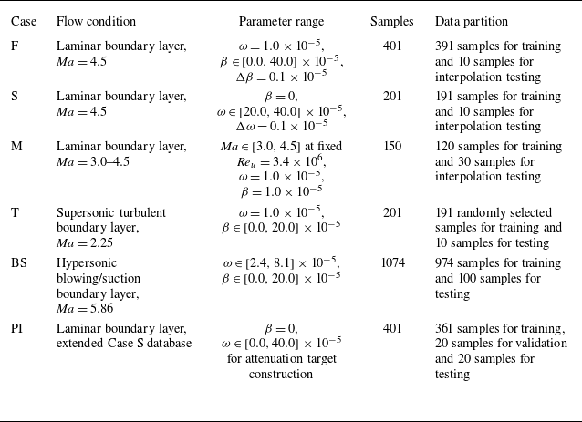
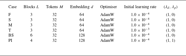

 L2

 L2