1 Introduction
Inverse cascade of energy is a well-known feature of two-dimensional homogeneous isotropic turbulence (HIT). It is generally understood as a consequence of the positive-definiteness of two ideally conserved quantities, energy and enstrophy, the enstrophy cascade being forward (Kraichnan Reference Kraichnan1967). In three-dimensional HIT, in addition to energy, the other quantity conserved in the inviscid limit is helicity (Moreau Reference Moreau1961; Moffatt Reference Moffatt1969), which is not positive-definite. Accordingly only forward cascades of both energy and helicity are expected (Brissaud et al. Reference Brissaud, Frisch, Leorat, Lesieur and Mazure1973; Chen, Chen & Eyink Reference Chen, Chen and Eyink2003a; Chen et al. Reference Chen, Chen, Eyink and Holm2003b; Mininni, Alexakis & Pouquet Reference Mininni, Alexakis and Pouquet2006; Alexakis Reference Alexakis2017). However, projecting the velocity field on a basis of homochiral modes, e.g. positive helical modes, helicity thus becomes positive-definite, and an inverse cascade of energy is expected together with a forward cascade of helicity. This has been shown numerically by solving a decimated model of the Navier–Stokes equations (NSE) in which the negative helical modes have been arbitrarily set to zero (Biferale, Musacchio & Toschi Reference Biferale, Musacchio and Toschi2012, Reference Biferale, Musacchio and Toschi2013). Limited to interactions among positive helical modes, the energy flux has been found to be negative at infrared scales, i.e. scales larger than the energy forcing scale, leading to an inverse cascade of energy.
Although such a homochiral framework is theoretically interesting, it is not yet clear whether it could be applied to the NSE that involve both homochiral and heterochiral triadic interactions. Kessar et al. (Reference Kessar, Plunian, Stepanov and Balarac2015) solved the NSE numerically, with energy injected at large scales and positive helicity injected over the entire inertial range of the energy cascade. The energy of the positive helical modes was found to be higher than the energy of the negative helical modes by several orders of magnitude, corresponding to a near-maximum helical state of turbulence. They found that the energy flux resulting from the positive helical mode interactions was indeed negative, as predicted by the homochiral phenomenology. However, the energy flux resulting from the heterochiral interactions was found to be positive and dominant, leading to a positive total energy flux, and therefore to a forward energy cascade. Finally, the energy spectrum was found to satisfy a power law close to  $k^{-7/3}$, related to the forward cascade of helicity in homochiral turbulence.
In Sahoo, Alexakis & Biferale (Reference Sahoo, Alexakis and Biferale2017), the nonlinear operator of the NSE has been modified in order to control the relative weight of homochiral to heterochiral triadic interactions. In the high-Reynolds-number limit, by increasing the weight of homochiral triadic interactions, they found a sharp transition from forward to inverse energy cascade at infrared scales. It remains to be seen whether such an inverse cascade can occur dynamically from the direct numerical simulation of the NSE, without any type of decimation, which is the subject of this paper.
We report results obtained from the direct simulation of the NSE, with positive helicity injected at all scales, as in Kessar et al. (Reference Kessar, Plunian, Stepanov and Balarac2015), but now including the scales larger than the energy forcing scale, namely the infrared scales. Although the flow is again not in an ideal state of maximum helicity because it contains both positive and negative helical modes interacting dynamically, an inverse cascade of energy is nevertheless found. This is the first evidence of inverse energy cascade in three-dimensional homogeneous isotropic turbulence, in a framework more general than that of homochiral triads.
2 Helical forcing
We solve the NSE
 $$\begin{eqnarray}\unicode[STIX]{x2202}_{t}\boldsymbol{u}=-(\boldsymbol{u}\boldsymbol{\cdot }\unicode[STIX]{x1D735})\boldsymbol{u}-\unicode[STIX]{x1D735}P+\unicode[STIX]{x1D708}\unicode[STIX]{x1D6FB}^{2}\boldsymbol{u}-\unicode[STIX]{x1D707}\unicode[STIX]{x1D6FB}^{-4}\boldsymbol{u}+\boldsymbol{f},\end{eqnarray}$$
where  $\boldsymbol{u}$ denotes the velocity field,
 $P$ the pressure normalized by the mass density,
 $\unicode[STIX]{x1D708}$ the fluid viscosity and
 $\boldsymbol{f}$ the flow forcing. We consider an incompressible fluid such that
 $\unicode[STIX]{x1D735}\boldsymbol{\cdot }\boldsymbol{u}=0$. We introduce the additional term
 $\unicode[STIX]{x1D707}\unicode[STIX]{x1D6FB}^{-4}\boldsymbol{u}$, which mimics large-scale friction in order to avoid large-scale energy accumulation in case an inverse cascade occurs.
In Fourier space, equation (2.1) becomes
 $$\begin{eqnarray}\unicode[STIX]{x2202}_{t}\boldsymbol{u}(\boldsymbol{k})=-{\mathcal{F}}[(\boldsymbol{u}\boldsymbol{\cdot }\unicode[STIX]{x1D735})\boldsymbol{u}](\boldsymbol{k})-\text{i}P(\boldsymbol{k})\boldsymbol{k}-(\unicode[STIX]{x1D708}k^{2}+\unicode[STIX]{x1D707}k^{-4})\boldsymbol{u}(\boldsymbol{k})+\boldsymbol{f}(\boldsymbol{k}),\end{eqnarray}$$
where  ${\mathcal{F}}[(\boldsymbol{u}\boldsymbol{\cdot }\unicode[STIX]{x1D735})\boldsymbol{u}](\boldsymbol{k})$ denotes the Fourier transform of the nonlinear term
 $(\boldsymbol{u}\boldsymbol{\cdot }\unicode[STIX]{x1D735})\boldsymbol{u}$, and
 $k=|\boldsymbol{k}|$. In (2.2)
 $\boldsymbol{u}(\boldsymbol{k})$,
 $P(\boldsymbol{k})$ and
 $\boldsymbol{f}(\boldsymbol{k})$ denote the Fourier coefficients of, respectively,
 $\boldsymbol{u}$,
 $P$ and
 $\boldsymbol{f}$ at wavenumber
 $\boldsymbol{k}$. The same notation will be used throughout the paper.
A crucial issue is to derive a forcing  $\boldsymbol{f}(\boldsymbol{k})$ such that helicity
 $H(\boldsymbol{k})=\frac{1}{2}\boldsymbol{u}(\boldsymbol{k})\boldsymbol{\cdot }\boldsymbol{w}(\boldsymbol{k})^{\ast }$, where
 $\boldsymbol{w}(\boldsymbol{k})=\text{i}\boldsymbol{k}\times \boldsymbol{u}(\boldsymbol{k})$ is the vorticity, can be injected independently from energy
 $E(\boldsymbol{k})=\frac{1}{2}\boldsymbol{u}(\boldsymbol{k})\boldsymbol{\cdot }\boldsymbol{u}(\boldsymbol{k})^{\ast }$. Therefore
 $\boldsymbol{f}(\boldsymbol{k})$ has to satisfy
 $$\begin{eqnarray}\displaystyle \boldsymbol{f}(\boldsymbol{k})\boldsymbol{\cdot }\boldsymbol{u}(\boldsymbol{k})^{\ast }=\unicode[STIX]{x1D700}_{E}(\boldsymbol{k}),\quad \boldsymbol{f}(\boldsymbol{k})\boldsymbol{\cdot }\boldsymbol{w}(\boldsymbol{k})^{\ast }=\unicode[STIX]{x1D700}_{H}(\boldsymbol{k}), & & \displaystyle\end{eqnarray}$$
where  $\unicode[STIX]{x1D700}_{E}(\boldsymbol{k})$ and
 $\unicode[STIX]{x1D700}_{H}(\boldsymbol{k})$ are the injection rates of, respectively, energy and helicity.
2.1 Helical mode decomposition
Each velocity Fourier coefficient is split into helical modes (Craya Reference Craya1958; Herring Reference Herring1974; Cambon & Jacquin Reference Cambon and Jacquin1989; Waleffe Reference Waleffe1992; Lessinnes et al. Reference Lessinnes, Plunian, Stepanov and Carati2011),
 $$\begin{eqnarray}\boldsymbol{u}(\boldsymbol{k})=u^{+}(\boldsymbol{k})\boldsymbol{h}^{+}(\boldsymbol{k})+u^{-}(\boldsymbol{k})\boldsymbol{h}^{-}(\boldsymbol{k})\equiv \boldsymbol{u}^{+}(\boldsymbol{k})+\boldsymbol{u}^{-}(\boldsymbol{k}),\end{eqnarray}$$
where  $u^{\pm }(\boldsymbol{k})$ are complex scalars and
 $\boldsymbol{h}^{\pm }(\boldsymbol{k})$ are the two eigenvectors of the curl operator, satisfying
 $\text{i}\boldsymbol{k}\times \boldsymbol{h}^{\pm }(\boldsymbol{k})=\pm k\boldsymbol{h}^{\pm }(\boldsymbol{k})$. The latter are defined as
 $$\begin{eqnarray}\boldsymbol{h}^{\pm }(\boldsymbol{k})=\frac{1}{\sqrt{2}}\frac{(\boldsymbol{z}_{\boldsymbol{k}}\times \boldsymbol{k})\times \boldsymbol{k}}{k|\boldsymbol{z}_{\boldsymbol{k}}\times \boldsymbol{k}|}\pm \frac{\text{i}}{\sqrt{2}}\frac{\boldsymbol{z}_{\boldsymbol{k}}\times \boldsymbol{k}}{|\boldsymbol{z}_{\boldsymbol{k}}\times \boldsymbol{k}|},\end{eqnarray}$$
where at each time step the vector  $\boldsymbol{z}_{\boldsymbol{k}}$ is generated randomly for each wavenumber
 $\boldsymbol{k}$, keeping
 $\boldsymbol{z}_{\boldsymbol{k}}\times \boldsymbol{k}\neq 0$ (Waleffe Reference Waleffe1992). Note that
 $\boldsymbol{h}^{+}(\boldsymbol{k})$ and
 $\boldsymbol{h}^{-}(\boldsymbol{k})$ are complex conjugate of each other,
 $\boldsymbol{h}^{\pm }(\boldsymbol{k})=\boldsymbol{h}^{\mp }(\boldsymbol{k})^{\ast }$. They are vectors of unit norm,
 $|\boldsymbol{h}^{\pm }(\boldsymbol{k})|^{2}=\boldsymbol{h}^{+}(\boldsymbol{k})\boldsymbol{\cdot }\boldsymbol{h}^{-}(\boldsymbol{k})=1$, and the scalar product of each of them with itself is equal to zero,
 $\boldsymbol{h}^{+}(\boldsymbol{k})\boldsymbol{\cdot }\boldsymbol{h}^{+}(\boldsymbol{k})=\boldsymbol{h}^{-}(\boldsymbol{k})\boldsymbol{\cdot }\boldsymbol{h}^{-}(\boldsymbol{k})=0$. Then the helical modes
 $u^{\pm }(\boldsymbol{k})$ can be derived from (2.4) according to
 $$\begin{eqnarray}u^{\pm }(\boldsymbol{k})=\boldsymbol{u}(\boldsymbol{k})\boldsymbol{\cdot }\boldsymbol{h}^{\mp }(\boldsymbol{k}).\end{eqnarray}$$
The vorticity can also be expressed in terms of helical modes,
 $$\begin{eqnarray}\boldsymbol{w}(\boldsymbol{k})=k(u^{+}(\boldsymbol{k})\boldsymbol{h}^{+}(\boldsymbol{k})-u^{-}(\boldsymbol{k})\boldsymbol{h}^{-}(\boldsymbol{k})).\end{eqnarray}$$
Then, the energy and helicity take the form
 $$\begin{eqnarray}\displaystyle E(\boldsymbol{k})=E^{+}(\boldsymbol{k})+E^{-}(\boldsymbol{k}),\quad H(\boldsymbol{k})=k(E^{+}(\boldsymbol{k})-E^{-}(\boldsymbol{k})), & & \displaystyle\end{eqnarray}$$
with  $E^{\pm }(\boldsymbol{k})=\frac{1}{2}|u^{\pm }(\boldsymbol{k})|^{2}$.
2.2 Dynamical forcing
Looking for a flow forcing of the form
 $$\begin{eqnarray}\boldsymbol{f}(\boldsymbol{k})=c^{+}(\boldsymbol{k})u^{+}(\boldsymbol{k})\boldsymbol{h}^{+}(\boldsymbol{k})+c^{-}(\boldsymbol{k})u^{-}(\boldsymbol{k})\boldsymbol{h}^{-}(\boldsymbol{k}),\end{eqnarray}$$
from (2.3), (2.4) and (2.7), we obtain
 $$\begin{eqnarray}c^{\pm }(\boldsymbol{k})=\frac{\unicode[STIX]{x1D700}_{E}(\boldsymbol{k})\pm \unicode[STIX]{x1D700}_{H}(\boldsymbol{k})/k}{4E^{\pm }(\boldsymbol{k})}.\end{eqnarray}$$
As our purpose is to study strongly helical turbulence, one type of helical mode, here  $\boldsymbol{u}^{-}(\boldsymbol{k})$, is expected to have a small energy
 $E^{-}(\boldsymbol{k})$, possibly leading to high values of
 $c^{-}(\boldsymbol{k})$. To avoid using a very small time step, which would be numerically intractable, we integrate analytically the equations
 $\unicode[STIX]{x2202}u^{\pm }(\boldsymbol{k},t)/\unicode[STIX]{x2202}t=c^{\pm }(\boldsymbol{k},t)u^{\pm }(\boldsymbol{k},t)$, leading to
 $$\begin{eqnarray}u_{0}^{\pm }(\boldsymbol{k},t+\unicode[STIX]{x0394}t)=\text{e}^{\text{i}\,arg\,u^{\pm }(\boldsymbol{k},t)}\left(\left[\unicode[STIX]{x1D700}_{E}(\boldsymbol{k},t)\pm \frac{\unicode[STIX]{x1D700}_{H}(\boldsymbol{k},t)}{k}\right]\unicode[STIX]{x0394}t+|u^{\pm }(\boldsymbol{k},t)|^{2}\right)^{1/2}.\end{eqnarray}$$
Then  $\boldsymbol{u}_{0}(\boldsymbol{k},t+\unicode[STIX]{x0394}t)=u_{0}^{+}(\boldsymbol{k},t+\unicode[STIX]{x0394}t)\boldsymbol{h}^{+}(\boldsymbol{k})+u_{0}^{-}(\boldsymbol{k},t+\unicode[STIX]{x0394}t)\boldsymbol{h}^{-}(\boldsymbol{k})$ is taken as an initial condition in the calculation of the NSE at time step
 $t+\unicode[STIX]{x0394}t$. To achieve the desired state of high helicity, we use the following asymptotic quenching:
 $$\begin{eqnarray}\unicode[STIX]{x1D700}_{H}(\boldsymbol{k},t)=\tilde{\unicode[STIX]{x1D700}}_{H}\left(1-\frac{|E^{+}(\boldsymbol{k},t)-E^{-}(\boldsymbol{k},t)|}{E^{+}(\boldsymbol{k},t)+E^{-}(\boldsymbol{k},t)}\right),\end{eqnarray}$$
where  $\tilde{\unicode[STIX]{x1D700}}_{H}$ is the strength of helicity injection rate.
3 Energy and helicity
3.1 Integral quantities
The simulations are performed with the pseudo-spectral code TARANG (Verma et al. Reference Verma, Chatterjee, Yadav, Paul, Chandra and Samtaney2013; Stepanov et al. Reference Stepanov, Teimurazov, Titov, Verma, Barman, Kumar and Plunian2018; Teimurazov et al. Reference Teimurazov, Stepanov, Verma, Barman, Kumar and Sadhukhan2018), in a triply periodic domain of size  $(2\unicode[STIX]{x03C0})^{3}$. Energy is injected at the permanent rate
 $\unicode[STIX]{x1D700}_{E}(\boldsymbol{k})=0.2$, over
 $|\boldsymbol{k}|=k_{E}\in ]\!9,10\!]$. The viscosity and large-scale friction values are taken as
 $\unicode[STIX]{x1D708}=1.5\times 10^{-3}$ and
 $\unicode[STIX]{x1D707}=5\times 10^{-2}$, for which a resolution of
 $512^{3}$ is sufficient. The simulations differ by the values chosen for
 $\tilde{\unicode[STIX]{x1D700}}_{H}$, which is applied over
 $|\boldsymbol{k}|=k_{H}\in [1,10^{2}]$. Some variations of the parameters
 $\unicode[STIX]{x1D708}$ and
 $k_{H}$ will be discussed in § 4.3.
Total energy  $E_{tot}$, total helicity
 $H_{tot}$, energy dissipation rates
 $D_{E}^{\unicode[STIX]{x1D708}},D_{E}^{\unicode[STIX]{x1D707}}$ and
 $D_{E}^{\unicode[STIX]{x1D708}}+D_{E}^{\unicode[STIX]{x1D707}}$, and helicity dissipation rates
 $D_{H}^{\unicode[STIX]{x1D708}},D_{H}^{\unicode[STIX]{x1D707}}$ and
 $D_{H}^{\unicode[STIX]{x1D708}}+D_{H}^{\unicode[STIX]{x1D707}}$, plotted versus time for
 $\unicode[STIX]{x1D700}_{E}=0.2$ and
 $\tilde{\unicode[STIX]{x1D700}}_{H}=25$. The time range
 $t\in [180,280]$ over which the statistics are calculated is indicated, for each curve, by a thicker line.

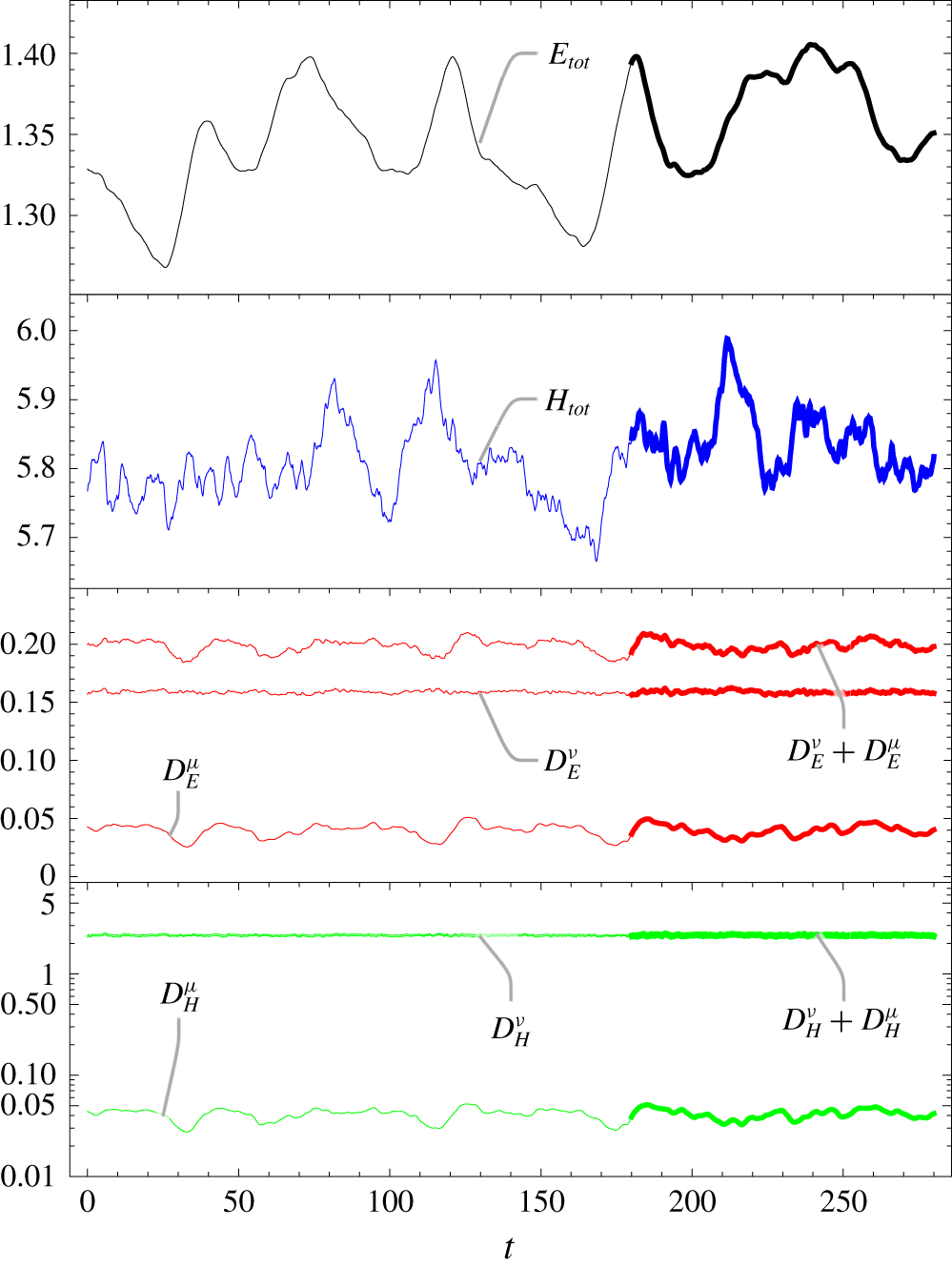
In figure 1, several integral quantities are plotted versus time for  $\tilde{\unicode[STIX]{x1D700}}_{H}=25$. We define
 $X_{tot}=\int X(\boldsymbol{k})\,\text{d}\boldsymbol{k}$, with
 $X=E$ for total energy and
 $X=H$ for total helicity. The molecular dissipation rate of
 $X$ is given by
 $D_{X}^{\unicode[STIX]{x1D708}}=2\unicode[STIX]{x1D708}\!\int \!k^{2}X(\boldsymbol{k})\,\text{d}\boldsymbol{k}$, and the friction dissipation rate by
 $D_{X}^{\unicode[STIX]{x1D707}}=2\unicode[STIX]{x1D707}\!\int \!k^{-4}X(\boldsymbol{k})\,\text{d}\boldsymbol{k}$. In figure 1 we see that
 $H_{tot}$ varies on a time scale much smaller than
 $E_{tot}$, suggesting a turbulence governed by helicity rather than energy. On average, we have
 $D_{E}^{\unicode[STIX]{x1D708}}+D_{E}^{\unicode[STIX]{x1D707}}=0.2$, which corresponds to the total injection rate of energy
 $\unicode[STIX]{x1D700}_{E}=\int \!\unicode[STIX]{x1D700}_{E}(\boldsymbol{k})\,\text{d}\boldsymbol{k}$. Both
 $D_{E}^{\unicode[STIX]{x1D707}}$ and
 $D_{H}^{\unicode[STIX]{x1D707}}$ are mostly identical. This is because friction is dominated by the largest scale
 $k=1$ where turbulence is close to maximum helicity, implying
 $H(k=1)\approx kE(k=1)$. In the rest of the paper, the spectra and fluxes are obtained by averaging over frames spread over 50 to 100 time units. For
 $\tilde{\unicode[STIX]{x1D700}}_{H}=25$, this time window is represented in figure 1 by the thick part of the curves.
An estimate of the Taylor-microscale Reynolds number,  $R_{\unicode[STIX]{x1D706}}=u^{\prime }\unicode[STIX]{x1D706}/\unicode[STIX]{x1D708}$, can be obtained with
 $u^{\prime }=\sqrt{2\bar{E}_{tot}/3}$ and
 $\unicode[STIX]{x1D706}=\sqrt{15\unicode[STIX]{x1D708}{u^{\prime }}^{2}/\unicode[STIX]{x1D700}_{E}}$ (Pope Reference Pope2000). From figure 1 the mean kinetic energy is
 $\bar{E}_{tot}\approx 1.35$, which gives
 $u^{\prime }\approx 0.95$ and
 $\unicode[STIX]{x1D706}\approx 0.32$, thus leading to
 $R_{\unicode[STIX]{x1D706}}\approx 200$, which compares well with other numerical simulations of the same resolution (Okamoto et al. Reference Okamoto, Yoshimatsu, Schneider, Farge and Kaneda2007).
3.2 Energy and helicity spectra and fluxes
Taking the dot product of (2.2) with  $\boldsymbol{x}(\boldsymbol{k})^{\ast }$, we obtain the equations for modal energy and helicity,
 $$\begin{eqnarray}\displaystyle \unicode[STIX]{x2202}_{t}X(\boldsymbol{k}) & = & \displaystyle -\text{Re}\{\boldsymbol{x}(\boldsymbol{k})^{\ast }\boldsymbol{\cdot }{\mathcal{F}}[(\boldsymbol{u}\boldsymbol{\cdot }\unicode[STIX]{x1D735})\boldsymbol{u}](\boldsymbol{k})\}\nonumber\\ \displaystyle & & \displaystyle -\,2(\unicode[STIX]{x1D708}k^{2}+\unicode[STIX]{x1D707}k^{-4})X(\boldsymbol{k})+\unicode[STIX]{x1D700}_{X}(\boldsymbol{k}),\end{eqnarray}$$
where  $(X,\boldsymbol{x})=(E,\boldsymbol{u})$ or
 $(X,\boldsymbol{x})=(H,\boldsymbol{w})$,
 ${\mathcal{F}}$ standing for Fourier transform, and
 $\unicode[STIX]{x1D700}_{X}(\boldsymbol{k})$ satisfying (2.3). Rewriting (3.1) for
 $\boldsymbol{k}^{\prime }$, and taking the sum over
 $\boldsymbol{k}^{\prime }$ such that
 $k<|\boldsymbol{k}^{\prime }|\leqslant k+\text{d}k$ (Verma Reference Verma2019), leads to
 $$\begin{eqnarray}\unicode[STIX]{x2202}_{t}X(k)=-\unicode[STIX]{x2202}_{k}\unicode[STIX]{x1D6F1}_{X}(k)-D_{X}(k)+\unicode[STIX]{x1D700}_{X}(k),\end{eqnarray}$$
with
 $$\begin{eqnarray}\displaystyle & \displaystyle X(k)\,\text{d}k=\mathop{\sum }_{k<|\boldsymbol{k}^{\prime }|\leqslant k+\text{d}k}X(\boldsymbol{k}^{\prime }), & \displaystyle\end{eqnarray}$$
 $$\begin{eqnarray}\displaystyle & \displaystyle \unicode[STIX]{x1D6F1}_{X}(k)=\mathop{\sum }_{|\boldsymbol{k}^{\prime }|\leqslant k}\text{Re}\{\boldsymbol{x}(\boldsymbol{k}^{\prime })^{\ast }\boldsymbol{\cdot }{\mathcal{F}}[(\boldsymbol{u}\boldsymbol{\cdot }\unicode[STIX]{x1D735})\boldsymbol{u}](\boldsymbol{k}^{\prime })\}, & \displaystyle\end{eqnarray}$$
 $$\begin{eqnarray}\displaystyle & \displaystyle D_{X}(k)\,\text{d}k=\mathop{\sum }_{k<|\boldsymbol{k}^{\prime }|\leqslant k+\text{d}k}2(\unicode[STIX]{x1D708}{k^{\prime }}^{2}+\unicode[STIX]{x1D707}{k^{\prime }}^{-4})X(\boldsymbol{k}^{\prime }), & \displaystyle\end{eqnarray}$$
 $$\begin{eqnarray}\displaystyle & \displaystyle \unicode[STIX]{x1D700}_{X}(k)\,\text{d}k=\mathop{\sum }_{k<|\boldsymbol{k}^{\prime }|\leqslant k+\text{d}k}\unicode[STIX]{x1D700}_{X}(\boldsymbol{k}^{\prime }). & \displaystyle\end{eqnarray}$$
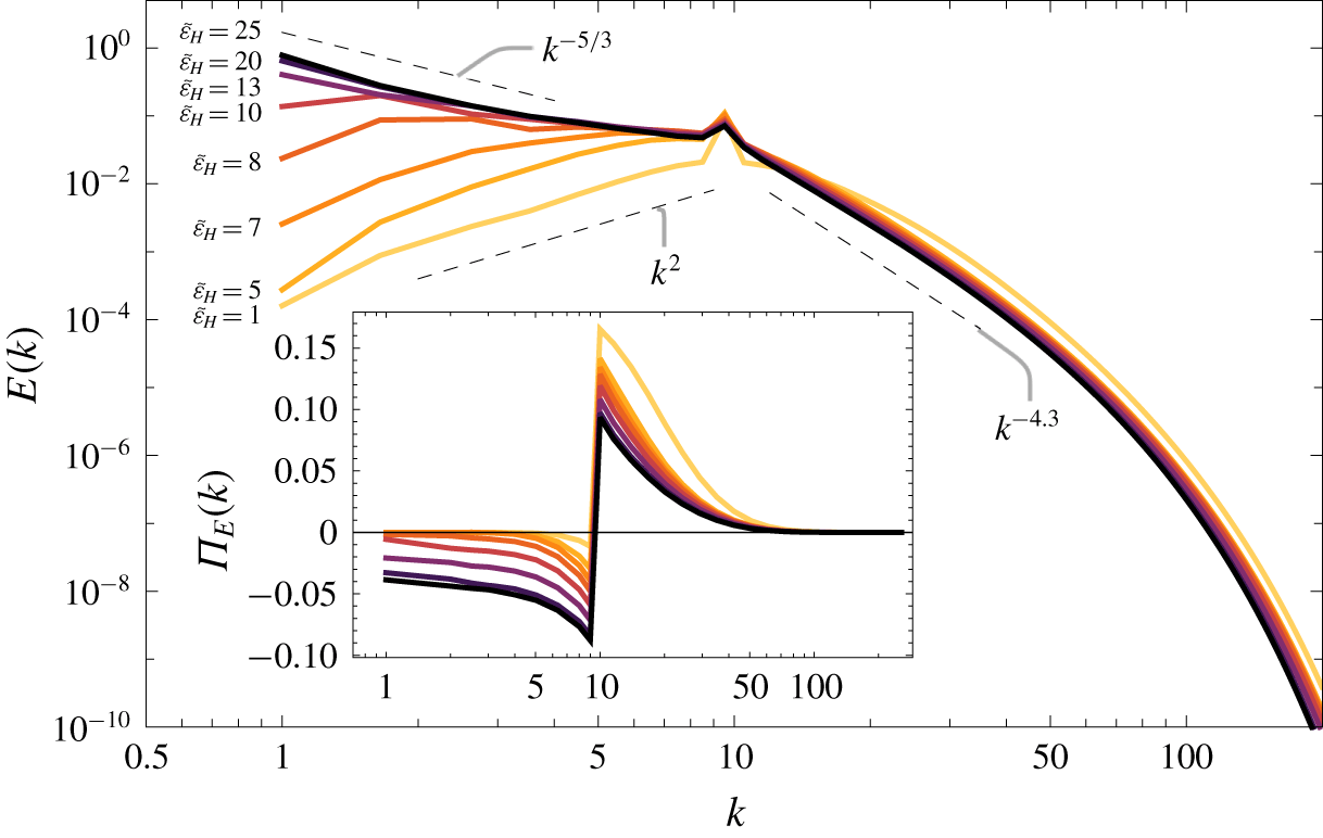
The energy spectral density  $E(k)$ and flux
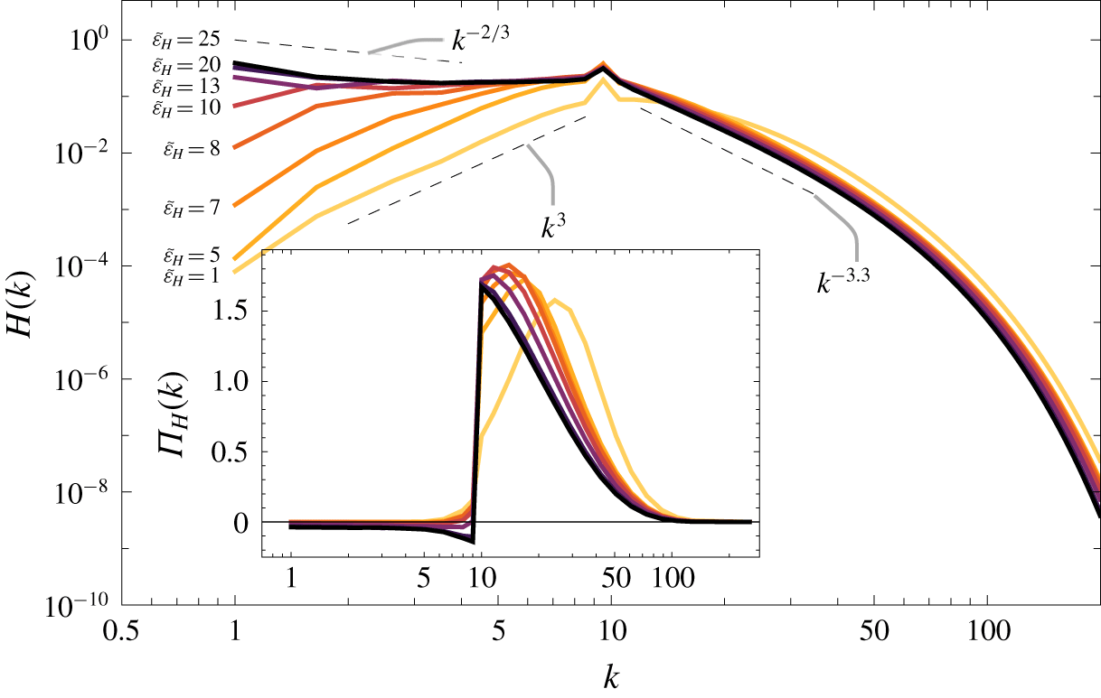
 $\unicode[STIX]{x1D6F1}_{E}(k)$ in figure 2, and the helicity spectral density
 $H(k)$ and flux
 $\unicode[STIX]{x1D6F1}_{H}(k)$ in figure 3, are plotted for
 $\tilde{\unicode[STIX]{x1D700}}_{H}\in S$, with
 $S=\{1;5;7;8;10;13;20;25\}$. For
 $\tilde{\unicode[STIX]{x1D700}}_{H}=1$, the fluxes of energy and helicity are non-zero only for
 $k\geqslant 10$. As both fluxes are positive, they correspond to forward cascades of energy and helicity, as expected in three-dimensional turbulence. In figure 3, the shape of the helicity flux obtained for
 $\tilde{\unicode[STIX]{x1D700}}_{H}=1$, with a maximum at
 $k\approx 20$, is similar to the one obtained by Kessar et al. (Reference Kessar, Plunian, Stepanov and Balarac2015) in which helicity was injected only at scales smaller than the energy injection scale.
With the increase of  $\tilde{\unicode[STIX]{x1D700}}_{H}$ from 1 to 25, the energy flux is shifted downwards. It then becomes negative in the infrared domain
 $k\leqslant 9$, leading to an inverse cascade of energy. With the increase of
 $\tilde{\unicode[STIX]{x1D700}}_{H}$, the scale at which the helicity flux is maximum is also shifted, towards the energy injection scale. For
 $k\geqslant 10$ the helicity flux is positive, corresponding to a forward cascade of helicity. Such a dual cascade is consistent with the homochiral phenomenology. For
 $\tilde{\unicode[STIX]{x1D700}}_{H}=25$, in the infrared domain
 $k\leqslant 9$, the energy spectrum obeys a
 $k^{-5/3}$ scaling law. For
 $k\geqslant 10$ the energy spectral slope is approximately
 $E(k)\propto k^{-4.3}$, which is steeper than the
 $E(k)\propto k^{-7/3}$ predicted by the homochiral phenomenology. Most probably this is due to the fact that, at scales smaller than the energy injection scales, the viscous dissipation cannot be neglected, implying that an inertial range can hardly be identified.
Energy spectra and fluxes (inset). The energy injection rate  $\unicode[STIX]{x1D700}_{E}=0.2$ is applied at
 $k_{E}\in ]\!9,10\!]$. The helicity injection rate
 $\tilde{\unicode[STIX]{x1D700}}_{H}\in \{1;5;7;8;10;13;20;25\}$ is applied at
 $k_{H}\in [1,10^{2}]$.

Helicity spectra and fluxes (inset) for the same parameters as in figure 2.

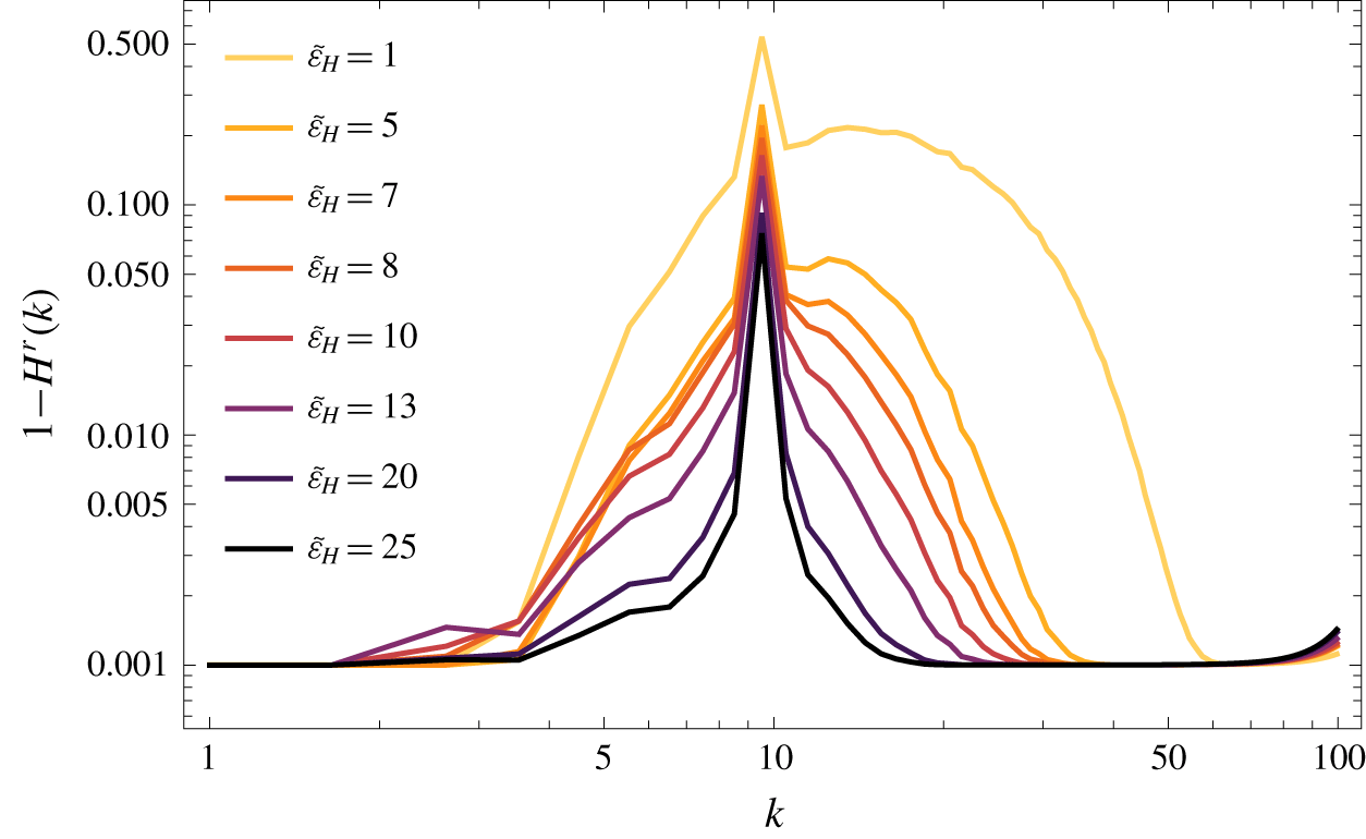
Deviation to maximum chirality,  $1-H^{r}(k)$, for the same parameters as in figure 2.

A measure of chirality is given by the relative helicity  $H^{r}(k)=H(k)/kE(k)$, which satisfies the realizability condition
 $0\leqslant |H^{r}(k)|\leqslant 1$. A non-helical turbulence corresponds to
 $|H^{r}(k)|=0$. A maximum helical turbulence corresponds to
 $|H^{r}(k)|=1$, which can be obtained only in the homochiral framework. In figure 4,
 $1-H^{r}(k)$ is plotted for
 $\tilde{\unicode[STIX]{x1D700}}_{H}\in S$. We find that increasing
 $\tilde{\unicode[STIX]{x1D700}}_{H}$ leads to lower values of
 $1-H^{r}(k)$ in broader ranges of scales. The turbulent state is then closer to maximum chirality. We note that the lower bound of
 $10^{-3}$ for
 $1-H^{r}(k)$ is prescribed by a restriction on
 $\unicode[STIX]{x1D700}_{H}$ in order to avoid a negative value under the square root in (2.11).
4 Helical modes
4.1 Energy fluxes
The energy equation for each helical mode is obtained by taking the real part of the dot product of (2.2) with  $\boldsymbol{u}^{\pm }(\boldsymbol{k})^{\ast }$. Then the energy equation is given by (3.1) with
 $(X,\boldsymbol{x})=(E^{\pm },\boldsymbol{u}^{\pm })$ and
 $2\unicode[STIX]{x1D700}_{E^{\pm }}(\boldsymbol{k})=\unicode[STIX]{x1D700}_{E}(\boldsymbol{k})\pm \unicode[STIX]{x1D700}_{H}(\boldsymbol{k})/k$. The equation satisfied by the energy spectral density of each helical mode is given by (3.2) with (3.3)–(3.6). Of course, the flux of total energy satisfies
 $$\begin{eqnarray}\unicode[STIX]{x1D6F1}_{E}(k)=\unicode[STIX]{x1D6F1}_{E^{+}}(k)+\unicode[STIX]{x1D6F1}_{E^{-}}(k).\end{eqnarray}$$
In addition, each flux  $\unicode[STIX]{x1D6F1}_{E^{\pm }}(k)$ can be decomposed into
 $$\begin{eqnarray}\displaystyle & \displaystyle \unicode[STIX]{x1D6F1}_{E^{+}}(k)=\unicode[STIX]{x1D6F1}_{+}^{+<}(k)+\unicode[STIX]{x1D6F1}_{-}^{+<}(k), & \displaystyle\end{eqnarray}$$
 $$\begin{eqnarray}\displaystyle & \displaystyle \unicode[STIX]{x1D6F1}_{E^{-}}(k)=\unicode[STIX]{x1D6F1}_{+}^{-<}(k)+\unicode[STIX]{x1D6F1}_{-}^{-<}(k), & \displaystyle\end{eqnarray}$$
where  $\unicode[STIX]{x1D6F1}_{b}^{a<}(k)$, with
 $a,b\equiv \pm$, denotes the energy flux from
 $\boldsymbol{u}^{a<}(\boldsymbol{k})$, meaning that
 $\boldsymbol{u}^{a}(\boldsymbol{k})$ is taken at wavenumbers inside a sphere of radius
 $k$ (the
 $k$-sphere), to
 $\boldsymbol{u}^{b}(\boldsymbol{k})$ taken at all wavenumbers. It is defined by
 $$\begin{eqnarray}\unicode[STIX]{x1D6F1}_{b}^{a<}(k)=\mathop{\sum }_{|\boldsymbol{k}^{\prime }|\leqslant k}\text{Re}\{\boldsymbol{u}^{a}(\boldsymbol{k}^{\prime })^{\ast }\boldsymbol{\cdot }{\mathcal{F}}[(\boldsymbol{u}\boldsymbol{\cdot }\unicode[STIX]{x1D735})\boldsymbol{u}^{b}](\boldsymbol{k}^{\prime })\},\end{eqnarray}$$
where  $\boldsymbol{u}^{b}={\mathcal{F}}^{-1}[\boldsymbol{u}^{b}(\boldsymbol{k})]$ is the inverse Fourier transform of
 $\boldsymbol{u}^{b}(\boldsymbol{k})$ (Verma Reference Verma2004; Kessar et al. Reference Kessar, Plunian, Stepanov and Balarac2015; Plunian, Stepanov & Verma Reference Plunian, Stepanov and Verma2019; Sadhukhan et al. Reference Sadhukhan, Samuel, Plunian, Stepanov, Samtaney and Verma2019). We can further decompose
 $\unicode[STIX]{x1D6F1}_{+}^{+<}(k)$ as
 $\unicode[STIX]{x1D6F1}_{+}^{+<}(k)=\unicode[STIX]{x1D6F1}_{+<}^{+<}(k)+\unicode[STIX]{x1D6F1}_{+>}^{+<}(k)$, where
 $\unicode[STIX]{x1D6F1}_{+<}^{+<}(k)$ denotes the energy flux from
 $\boldsymbol{u}^{+<}$ to
 $\boldsymbol{u}^{+<}$, and
 $\unicode[STIX]{x1D6F1}_{+>}^{+<}(k)$ the energy flux from
 $\boldsymbol{u}^{+<}$ to
 $\boldsymbol{u}^{+>}$. Here, again,
 $\boldsymbol{u}^{+<}$ and
 $\boldsymbol{u}^{+>}$ denote
 $\boldsymbol{u}^{+}(\boldsymbol{k})$ taken at wavenumbers, respectively, inside and outside the
 $k$-sphere (similar notation applies to
 $\boldsymbol{u}^{-<}$ and
 $\boldsymbol{u}^{->}$). By definition
 $\unicode[STIX]{x1D6F1}_{+<}^{+<}(k)=0$, implying that
 $\unicode[STIX]{x1D6F1}_{+}^{+<}(k)=\unicode[STIX]{x1D6F1}_{+>}^{+<}(k)$ (similarly
 $\unicode[STIX]{x1D6F1}_{-<}^{-<}(k)=0$ implies
 $\unicode[STIX]{x1D6F1}_{-}^{-<}(k)=\unicode[STIX]{x1D6F1}_{->}^{-<}(k)$).
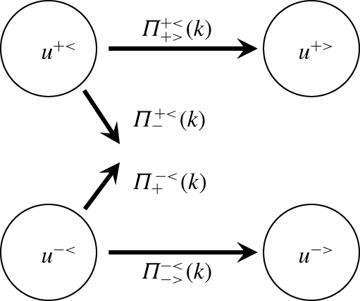
An illustration of the four fluxes  $\unicode[STIX]{x1D6F1}_{+}^{+<}(k),\unicode[STIX]{x1D6F1}_{-}^{+<}(k),\unicode[STIX]{x1D6F1}_{+}^{-<}(k)$ and
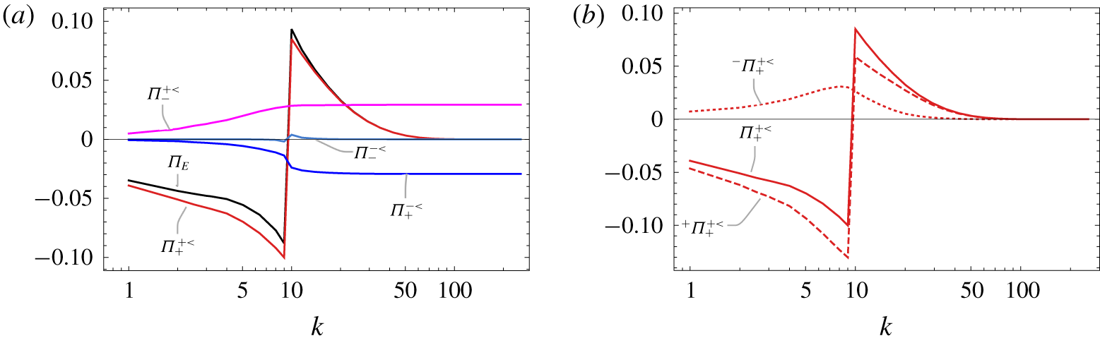
 $\unicode[STIX]{x1D6F1}_{-}^{-<}(k)$ is given in figure 5. They are plotted in figure 6(a) for
 $\tilde{\unicode[STIX]{x1D700}}_{H}=25$, together with
 $\unicode[STIX]{x1D6F1}_{E}(k)$, which is equal to the sum of the four. In the infrared domain
 $k\in [1,9]$,
 $\unicode[STIX]{x1D6F1}_{+}^{+<}(k)$ is clearly negative and close to
 $\unicode[STIX]{x1D6F1}_{E}(k)$, suggesting that it is mostly this flux that is responsible for the inverse energy cascade.
Illustration of the fluxes among helical modes. The notation  $\boldsymbol{u}^{\pm <}$ and
 $\boldsymbol{u}^{\pm >}$ corresponds to
 $\boldsymbol{u}^{\pm }(\boldsymbol{k})$ taken at wavenumbers, respectively, inside and outside the
 $k$-sphere. The non-horizontal arrows denote energy fluxes from one helical mode taken inside the
 $k$-sphere towards the opposite helical mode taken at all scales.

Helical mode fluxes for  $\unicode[STIX]{x1D700}_{E}=0.2$ and
 $\tilde{\unicode[STIX]{x1D700}}_{H}=25$. In (a), the four fluxes
 $\unicode[STIX]{x1D6F1}_{+}^{+<}(k),\unicode[STIX]{x1D6F1}_{-}^{+<}(k),\unicode[STIX]{x1D6F1}_{+}^{-<}(k)$ and
 $\unicode[STIX]{x1D6F1}_{-}^{-<}(k)$, illustrated in figure 5, are plotted together with the total energy flux
 $\unicode[STIX]{x1D6F1}_{E}(k)$ already plotted in figure 2. In (b), the flux
 $\unicode[STIX]{x1D6F1}_{+}^{+<}(k)$ is split into the homochiral flux
 $^{+}\unicode[STIX]{x1D6F1}_{+}^{+<}(k)$ and the heterochiral flux
 $^{-}\unicode[STIX]{x1D6F1}_{+}^{+<}(k)$.

It is thus interesting to further decompose the flux  $\unicode[STIX]{x1D6F1}_{+}^{+<}(k)$ as
 $\unicode[STIX]{x1D6F1}_{+}^{+<}(k)=^{+}\unicode[STIX]{x1D6F1}_{+}^{+<}(k)+^{-}\unicode[STIX]{x1D6F1}_{+}^{+<}(k)$ with
 $$\begin{eqnarray}\displaystyle \text{}^{\pm }\unicode[STIX]{x1D6F1}_{+}^{+<}(k)=\mathop{\sum }_{|\boldsymbol{k}^{\prime }|\leqslant k}\text{Re}\{\boldsymbol{u}^{+}(\boldsymbol{k}^{\prime })^{\ast }\boldsymbol{\cdot }{\mathcal{F}}[(\boldsymbol{u}^{\pm }\boldsymbol{\cdot }\unicode[STIX]{x1D735})\boldsymbol{u}^{+}](\boldsymbol{k}^{\prime })\}, & & \displaystyle\end{eqnarray}$$
where  $^{\pm }\unicode[STIX]{x1D6F1}_{+}^{+<}(k)$ is interpreted as the energy flux from
 $\boldsymbol{u}^{+<}$ to
 $\boldsymbol{u}^{+}$, with
 $\boldsymbol{u}^{\pm }$ acting as a mediator.
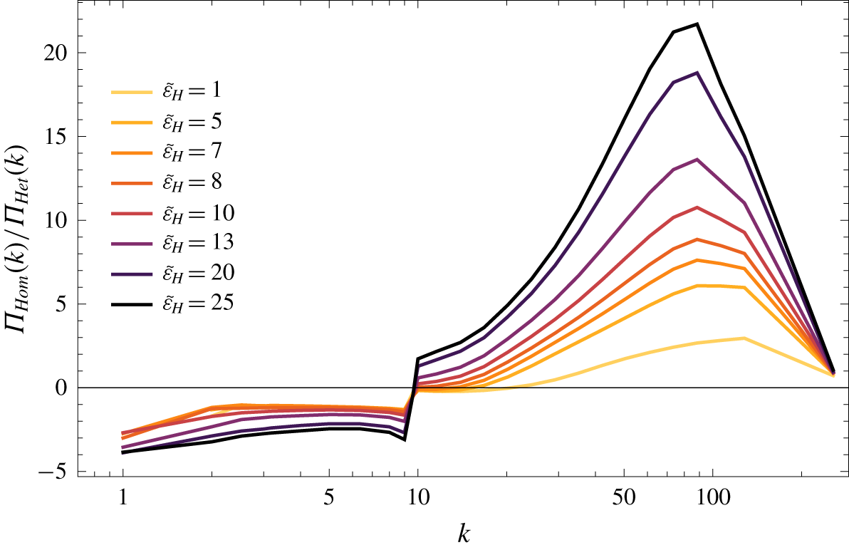
Ratio of the energy flux due to homochiral triads to the energy flux due to heterochiral triads, versus  $k$ and for the same parameters as in figure 2.

The three fluxes  $\unicode[STIX]{x1D6F1}_{+}^{+<}(k),^{+}\unicode[STIX]{x1D6F1}_{+}^{+<}(k)$ and
 $^{-}\unicode[STIX]{x1D6F1}_{+}^{+<}(k)$ are plotted in figure 6(b). In the infrared domain
 $k\in [1,9]$,
 $^{+}\unicode[STIX]{x1D6F1}_{+}^{+<}(k)\leqslant 0$ and
 $^{-}\unicode[STIX]{x1D6F1}_{+}^{+<}(k)\geqslant 0$, suggesting that the homochiral triadic interactions
 $(+,+,+)$ are mostly responsible for the inverse energy cascade. At scales smaller than the energy injection scales,
 $k\geqslant 10$, we observe that
 $^{+}\unicode[STIX]{x1D6F1}_{+}^{+<}(k)\geqslant 0$, which is in striking difference with previous simulations in which energy was injected at large scales (Kessar et al. Reference Kessar, Plunian, Stepanov and Balarac2015). In addition
 $|^{+}\unicode[STIX]{x1D6F1}_{+}^{+<}(k)|\geqslant |^{-}\unicode[STIX]{x1D6F1}_{+}^{+<}(k)|$, which contradicts the assumptions of the phenomenological model by Stepanov et al. (Reference Stepanov, Golbraikh, Frick and Shestakov2015).
From figure 2 we observe that the inverse cascade is continuously greater for increasing values of  $\tilde{\unicode[STIX]{x1D700}}_{H}$. This is in contrast with Sahoo et al. (Reference Sahoo, Alexakis and Biferale2017) in which a sharp transition between the cases with and without inverse cascade is reported. There are at least two main reasons to explain this discrepancy. First, in Sahoo et al. (Reference Sahoo, Alexakis and Biferale2017) such a sharp transition is only expected within the limit of high Reynolds numbers, which we are not studying here. Second, in Sahoo et al. (Reference Sahoo, Alexakis and Biferale2017), the ratio of heterochiral to homochiral triadic interactions is imposed, and it is imposed in the same way at all scales. This was done by solving a modified version of the NSE including a prescribed weighting between the homochiral and heterochiral nonlinear terms. Here, as we solve the NSE (2.2), the importance of homochiral versus heterochiral triadic interactions is not prescribed, and remains scale-dependent.
To contrast the strengths of heterochiral and homochiral triadic interactions, we calculate the ratio of their energy fluxes, which is given by
 $$\begin{eqnarray}\frac{\unicode[STIX]{x1D6F1}_{Hom}(k)}{\unicode[STIX]{x1D6F1}_{Het}(k)}=\frac{\text{}^{+}\unicode[STIX]{x1D6F1}_{+>}^{+<}(k)+^{-}\unicode[STIX]{x1D6F1}_{->}^{-<}(k)}{\unicode[STIX]{x1D6F1}_{E}(k)-(\text{}^{+}\unicode[STIX]{x1D6F1}_{+>}^{+<}(k)+^{-}\unicode[STIX]{x1D6F1}_{->}^{-<}(k))}.\end{eqnarray}$$
In figure 7, this ratio is plotted versus  $k$, for
 $\tilde{\unicode[STIX]{x1D700}}_{H}\in S$. This ratio is negative at scales larger than the energy injection scales, and positive at scales smaller than the energy injection scales. This is in agreement with the dual inverse energy cascade at large scales and forward helicity cascade at small scales. It is also clearly
 $k$-dependent. Finally, with the increase of
 $\tilde{\unicode[STIX]{x1D700}}_{H}$, the ratio
 $|\unicode[STIX]{x1D6F1}_{Hom}(k)|/|\unicode[STIX]{x1D6F1}_{Het}(k)|$ increases without sharp transition.
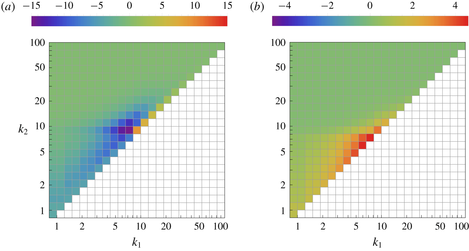
In  $(k_{1},k_{2})$ maps, two representations of fluxes from a
 $k_{1}$ inner sphere to a
 $k_{2}$ outer sphere
 $\unicode[STIX]{x1D6F1}_{{>}k_{2}}^{{<}k_{1}}$, for
 $\unicode[STIX]{x1D700}_{E}=0.2$ and
 $\tilde{\unicode[STIX]{x1D700}}_{H}=25$. In (a) the fluxes are calculated among positive homochiral triads only. In (b) the fluxes are calculated among all other triads, namely heterochiral and negative homochiral. The range of values taken by the fluxes is
 $[-15;15]$ in (a) and
 $[-5;5]$ in (b).

4.2 Non-local energy transfers
In order to investigate the degree of locality of the cascades, we further introduce the energy flux from an inner sphere of radius  $k_{1}$ to an outer sphere or radius
 $k_{2}$, which is defined as
 $$\begin{eqnarray}\unicode[STIX]{x1D6F1}_{{>}k_{2}}^{{<}k_{1}}=\mathop{\sum }_{|\boldsymbol{k}^{\prime }|\geqslant k_{2}}\text{Re}\{\boldsymbol{u}(\boldsymbol{k}^{\prime })^{\ast }\boldsymbol{\cdot }{\mathcal{F}}[(\boldsymbol{u}\boldsymbol{\cdot }\unicode[STIX]{x1D735})\boldsymbol{u}^{{<}k_{1}}](\boldsymbol{k}^{\prime })\},\end{eqnarray}$$
with
 $$\begin{eqnarray}\boldsymbol{u}^{{<}k_{1}}=\mathop{\sum }_{|\boldsymbol{k}^{\prime }|\leqslant k_{1}}{\mathcal{F}}^{-1}[\boldsymbol{u}(\boldsymbol{k}^{\prime })]\end{eqnarray}$$
and  $k_{1}\leqslant k_{2}$. For
 $k_{1}=k_{2}=k$ the two spheres are adjacent, implying that
 $\unicode[STIX]{x1D6F1}_{{>}k}^{{<}k}=\unicode[STIX]{x1D6F1}_{E}(k)$. Increasing the value of
 $k_{2}-k_{1}$ corresponds to moving the two spheres apart, and then to investigate non-local fluxes.
In figure 8, two  $(k_{1},k_{2})$ maps of
 $\unicode[STIX]{x1D6F1}_{{>}k_{2}}^{{<}k_{1}}$ are given, figure 8(a) giving the flux among positive homochiral triads, figure 8(b) giving the flux among all other triads (heterochiral and negative homochiral). In figure 8(a) the diagonal coincides with the flux
 $^{+}\unicode[STIX]{x1D6F1}_{+}^{+<}(k)$ represented in figure 6(b). In figure 8(b) the diagonal coincides with
 $\unicode[STIX]{x1D6F1}_{E}(k)-^{+}\unicode[STIX]{x1D6F1}_{+}^{+<}(k)$. In both cases the further away from the diagonal, the more non-local the fluxes are. In figure 8(a) the fluxes are mostly negative, with a minimum at
 $(k_{1},k_{2})\approx (7,9)$. This shows that the energy cascade is inverse, and due to weakly non-local interactions. In figure 8(b) the fluxes are positive and maximum on the diagonal, implying a forward cascade due to local interactions. In figure 8(b) the fluxes are approximately three times smaller than in figure 8(a), implying that the sum of both is qualitatively similar to figure 8(a). Therefore the inverse cascade obtained in the infrared domain is mainly due to weakly non-local interactions among positive homochiral triads
 $(+,+,+)$. The sum of the other triadic interactions leads to forward cascade, mainly local. The aforementioned non-local interactions leading to inverse energy cascade are also observed in two-dimensional hydrodynamic turbulence (Gupta et al. Reference Gupta, Jayaraman, Chatterjee, Sadhukhan, Samtaney and Verma2019; Verma Reference Verma2019).
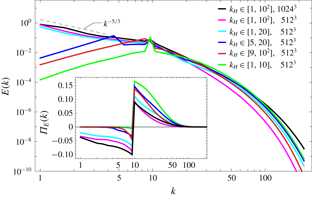
Energy spectra and fluxes (inset). The energy injection rate  $\unicode[STIX]{x1D700}_{E}=0.2$ is applied at
 $k_{E}\in ]\!9,10\!]$. From bottom to top of the energy spectra, the helicity injection rate
 $\tilde{\unicode[STIX]{x1D700}}_{H}=25$ is applied at
 $k_{H}\in [1,10]$,
 $]\!9,10^{2}\! ]$,
 $]\!5,20\!]$,
 $[1,20]$,
 $[1,10^{2}]$ and
 $[1,10^{2}]$ again. For the last curve the viscosity is twice as small and the resolution is equal to
 $1024^{3}$.

4.3 Varying the helicity injection range of scales
In contrast to previous studies (Biferale et al. Reference Biferale, Musacchio and Toschi2012, Reference Biferale, Musacchio and Toschi2013; Sahoo et al. Reference Sahoo, Alexakis and Biferale2017), here we can vary the range of scales in which helicity is injected. We already know that injecting helicity at scales smaller than the energy injection scales leads to a forward cascade of energy (Kessar et al. Reference Kessar, Plunian, Stepanov and Balarac2015). Here this would correspond to injecting helicity in the range  $k_{H}\in ]\!9,10^{2}\! ]$. From § 3.2, we also know that injecting helicity in the range
 $k_{H}\in [1,10^{2}]$ leads to an inverse energy cascade at large scales.
We now investigate additional cases injecting helicity in different scale ranges,  $k_{H}\in [1,20]$,
 $]\!5,20\!]$ and
 $[1,10]$, keeping all other parameters the same. The results of these three cases are plotted in figure 9, together with the case
 $k_{H}\in [1,10^{2}]$, already shown in figure 2, and the case
 $k_{H}\in ]\!9,10^{2}\! ]$.
The inverse cascade is obtained for  $k_{H}\in [1,20]$ but not for
 $k_{H}\in [1,10]$, suggesting that a sufficiently broad range of scales smaller than the energy injection scales is necessary to produce the inverse cascade. This emphasizes the role of non-local transfers identified in § 4.2. For
 $k_{H}\in ]\!5,20\!]$ the energy flux is negative for
 $k\in ]\!5,10\!]$ with an inverse cascade limited to these scales. This emphasizes the role of helicity injection at scales larger than the energy injection scale, i.e. the inverse energy cascade stops at scales where helicity is not injected. In summary, to obtain an inverse cascade it is necessary to inject helicity in a sufficiently broad range of scales on both sides of the energy injection range of scales.
Finally, the case  $k_{H}\in [1,10^{2}]$ with a twice smaller viscosity
 $\unicode[STIX]{x1D708}=0.75\times 10^{-3}$ and a resolution
 $1024^{3}$ is also plotted in figure 9. It corresponds to a mean kinetic energy
 $\bar{E}_{tot}\approx 2.1$, thus leading to
 $\unicode[STIX]{x1D706}\approx 0.28$, and a Taylor-microscale Reynolds number
 $R_{\unicode[STIX]{x1D706}}\approx 440$. The energy spectrum and flux are qualitatively similar to the case shown in figure 2, with again an inverse energy cascade at large scales.
5 Conclusions
The mechanism responsible for the inverse cascade of energy obtained at infrared scales agrees well with the homochiral framework described by Biferale et al. (Reference Biferale, Musacchio and Toschi2012). In order to generate a strongly helical turbulence, a positive helicity is injected at all scales, including the infrared scales. We observe a gradual amplification of the inverse cascade with the increase of helicity injection, reaching some saturation at a sufficiently large level of helicity injection. The negative energy flux is due to weakly non-local homochiral triadic interactions. A necessary condition for inverse cascade is to inject helicity in a sufficiently broad range of scales on both sides of the energy injection range of scales.
We note that this inverse cascade mechanism is different from the one acting in rotating turbulence (Mininni & Pouquet Reference Mininni and Pouquet2009) or in a thin layer (Musacchio & Boffetta Reference Musacchio and Boffetta2019). Indeed, in both these cases, the flow becomes quasi-two-dimensional, which is not the case here.
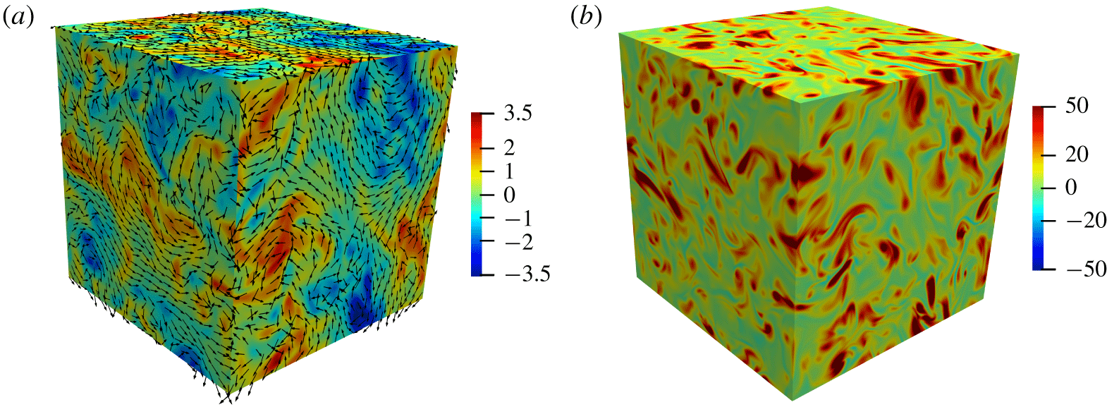
Snapshots of velocity (a) and helicity (b) on the three faces of the cubic resolution domain for  $\unicode[STIX]{x1D700}_{E}=0.2$ and
 $\tilde{\unicode[STIX]{x1D700}}_{H}=25$. In (a) the colours represent the isovalues of the velocity component perpendicular to each face, and the arrows the velocity field parallel to each face. In (b) the colours represent the isovalues of helicity.

In figure 10, snapshots of both velocity and helicity are represented on the three faces of the resolution domain. We see large-scale structures due to the inverse cascade, but the flow is clearly three-dimensional.
Our results are consistent with the dual cascade phenomenology characterized by an inverse cascade of energy with  $E(k)\propto k^{-5/3}$ for
 $k<k_{E}$ and a forward cascade of helicity for
 $k>k_{E}$ (Alexakis & Biferale Reference Alexakis and Biferale2018). Finally our study is also consistent with the experimental results of near-maximum helical turbulence by Herbert et al. (Reference Herbert, Daviaud, Dubrulle, Nazarenko and Naso2012), in which a non-local inverse cascade was identified, but for which an alternative explanation based on axisymmetric turbulence was also invoked (Qu, Naso & Bos Reference Qu, Naso and Bos2018).
Acknowledgements
F.P. and M.K.V. are grateful for support from IFCAM project MA/IFCAM/19/90, and CEFIPRA project 6104-1. M.K.V. and R.S. thank Grenoble Alpes University for support. Our numerical simulations have been performed on Shaheen II at the KAUST supercomputing laboratory, Saudi Arabia, under the project k1416.
Declaration of interests
The authors report no conflict of interest.