1. INTRODUCTION
Terrain Aided Navigation (TAN), which is a good alternative to Global Navigation Satellite Systems (GNSS) in a GNSS-denied environment, has been successfully employed for many applications (Fountain, Reference Fountain1998; Kim et al., Reference Kim, Cho, Lee and Kang2015; Melo and Matos, Reference Melo and Matos2017). When a vehicle passes through a region whose elevation has been surveyed and stored as Digital Elevation Map (DEM) data in advance, the on-board sensors, such as an altimeter and a barometer, acquire real-time elevations for matching with the DEM in a TAN-matching algorithm to estimate an optimal position for the sensor platform. The estimated position can then be used to compensate for an Inertial Navigation System (INS) accumulated position error. Obviously, the matching performance depends significantly on the matching algorithm.
According to the data samples for use in matching, the algorithms can be classified as the single point, the One-Dimensional (1D) sequence, the Two-Dimensional (2D) grey image, and the Three-Dimensional (3D) elevation image (Golden, Reference Golden1980; Hostetler, Reference Hostetler1978; Rodriguez and Aggarwal, Reference Rodriguez and Aggarwal1990; Sjanic and Gustafsson, Reference Sjanic and Gustafsson2015; Venable and Raquet, Reference Venable and Raquet2016; Wu and Ye, Reference Wu and Ye2008; Ye and Chen, Reference Ye and Chen2012). Sandia Inertial Terrain-Aided Navigation (SITAN), a typical single-point algorithm, estimates a vehicle position with just one elevation sample by the Extended Kalman Filters (EKFs) (Hostetler, Reference Hostetler1978). SITAN is useful in real time but poor in its stability. The matching stability can be improved significantly if a sequence of the sampled elevations is employed in a matching process. The typical 1D sequence algorithm is Terrain Contour Matching (TERCOM) (Golden, Reference Golden1980). A sequence of the sampled elevations is matched with the candidate sequences in the reference DEM by the TERCOM matching criteria of Mean Absolute Difference (MAD), Mean Squared Difference (MSD), and/or Cross Correlation (COR). Although TERCOM has been implemented successfully in practice, it is still vulnerable to mismatches due to the terrain similarity in different nearby regions (Meduna et al., Reference Meduna, Rock and McEwen2010). Hence, the samples for one matching should be increased to improve the matching stability further.
If a 2D grey image acquired by an on board camera or a Synthetic Aperture Radar (SAR) or a 3D elevation image acquired by an on board Interferometric SAR (InSAR) is used in a matching process, both the matching accuracy and the matching stability can be significantly improved. The value of a pixel in a 2D grey image is the grey value while it is the elevation in a 3D elevation image, so the reference DEM has to be replaced by the corresponding grey image for matching with a 2D grey image (called ‘scene matching’). Hence, the 2D scene matching can share the matching algorithms with 3D terrain matching. The typical image matching algorithms include correlation, corner or edge detector, and invariant feature (Harris and Stephens, Reference Harris and Stephens1988; Keyes and Winstanley, Reference Keyes and Winstanley2001; Wong and Hall, Reference Wong and Hall1978). The typical correlation algorithm is the aforementioned COR, but it is not invariant to the geometric transformations, such as rotation, translation and scale (Keyes and Winstanley, Reference Keyes and Winstanley2001). The matching algorithm based on a corner or an edge detector, such as a Harris detector or Canny detector (Harris and Stephens, Reference Harris and Stephens1988), is invariant to geometric transformations, but it is sensitive to noise since the detectors are based on difference. Hence, robust invariant features, such as Scale Invariant Feature Transform (SIFT), Speeded-Up Robust Features (SURF), Hu moments, Zernike moments, etc. (Bay et al., Reference Bay, Ess, Tuytelaars and Van Gool2008; Canterakis, Reference Canterakis1999; Hu, Reference Hu1962; Lowe, Reference Lowe2004), have been proposed for matching. The matching algorithms based on invariant features are not only invariant to the geometric transformations but also robust to noise. Particularly, Zernike moments are superior to other invariant features in terms of noise sensitivity, discrimination power and information redundancy since they are orthogonal and expandable to the infinite order (Khotanzad and Hong, Reference Khotanzad and Hong1990; Novotni and Klein, Reference Novotni and Klein2004). Hence, Zernike moments have been employed in a wide range of applications such as pattern recognition, image retrieval, etc. (Clemente et al., Reference Clemente, Pallotta, De Maio, Soraghan and Farina2015; Grandison et al., Reference Grandison, Roberts and Morris2009; Millan et al., Reference Millan, Dempere-Marco, Pozo, Cebral and Frangi2007; Venkatraman et al., Reference Venkatraman, Chakravarthy and Kihara2009). An algorithm based on 3D Zernike Moments (3DZMs) has also been proposed for 3D terrain matching and its feasibility has been tentatively verified (Wu and Ye, Reference Wu and Ye2008; Ye and Chen, Reference Ye and Chen2012). However, 3DZMs' large computation load is a significant barrier for real-time application. Improving the efficiency of computing 3DZMs is always the focus in related fields.
Based on the linear combination of 3D Geometric Moments (3DGMs) for 3DZMs derived by Canterakis (Reference Canterakis1997), the linear combination coefficients are decoupled from their 3DGMs so that the coefficients can be computed independently in advance (Novotni and Klein, Reference Novotni and Klein2004). Therefore, efforts have been mainly devoted to the efficient computation of 3DGMs. On one hand, the fast algorithm for the computation of 2D ordinary geometrical moments has been generalised to 3DGMs (Canterakis, Reference Canterakis1997; Hatamian, Reference Hatamian1986). On the other hand, a symmetry-based method has been proposed to compute 3DGMs with an 87% reduction in the computational complexity (Hosny and Hafez, Reference Hosny and Hafez2012). However, these methods are designed for volumetric images or 3D entities, so they will lose effectiveness for 3D elevation images in terrain matching. Obviously, the complexity of the volume integral O(N3) is higher than the surface integral O(N2). The surface-like geometric moments, instead of the volume-like geometric moments, have also been proposed to compute 3DZMs. Unfortunately, they are designed for unstructured 3D entities by triangle meshes (Pozo et al., Reference Pozo, Villa-Uriol and Frangi2011) so they are unsuitable for the elevation surface in structured templates using square meshes.
3D Pseudo Zernike Moments (3DPZMs) are similar to 3DZMs except that 3DPZMs are based on pseudo-Zernike instead of Zernike radial polynomials. It is reported that 3DPZMs are better in noise tolerance than 3DZMs to some extent (Al-Rawi, Reference Al-Rawi2012). However, 3DPZMs are nonlinear to their 3DGMs so that all parts of 3DPZMs have to be computed online. Even though the symmetry properties of spherical harmonics and recursive radial polynomials have been used to speed up the 3DPZMs' computation (Al-Rawi, Reference Al-Rawi2012), the online computation load is still unacceptable for real-time applications. Hence, 3DPZMs will not be studied here.
In this paper, a real-time terrain matching algorithm based on 3DZMs is proposed for land applications. In the new algorithm development presented, two new efficient methods based on coordinate transformation and symmetry properties are proposed to compute 3DGMs without approximation. In addition, the terrain feature vectors based on the 3DZMs are computed offline in advance and stored for the reference DEMs after the feasibility of using a circular template is proven. Only the terrain feature vectors of Real-time Elevation Maps (REMs) are computed online so that the online computation load will be significantly reduced.
The remainder of the paper is organised as follows: The definition of 3DZMs and the terrain matching algorithm based on 3DZMs will be described in Section 2. To improve the real time performance of the new matching algorithm, two efficient methods based on coordinate transformation and symmetry properties are proposed to reduce the online computation load in Section 3. In Section 4, the impact of the sample difference between DEMs and REMs will be investigated to confirm the feasibility of the circular template. The proposed algorithm is verified by numerical experiments in Section 5 and concluding remarks are provided in Section 6.
2. TERRAIN MATCHING ALGORITHM BASED ON 3DZMS
This section briefly presents the definition of 3DZMs and descriptors, and details can be found in the literature (Khotanzad and Hong, Reference Khotanzad and Hong1990; Novotni and Klein, Reference Novotni and Klein2004). The terrain matching algorithm based on 3DZMs will be described. Both DEM and REM are stored in the form of a square grid. The terrain feature vectors of a reference map are computed offline and stored for subsequent matching. The terrain feature vector of a REM is computed online to match with those of the reference map using a criterion.
2.1. 3DZMs and descriptors
The 3DZMs used for feature extraction in terrain matching can be defined as:
 $$\Omega _{nl}^m = \displaystyle{3 \over {4\pi }}\sum\limits_{r + s + t \le n} {\overline {\chi _{nlm}^{rst} } } M_{rst}$$
where  $\Omega_{nl}^{m}$ is a 3D Zernike moment; n, l and m are integers, n ∈ [0, Max], l∈[0, n], m∈[−l, l], Max is the maximum order of the moment, and (n−l) must be an even number; the combinatorial coefficients
 $\chi_{nlm}^{rst}$ are determined by the six integers n, l, m, r, s and t,
 $\overline{\chi_{nlm}^{rst}}$ is the complex conjugate of
 $\chi_{nlm}^{rst}$ and M rst is the geometric moment. The values of
 $\chi_{nlm}^{rst}$ for r + s + t ≤ n can be computed independently offline. The geometric moment M rst is defined as:
 $$M_{rst} = \int_{\vert x\vert \le 1} f \lpar {\bf x}\rpar x^ry^sz^t\hbox{d}{\bf x}$$
where x = (x, y, z) T, f(x) = 1 if the points locate on the terrain surface, otherwise f(x) = 0. Hence, the discrete form of M rst under the assumption of a unit cube pixel is:
 $$M_{rst} = \sum\limits_{i = 1}^N {x_i^r } y_i^s z_i^t$$
where x i, y i and z i are the i-th sample in the normalised coordinate and N is the number of samples.
It should be noted that the 3D Zernike moments  $\Omega_{nl}^{m}$ are not invariant under rotation, but the 3D Zernike descriptor F nl is rotationally invariant. F nl is defined as:
 $$F_{nl} = \left\Vert {{\left[ {\Omega_{nl}^l \comma \; \Omega_{nl}^{l - 1} \comma \; \Omega_{nl}^{1 - 2} \comma \; \cdots \comma \; \Omega_{nl}^{ - l} } \right] }^T} \right \Vert $$
where ‖a‖ is the norm of the vector a.
2.2. Matching criterion
3D elevation images can be equivalently represented by 3DZMs from zero order to infinite order (Canterakis, Reference Canterakis1999). Hence, the feature vector Fn based on 3D Zernike descriptors can be formed as:
 $${\bf F}^n = \left[{\matrix{ {F_{20}} & {F_{22}} & {F_{31}} & \cdots & {F_{nn}} \cr } } \right]^{\rm T}$$
F 00 and F 11 are not included in Equation (5), which will be explained in Section 3. With the maximum order n increasing, the feature vector can present the terrain fluctuation more accurately, but the computation of the feature vector will also increase significantly. Hence, n should be as small as possible to reduce the computation load if the terrain feature has been sufficiently extracted. It has been verified that the maximum order ten can achieve high enough accuracy in the terrain feature extraction for matching (Ye and Chen, Reference Ye and Chen2012).
In the terrain matching with a 1D elevation sequence, MSD, MAD and COR have been widely used to evaluate the similarity between the real-time sequence and the references. However, the values of the 3D Zernike descriptors vary significantly with their orders. For example, F 20 may be far greater than F 22. It is also unreasonable to allocate the same weight to 3D Zernike descriptors with different dimensions. Hence, the Canberra distance (Ye and Chen, Reference Ye and Chen2012) is employed as the matching criterion to evaluate the similarity between two feature vectors to balance the contribution of the elements in them. The Canberra distance is defined as:
 $$d\lpar {\bf p}\comma \; {\bf q}\rpar = \sum\limits_{j = 1}^K {\left\vert {\displaystyle{{p_j - q_j} \over {p_j + q_j}}} \right\vert }$$
where p and q are two K-dimensional vectors and p j + q j ≠ 0. According to Equation (6), the lower the value of the Canberra distance, the more similar the two vectors are, and vice versa.
2.3. Terrain matching algorithm
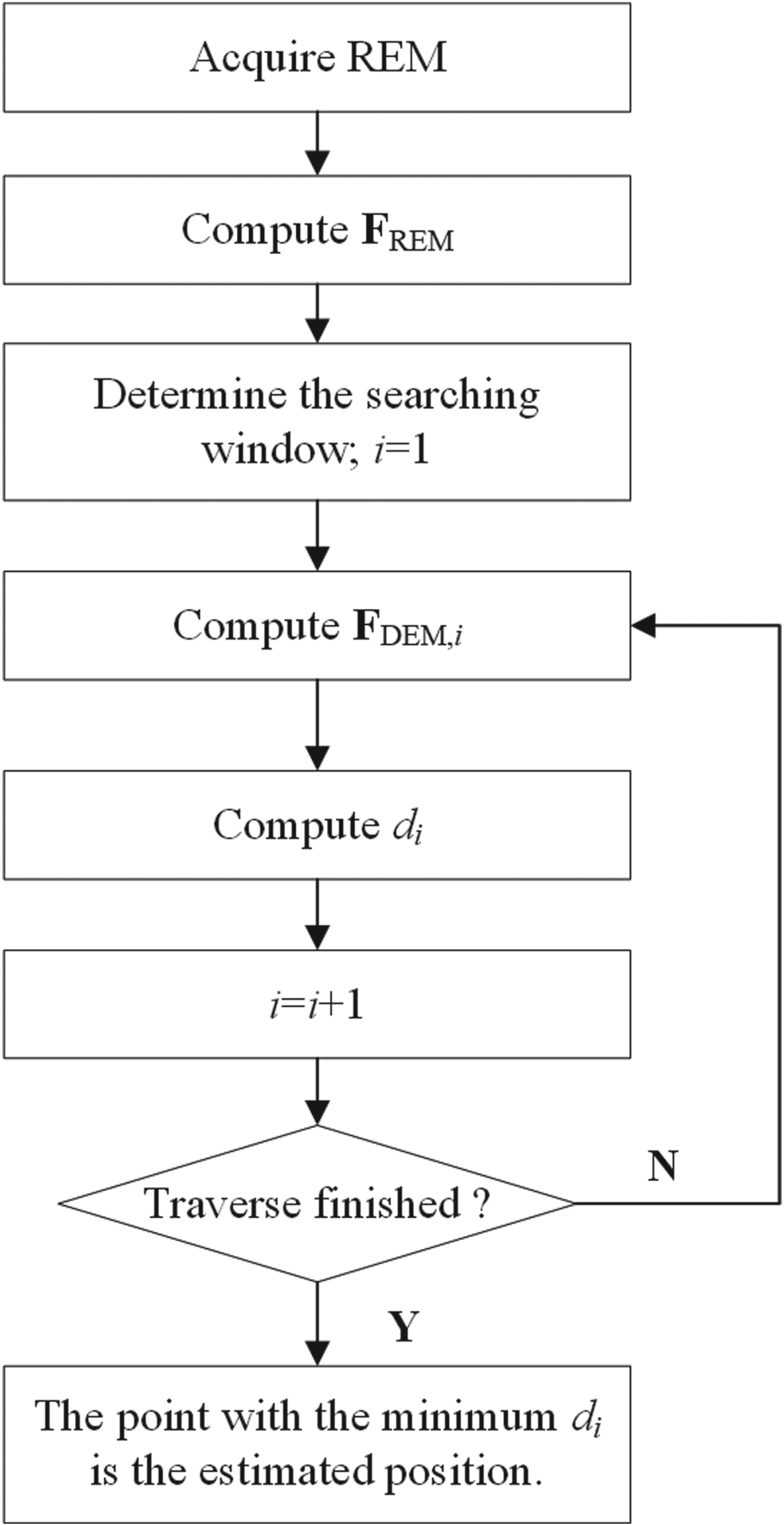
It is assumed that the REM grid resolution is the same as the DEM. The maximum order of 3DZMs and the size of the matching template are determined in advance. For simplification, the REM is the same size as the matching template. Hence, for a given REM, the procedure of the proposed real-time terrain matching algorithm based on 3DZMs illustrated in Figure 1 is described as follows:
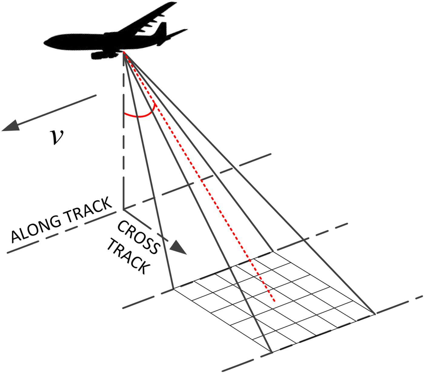
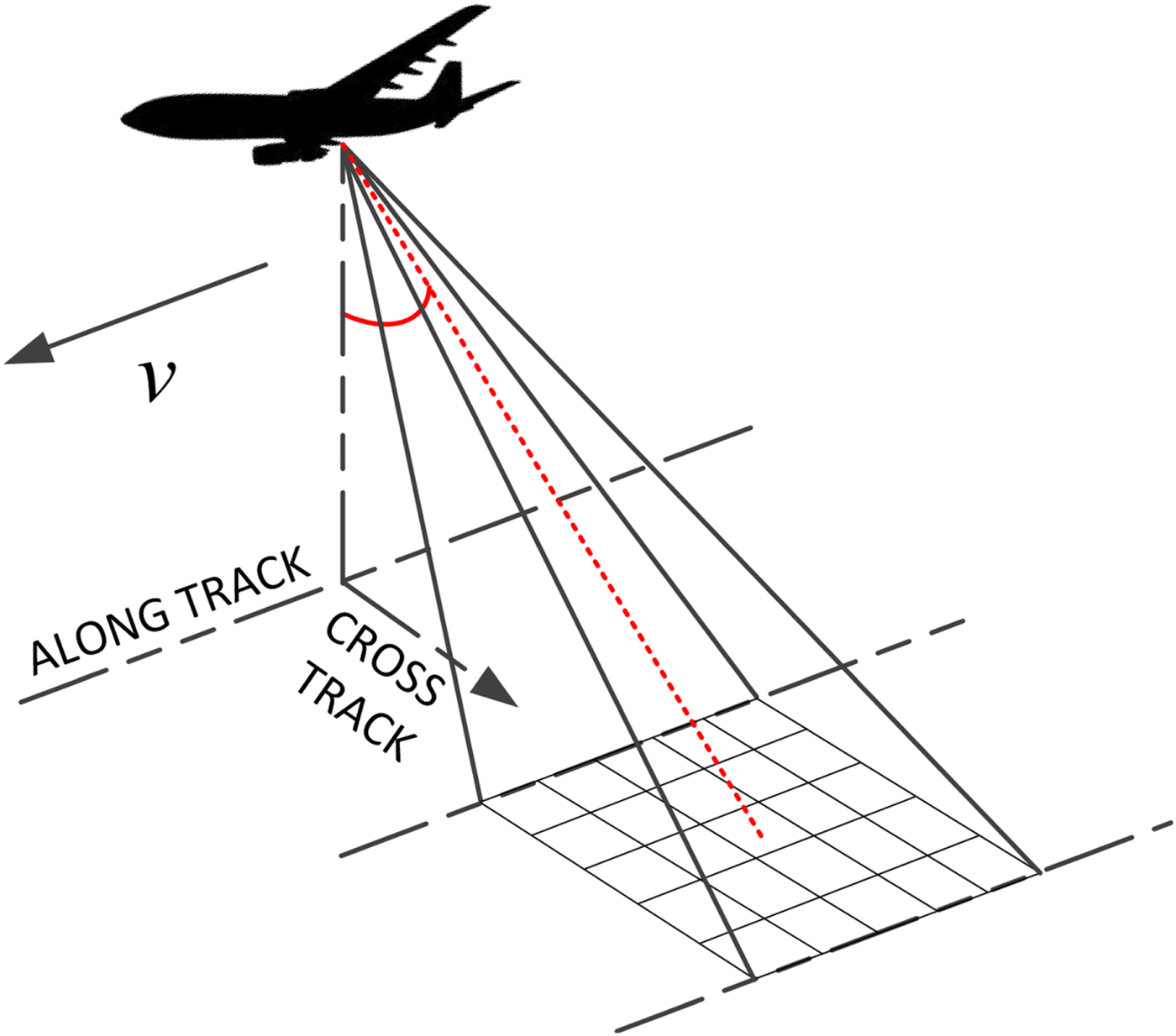
(1) Sample the REM data as depicted in Figure 2 and compute the feature vector FREM of the REM by Equations (1)–(5).
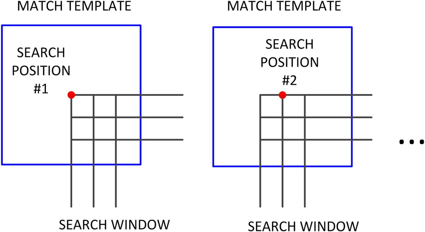
(2) Determine the searching window in a reference DEM. The size of the searching window is determined by the estimated error of the current position, usually provided by an INS.
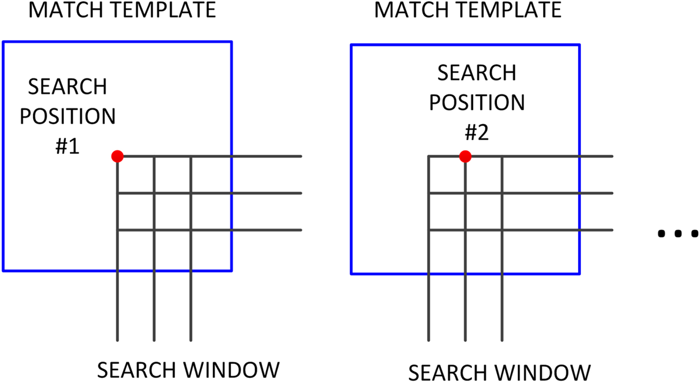
(3) Slide the matching template on the grid points in the searching window. Compute the feature vector FDEM,i of the reference DEM in the template at the i-th grid point.
(4) Compute the Canberra distance between the feature vectors FREM and FDEM,i by Equation (6).
(5) Traverse the searching window point by point as shown in Figure 3.
(6) The point with the minimum d i is determined as the optimal estimation of the true position.
Flowchart of the proposed terrain matching algorithm.

Acquisition of REM.
Traverse in the searching window.
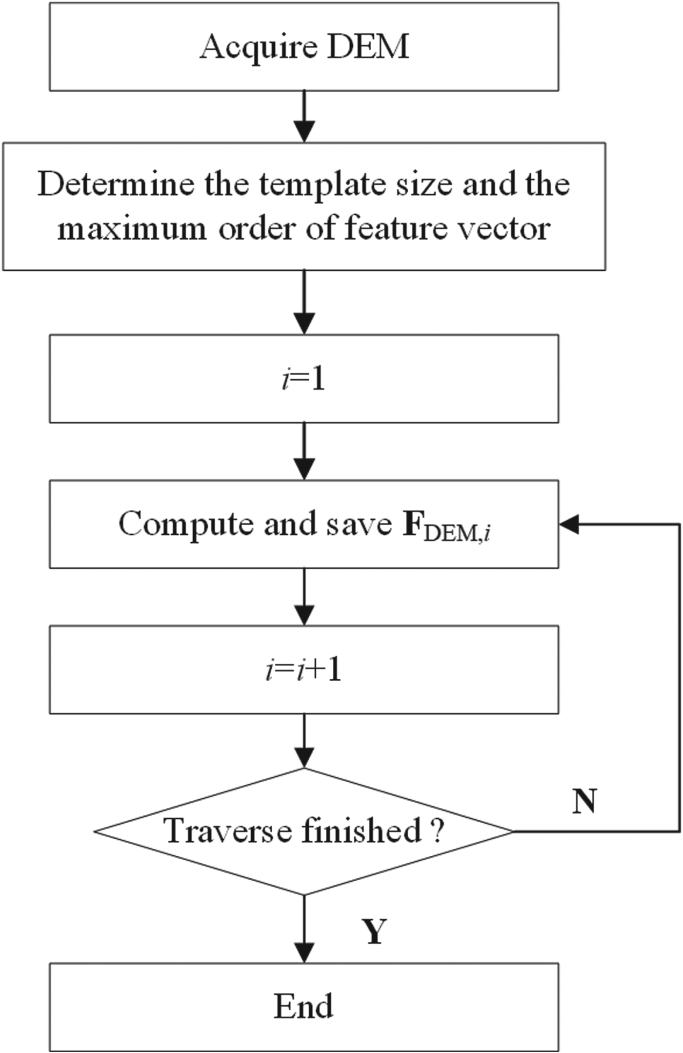
Two innovative approaches which can achieve matching results in real time are proposed here. One approach is the efficient method to compute the geometric moments which will be detailed in Section 3. The other is the offline computation of the feature vectors of the reference DEM based on a circular template. The feasibility of the circular template will be proven in Section 4. The flowchart of computing the feature vectors of the reference DEM off-line is illustrated in Figure 4.
Flowchart of the offline computation of the feature vectors of the reference DEM.

3. EFFICIENT METHODS TO COMPUTE THE GEOMETRIC MOMENTS
Since the combinatorial coefficients have been computed offline in advance, the geometric moments consume most of the online time in computing 3DZMs. Here, an efficient method is proposed to separate the items unrelated to the elevation from the 3DGMs' computation by the coordinate transformation. The symmetry of the integral domain is also taken into account to further reduce the computation load.
3.1. Coordinate transformation and separation
In a terrain matching process, the REM size is determined in advance and fixed. The Candidate Elevation Maps (CEMs) in the reference DEM have the same size as the REM. Hence, the 3DZMs of the REM and the CEMs are only the functions of elevation, which provides the opportunity to compute the items related to x and y independently.
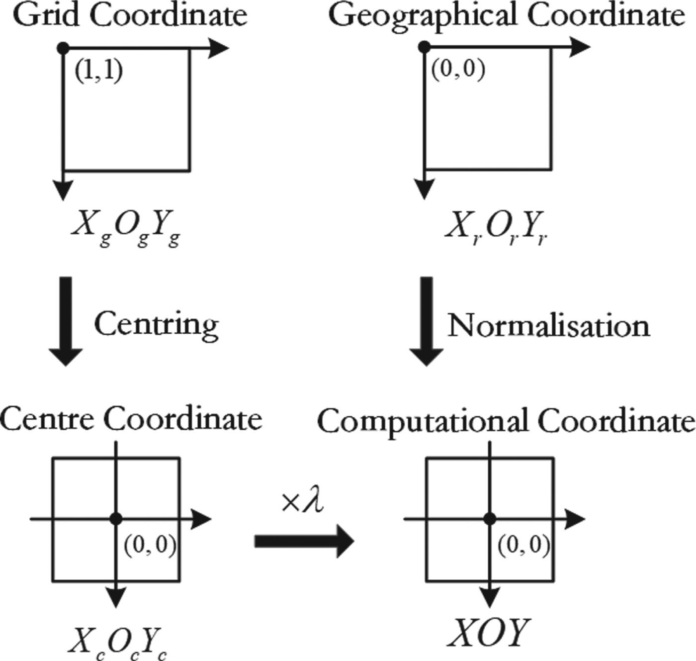
Figure 5 depicts the relationship among the different coordinates. The start point of the grid coordinates is (1,1) and the map size in the grid coordinate is measured by its grid number. What is different in the geographical coordinate or measurement coordinate is that the start point is (0,0) and the unit of the map size is a metre. The grid distance in the geographical coordinate equals the resolution of the reference DEM. It is necessary to move the origin of the map in the geographical coordinate to its centre and normalise its three coordinate values before the 3DGMs computation. Equivalently, the reference DEM, stored in grid coordinates, can be transformed to the computational coordinate by centring and normalising by a scale λ.
Sketch of the coordinate transformation.

After the normalisation, xr, ys, and zt can be computed. This avoids redundant computation when they are reused in 3DGMs. Furthermore, according to the relationship in Figure 5, Equation (3) can be rewritten as:
 $$M_{rst} = \sum\limits_{i = 1}^N {{\lpar \lambda x_{ci}\rpar }^r} \lpar \lambda y_{ci}\rpar ^sz_i^t = \lambda ^{r + s}\sum\limits_{i = 1}^N {\lpar x_{ci}^r y_{ci}^s \rpar } z_i^t$$
where the scale λ has the following relationship:
 $$\lambda = \displaystyle{{x_i} \over {x_{ci}}} = \displaystyle{{y_i} \over {y_{ci}}}$$
In Equation (7), x ci and y ci are the centralised coordinates in the centre coordinate and unrelated to the grid distance and the elevation z i. Hence, the item  $x_{ci}^{r} y_{ci}^{s}$ can be pre-computed offline and stored so that the exponentiations of
 $x_{ci}^{r}$ and
 $y_{ci}^{s}$ and the multiplication of
 $x_{ci}^{r} y_{ci}^{s}$ are saved in the online computation. In computing M rst, there are N × (r + s + t − 4) multiplications in Equation (3), but only N × (t − 1) multiplications are required in Equation (7).
Furthermore, the reuse of 3DGMs is also employed here to significantly reduce the online computation since 3DGMs have been reused frequently in 3DZMs computation.
3.2. Symmetry properties
The coordinates of x, y and z after normalisation are symmetrical. That is:
 $$\sum\limits_i^N {x_i} = 0\comma \; \quad \sum\limits_i^N {y_i} = 0\comma \; \quad \sum\limits_i^N {z_i} = 0$$
In addition, if t = 0, there is:
 $$M_{rs0} = \sum\limits_{i = 1}^N {x_i^r } y_i^s = \sum\limits_{i = 1}^N {x_i^s } y_i^r = M_{sr0}$$
Moreover, if t = 0 and r or s is odd, there is:
 $$M_{rs0} = \sum\limits_{i = 1}^N {x_i^r } y_i^s = 0$$
Hence, Equation (7) can be specified as:
 $$M_{rst} = \left\{{\matrix{ 0 \hfill & {t = 0\semicolon \; \; r = \hbox{odd or}\; s = \hbox{odd}} \hfill \cr {\lambda^{r + s}\sum\limits_{i = 1}^N {x_{ci}^r } y_{ci}^s } \hfill & {t = 0\semicolon \; \; r = \hbox{even}\semicolon \; \; s = \hbox{even}} \hfill \cr {\sum\limits_{i = 1}^N {z^t} } \hfill & {t \ne \; 0\semicolon \; r = 0\semicolon \; s = 0} \hfill \cr {\lambda^{r + s}\sum\limits_{i = 1}^N {x_{ci}^r } \; y_{ci}^s z^t} \hfill & {\hbox{others}} \hfill \cr } } \right.$$
According to Equation (1), there is:
 $$\Omega _{11}^0 = \displaystyle{3 \over {4\pi }}\overline {\chi _{110}^{001} } M_{001} = \displaystyle{3 \over {4\pi }}\overline {\chi _{110}^{001} } \sum\limits_{i = 1}^N {z_i} = 0$$
 $$\Omega _{11}^1 = \displaystyle{3 \over {4\pi }}\lpar {\overline {\chi_{111}^{010} } M_{010} + \overline {\chi_{111}^{100} } M_{100}} \rpar = \displaystyle{3 \over {4\pi }}\left({\overline {\chi_{111}^{010} } \sum\limits_{i = 1}^N {y_i} + \overline {\chi_{111}^{100} } \sum\limits_{i = 1}^N {x_i} } \right)= 0$$
Substituting Equations (13) and (14) into Equation (4) yields:
 $$F_{11} = \left\vert {{\left[ {\Omega _{11}^1 {\rm ,}\,\;\Omega _{11}^0 {\rm , }\;\Omega _{11}^{ - 1} } \right]}^{\rm T}} \right\vert = 0$$
Moreover, there is:
 $$F_{00} = \Vert {\Omega_{00}^0 } \Vert = \Vert {M_{000}} \Vert = \left\Vert {\sum\limits_{i = 1}^N {x_i^0 } y_i^0 z_i^0 } \right\Vert = N$$
According to Equations (15) and (16), the first two descriptors F 00 and F 11 are independent of elevation, so they are excluded from the feature vector in Equation (5).
4. CIRCULAR TEMPLATE
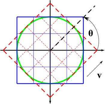
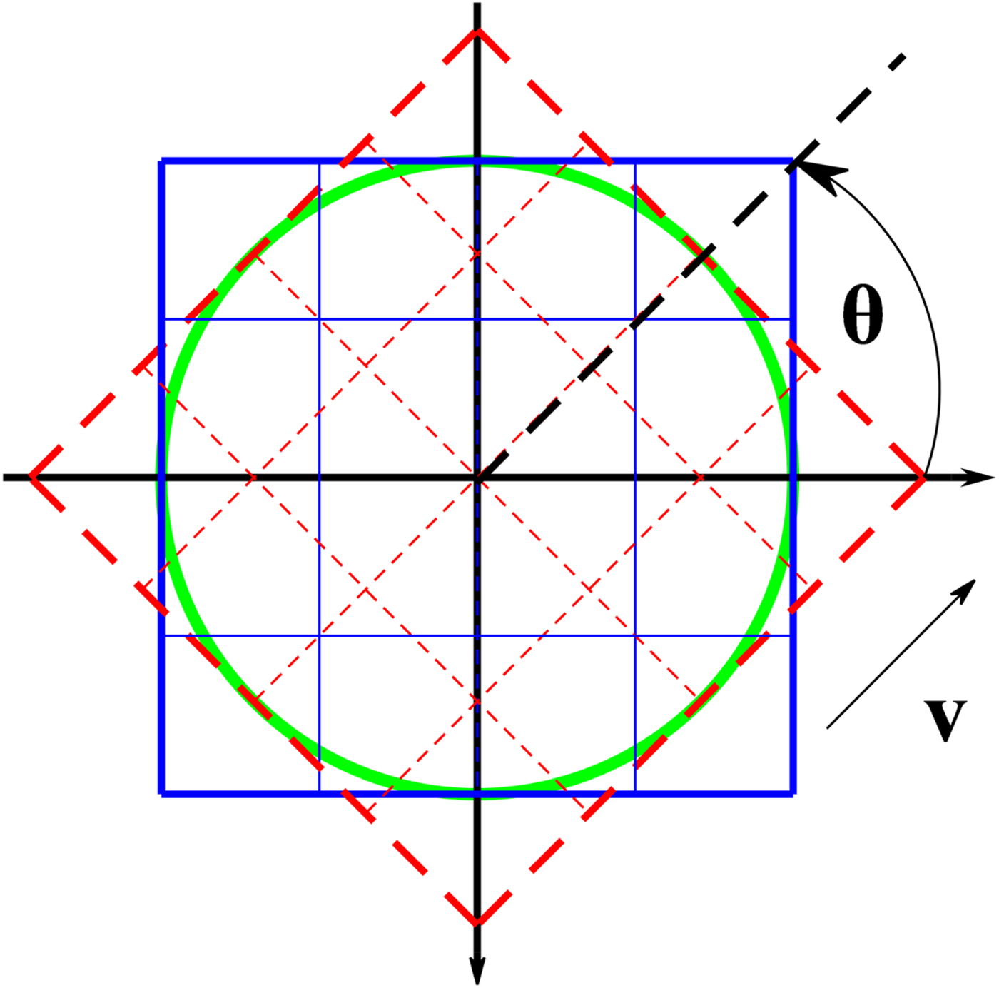
When a vehicle passes through a region there is usually an angle between the acquired REM and the stored DEM, which is called a heading angle hereinafter. As mentioned above, the 3D Zernike descriptors are rotationally invariant, but the condition is that the samples in the REM and the DEM should be the same. Otherwise, the difference between the 3D Zernike descriptors of the REM and those of the DEM may be very large due to the sample difference. As illustrated in Figure 6, the heading angle between the REM shown in the dashed square and the DEM shown in the solid square is θ. The velocity v shows the moving direction of the vehicle. In Figure 6, not only are the samples in the un-overlapped areas of the two maps different but also those in the overlapped areas are different, which leads to computation errors in 3D Zernike descriptors. The Canberra distance caused by the sample difference is contributed by the following three parts,
 $$\hat d\lpar \Delta x\comma \; \Delta y\comma \; \theta \rpar \colon \lcub d\lpar \Delta x\comma \; \Delta y\rpar \comma \; \Delta d_{\rm u}\lpar \Delta x\comma \; \Delta y\comma \; \theta \rpar \comma \; \Delta d_{\rm o}\lpar \Delta x\comma \; \Delta y\comma \; \theta \rpar \rcub$$
where d̂ is the real Canberra distance which is the function of the position difference (Δx, Δy) and the heading angle θ, d is the Canberra distance without rotation and Δd u and Δd o are the Canberra distance errors due to the un-overlapped and the overlapped areas, respectively. Obviously, Δx = Δy = 0 in Figure 6 so that d = 0, but d̂ does not definitely equal 0 due to the existence of Δd u and Δd o when θ = 0. Hence, the heading angle will influence the matching.
Sample difference between REM and DEM.
One method to solve the problem is to rotate the DEM according to the current heading angle measured by the INS, but the rotation is very time-consuming, and it could be even worse when the rotation is biased by the heading angle error. It is less time-consuming to rotate the REM, but the impact of the heading angle error and interpolation error still exists.
The other method is to use a circular template to replace the square one in matching which has been employed in a 2D image processing (Choi and Kim, Reference Choi and Kim2002; Revaud et al., Reference Revaud, Lavoue and Baskurt2009). There is still the sample difference between the REM and the DEM as the circle illustrated in Figure 6, but the REM will totally overlap the DEM with a circular template if there is no position difference between the REM and the DEM. That is, Δd u will disappear if a circular template is employed, but the impact of Δd o still exists.
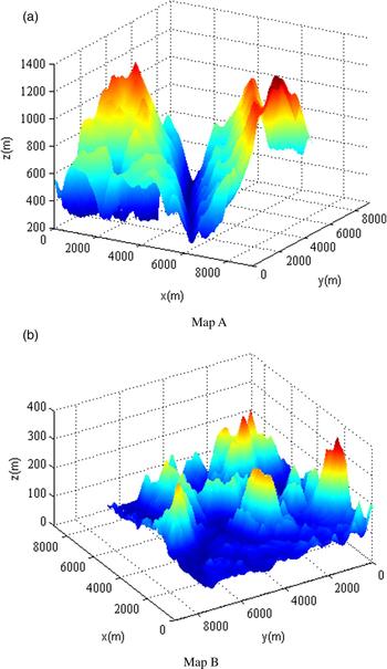
To illustrate the impact of the heading angle on the feature vector with the two templates, two reference DEMs obtained from the Advanced Spaceborne Thermal Emission and Reflection Radiometer Global Digital Elevation Model (ASTER GDEM) (Tachikawa et al., Reference Tachikawa, Hato, Kaku and Iwasaki2011) shown in Figure 7 are taken as an example. The standard deviations of the two maps are 235·72 m and 45·34 m respectively, and the grid resolution is 30 m. Obviously, Map A fluctuates more significantly than Map B.
3D images of the two reference maps.
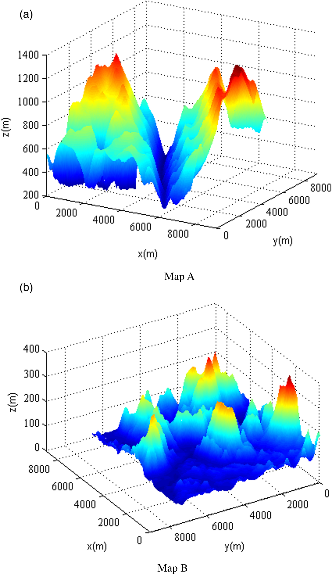
For the square template, the sizes of the maps and the REMs are 300 × 300 grid and 80 × 80 grid respectively, but the REMs are the inscribed circles of a square for the circular template. In order to evaluate the impact of the heading angle independently, the REMs are extracted directly from the reference DEM and no noise is added. In addition, when the samples of the rotated REMs do not locate on the grid points, their elevations are determined by bilinear interpolation.
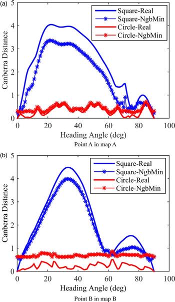
Figure 8 depicts the Canberra distances with the heading angle at two points in Maps A and B, which represent the typical results in the maps. Due to the rotational invariance, the Canberra distances change periodically with the heading angle and the period is 90°. Consequently, the range of the heading angle in Figure 8 is from 0° to 90°. Feature vectors in REMs under different heading angles and CEMs without rotation are computed. Canberra distances between REMs and CEMs using the square template (labelled ‘Square’ in Figure 8) are compared with those using the circular template (labelled as ‘Circle’ in Figure 8). Since the mismatching is most likely to happen in the vicinity of the real position, Canberra distances at the real positions (labelled ‘Real’ in Figure 8) are compared with the minimum Canberra distances among the 24-neighbour grids, that is, the 5 × 5 grid window without the centre of the real positions (labelled ‘NbgMin’ in Figure 8).
Canberra distances with the heading angle without the position error.
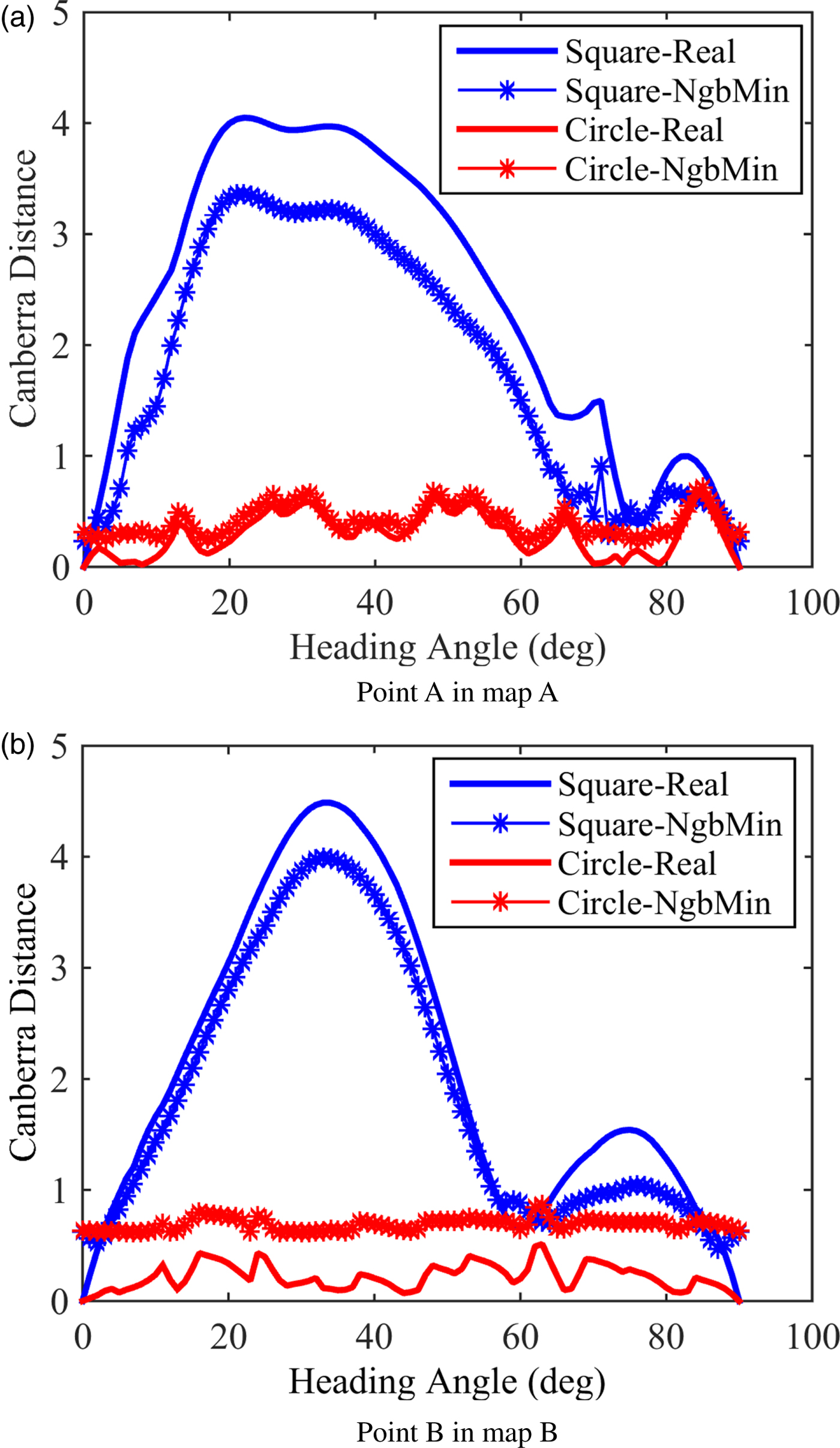
The matching is correct if the Canberra distance at the real position is the minimum. In Figure 8, the Canberra distances at the real positions are always less than the minimum Canberra distances among the 24-neighbour grids in the two maps if the circular template is used. This means that the impact of the heading angle on the matching can be ignored if the circular template is employed. In contrast, when the square template is employed, the Canberra distances at the real positions are always greater than the minimum Canberra distances among the 24-neighbour grids in the two maps unless the heading angle is close to 0° or 90°. Hence, the impact of the heading angle on the matching is significant if the square template is used. The main reason is that the contribution of the un-overlapped areas in the square template is significant while the sample difference in the circular template is tolerable to some extent.
The elevation measurement error is not taken into account in Figure 8, so the impact of the heading angle on the matching algorithm with the elevation measurement error will be evaluated further by numerical experiments in the next section.
If matching with the circular template is feasible, the terrain feature vectors of the reference map can be computed offline to significantly reduce the online computation, which provides the basis for the real-time matching algorithm proposed in Section 2.
5. NUMERICAL EXPERIMENTS
In this section, the feasibility of matching with a circular template and the superiority of the proposed terrain matching algorithm based on 3DZMs is verified by numerical experiments. The proposed efficient methods to compute 3DZMs and the real-time matching algorithm is also validated.
In the experiments, the maximum order of 3DZMs is ten. The searching window is a 100 × 100 grid square area and the size of the square template is a 80 × 80 grid. The circular template is the inscribed circle of the square template. The REMs are acquired by adding a Gaussian white noise to the reference DEM. As addressed in Section 4, if the samples of the REMs do not locate at the grid points, their elevations are determined by bilinear interpolation. That is, the samples of the REMs are usually not the same as those of the reference DEM.
All of the algorithms were programmed in MATLAB and ran on a computer with an Intel Core i5-3470 CPU (Central Processing Unit) (3·2GHz) and 4GB of random access memory.
5.1. Circular template
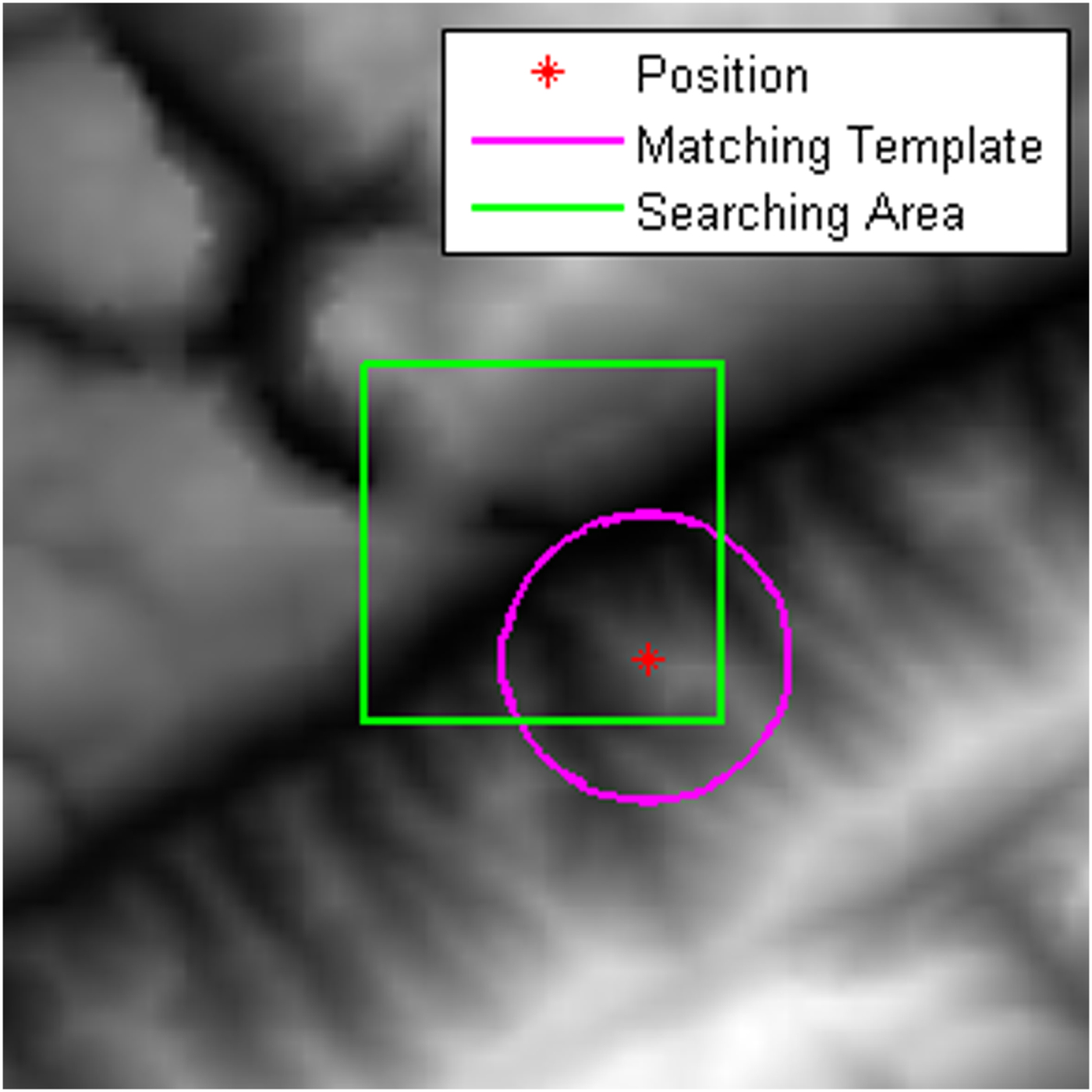
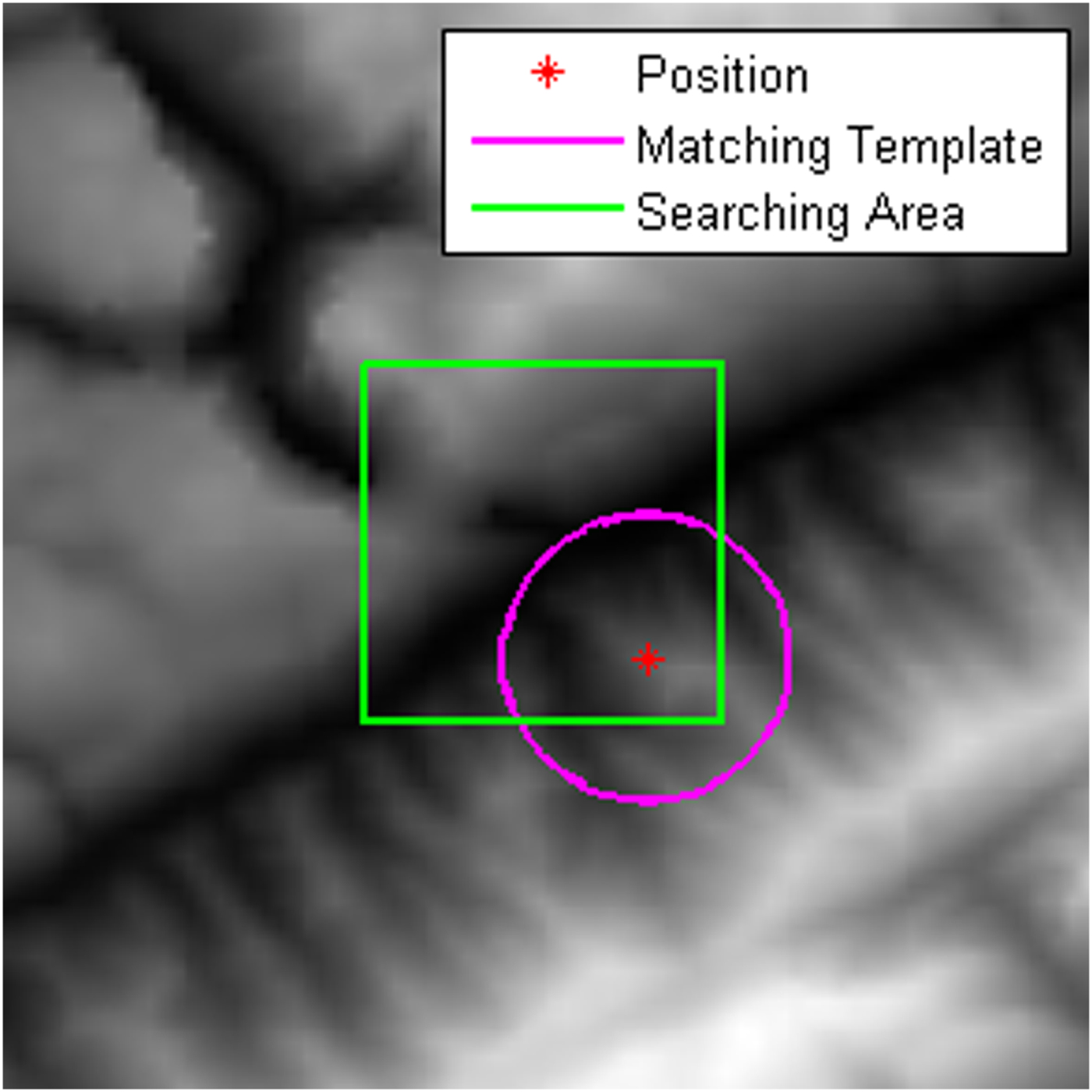
The numerical experiments are performed in the two maps shown in Figure 7. Figure 9 depicts the searching area and a CEM. 1,000 REMs were randomly acquired to derive the matching statistics herein. Since the REM centre does usually not locate on a grid point, the matching is correct if the matching error is less than  $\sqrt{2}$ times a grid distance.
Searching window and a CEM.
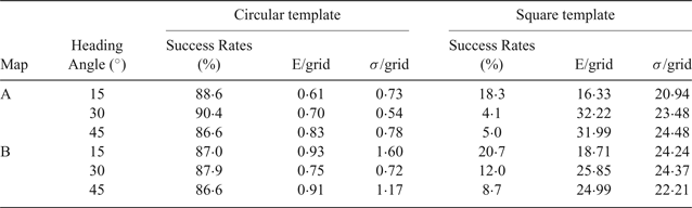
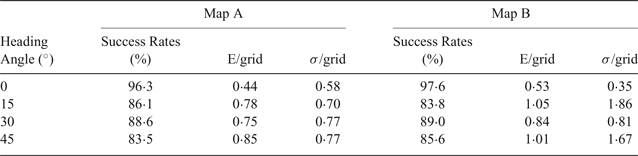
The statistics of the matching results with and without noise are listed in Tables 1 and 2 respectively. To investigate the anti-noise capability of the matching algorithm, the REMs had zero-mean Gaussian white noise added with a standard deviation of 5 m, as shown in Table 2. Since the matching algorithm with the square template failed to find the correct positions with a high success rate under the noise-free condition in Table 1, only the matching results with the circular template are presented in Table 2.
Matching errors without noise.

Matching errors with noise.
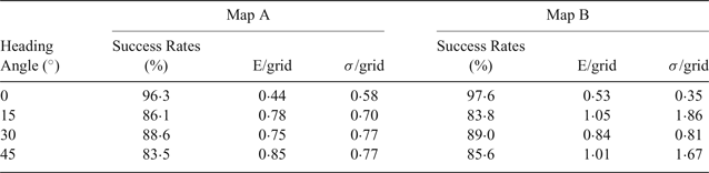
As listed in Table 1, the success rate of matching with the square template under rotation is lower than 25% in the two maps. Meanwhile, the matching errors are far greater than one grid. Hence, the heading angle significantly influences the matching with the square template, which coincides with the analysis in Section 4.
In contrast, the success rate of matching with the circular template is very high in the two maps, even though the heading angle is as large as 45°. In fact, the matching results with the circular template are very stable in the two maps as listed in Table 1 when the heading angle is changing. The mean and the standard deviations of the matching errors in Map A are a little greater than those in Map B with the same heading angles, but the difference between them is not significant. When the noise is added into the REMs, the matching results with the circular template in Table 2 are almost the same as those without noise in Table 1. It can also be seen in Table 2 that the success rate of matching are greater than 96% in the two maps when the heading angle is zero. However, it is very difficult to reduce the heading angle to zero in applications. In fact, the success rate of matching in the two maps is not less than 83%, as listed in the two tables, even when there is noise and the heading angle is as large as 45°. Hence, matching with the circular template is robust to the heading angle, the maps with the different fluctuations and noise, which provides a solid foundation for the circular template to be employed in terrain matching.
5.2. Efficient methods to compute 3DZMs
The following three methods are compared by experiments. Method A was proposed by Novotni and Klein (Reference Novotni and Klein2004), which has been widely used. Methods B and C are proposed in this paper.
(1) Method A: The combinatorial coefficients are computed offline and stored for online look-up. The geometric moments are reused in its online calculation for a map.
(2) Method B: Except for the methods used in Method A,
 $x_{i}^{r}$, $y_{i}^{s}$, and $z_{i}^{t}$ are computed separately online for a map to avoid redundantly computing them in calculating $x_{i}^{r} y_{i}^{s} z_{i}^{t}$.
(3) Method C: Except for the methods used in Method A,
$x_{ci}^{r} y_{ci}^{s}$ is computed offline and $z_{i}^{t}$ is computed separately online for a map. The symmetry of the geometric moments shown in Equation (12) is also implemented.


In the above three methods, F 00 and F 11 are not included in the feature vector. Here, only the results with the circular template are presented.
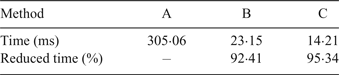
Table 3 identifies the time consumed by each of the three methods to compute the feature vector once. The reduced times for Methods B and C are presented in percentages by comparing with the time consumed by Method A. According to Table 3, it is very effective to reduce the computation load by calculating  $x_{i}^{r}$,
 $y_{i}^{s}$, and
 $z_{i}^{t}$ separately. The time for Method B compared with Method A can be reduced by more than 92%. Moreover, compared with Method B, more than 38% time can be saved by taking advantage of the symmetry of the geometric moments by using Method C. Hence, it is desirable to employ Method C to compute the feature vector.
Time to compute the terrain feature vector once.
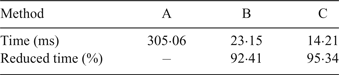
Time consumed for matching algorithm.

5.3. Real-time terrain matching
If the circular template is employed, the feature vectors composed of the 3D Zernike descriptors can be computed offline in advance for the reference DEM, which makes real-time matching possible. Since Method C is the fastest among the three methods to compute the feature vector, it is employed here to evaluate the real-time performance in terrain matching.
The matching to acquire the results in Table 3 is considered again. The searching window is a 100 × 100 grid square. If no searching algorithm is employed, that is, all of the candidate grid points in the searching window are traversed one by one, 10,000 feature vectors are computed in the reference map, which consumes 143·22 s. The extra time is used to compute the feature vector for the REM, the Canberra distances, and so on. Hence, it is impossible to implement the matching algorithm in real time.
The Coarse-To-Fine (CTF) searching algorithm (Ye and Chen, Reference Ye and Chen2012) can be employed to speed up terrain matching. In our implementation, the moving step is ten grids in the coarse matching and the best three candidate points are selected for fine matching. At each candidate point, the matching is performed in a 20 × 20 grid searching window and the moving step is one grid. The point with the minimum Canberra distance in the three searching areas is determined as the final estimation of the real position. The maximum order of 3DZMs is ten for both the coarse and fine matchings. The consumed time is 17·28 s for the matching, so it is still too slow for real-time applications. Meanwhile, the CTF searching increases risk for mismatching due to the searching interval.
To further speed up the matching, the feature vectors of the reference DEM are computed offline in advance. Since the circular template is employed, the offline calculation of the feature vectors is feasible. In the matching, all the grid points in the searching window are traversed one by one. The consumed time is only 0·127 s for matching and thus real-time matching performance can be achieved.
It should be noted that real-time matching is achieved by computing and storing the feature vectors of the reference DEM in advance. If the DEM is as large as M × N grid in size and the maximum order of 3DZMs is ten, the storage for the feature vectors will be M × N × 34 in size. This means that the storage for the feature vectors will be 34 times that for the DEM, which is less than those for SIFT (128 times) or SURF (64 times). Hence, the storage need is moderate.
5.4. Comparison with another terrain matching algorithm
In order to verify the superiority of the proposed terrain matching algorithm based on 3DZMs, a terrain matching algorithm (Song et al., Reference Song, Bian and Adam2016) is compared under the same conditions. The feature vector of the algorithm is composed of ten terrain features. That is:
 $${\bf F} = \left[{\matrix{ {\alpha_1E} & {\alpha_2I} & {\alpha_3C} & {\alpha_4L} & {\alpha_5\bar z} & {\alpha_6\sigma^{\prime}} & {\alpha_7r} & {\alpha_8R} & {\alpha_9H_{\rm f}} & {\alpha_{10}H_{\rm e}} \cr } } \right]^{\rm T}$$
where E, I, C and L are energy, contrast, correlation and inverse difference moment extracted from the grey level co-occurrence matrix of an image respectively;  $\bar{z}$, σ′, r, R, H f and H e are mean of elevation, standard deviation of elevation, terrain roughness, correlation coefficient, entropy, and difference entropy of a region, respectively, and α i(i = 1, 2, · · · , 10) is the weight which has the same value as that in the literature (Song et al., Reference Song, Bian and Adam2016). The definitions of the features can be found in Baraldi and Parmiggiani (Reference Baraldi and Parmiggiani1995) and Ma and Zhao (Reference Ma and Zhao2012).
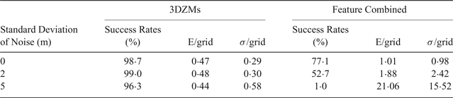
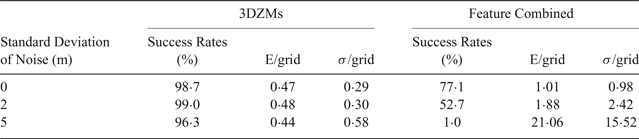
Table 5 lists the matching errors of the proposed 3DZMs algorithm and the feature-combined algorithm (Song et al., Reference Song, Bian and Adam2016) in Map A. Since the latter fails to match if the heading angle is as large as 15°, 30° or 45°, only the results without rotation are provided in Table 5. Obviously, the feature-combined algorithm fails to work when the standard deviation of noise is as large as 5 m since its success rate of matching is as low as 1% while the matching error is very high. In fact, the success rate of the feature-combined algorithm is no more than 80% even though there is no noise. Contrarily, the success rate of the proposed 3DZMs algorithm is more than 96% even though the standard deviation of noise is as large as 5 m. Hence, the proposed 3DZMs algorithm is better than the feature-combined algorithm in robustness both to rotation and to noise. The main reason that the feature-combined algorithm achieves a good performance in Song et al. (Reference Song, Bian and Adam2016) and may be due to ignoring the sample difference between REM and DEM since the grid resolution is as high as 1 m. However, the grid resolution here is as low as 30 m so that the sample difference has to be taken into account.
Matching errors with noise in Map A.
6. CONCLUSION
A real-time terrain matching algorithm based on 3DZMs has been developed to take advantage of the good performance of the 3D Zernike descriptors, which are implemented in a novel and efficient way here to achieve real-time performance for the first time. Three key conclusions are:
(1) An efficient method based on coordinate transformation and symmetry properties has been proposed to speed up the 3DGMs calculation for terrain matching. The numerical experiment results have demonstrated that the proposed method can reduce the computational load by approximately 95% compared with an existing method.
(2) The impact of the sample difference between the REM and the DEM on matching was investigated numerically for both the square and the circular templates, which demonstrates the feasibility of the circular template for real-time applications. The numerical experiment results have shown that terrain matching with the circular template is feasible since the success rate of matching is not less than 83% even though the heading angle is as large as 45°. Compared with the feature-combined algorithm, the proposed algorithm is more robust both to rotation and to noise when though the sample difference is taken into account.
(3) The terrain feature vectors based on the 3DZMs can be computed offline in advance and stored for the reference DEMs when the circle template is employed. The new matching algorithm takes only 0·127 s to accomplish matching in a 100 × 100 grid searching window.
ACKNOWLEDGEMENTS
The digital elevation model data were downloaded from Geospatial Data Cloud site, Computer Network Information Center, Chinese Academy of Sciences. (http://www.gscloud.cn). The work is sponsored by National Nature Science Foundation of China under the grant number 41774014.