I. INTRODUCTION
Residual stresses, which are inevitably introduced by thermal mismatch or mechanical/thermal processing during their manufacturing and welding/joining, have significant effects on the mechanical behavior of materials, such as fatigue, fracture, corrosion, wear, and friction. Therefore, the measurement of residual stress in engineering structures and components is of great value for understanding and predicting the mechanical performance. Various methods have been developed for measuring residual stress. The conventional methods can be divided into two categories: mechanical methods and physical methods.Reference Lu1 Mechanical methods, such as hole-drilling and saw-cutting techniques, can measure residual stresses quantitatively without any reference sample but have destructive characteristics. Physical methods, such as ultrasonic wave, X-ray, and neutron diffraction, can measure residual stresses nondestructively but are generally sensitive to the grain size and microstructures and hence require the preparation of stress-free reference sample for comparison. In addition, X-ray and neutron diffraction methods cannot be applied to amorphous materials, which do not have a long-range ordered atomic structure.
Instrumented indentation testing (IIT) is another promising technique for estimation of the surface residual stress in a nondestructive way. The basic principle of measuring residual stress using IIT is that the load–depth (F–h) curve of indentation is shifted upward by compressive residual stress and downward by tensile residual stress compared to the unstressed state, and the magnitude of residual stress is approximately proportional to the load difference at a given indentation depth.Reference Tsui, Oliver and Pharr2–Reference Lee and Kwon4 Based on the theoretical and experimental correlation between indentation characteristic parameters, such as indentation load and loading curvature, and residual stresses, a number of methods have been proposed to evaluate residual stresses using instrumented indentation.Reference Lee and Kwon4–Reference Kim, Ahn, Kwon and Kim21 These methods can be separated into three groups, i.e., sharp indentation methods, spherical indentation methods, and Knoop indentation methods, according to the indenter adopted in the indentation tests.
For instrumented sharp indentation, in terms of the research results obtained by Tsui et al.Reference Tsui, Oliver and Pharr2 and Bolshakov et al.Reference Bolshakov, Oliver and Pharr3 that hardness computed from actual contact area is constant but indentation load depends on residual stresses, Suresh and GiannakopoulosReference Suresh and Giannakopoulos5 proposed a general methodology to estimate equibiaxial residual stress. Carlsson and LarssonReference Carlsson and Larsoon6,Reference Carlsson and Larsoon7 suggested a correlation between the equibiaxial residual stress and the size of the contact area. Lee and KwonReference Lee and Kwon4,Reference Lee and Kwon8 established a quantitative method for evaluating nonequibiaxial residual stress by introducing the stress directionality which is the ratio of the major in-plane residual stress component  $\sigma _{\rm{x}}^{\rm{R}}$ to the minor one
 $\sigma _{\rm{y}}^{\rm{R}}$. The above-mentioned three methods all require the actual contact area, which is difficult to measure directly during indentation tests, to be known to calculate residual stresses. Based on the premise that elastic unloading responses during indentation are independent of any pre-existing residual stresses at the indented surface, Wang et al.Reference Wang, Ozaki, Ishikawa, Nakano and Ogiso9 developed a model for calculating the residual stress from the viewpoint of indentation work during the indentation process. Xiao et al.Reference Xiao, Ye and Chen10 conducted a further study on Suresh et al.’s method, Lee et al.’s method, Carlsson et al.’s method, and Wang et al.’s method, and found that these four methods can be expressed as the expanded form of Suresh et al.’s method. In our previous work,Reference Lu, Feng, Peng, Yang, Huan and Zhang11 the relative change in loading curvature between stressed and unstressed materials was used to successfully estimate the equibiaxial residual stress by conical indentation. The convenience of our method is to avoid measuring the actual contact area during indentation test, while the inconvenience is that the yield strength must be determined in advance.
For instrumented spherical indentation, Taljat and PharrReference Taljat and Pharr13 found that residual stresses have a significant effect on the indentation load–depth curves in the elastic–plastic transition regime through theoretical predictions and finite element (FE) analyses. Based on this discovery, Swadener et al.Reference Swadener, Taljat and Pharr14 developed two different methods for measuring equibiaxial residual stress via instrumented spherical indentations: the first one is based on the fact that the indentation depth where yielding occurs is affected by residual stress and the second one is based on the empirical observation that mean contact pressure has a linear relationship with residual stress. Recently, Ahn et al.Reference Ahn, Park, Kim, Lee and Kim15 used the load difference at maximum indentation depth to evaluate the equibiaxial surface residual stress in soda-lime glass by spherical indentation. Using theoretical analysis and numerical simulations, Shen et al.Reference Shen, He, Liu, Gong, Zhang and Lei16 found that the maximum pile-up around an impression after unloading is dependent on the direction of the maximum residual stress and the amount of pile-up can be related to the magnitude of residual stress. A spherical indentation method to determine the magnitude as well as direction of principal residual stresses was then proposed. Among these spherical indentation methods, Swadener et al.’s first methodReference Swadener, Taljat and Pharr14 and Shen et al.’s methodReference Shen, He, Liu, Gong, Zhang and Lei16 require preknowledge of the yield strength whilst Swadener et al.’s second methodReference Swadener, Taljat and Pharr14 and Ahn et al.’s methodReference Ahn, Park, Kim, Lee and Kim15 require measuring the actual contact area.
For nonequibiaxial residual stress evaluation, Han et al.Reference Han, Lee, Lee, Choi, Lee, Kim and Kwon17 and Choi et al.Reference Choi, Kang, Kang and Kwon18 noted that the Knoop indenter has an advantage over other axisymmetric indenters as the load–depth curve is sensitive to the orientation of the Knoop indenter. A Knoop indentation method was developed to measure nonequibiaxial residual stress based on the linear relation between residual stress and load difference at a given indentation depth. Rickhey et al.Reference Rickhey, Lee and Lee19 found that the loading curvature of the Knoop indentation has a further sensitivity to the indenter’s orientation with respect to the principle residual stress directions. They took into account the influence of material properties and provided a method to estimate the nonequibiaxial residual stress using the relative changes in loading curvature. However, these two Knoop indentation methods require preknowledge of the principle residual stress directions and conducting two indentation tests parallel with and perpendicular to the maximum residual stress direction, respectively. Recently, a theoretical model was developed by Kim et al.Reference Kim, Choi, Kwon and Kim20,Reference Kim, Ahn, Kwon and Kim21 for evaluating both magnitude and direction of two principal residual stresses using four Knoop indentations performed at 45° rotated angles. In the Kim et al.’s model, the contact area in the Knoop indentation loaded states and the load changes of the four Knoop indentations at 45° rotated angles must be measured to calculate nonequibiaxial residual stresses.
To sum up, these indentation methods for estimating residual stresses either need preknowledge of mechanical properties such as yield strength or require knowing the actual contact area which is usually calculated using empirical methods such as Oliver–Pharr methodReference Oliver and Pharr22 and Kang et al.’s methodReference Kang, Kim, Park, Kim and Kwon23 because directly measuring the actual contact area has extremely high requirements for equipment. The accuracy of the calculated contact area is highly dependent on the geometry of indenters as well as the sink-in/pile-up states which vary with materials’ mechanical properties. Comparatively, it is easier to determine the yield strength, σy, accurately by a variety of methods. In this study, the effect of residual stress on the spherical indentation behavior in the elastic–plastic transition regime was theoretically analyzed. Using dimensional analysis and FE simulations, the normalized equibiaxial residual stress, σR/σy, was related to the elastic–plastic parameters as well as the relative load difference, (F − F 0)/F 0|h/R=0.1, at a fixed normalized indentation depth of 0.1. Combining these expressions with our previous workReference Yu, Feng, Yang, Peng, Lu and Zhang24 for extracting elastic–plastic properties, the yield strength and equibiaxial residual stress can then be determined simultaneously via instrumented spherical indentation. Experiments were carried out on three commonly used metals, namely Al 2024, Al 7075, and Ti Grade 5, with introduced stress to verify the newly proposed method.
II. ESTABLISHMENT OF METHOD
A. Model hypothesis
A mechanical model of spherical indentation in stressed solid is considered. It is assumed that the surface of the sample is flat and the equibiaxial residual stress near the surface is uniform over the indentation depth. The sample is penetrated to a depth less than 1/10 of its thickness by a rigid spherical indenter. For the elastic–plastic constitutive model, the behavior of commonly used metals can be approximated by a linear elastic-power law strain hardening description. The corresponding uniaxial stress–strain expressions are written as
 $$\sigma = \left\{ {\matrix{ {E\varepsilon ,} \hfill & {{\rm{for}}} \hfill & {\varepsilon \le {{{\sigma _{\rm{y}}}} / E}} \hfill \cr {E{\varepsilon _{\rm{y}}}^{1 - n}{\varepsilon ^n},} \hfill & {{\rm{for}}} \hfill & {\varepsilon \ge {{{\sigma _{\rm{y}}}} / E}} \hfill \cr} } \right.\quad ,$$
where E is the elastic modulus, σy is the yield strength, n is the strain-hardening exponent, and εy is the yield strain which equals the ratio of the yield strength to the elastic modulus.
B. Theoretical analysis
During a spherical indentation process, the deformation beneath the indenter is in the elastic regime when the spherical indenter penetrates into an isotropic elastic–plastic solid at shallow depth. With the increasing of indentation depth, the deformation beneath the indenter gradually gets into the elastic-plastic transition regime. As the indentation depth continues to increase, the deformation will be in the fully plastic regime. Taljat and PharrReference Taljat and Pharr13 pointed out that residual stresses have a significant effect on the spherical indentation behavior in the elastic–plastic transition regime. Using the load–depth data in the elastic–plastic transition regime to estimate residual stress may have a good sensitivity. So it is necessary to determine the indentation depth range within which the deformation remains in the elastic–plastic transition regime.
1. Hertzian contact
At the beginning of a spherical indenter penetrates into an isotropic elastic–plastic solid, the Hertz theory of elastic contactReference Hertz25 can be used to describe the deformation behavior before the yielding first occurs. The relationship between the indentation depth, h, and the contact radius, a, can be expressed by
 $$h = {{{a^2}} \over R}\quad ,$$
where R is the radius of spherical indenter. The indentation depth can also be related to the applied load, F, by
 $$h = {\left( {{{9{F^2}} \over {16RE_{\rm{r}}^2}}} \right)^{1/3}}\quad ,$$
where E r is the reduced modulus defined by
 $${1 \over {{E_{\rm{r}}}}} = {{1 - {\nu ^2}} \over E} + {{1 - {\nu _{\rm{i}}}^2} \over {{E_{\rm{i}}}}}\quad .$$
In Eq. (4), E, ν and E i, νi are the elastic modulus and Poisson’s ratio of the sample and indenter, respectively. For a diamond indenter, E i = 1141 GPa and νi = 0.07; for most commonly used metals, ν ≈ 0.3. Thus, the reduced modulus can be simplified to
 $${E_{\rm{r}}} \approx 1.1E\quad .$$
From Eqs. (2) and (3), the mean contact pressure, p m, under the indenter can be related to the indentation depth by
 $${p_{\rm{m}}} = {F \over {\pi {a^2}}} = {{4{E_{\rm{r}}}} \over {3\pi }}{\left( {{h \over R}} \right)^{1/2}}\quad .$$
For Hertzian contact between a spherical indenter and a stress-free half-space body, the maximum shear stress with a value of approximately 0.465p m occurs at the depth of 0.48a (for ν = 0.3) on z-axis (the axis of indentation). According to the Tresca yield criterion, the plastic yielding will occur when
 $$0.93{p_{\rm{m}}} \ge {\sigma _{\rm{y}}}\quad ,$$
where σy is the yield strength. Substituting Eqs. (5) and (6) into Eq. (7) leads to
 $$0.43E{\left( {{h \over R}} \right)^{1{\rm{/}}2}} \ge {\sigma _{\rm{y}}}\quad ,$$
which can be rewritten as
 $${h \over R} \ge 5.41\varepsilon _{\rm{y}}^2\quad ,$$
where εy is the yield strain that equals the ratio of the yield strength to the elastic modulus. Equation (9) indicates that the deformation beneath the contact surface will enter the elastic–plastic transition regime when the normalized indentation depth exceeds  $5.41\varepsilon _{\rm{y}}^2$.
Taljat and PharrReference Taljat and Pharr13 analyzed the influence of residual stress on the shear stress when an equibiaxial residual stress, σR, exists in the half-space body. According to the Tresca yield criterion, a yield condition related to the equibiaxial residual stress was given by
 $$0.93{p_{\rm{m}}} + {\sigma ^{\rm{R}}} \ge {\sigma _{\rm{y}}}\quad .$$
Similarly, substituting Eqs. (5) and (6) into Eq. (10), the initial indentation depth for the elastic–plastic transition regime can be determined by
 $${h \over R} \ge 5.41\varepsilon _{\rm{y}}^2{\left( {1 - {{{\sigma ^{\rm{R}}}} \over {{\sigma _{\rm{y}}}}}} \right)^2}\quad .$$
It is clear from Eq. (11) that the initial yielding occurs at smaller indentation depth for tensile residual stress and at larger indentation depth for compressive residual stress relative to the stress-free state.
2. Elastic–plastic indentation
With the increasing of indentation depth, the elastic–plastic indentation problem should be considered when plastic yielding occurs beneath the contact surface. For the spherical cavity model, JohnsonReference Johnson26 pointed out that the fully plastic state will be reached when p m/σy ≈ 3, i.e., when E ra/Rσy ≈ 40. Hence, to remain in the elastic–plastic transition regime, the contact area must meet the following condition
 $${{{E_{\rm{r}}}a} \over {R{\sigma _{\rm{y}}}}} \le 40\quad .$$
In the fully plastic regime, assuming the edges of the impression neither pile-up nor sink-in, MatthewsReference Matthews27 suggested that the indentation depth can be approximately related to the contact radius by
 $$h = {{{a^2}} \over {2R}}\quad .$$
From Eqs. (5), (12), and (13), the terminative indentation depth for the elastic–plastic transition regime can be determined by
 $${h \over R} \le 661.16\varepsilon _{\rm{y}}^2\quad .$$
Combining Eqs. (9) and (14) leads to
 $$5.41\varepsilon _{\rm{y}}^2 \le {h \over R} \le 661.16\varepsilon _{\rm{y}}^2\quad .$$
Equation (15) gives the corresponding indentation depth range for the elastic–plastic transition regime. It is evident that the indentation depth range is mainly dependent on the materials’ yield strain.
C. Dimensional analysis
For a spherical indenter penetrating an unstressed sample, the indentation load, F 0, is a function of the following independent parameters: the elastic modulus, E, the Poisson’s ratio, ν, the yield strength, σy, and the strain-hardening exponent, n, of the sample, the elastic modulus, E i, the Poisson’s ratio, νi, and the radius, R, of spherical indenter as well as the indentation depth, h, and it can be written as
 $${F_0} = {f_0}\left( {E,\nu ,{\sigma _{\rm{y}}},n;{E_{\rm{i}}},{\nu _{\rm{i}}},R;h} \right)\quad .$$
When an equibiaxial residual stress, σR, exists in the sample, the influence of residual stress must be taken into account, and the indentation load, F, can be expressed by
 $$F = f\left( {E,\nu ,{\sigma _{\rm{y}}},n;{E_{\rm{i}}},{\nu _{\rm{i}}},R;h;{\sigma ^{\rm{R}}}} \right)\quad .$$
To reduce the complexity of analysis, it is assumed that diamond indenters are adopted during indentation tests and the Poisson’s ratio of commonly used metals takes a fixed value of 0.3. Equations (16) and (17) can then be simplified, respectively, to
 $${F_0} = {f_0}\left( {E,{\sigma _{\rm{y}}},n;R;h} \right)\quad ,$$
and
 $$F = f\left( {E,{\sigma _{\rm{y}}},n;R;h;{\sigma ^{\rm{R}}}} \right)\quad .$$
Applying the Π theoremReference Brand28 in dimensional analysis, Eqs. (18) and (19) can be rewritten, respectively, as
 $${{{F_0}} \over {E{h^2}}} = {\Pi _0}\left( {{{{\sigma _{\rm{y}}}} \over E},n;{h \over R}} \right)\quad ,$$
and
 $${F \over {E{h^2}}} = \Pi \left( {{{{\sigma _{\rm{y}}}} \over E},n;{h \over R};{{{\sigma ^{\rm{R}}}} \over {{\sigma _{\rm{y}}}}}} \right)\quad .$$
From Eqs. (20) and (21), the relative change of load between stressed and unstressed samples, (F − F 0)/F 0, is given by
 $${{F - {F_0}} \over {{F_0}}} = {{\Pi \left( {{{{\sigma _{\rm{y}}}} \over E},n;{h \over R};{{{\sigma ^{\rm{R}}}} \over {{\sigma _{\rm{y}}}}}} \right) - {\Pi _0}\left( {{{{\sigma _{\rm{y}}}} \over E},n;{h \over R}} \right)} \over {{\Pi _0}\left( {{{{\sigma _{\rm{y}}}} \over E},n;{h \over R}} \right)}} = {\Pi _{\rm{r}}}\left( {{{{\sigma _{\rm{y}}}} \over E},n;{h \over R};{{{\sigma ^{\rm{R}}}} \over {{\sigma _{\rm{y}}}}}} \right)\quad .$$
For a fixed value of h/R, Eq. (22) can be simplified to
 $${{F - {F_0}} \over {{F_0}}} = {\Pi _{\rm{r}}}\left( {{\varepsilon _{\rm{y}}},n;{{{\sigma ^{\rm{R}}}} \over {{\sigma _{\rm{y}}}}}} \right)\quad .$$
Based on the dimensionless function, Πr, and with the aid of FE simulations, analytical expressions can be derived to relate the indentation data to the plastic properties and equibiaxial residual stress.
D. FE analysis
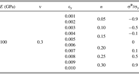
We considered a rigid spherical indenter penetrating into an infinite half-space with equibiaxial residual stress. Since it is an axisymmetric problem, an axisymmetric two-dimensional FE model was constructed in the commercial FE program ABAQUS29 to simulate the indentation response of linear elastic-power law strain hardening material with equibiaxial residual stress. The indenter was treated as an analytical rigid sphere with a radius of 100 μm, and the sample was modeled with 25,000 CAX4R elements which are composed of fine meshed elements near the contact region and gradually coarser meshed elements further from the contact region. For each simulation, the maximum indentation depth was fixed at 10 μm, i.e., h/R = 0.1. At the maximum indentation depth, the number of contact elements in the contact zone is about 150. The size of the sample was set to 2 × 2 mm which is about sixty times larger than the radius of the contact region, so that the sample can be regarded as an infinite half-space.Reference Myers, Knapp, Follstaedt and Dugger30,Reference Knapp, Follstaedt, Myers, Barbour and Friedmann31 The equibiaxial residual stress, σR, was simulated by applying pressure on the outer cylindrical surface of the sample prior to the indentation. Coulomb’s friction law was applied between the contact surfaces (with a friction coefficient of 0.15). To obtain the analytical expressions of dimensionless function, Πr, we considered a wide range of material parameters for commonly used metals. As listed in Table I, the yield strain, εy, ranges from 0.001 to 0.010 and takes 10 values, the strain-hardening exponent, n, ranges from 0.05 to 0.30 and takes 6 values, and the normalized equibiaxial residual stress, σR/σy, ranges from −0.9 to 0.90 (‘−’ indicates compression residual stress) and takes 7 values. Since the elastic modulus, E, does not influence the dimensionless function, it was fixed at 100 GPa for convenience. The combination of these parameters leads to 420 simulations which cover majority of the practical cases.
The mechanical parameters and residual stresses input into ABAQUS for simulations.

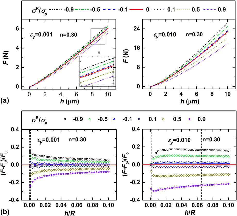
Typical indentation load–depth curves with different εy and σR/σy are shown in Fig. 1(a). It is clear that the loading curves are shifted upward by compressive residual stress and downward by tensile residual stress compared to the unstressed state. As the magnitude of residual stress decreases, the loading curve tends to move toward the one that does not display residual stress. In addition, the effect of the residual stress on the indentation loading curves becomes more significant for larger yield strain. Figure 1(b) shows the variation of (F − F 0)/F 0 with the normalized indentation depth, h/R, for different yield strains and equibiaxial residual stresses. As can be seen, the absolute value of (F − F 0)/F 0 decreases monotonically with the increase of the normalized indentation depth for a smaller yield strain (εy = 0.001), while for a larger yield strain (εy = 0.01), the absolute value of (F − F 0)/F 0 increases as the normalized indentation depth increases initially and decreases afterward. This could be explained by Eq. (15). When εy = 0.001, the normalized indentation depth range for the elastic–plastic transition regime is about from 5.4 × 10⁻⁶ to 6.6 × 10⁻⁴, and when εy = 0.01, the corresponding normalized indentation depth ranges approximately from 5.4 × 10⁻⁴ to 6.6 × 10⁻². The dashed lines in Fig. 1(b) display the normalized indentation depth range for the elastic–plastic transition regime. For εy = 0.001, the normalized indentation depth range for the elastic–plastic transition regime is rather narrow, and the fully plastic condition can be easily reached. For εy = 0.01, it has a comparatively wide range of indentation depth for elastic–plastic transition. It can be known from Eq. (11) that the initial indentation depth for the elastic–plastic transition regime is influenced by equibiaxial residual stress. Hence the maximum absolute value of (F − F 0)/F 0 appears at different normalized indentation depths in the elastic–plastic transition regime for different σR/σy as shown in the right part of Fig. 1(b). The absolute value of (F − F 0)/F 0 has a maximum value in the elastic–plastic transition regime and decreases continuously when the indentation depth exceeds this range. This agrees well with Taljat and Pharr’s findingReference Taljat and Pharr13 that the effect of equibiaxial residual stress on spherical indentation behaviors is significant in the elastic–plastic transition regime and becomes weaker in the fully plastic regime.
(a) The influence of equibiaxial residual stress on the indentation load–depth curves; (b) the variation of relative load difference with the normalized indentation depth.

To establish a method for evaluating equibiaxial residual stress based on Eq. (23), the equibiaxial residual stress should be related to the relative load difference, (F − F 0)/F 0, at a fixed h/R. It is evident from Fig. 1(b) that the equibiaxial residual stress has a most significant influence on the relative load difference in the elastic–plastic transition regime (i.e., the indentation depths between the two dotted lines). Using the maximum relative load difference in this regime to estimate the residual stress may have a favorable sensitivity. However, it is difficult to assign a fixed h/R in the elastic–plastic transition regime for all cases that the relative load difference reaches a maximum value. Moreover, the normalized indentation depths in the elastic–plastic transition regime are relatively small. Taking into account the actual situation that the tip of a spherical diamond indenter is not an ideal sphere due to the limitation of processing technology, it will introduce large measurement errors in load and depth at small normalized indentation depth. Thus, the relative load difference at the fixed normalized indentation depth of h/R = 0.1, where the relative load difference is more steady and accurate, was related to the equibiaxial residual stress.
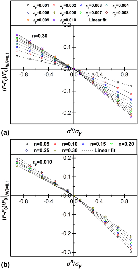
The correlations between (F − F 0)/F 0|h/R=0.1 and σR/σy for materials with a constant strain-hardening exponent of 0.3 and different yield strains are illustrated in Fig. 2(a). It clearly shows a bilinear relation between (F − F 0)/F 0|h/R=0.1 and σR/σy for compressive residual stress and tensile residual stress. And the slope of the plot of (F − F 0)/F 0|h/R=0.1 versus σR/σy decreases with increasing yield strain. Figure 2(b) shows the variation in (F − F 0)/F 0|h/R=0.1 with respect to σR/σy for materials with a constant yield strain of 0.1 and different strain-hardening exponents. These data also indicate an approximately linear relation between (F − F 0)/F 0|h/R=0.1 and σR/σy. The slopes of the plots of (F − F 0)/F 0|h/R=0.1 versus σR/σy are also different for compressive and tensile residual stresses. It can be concluded from Fig. 2 that (F − F 0)/F 0|h/R=0.1 varies linearly with σR/σy and the slope is a function of yield strain as well as strain-hardening exponent. Same conclusion could be derived from the FE results of other combinations of yield strain and strain-hardening exponent, which are not shown here due to the limitation of space. Based on this finding, Eq. (23) can be further simplified to
 $${\left. {{{F - {F_0}} \over {{F_0}}}} \right|_{h{\rm{/}}R = 0.1}} = {\left. {f\left( {{\varepsilon _{\rm{y}}},n} \right)} \right|_{h{\rm{/}}R = 0.1}}{{{\sigma ^{\rm{R}}}} \over {{\sigma _{\rm{y}}}}}\quad ,$$
where f(εy, n)|h/R=0.1 is the slope function, which is different for compressive residual stress and tensile residual stress.
The bilinear relation between the relative load difference at a normalized indentation depth of 0.1 and the normalized residual stress for materials (a) with a constant strain-hardening exponent of 0.3 and different yield strains; (b) with a constant yield strain of 0.1 and different strain-hardening exponents.

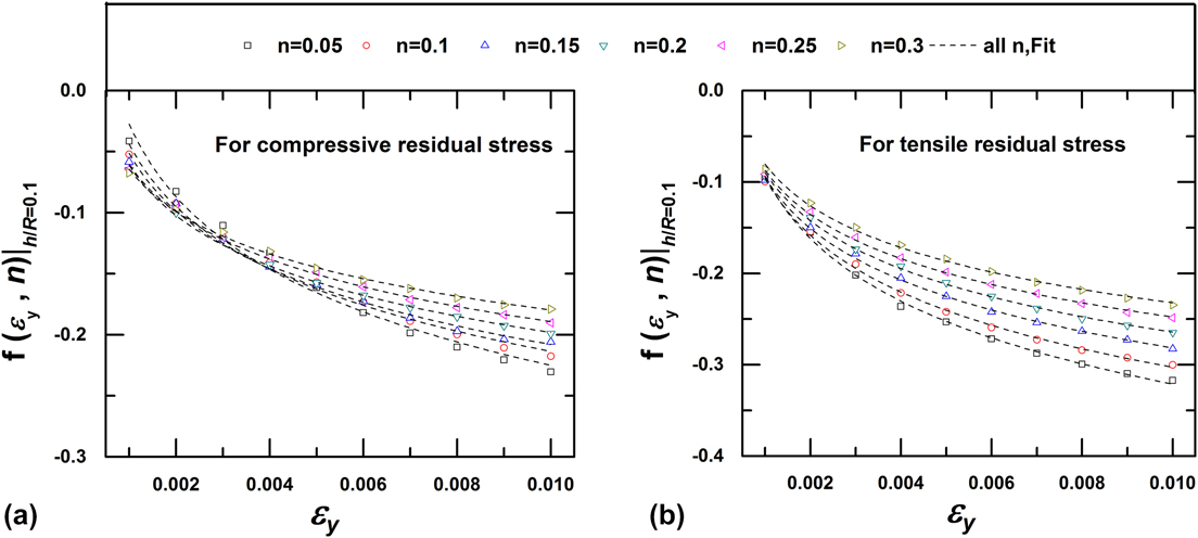
We plotted the slope versus the yield strain in Figs. 3(a) and 3(b), respectively, for compressive residual stress and tensile residual stress. By fitting a logarithmic equation, f(εy, n)|h/R=0.1 = g 1(n)lg(εy) + g 2(n), to the data points in Figs. 3(a) and 3(b), respectively, the slope function was evaluated. For compressive residual stress, i.e., (F − F 0) > 0, the slope function is
 $$\matrix{ {{{\left. {{f_{\rm{c}}}\left( {{\varepsilon _{\rm{y}}},n} \right)} \right|}_{h{\rm{/}}R = 0.1}} = \left( { - 0.66535{n^2} + 0.54962n - 0.22177} \right)\lg \left( {{\varepsilon _{\rm{y}}}} \right)} \cr { - 1.30556{n^2} + 1.26769n - 0.67626} \cr} \quad .$$
The effects of the strain hardening exponent and the yield strain on the evolution of the slope function for (a) compressive residual stress and (b) tensile residual stress. Dashed lines are the best-fitting curves to the data points of the same strain hardening exponent.

For tensile residual stress, i.e., (F − F 0) < 0, the slope function becomes
 $$\matrix{ {{{\left. {{f_{\rm{t}}}\left( {{\varepsilon _{\rm{y}}},n} \right)} \right|}_{h{\rm{/}}R = 0.1}} = \left( { - 0.61027{n^2} + 0.51775n - 0.25209} \right)\lg \left( {{\varepsilon _{\rm{y}}}} \right)} \cr { - 1.45435{n^2} + 1.47543n - 0.84722} \cr} \quad .$$
Thus far, the analytical equation relating the equibiaxial residual stress to the indentation parameter, (F − F 0)/F 0|h/R=0.1, has been established as
 $${{{\sigma ^{\rm{R}}}} \over {{\sigma _{\rm{y}}}}} = \left\{ {\matrix{ \matrix{ \left[ {\left( { - 0.66535{n^2} + 0.54962n - 0.22177} \right)} \right.\lg \left( {{\varepsilon _{\rm{y}}}} \right) \hfill \cr {\left. { - 1.30556{n^2} + 1.26769n - 0.67626} \right]^{ - 1}}{\left. {{{F - {F_0}} \over {{F_0}}}} \right|_{h/R = 0.1}} \hfill \cr} & {{\rm{\ for}}\;\left( {F - {F_0}} \right) > 0} \cr \matrix{ \left[ {\left( { - 0.61027{n^2} + 0.51775n - 0.25209} \right)} \right.\lg \left( {{\varepsilon _{\rm{y}}}} \right) \hfill \cr {\left. { - 1.45435{n^2} + 1.47543n - 0.84722} \right]^{ - 1}}{\left. {{{F - {F_0}} \over {{F_0}}}} \right|_{h/R = 0.1}} \hfill \cr} & {{\rm{for}}\;\left( {F - {F_0}} \right) \lt 0} \cr} \quad ,} \right.$$
which can be used to calculate the equibiaxial residual stress if the elastic–plastic parameters, E, εy, and n, are known.
E. Integrated method
In our previous work,Reference Yu, Feng, Yang, Peng, Lu and Zhang24 a method has been proposed to determine the elastic–plastic parameters of linear elastic-power law strain hardening materials using instrumented spherical indentation. The formulae for calculating the elastic modulus, the yield strain, and strain-hardening exponent are given as
 $$\left\{ {\matrix{ {{W_{\rm{t}}} = {{2\pi E\varepsilon _{\rm{y}}^2{c^3}} \over {3n\left( {n + 1} \right)}}\left( {{{{c^{3n}}} \over {{b^{3n}}}} - 1} \right) + {{\left( {n - 1} \right)\pi E\varepsilon _{\rm{y}}^2{b^3}} \over {3\left( {n + 1} \right)}}\left( {{{{c^3}} \over {{b^3}}} - 1} \right) + {{\pi E\varepsilon _{\rm{y}}^2{c^3}} \over 3}} \hfill \cr {{W_{\rm{u}}} = {{\pi \left( {1 + \nu } \right)E\varepsilon _{\rm{y}}^2{b^3}} \over 2}\left[ {\left( {242.62{\varepsilon _{\rm{y}}} - 4.6663} \right){n^2} + \left( { - 268.30{\varepsilon _{\rm{y}}} + 3.1253} \right)n} \right.} \hfill \cr {\left. { + \left( {57.053{\varepsilon _{\rm{y}}} + 0.56730} \right)} \right]{{\left[ {{{\left( {{{7 - 8\nu } \over 3}} \right)}^n}{2 \over {3n}}\left( {{{{c^{3n}}} \over {{b^{3n}}}} - 1} \right) + 1} \right]}^2}} \hfill \cr {m = \left( { - 70.436{\varepsilon _{\rm{y}}} + 2.1866} \right)n + \left( {49.355{\varepsilon _{\rm{y}}} + 1.8547} \right)} \hfill \cr} \quad ,} \right.$$
where the total work, W t, the unloading work, W u, and the Meyer’s coefficient, m, can be obtained directly from the indentation load–depth curve; b and c are the radii of the hemispherical hydrostatic core and the hemispherical hydrostatic plastic zone, respectively, in the Johnson’s expanding cavity model.Reference Johnson26 These radii are described by
 $$b = \sqrt {2Rh - {h^2}} \quad ,$$
and
 $$\matrix{ {c = \left[ {\left( { - 0.0077{n^2} + 0.0534n - 0.0304} \right){{\lg }^2}\left( {{\varepsilon _{\rm{y}}}} \right)} \right.} \cr { + \left( {0.3717{n^2} - 0.1331n - 0.0774} \right)\lg \left( {{\varepsilon _{\rm{y}}}} \right)} \cr {\left. { + \left( {0.4950{n^2} - 0.3016n + 1.0627} \right)} \right]{{\left[ {{{{h^2}\left( {3R - h} \right)} \over {3{\varepsilon _{\rm{y}}}}}} \right]}^{1{\rm{/}}3}}} \cr} \quad .$$
Based on Eqs. (27) and (28), an integrated method for evaluating the elastic–plastic parameters and the equibiaxial residual stress was developed. Specifically, the first step is to carry out spherical indentation tests on unstressed sample with a maximum depth of h/R = 0.3 and on stressed sample with a depth of h/R > 0.1. The second step is to obtain W t, W u, and m from the unstressed load–depth curve by fitting and obtain (F − F 0)/F 0|h/R=0.1 by comparing the stressed load–depth curve with unstressed load–depth curves at the depth of h/R = 0.1. The final step is to substitute W t, W u, m, and (F − F 0)/F 0|h/R=0.1 into Eqs. (27) and (28) to calculate the elastic–plastic parameters and the equibiaxial residual stress simultaneously.
III. EXPERIMENTS
Both uniaxial tensile tests and indentation tests were carried out on three commonly used metals (Al 2024, Al 7075, and Ti Grade 5). The indentation results will be compared with the corresponding uniaxial tensile results to verify the validity and reliability of the newly proposed method.
A. Specimens
For uniaxial tensile tests, the 3-mm-thick Al 2024, Al 7075, and Ti Grade 5 plates were processed into dumbbell-shaped specimens according to ISO 6892-1. For instrumented indentation tests, these plates were cut into dumbbell-shaped specimens with a cross-section measuring 4 × 3 mm (see Fig. 4). The surfaces of specimens for indentation tests were polished to mirror finish surfaces using an automatic polishing machine with 0.3 μm alumina powder. All the Al 2024 and Al 7075 specimens were annealed at 180 °C and Ti Grade 5 were annealed at 480 °C for 10 h to relieve the residual stress caused by mechanical processing.
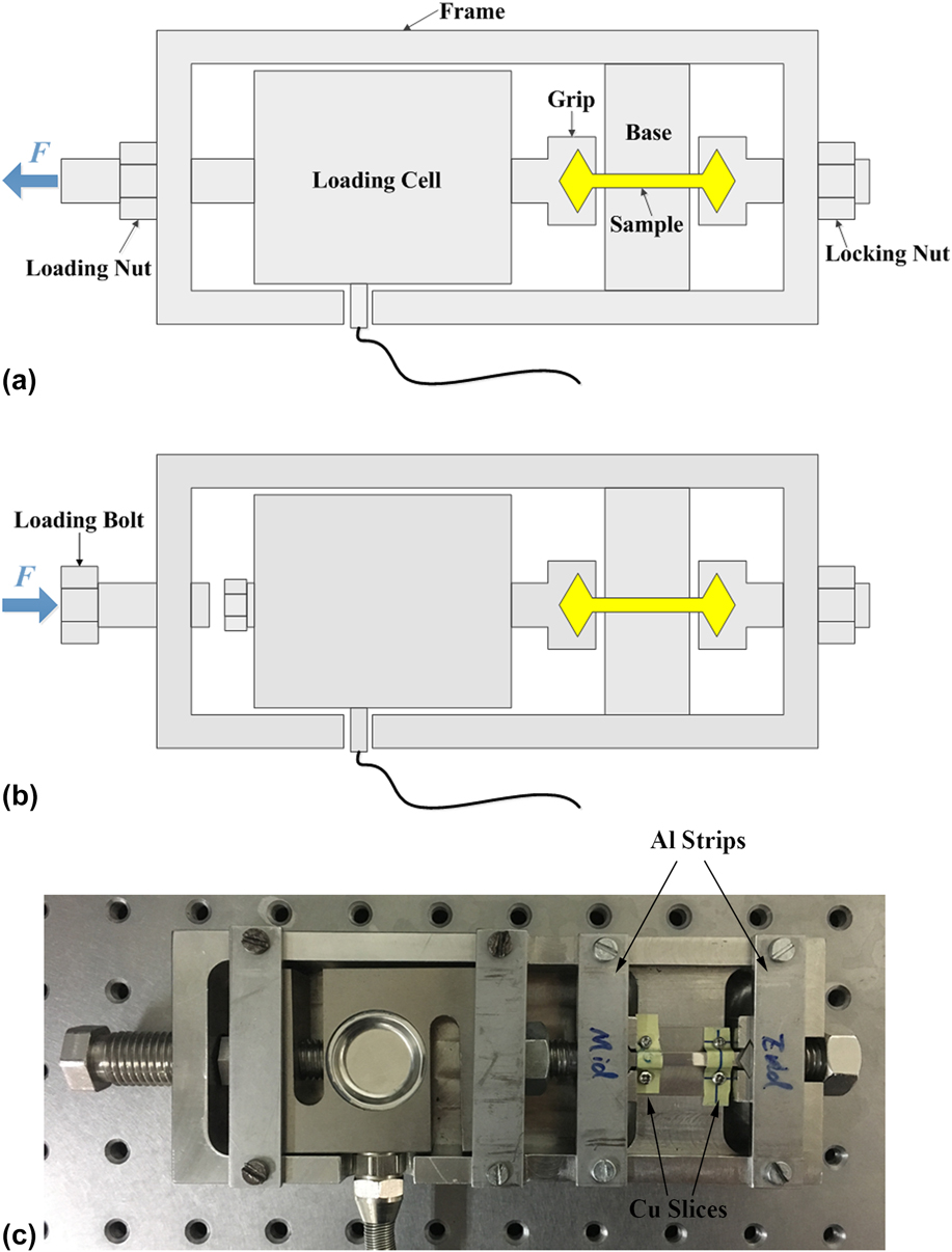
Schematic diagram of the residual stress-generating jig for (a) tensile stress and (b) compressive stress; (c) photograph of the jig for generating compressive stress.

B. Uniaxial tensile tests
A material testing system MTS 810 (MTS, Minneapolis, MN) was used to perform uniaxial tensile tests on Al 2024, Al 7075, and Ti Grade 5 at room temperature according to ISO 6892-1. Uniaxial tensile tests were performed in a displacement-controlled manner, and the displacement increased at a constant extension rate of 5 mm/min. The elastic modulus, yield strain as well as strain-hardening exponent determined by uniaxial tension are regarded as the reference values.
C. Instrumented indentation tests
Instrumented spherical indentation tests were carried out on three metals at room temperature using a universal hardness testing machine (ZHU2.5/Z2.5, Zwick/Roell Corporation, Ulm-Einsingen, Germany) with a spherical diamond indenter whose nominal radius is 90 μm. Since the radius of the indenter plays a very important role in the results analysis, the three-dimensional observation of the indenter tip was performed using a confocal laser scanning microscope (OLS4000, OLYMPUS, Shinjuku Monolith, Tokyo, Japan), which has a vertical resolution of 0.01 μm and a horizontal resolution of 0.12 μm.
A residual stress-generating jig illustrated in Fig. 4 was designed to control the stress in the specimen by screwing in a loading nut for tension or a loading bolt for compression. To avoid buckling when compressive stress was applied, two aluminous strips and two cupreous slices were used to constrain the out-of-plane displacement of the specimen as shown in Fig. 4(c). Specifically, to generate compressive stress, there are 5 steps: (i) putting the dumbbell-shaped specimen into the grips and making sure that the lower surface fully touches the support table of the jig. (ii) Using Cu slices to fix the specimen on the support table and Al strips to cover both ends of the specimen to constrain the out-of-plane displacement. (iii) Screwing in the loading bolt carefully to compress the specimen without bending. (iv) Checking and making sure that the specimen is not bent and there is no gap between specimen and support table [If bent, repeat steps (i)–(iv)]. (v) Cleaning the top surface of the specimen and getting ready for indentation tests. During the test processes, the stress-generating jig was fixed on the sample stage by glues to eliminate the gap between the jig and the sample stage. Following these procedures, the frame compliance could be reduced to a minimum. The load exerted on the specimen was measured by a load cell (here, the friction force between the cupreous slices and the specimen was ignored), and the applied stress can then be calculated (the applied load divided by the specimen’s cross-sectional area 4 × 3 mm). For each type of metal, five levels of uniaxial stress (one stress-free state, two tensile stress states, and two compressive stress states) were exerted on the specimens to imitate different residual stresses. For each stress state, indentation tests were repeated 5 times. The maximum indentation depth was set to about 0.3R for stress-free specimens and greater than 0.1R for stressed specimens.
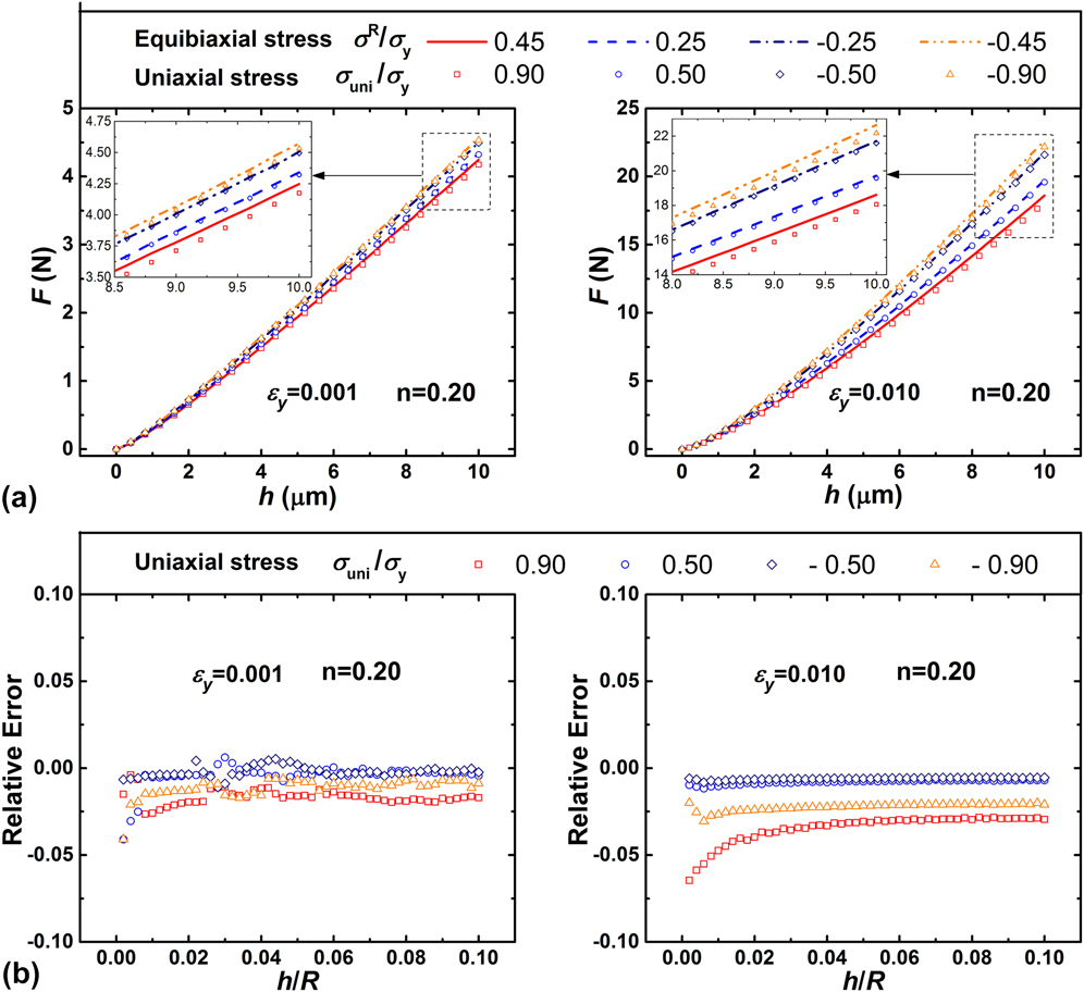
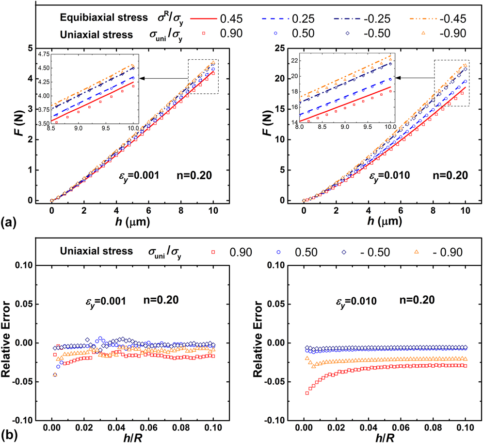
In the spherical indentation tests, uniaxial stress was introduced instead of equibiaxial stress. To demonstrate the feasibility of replacing equibiaxial stress with uniaxial stress, three-dimensional FE models with equibiaxial residual stress and uniaxial residual stress were carried out in the commercial FE program ABAQUS.29 The indenter parameters, indentation depth, and material parameters are the same as used in Sec. II.D. Based on Giannakopoulos’sReference Giannakopoulos32 argument that the equibiaxial residual stress is equivalent to the half value of the uniaxial stress for sharp indentation, four levels of normalized uniaxial residual stress (σuni/σy = 0.90, 0.50, −0.50, −0.90) and normalized equibiaxial residual stress (σR/σy = 0.45, 0.25, −0.25, −0.45) were considered to verify that this argument is also applicable for spherical indentation. The comparison between indentation load–depth curves with uniaxial stress and these with equibiaxial stress is illustrated in Fig. 5. It clearly shows that the load–depth curve of the uniaxial stressed sample approximately coincides with that of the equibiaxial stressed sample with half-value stress. The relative error increases with the increasing of residual stress and yield strain of the sample. For εy = 0.01 and n = 0.20, the maximum relative error at normalized indentation depth, h/R = 0.1, is within 3%. It can be concluded from the current computing results that the equibiaxial stress can be approximately replaced with uniaxial stress in spherical indentation tests if the applied uniaxial stress does not exceed 0.9σy and the sample’s yield strain is no more than 0.01.
(a) Comparison between indentation load–depth curves of the uniaxial stressed sample and those of the equibiaxial stressed sample with half-value stress; (b) the relative error between them at different normalized indentation depths.
IV. RESULTS AND DISCUSSION
A. Indenter shape
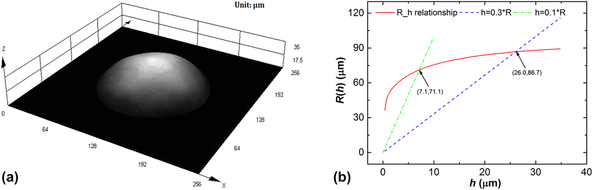
The observation result of the spherical indenter used in the indentation tests is shown in Fig. 6(a). It clearly shows that the diamond indenter tip is not an ideal sphere and the curvature of the surface varies with the indenter latitude. To improve the accuracy of data analysis, the equivalent radii of the spherical indenter at different indentation depths were evaluated according to the volume conservation condition. It is considered that if the actual spherical indenter tip has the same volume as an ideal spherical indenter tip does at the same depth, h i, the actual spherical indenter’s equivalent radius at h i is equal to the ideal spherical indenter’s radius. The volume of an ideal spherical indenter tip at the depth, h i, can be expressed as
 $$V\left( {{h_{\rm{i}}}} \right) = \pi h_{\rm{i}}^2\left[ {R\left( {{h_{\rm{i}}}} \right) - {{{h_{\rm{i}}}} \over 3}} \right]\quad .$$
(a) The geometrical surface of the spherical indenter tip measured by OLYMPUS OLS4000; (b) the equivalent radii of the spherical diamond indenter at various depths (solid line). The arrows mark the equivalent radii at h/R = 0.1 and h/R = 0.3.

Thus, the radius of the ideal spherical indenter, R(h i), which is also regarded as the equivalent radius of the actual spherical indenter, is given as
 $$R\left( {{h_{\rm{i}}}} \right) = {{V\left( {{h_{\rm{i}}}} \right)} \over {\pi h_{\rm{i}}^2}} + {{{h_i}} \over 3}\quad .$$
When the volume of the actual spherical indenter tip, V(h i), at various depths was measured from the 3D observation data [see Fig. 6(a)], the equivalent radius, R(h i), at various depths can be calculated by Eq. (32). It can be found from Fig. 6(b) that the equivalent radius increases with the increasing depth. The equivalent radius of the actual spherical indenter is about 71.1 μm at the depth, h i = 0.1R, and about 86.7 μm at the depth, h i = 0.3R.
B. Elastic–plastic parameters
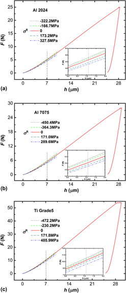
The indentation load–depth curve without residual stress (see the solid curve in Fig. 7) was used to determine the elastic–plastic parameters by Eq. (28). For each material, the values of the total work, W t, the unloading work, W u, and the Meyer’s coefficient, m, were obtained directly from the load–depth curve by integrating and fitting. Then, substituting W t, W u, and m into Eq. (28), the elastic modulus, the yield strength, and the strain-hardening exponent were calculated. Here, the mean value of the elastic modulus,  ${\bar{E}_0}$, the yield strength,
 ${\bar{\sigma }_{{\rm{y}}0}}$, and the strain-hardening exponent,
 ${\bar{n}_0}$, measured by uniaxial tension were conventionally regarded as the reference values. As listed in Table II, the mean values of the elastic–plastic parameters determined by the proposed method were compared with the corresponding uniaxial tensile results. For all three materials, the maximum relative error of the elastic modulus is within ±15% and that of the yield strength is within ±10%. This indicates that the indentation results have a good agreement with the uniaxial tensile results.
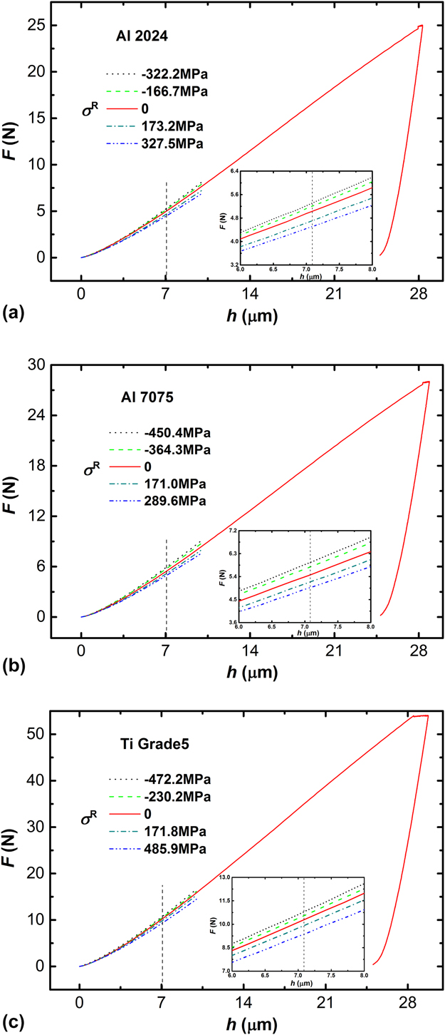
The resulting mean load–depth curves of five indentations in each stress state for (a) Al 2024, (b) Al 7075, and (c) Ti Grade 5.

The mean value of elastic–plastic parameters determined by uniaxial tensile tests and instrumented indentation tests.

C. Residual stress
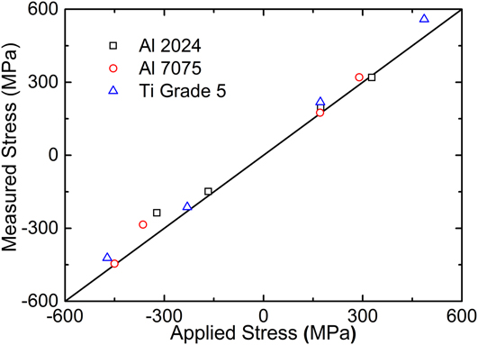
The spherical indentation load–depth curves of samples with and without residual stress are shown in Fig. 7. Since the equivalent radius of the spherical indenter is about 71.1 μm, the indentation depth equals 7.1 μm at the normalized indentation depth of h/R = 0.1. The relative load difference, (F − F 0)/F 0|h/R=0.1, were then obtained by comparing the indentation loads of the stressed and unstressed samples at the depth of 7.1 μm. Substituting (F − F 0)/F 0|h/R=0.1 and the above determined elastic–plastic parameters into Eq. (27), the equibiaxial residual stress were calculated. Because the equibiaxial residual stress is equivalent to the half value of the uniaxial stress as GiannakopoulosReference Giannakopoulos32 argued, the uniaxial stress should be twice the value calculated by Eq. (27). Figure 8 clearly shows that the residual stresses estimated by the newly proposed method agree well with the applied stresses in a wide range of stresses. The relative errors between the estimated stresses and the applied stresses are commonly within ±20%. This demonstrates that the newly proposed method is a reliable method for estimation of the equibiaxial residual stress in metals.
Comparison of the measured residual stresses and the applied stresses.

Based on Eq. (27), applying error analysis leads to
 $${{\Delta {\sigma ^{\rm{R}}}} \over {{\sigma ^{\rm{R}}}}} = \left\{ {\matrix{ {{{\Delta E} \over E} + \left( {1 + {{\lg e} \over {\lg {\varepsilon _{\rm{y}}}}}} \right){{\Delta {\sigma _{\rm{y}}}} \over {{\sigma _{\rm{y}}}}} + {k_1}{{\Delta n} \over n} + {{\Delta {F_{\rm{D}}}} \over {{F_{\rm{D}}}}},} & {{\rm{for}}\;\left( {F - {F_0}} \right) > 0} \cr {{{\Delta E} \over E} + \left( {1 + {{\lg e} \over {\lg {\varepsilon _{\rm{y}}}}}} \right){{\Delta {\sigma _{\rm{y}}}} \over {{\sigma _{\rm{y}}}}} + {k_2}{{\Delta n} \over n} + {{\Delta {F_{\rm{D}}}} \over {{F_{\rm{D}}}}},} & {{\rm{for}}\;\left( {F - {F_0}} \right) \lt 0} \cr} } \right.\quad ,$$
where
 $$\left\{ {\matrix{ \matrix{ {k_1} = \left[ {\left( { - 0.66535{n^2} + 0.54962n - 0.22177} \right)} \right.\lg \left( {{\varepsilon _{\rm{y}}}} \right){\left. { - 1.30556{n^2} + 1.26769n - 0.67626} \right]^{ - 1}} \hfill \cr \times \left[ {\left( { - 1.33070{n^2} + 0.54962n} \right)\lg \left( {{\varepsilon _{\rm{y}}}} \right) - 2.61112{n^2} + 1.26769n} \right] \hfill \cr} \hfill \cr \matrix{ {k_2} = \left[ {\left( { - 0.61027{n^2} + 0.51775n - 0.25209} \right)} \right.\lg \left( {{\varepsilon _{\rm{y}}}} \right){\left. { - 1.45435{n^2} + 1.47543n - 0.84722} \right]^{ - 1}} \hfill \cr \times \left[ {\left( { - 1.22054{n^2} + 0.51775n} \right)} \right.\lg \left( {{\varepsilon _{\rm{y}}}} \right)\left. { - 2.90870{n^2} + 1.47543n} \right] \hfill \cr} \hfill \cr {{F_{\rm{D}}} = {{\left. {{{F - {F_0}} \over {{F_0}}}} \right|}_{h/R = 0.1}}} \hfill \cr {e = 2.71828} \hfill \cr} } \right.\quad .$$
From Eq. (33), it clearly shows that errors in the elastic modulus, the yield strength, the strain-hardening exponent, and the relative load difference contribute directly to the error of estimated stress. Since the value of yield strain is typically range from 0.001 to 0.010, (1 + lg e/lg εy) ranges from 0.78285 to 0.85526. This means that the contribution of the error in yield strength to the error of estimated stress shrinks. Substituting the parameters of Al 2024, Al 7075, and Ti grade 5 presented in Table II into Eq. (34), it could be calculated that k 1 ranges from −0.10092 to −0.03161 and k 2 ranges from −0.20581 to −0.06990. This means that the estimated stress is insensitive to the error in strain-hardening exponent.
V. CONCLUSIONS
An integrated method that can be used to effectively estimate the surface equibiaxial residual stress as well as the elastic–plastic parameters of metals was proposed. This method neither needs measurement of the actual contact area nor requires the materials’ elastic–plastic parameters to be known in advance. Applications were illustrated on three commonly used metals (Al 2024, Al 7075, and Ti Grade 5) with various stresses applied by a stress-generating jig. The maximum relative error between the values determined by this integrated method and the reference values is generally within ±10% for the yield strength, within ±15% for the elastic modulus and within ±20% for the equibiaxial residual stress. It thus demonstrates that the newly proposed method is valid and reliable for estimation of the equibiaxial residual stress and elastic–plastic properties of metals simultaneously via instrumented spherical indentation.
VI. PROSPECTS
In engineering, engineers sometimes need to know the stress state in large engineering structures such as spherical pressure vessels and oil pipelines when they are in service. Typically, the stresses in spherical pressure vessels are approximately regarded as equibiaxial residual stresses and the main stress in pipelines is hoop stress which can be equivalent to uniaxial stress in a small area. In such cases, our newly proposed method in alliance with a portable instrumented indentation machine could be a nondestructive and promising technique for estimating the stresses in spherical pressure vessels and oil pipelines when they are in service.
ACKNOWLEDGMENTS
The authors would like to gratefully acknowledge the support from the National Natural Science Foundation of China (Grant Nos. 11727803, 11772302, 11672356, 11502235, and 11402233) and Public Welfare Project of Zhejiang Province (2015C31074).