


I. INTRODUCTION
A demand in increasing bandwidth has driven researchers to explore waveguides as high-speed data communication channels [Reference Yeh, Shimabukuro and Siegel1–Reference Song, Jin and Bae5]. Especially, a coherent optical fiber/waveguide communication has shown tremendous potential in scaling bandwidth because of its capabilities of in-phase/quadrature-phase and multi-level signaling [Reference Kikuchi6].
Waveguides are known to be dispersive or band-limited because of non-linear propagation constant (β), and bandwidth capacity is traditionally estimated through a group delay (τ g) variation [Reference Kapron and Keck7]. Assuming a narrow input data bandwidth (BW) is applied through a waveguide, a group delay and pulse broadening coefficient (τ p) at a target carrier frequency (ω 0) is expressed as,
 $$\tau _g = \left. {\displaystyle{{d\beta} \over {d\omega}}} \right \vert _{\omega = \omega _0}({\rm s}/{\rm m}),$$
 $$\tau _p = BW \times \left. {\displaystyle{{d\tau _g} \over {d\omega}}} \right \vert _{\omega = \omega _0} = BW \times \left. {\displaystyle{{d^2\beta} \over {d^2\omega}}} \right \vert _{\omega = \omega _0}({\rm s}/{\rm m}),$$
where ω is an angular frequency. As indicated in (2), the larger the bandwidth, the higher pulse broadening will be added to an originally transmitted pulse over distance. From an input baseband pulse point of view in time domain, a first-order derivative of β simply delays, second-order derivative delays and broadens; from third-order and beyond, it delays, broadens, and distorts all together. As a communication bandwidth enters regimes much greater than multi-tens of gigabits per second (>10 Gb/s), a group delay variation method not only violates a narrow bandwidth assumption, but it also completely neglects a distortion and ISI effect.
In this paper, an impulse response analysis is introduced to analyze baseband data behavior through waveguides under a coherent communication system. The goal of this paper is to provide a comprehensive understanding of waveguide communication depending on the bandwidth of baseband data, carrier frequency, phase mismatch, and propagation mode through time domain simulations instead of group delay estimation. According to Maxwell's equations, an input to output relationship of waveguide is categorized as a linear time-invariant (LTI) system. In other words, if an impulse response of waveguide is known, an output can be calculated for any given input data pattern [Reference Kim, Cho, Du, Cong, Itoh and Chang8]. Accordingly, the first step to design a high-speed communication system is to typically determine the impulse response of a given channel [Reference Azadet9–Reference Gondi and Razavi11]. Although there have been attempts to characterize impulse response of waveguides, they require either direct measurements or again narrow bandwidth assumption to linearize a propagation constant [Reference Gloge12–Reference Chatterjee and Green15]. Instead, borrowing concepts from communication theory, a frequency domain convolution and multiplication method is applied by taking both negative and positive frequency regions into considerations. The proposed analysis achieves an exact expression of baseband equivalent impulse response in frequency domain and leads to a true impulse response in time domain by way of an inverse Fourier transform. As long as frequency-dependent attenuation (σ) and propagation constant (β) is provided, the analysis can be applied to any shape (rectangular, circular, elliptical) or any type (dielectric, metallic) of waveguide in an arbitrary frequency range. A dielectric-filled metallic circular waveguide and air-filled metallic rectangular waveguide is presented as examples since they offer σ and β in closed-form equations.
II. BASEBAND EQUIVALENT IMPULSE RESPONSE
A coherent detection-based full system diagram is illustrated in Fig. 1(a). By splitting a signal vector space, namely in-phase and quadrature-phase, a coherent architecture can achieve an enhanced bandwidth efficiency with modulation schemes such as quadrature-phase shift keying and 16-quadrature amplitude shift keying [Reference Cho16, Reference Cho17]. The system diagram in Fig. 1 contains only an in-phase path, but a quadrature path could always be applied when necessary.
(a) Coherent-based full transmitter and receiver system includes up-converter, down-converter, local oscillators, and low-pass filter. Two local oscillators are assumed to be phase and frequency synchronized in the transmitter and receiver side. (b) The full system is replaced by a baseband equivalent waveguide channel as an impulse response.
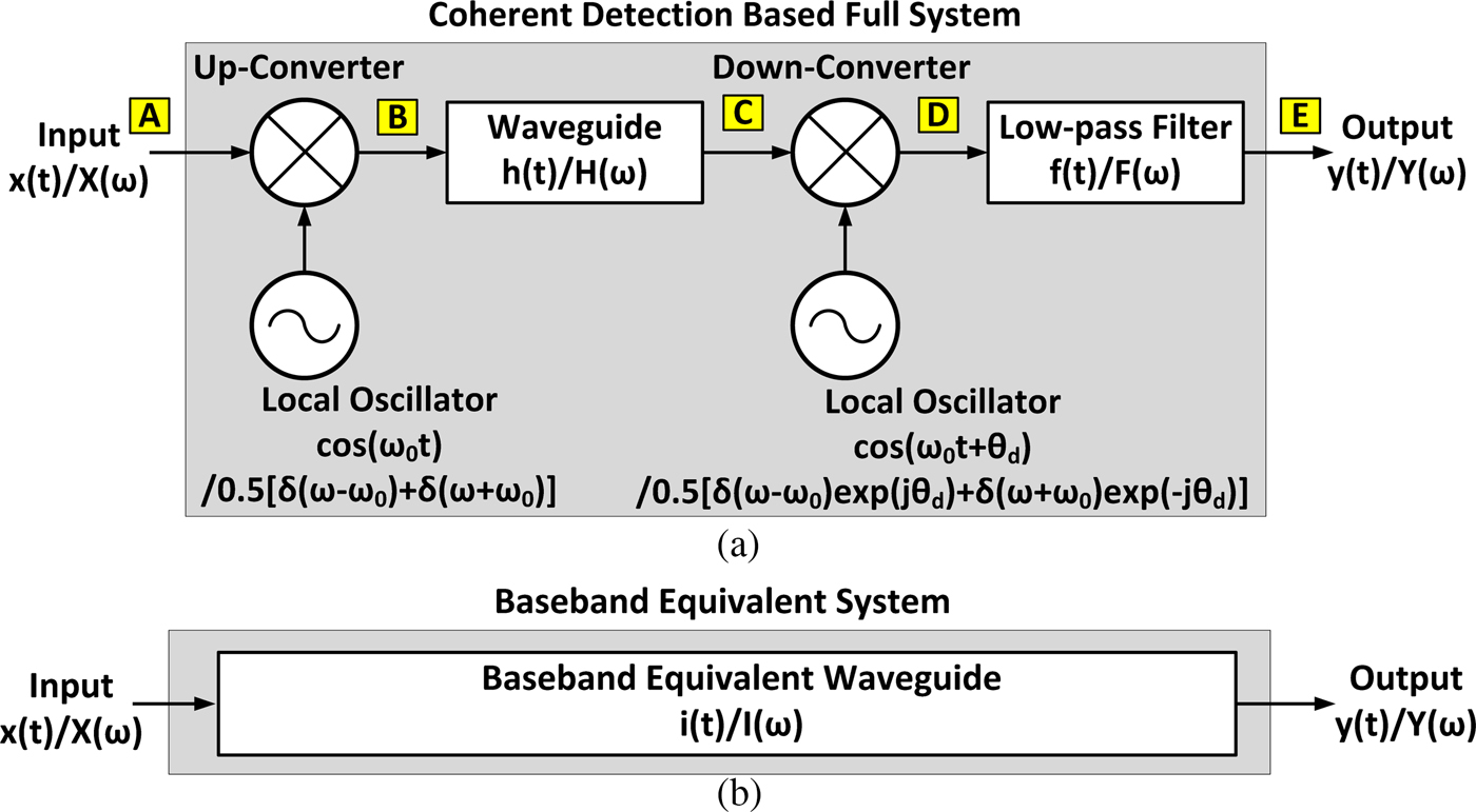
In the diagram, time domain and frequency domain symbols are written with lower case and upper case letters, respectively. An input data x(t) modulates a carrier (ω 0) via an up-converter and travels through a waveguide h(t). A down-converter then de-modulates an incoming signal with a receiver side local oscillator (LO). A fixed amount of extra LO phase, which is directly calculated from a waveguide channel delay at a carrier frequency, is added to a receiver LO to synchronize a phase between transmitter and receiver. A method of synchronization is beyond the discussion of this paper, and they are assumed to be synchronized (a consequence will be explained if not synchronized). In the last stage, a low-pass filter (LPF) filters out the residue of 2ω 0 component generated from the down-conversion process. An ultimate goal is to capture the non-linear property of waveguide propagation constant and translate into a baseband equivalent impulse response i(t) or I(ω) model as in Fig. 1(b). With an impulse response defined, an output becomes,
 $$Y(\omega ) = X(\omega )I(\omega ),$$
 $$y(t) = x(t)*i(t),$$
where * operator indicates a convolution.
Based on the system block diagram, the process of frequency domain computation is built in Fig. 2. After solving boundary conditions of a given waveguide, a frequency response (or commonly referred as a time-harmonic expression) of electromagnetic field propagating in z-direction can be readily characterized as,
 $$H_ + \left( \omega \right) = \left\{ \matrix{ e^{ - \alpha (\omega )z}e^{ - j\beta (\omega )z} &(\omega \gt 0) \cr \hskip-4.3pc 0 &(\omega \lt 0)} \right.$$
 $$H_ - \left( \omega \right) = \left\{ \matrix{\hskip-4.3pc 0 &(\omega \gt 0) \cr e^{ - \alpha (\omega )z}e^{ + j\beta (\omega )z} &(\omega \lt 0)} \right.$$
 $$H(\omega ) = H_ + (\omega ) + H_ - (\omega ),$$
where z is the length of wave traveled [Reference Pozar18]. H(ω) splits into (+) and (−) components to handle a conjugate symmetric property of frequency response. An attenuation constant α and propagation constant β is frequency-dependent, geometry-dependent, waveguide-type-dependent, and mode-dependent. To demonstrate this idea, an input spectrum X(ω) and waveguide frequency response H(ω) are configured arbitrarily in Fig. 2. A key message in this figure is to include and calculate a negative frequency spectral portion throughout the process. To summarize the process at each node,
 $$A:X(\omega ),$$
 $$TX{\rm} \; LO:\displaystyle{1 \over 2}\left[ {\delta {\rm (}\omega + \omega _0{\rm )} + \delta {\rm (}\omega - \omega _0{\rm )}} \right],$$
 $$B:\displaystyle{1 \over 2}\left[ {X(\omega + \omega _0) + X(\omega - \omega _0)} \right],$$
 $$C:\displaystyle{1 \over 2}\left[ {X(\omega + \omega _0)H_ - (\omega ) + X(\omega - \omega _0)H_ + (\omega )} \right],$$
 $$\eqalign{& RX \; {\rm} LO:\displaystyle{1 \over 2}\left[ {\delta {\rm (}\omega + \omega _0{\rm )}e^{ + j\beta (\omega )z} + \delta {\rm (}\omega - \omega _0{\rm )}e^{ - j\beta (\omega )z}} \right] \cr & \quad = \displaystyle{1 \over 2}\left[ {\delta {\rm (}\omega + \omega _0{\rm )}e^{ + j\beta ( - \omega _0)z} + \delta {\rm (}\omega - \omega _0{\rm )}e^{ - j\beta (\omega _0)z}} \right],} $$
 $$\eqalign{& \; D:\left\{ {\displaystyle{1 \over 2}\left[ {X(\omega + \omega _0)H_ - (\omega ) + X(\omega - \omega _0)H_ + (\omega )} \right]} \right\} \cr & \qquad \quad *\left\{ {\displaystyle{1 \over 2}\left[ {\delta (\omega + \omega _0)e^{ + j\beta ( - \omega _0)z} + \delta (\omega - \omega _0)e^{ - j\beta (\omega _0)z}} \right]} \right\}.} $$
In (10), only a fixed phase portion is extracted from H(ω) and accumulated to a receiver LO for phase synchronization. Next, (11) can be further expanded to,
 $$\eqalign{&\displaystyle{1 \over 4}X(\omega )\left[ {H_ - (\omega - \omega _0)e^{ - j\beta (\omega _0)z} + H_ + (\omega + \omega _0)e^{ + j\beta ( - \omega _0)z}} \right] \cr & \qquad \qquad + \displaystyle{1 \over 4}X(\omega + 2\omega _0)H_ - (\omega + \omega _0)e^{ + j\beta ( - \omega _0)z} \cr & \qquad \qquad + \displaystyle{1 \over 4}X(\omega - 2\omega _0)H_ + (\omega - \omega _0)e^{ - j\beta (\omega _0)z}.}$$
The first term in (12) discloses that a baseband spectrum is multiplied by a sum of two frequency-shifted waveguide channel responses. For the latter two terms, it is clear that they are 2ω 0 components, and they make the system in (12) linear time-variant. Thus, from a mathematical standpoint, an LPF must fully reject the 2ω 0 residue in order for a baseband equivalent frequency response to remain as an LTI system. Practically speaking, the above statement is a reasonable assumption, for instance, if a carrier frequency is 100 GHz, a residue will appear at 200 GHz, which can be easily filtered out even with a one-pole LPF. Therefore, an output spectrum can be written as,
 $$\eqalign{ E:Y(\omega ) & = \displaystyle{1 \over 4}X(\omega )F(\omega ) \cr & \times \left[ {H_ - (\omega - \omega _0)e^{ - j\beta (\omega _0)z} + H_ + (\omega + \omega _0)e^{ + j\beta ( - \omega _0)z}} \right].} $$
A choice of LPF could greatly affect a baseband equivalent impulse response. In order not to be dominated by a filter frequency response, only a simple one-pole R and C filters with tens of pico-seconds (ps) time constant will be used. Following the definition of impulse response, x(t) = δ(t), which is X(ω) = 1, can be inserted to (13), and finally a baseband equivalent impulse response in frequency domain is derived as,
 $$\! \eqalign{ I(\omega ) & = \left. {Y(\omega )} \right \vert _{X\left( \omega \right) = 1} \cr & = \displaystyle{1 \over 4}F(\omega ) \left[ {H_ - (\omega - \omega _0)e^{ - j\beta (\omega _0)z} + H_ + (\omega + \omega _0)e^{ + j\beta ( - \omega _0)z}} \right].} $$
There are two important things to highlight. First, a baseband equivalent impulse response in frequency domain consists of positively shifted and negatively shifted H(ω) around a carrier frequency. Second, an impulse response depends on a carrier frequency. For example, with a given geometry, dimension, and length of waveguide, as a carrier frequency increases, a modulated wave propagates closer to a transverse electromagnetic (TEM)-like mode, expecting less dispersion and distortion. So far, a mathematical framework has been developed. In-depth analysis with examples will deliver intuition in the following chapters.
The process of frequency domain calculation is shown in alphabetical order that was listed in Fig. 1(a). Note from the property of LTI system that time domain multiplication becomes frequency domain convolution, and time domain convolution becomes frequency domain multiplication.

III. DIELECTRIC-FILLED METALLIC CIRCULAR WAVEGUIDE
Propagation properties of metallic circular waveguide are well defined with closed-form equations [Reference Pozar18]. Throughout the study, a particular diameter, waveguide length, and frequency range will be used instead of wavelength normalized parameters because of a relation to a pulse behavior in time domain. In addition, dimension and frequency are chosen in such a way that the discussion fits well with a data rate of 10 Gb/s or higher using a millimeter-wave/terahertz carrier. A specific dimension and resulting characteristics for a given waveguide are summarized in Fig. 3. For a dielectric material, common inexpensive polymers (Teflon, polystyrene, polyethylene, etc) exhibit dielectric constant of 2.1–2.6 range, and they show excellent loss tangent of 0.0005–0.001 in millimeter wavelength range [Reference Afsar19].
Cross-section of dielectric-filled metallic circular waveguide is shown with its propagation parameters. Wave propagates along z-direction.

A) TE11 mode attenuation and propagation constant
Instead of repeating the procedure of solving Maxwell's equations, readily available attenuation and propagation constants are brought from [Reference Pozar18],
 $$Wavenumber:k = \omega \sqrt {\mu \epsilon}, $$
 $$Cutoff\,wavenumber:k_{c11} = \displaystyle{{p_{11}^{\prime}} \over r},$$
 $$Propagation\,constant:\beta _{11} = \sqrt {k^2 - k_{c11}^2}, $$
 $$\eqalign{& Conductive \,Atten. \,constant\,\sigma _c \cr & \qquad = \displaystyle{{R_S} \over {rk\eta \beta}} \left( {k_{c11}^2 + \displaystyle{{k^2} \over {p_{11}^{{\prime}2} - 1}}} \right),}$$
 $$Dielectric \,Atten. \,constant:\sigma _d = \displaystyle{{k^2{\rm tan}\delta} \over {2\beta}},$$
 $$Cutoff\,{\rm} frequency:\omega _{c11} = \displaystyle{{k_{c11}} \over {\sqrt {\mu \epsilon}}}. $$
where μ is permeability,  $p_{11}^{\prime} $ is constant (1.841) where transverse electric (TE)11 mode satisfies boundary condition, r is radius, R S is surface resistance of copper, η is wave impedance, tanδ is loss tangent of dielectric material. An attenuation constant is a sum of conductive and dielectric attenuation constant. Using the parameters in Fig. 3 and a waveguide channel response in (5), a phase and magnitude response of a dielectric-filled metallic circular waveguide is plotted in Figs 4(a) and 4(b). Notice how the phase is asymmetric and magnitude is symmetric around DC. In a general complex number domain, when a system or signal is a real number, the Fourier transform of it becomes conjugate symmetric. A waveguide in time domain is also a real number system, which is exactly how the frequency domain phase and magnitude response appears in Fig. 4. Below cutoff frequency, a propagation constant becomes imaginary and a wave decays exponentially without propagation. Above cutoff frequency, a circular waveguide acts as a low-pass system caused by conductive and dielectric loss, but in a pass-band region.
(a) Circular waveguide's propagation constant. (b) Circular waveguide's magnitude response. Notice how phase is asymmetric and magnitude is symmetric around DC.

B) Baseband equivalent impulse response in frequency domain
As a reminder from (14), an impulse response in frequency domain is a combination of two frequency response of waveguide; one with positively shifted, the other with negatively shifted around a carrier frequency. After applying the frequency response in (5) to (14), each of the shifted frequency responses over 1 meter distance and resulting baseband equivalent impulse response can be derived as following:
 $$ \displaystyle{1 \over 4}H_ - (\omega - \omega _0) e^{ - j\beta (\omega _0)} = \displaystyle{1 \over 4}e^{ - \alpha (\omega - \omega _0)}e^{ + j\beta (\omega - \omega _0)}e^{ - j\beta (\omega _0)},$$
 $$\eqalign{ \displaystyle{1 \over 4}H_{+} (\omega + \omega _0)e^{ + j\beta ( - \omega _0)} = \displaystyle{1 \over 4}e^{ - \alpha (\omega + \omega _0)}e^{ - j\beta (\omega + \omega _0)}e^{ + j\beta ( - \omega _0)},}$$
 $$\eqalign{I(\omega ) & = \displaystyle{1 \over 4}F(\omega ) \left[ {e^{ - \alpha (\omega + \omega _0)}e^{ - j\beta (\omega + \omega _0)} e^{ + j\beta ( - \omega _0)}}\right. \cr & \qquad \qquad \left. + e^{ - \alpha (\omega - \omega _0)}e^{ + j\beta (\omega - \omega _0)}e^{ - j\beta (\omega _0)}\right].}$$
Strictly speaking, (23) is only defined over (−ω 0 + ω c11 < ω < ω 0 − ω c11), which is a main bandwidth of interest. In the following section, the impact of carrier frequency will be studied, but for a concept demonstration at the moment, the carrier frequency is deployed at 100 GHz. As shown in Fig. 5, a down-conversion by a carrier frequency shifts the frequency response of waveguide around (+) and (−) 100 GHz while preserving its original response. Then from (23), a phase and magnitude response of baseband equivalent impulse response in frequency domain is constructed in Fig. 6. An interesting activity of magnitude response can be found in Fig. 6(b): frequency notches.
Propagation constant and magnitude response is shifted around carrier frequency, 100 GHz. (a) Positively shifted propagation constant. (b) Positively shifted magnitude response. (c) Negatively shifted propagation constant. (d) Negatively shifted magnitude response.

(a) Magnitude response of baseband equivalent impulse response. Notice frequency notches. (b) Magnitude response of phase-only contribution. Notch frequencies exactly match. (c) Modulus of 2π in (a) is plotted. Phase discontinuity is observed around notch frequency. (d) Slope of (a) is plotted to clearly see the phase discontinuity at each notch frequency. The peaks match to the magnitude response.

Making a conclusion statement first, a major reason behind notches comes from a non-linear propagation constant of waveguide. To observe an effect of propagation constant only and prove above statement, an amplitude contribution of (23) is completely discarded as if a waveguide is lossless, and the expression is re-written as,
 $$I(\omega ) = e^{ - j\beta (\omega + \omega _0)}e^{ + j\beta ( - \omega _0)} + e^{ + j\beta (\omega - \omega _0)}e^{ - j\beta (\omega _0)}.$$
Then, the magnitude response of (24) is plotted in Fig. 6(b) exhibiting identical notch frequencies as in Fig. 6(a). Be aware that the final phase response of baseband equivalent impulse response is not a simple addition of two phases because the two exponential components  $e^{ - j\beta (\omega - \omega _0)}e^{j\beta (\omega _0)}$ and
 $e^{ - j\beta (\omega + \omega _0)}e^{ - j\beta (\omega _0)}$ are not multiplied in frequency domain. After retrieving a phase of (23), a modulus of 2π is taken and zoomed in at the first notch frequency as in Fig. 6(c). Around the dotted circled area, the rate of phase increment per unit frequency range decreases around 4.7 GHz and increases back to a normal pace after passing the notch frequency. This behavior can be clearly seen by taking a difference of phase with respect to the difference in frequency as in Fig. 6(d). The apparent discontinuities are observed in each notch frequency in the magnitude response.
However, it may not seem obvious how the notch would occur, because all frequency components above cutoff frequency (54.5 GHz) propagate through a waveguide, and they do not work in a way of destructive interference. Focusing attention at the 4.76 GHz notch frequency, the baseband 4.76 GHz component is a result of combining 104.76 GHz (f 2) and 95.34 GHz (f 1) signal components after down-conversion as shown in Fig. 7(a). Now, two continuous waves pass through a waveguide and experience attenuation and phase delay at each frequency components f1 and f2. At the input of down-converter, the combined signal from f1 and f2 is compared with a receiver LO signal in Fig. 7(b). Comparing the phase relationship between two, they are nearly 90° out of phase, which means a conversion gain for 4.76 GHz is very low, which also means majority of in-phase signal is leaked into a quadrature side. After down-conversion, the Fourier transform is taken and the power level of 4.76 GHz component is plotted in Fig. 7(c). In Figs 7(d) and 7(e), a same process is performed using the 101 and 99 GHz components to check the power level of the 1 GHz baseband component. This time, the two signals are almost in-phase, and the power level of the 1 GHz component is at least 20 dB higher than the 4.76 GHz component.
(a) Two time domain frequency components are passed through down-conversion by receiver LO. The diagram shows how baseband component forms after down-conversion. (b) 95.24 GHz and 104.76 GHz are generated, added, propagated through channel, and compared with a receiver LO at the input of down-converter. (c) After down-conversion, Fourier transform is taken to show the power level at 4.76 GHz. (d) Same procedure is performed using the 101 and 99 GHz components. (e) Power level is significantly higher (>20 dB) than 4.76 GHz case.

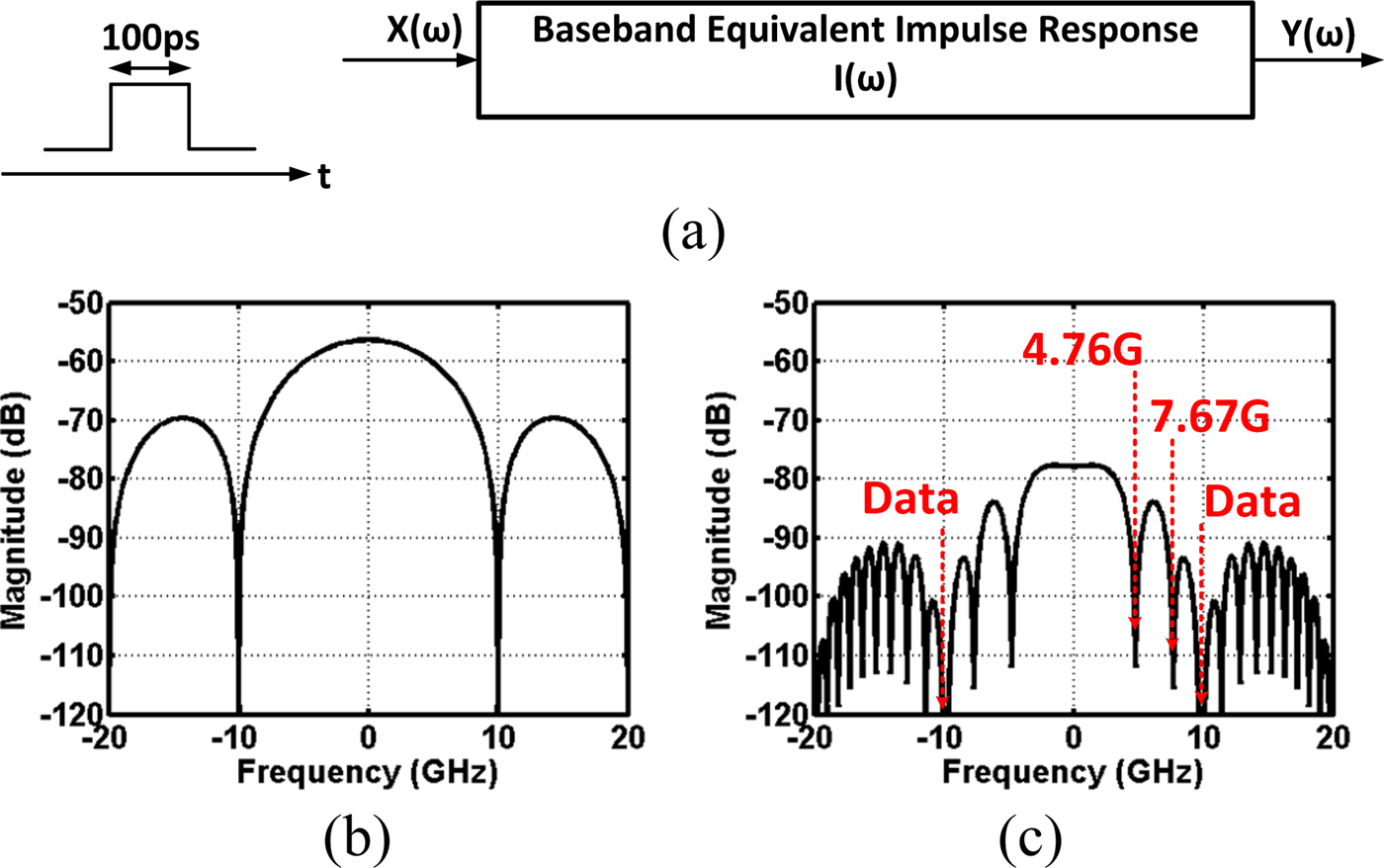
As stated in (3), after having established the impulse response of a waveguide, an output data spectrum can be calculated instantly by multiplying input spectrum and impulse response in frequency domain as shown in Fig. 8. For instance, imagine a 100 ps of single pulse that travels down to a waveguide with a carrier frequency of 100 GHz. In frequency domain, it means a sync function multiplies with an impulse response studied in Fig. 6. Notice that the output spectrum contains notches at 4.76 and 7.67 GHz below 10 GHz (data null). For applications in high-speed data communication through PCB or copper cable, discontinuities such as connectors or via usually create notches in frequency domain by a destructive interference mechanism [Reference Kam and Kim20, Reference Du21]. However, for waveguides under coherent architecture, a non-linear propagation constant, which is a complicated function of waveguide geometry, length, dielectric material, and carrier frequency, generates notches in frequency domain after down-conversion. Fortunately, the proposed analysis could precisely analyze a notch behavior without needing any estimating method.
(a) Impulse response calculation in frequency domain. (b) A 100 ps baseband pulse is generated at the input of waveguide. (c) After taking Fourier transform, input spectrum is fed into the baseband equivalent impulse response of waveguide, and the output spectrum of pulse is generated instantly by multiplying two spectrums. Notice that the notches heavily affect the output spectrum.
C) Time domain impulse response and simulation
In Fig. 9(a), an impulse response of waveguide in time domain is first calculated by taking an inverse Fourier transform of (23) in MATLAB software. Interestingly, a finite delay of modulated wave through a waveguide is also reflected in the baseband impulse response. As suggested in (4), an impulse response in time domain is now convoluted with an input pulse to generate an output pulse. Taking a closer look at Fig. 9(c), when 100 GHz of carrier frequency is used, a 1 m length of dielectric-filled metallic circular waveguide contributes roughly 160 ps of pulse broadening as well as post-cursor and pre-cursor residue. On the other hand, a group delay variation method in (1) and (2) estimates 82 ps of pulse broadening, which is half of what an impulse response method has predicted. To illustrate a group delay variation method briefly, a dispersion coefficient is calculated based on the 10 GHz baseband equivalent bandwidth in Fig. 9(d). The graph shows that a dispersion decreases as carrier frequency increases. In Fig. 9(e), a dispersion from an impulse response is compared with a group delay method with a fixed carrier frequency of 100 GHz for both cases. As expected, a group delay method increases a dispersion coefficient linearly. To be fair, for the case of impulse response, a dispersion is measured while an attenuation constant of waveguide is kept at zero, because a group delay variation method does not consider a dispersion effect from an amplitude response variation at all. At a bandwidth of 10 GHz, the difference between the two increases by 90 ps, which is close to 100% of its original bandwidth. The above analysis verifies how a group delay method is inappropriate for a wideband data communication.
(a) Time domain impulse response is calculated in MATLAB. (b) A 100 ps baseband pulse is generated. (c) Two are convoluted in time domain. A resulting pulse width at the output is increased to 260 ps. (d) Dispersion coefficient with 10 GHz baseband equivalent bandwidth using group delay variation method. (e) Dispersion comparison with group delay and impulse response method.

In order to prove the validity of the frequency domain impulse response expression in (23), a time domain simulation is conducted by stepping through each stage as in Fig. 10(a). An up-converter multiplies input pulse and carrier signal at node B, and the modulated signal undergoes dispersion and distortion at node C. A down-converter translates to a baseband with 2ω 0 residue at node D, and an LPF filters out the 2ω 0 component at node E. As a side note, one can decide to down-convert at node C by way of an envelope detector but with a cost of 400 ps pulse broadening penalty [Reference Kim22]. Comparing Figs 9(c) and 10(e), the two baseband output signals are almost identical except the fact that there is a slight residue of 2ω 0 component left in Fig. 10(e).
(a) Block diagram. (b) Modulated pulse with 100 GHz carrier frequency. (c) Heavily dispersed modulated pulse after going through the waveguide. (d) Down-converted baseband pulse with 2ω 0 residue. (e) Baseband pulse after LPF.

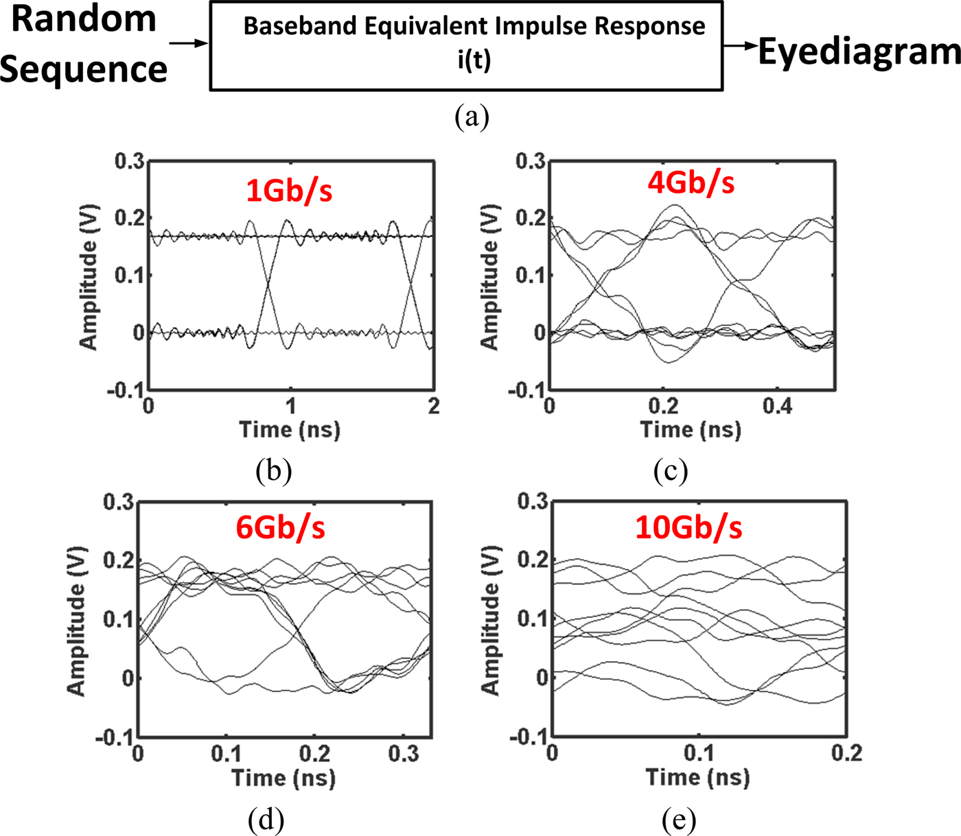
Another crucial advantage of the baseband equivalent impulse response is the ability to simulate a random bit sequence as an input and generate an eye diagram for a given data rate as in Fig. 11. A single pulse informs on a degree of dispersion or distortion, but a measure of inter-symbol interference (ISI) requires a random bit pattern of input. After all, a waveguide transfers lots of digital data consisting of ones and zeros, and by the definition of information conveying signal, they need to be a random combination. Once an impulse response is created, a sequence of randomly combined ones and zeros convolve with an impulse response and produce an eye diagram. For the given waveguide parameters in Fig. 3 and carrier frequency of 100 GHz, it is obvious that 10 Gb/s of data stream is not suitable without any equalization as shown in Fig. 11(e).
(a) Eye-diagram simulation. (b) 1 Gb/s eye diagram. (c) 4 Gb/s eye diagram. (d) 6 Gb/s eye diagram. (e) 10 Gb/s eye diagram.
In summary of sections B and C, the impulse response analysis in frequency domain precisely derives frequency notches that limit waveguide's bandwidth, and additionally, the inverse Fourier transform leads to the time domain impulse response which can study the behavior of wideband baseband signal through waveguides. As discussed in Fig. 9, the discrepancy in dispersion coefficient becomes noticeable as the baseband bandwidth grows larger where narrow band assumption starts falling apart.
D) Effect of phase mismatch
A non-linear propagation constant causes a bandwidth-limiting effect for a high-speed communication system if a phase between transmitter LO and receiver LO is not synchronized. If a propagation constant is a linear function of frequency within a bandwidth of interest, a phase mismatch would reduce a conversion gain but not affect the bandwidth of baseband data. A simple expression can be written based on this assumption,
 $$\eqalign{ y(t) &= x(t)\cos (\omega _0t) \times {\rm cos}(\omega _0t + \theta _M) \cr & = \displaystyle{{x(t)} \over 2}\left[ {\cos (\theta _M) + {\rm cos}(2\omega _0t + \theta _M)} \right],} $$
where θ M is a phase mismatch factor in radian. After filtering out 2ω 0 component, a constant value of cos (θ M) is multiplied to a baseband signal as an indication of reduced conversion gain. However, the situation changes when a propagation constant turns into non-linear. Going back to (23), a new expression with a phase mismatch factor included is written as,
 $$\eqalign{I(\omega ) & = \displaystyle{1 \over 4}F(\omega ) \left[ {e^{ - \alpha (\omega + \omega _0)}e^{ - j\beta (\omega + \omega _0)}e^{ + j ( {\beta ( { - \omega _0} ) + \theta _M} )} }\right. \cr & \qquad \qquad \left. { +\, e^{ - \alpha (\omega - \omega _0)}e^{ + j\beta (\omega - \omega _0)}e^{ - j ( {\beta ( {\omega _0} ) + \theta _M} )}} \right].} $$
It is difficult to grasp what may occur from (26), but an intuitive clue can be deduced from Fig. 7. Earlier, when a phase is synchronized between transmitter and receiver, a notch happens to appear at 4.76 GHz because a receiver LO (100 GHz) and 104.76 + 95.24 GHz signal component is 90° out of phase. It means 104.76 + 95.24 GHz signal is no longer 90° out of phase if a phase of receiver LO moves because of a mismatch. Consequently, as an LO phase shifts, notch frequencies also move, and this behavior repeats every π cycle of θ M. In Fig. 12, the above statement is summarized with a magnitude response of impulse response by solving (26). As a phase mismatch increases up to θ M = (4π/8), the first notch frequency moves towards DC, reducing an effective baseband equivalent bandwidth. At the same time, a magnitude of baseband portion also decreases because of the loss of conversion gain, which is another undesirable side effect. Passing θ M = (4π/8), a notch frequency is pushed out to 6.03 GHz, but now, there is also notch at DC that works as a high-pass filter for a baseband signal. Moving forward, a notch frequency again moves towards DC, but in-band ripple is reduced within 10 dB. An interesting note here is that, with a proper amount of phase mismatch such as in θ M = (7π/8), a baseband signal may take advantage of a free equalization effect with a frequency peaking behavior.
(a) Impulse response when θ M = (2π/8). (b) Impulse response when θ M = (3π/8). (c) Impulse response when θ M = (4π/8). (d) Impulse response when θ M = (5π/8). (e) Impulse response when θ M = (6π/8). (f) Impulse response when θ M = (7π/8).

Concluding this section, the phase mismatch between transmitter and receiver causes additional frequency notches, which emphasizes the importance of carrier synchronization. In addition, it is apparent that phase drift over time will induce extra ISI because of time-varying frequency notches.
E) Effect of carrier frequency
Increasing carrier frequency for a given waveguide improves signal integrity because a wave propagates with TEM-like mode. However, increasing carrier frequency also increases a dielectric loss and the chance of inducing higher order modes. Based on (23), an impulse response in frequency domain at 120 and 150 GHz is plotted in Figs 13(a) and 13(b). With 150 GHz carrier frequency, a notch frequency is pushed out to 10 GHz from 4.76 GHz compared with the 100 GHz case, but loss increases about 3 dB at the same time. In other words, increasing carrier frequency trades a baseband equivalent bandwidth with a signal-to-noise ratio. An apparent improvement of notch frequency can be seen as a carrier frequency increases in Fig. 13(c). For a random sequence testing, an eye opening for 10 Gb/s data stream is clearly visible with 150 GHz carrier frequency, whereas an eye diagram was closed when a carrier frequency is 100 GHz. The impulse response analysis allows us to figure out an exact system requirement once target performance and geometry conditions are known without building actual hardware.
(a) Frequency response with 120 GHz carrier frequency. (b) Frequency response with 150 GHz carrier frequency. (c) Measure of first notch frequency versus carrier frequency. (d) 10 Gb/s eye diagram with 150 GHz carrier frequency.

F) Impact of multimode propagation
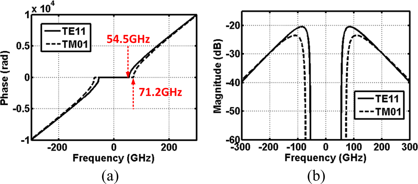
A given waveguide in Fig. 3 supports multiple mode of propagation at 100 GHz, although it may not necessarily excite all possible modes. Even if only one dominant mode is excited at the input, while a wave travels down to a waveguide, a mode conversion may occur because of non-uniform medium or bending curvature. In another case, depending on how a waveguide is excited, a multimode may or may not propagate [Reference Yeh and Shimabukuro23]. It is not the interest of this paper to find out how a multi-mode propagation may occur or how to prevent such an event, but rather figure out how the multimode influences a baseband equivalent impulse response. For brevity, the topic is confined to a two-mode (TE11 and TM01) propagation. To generate a transverse magnetic (TM)-01 mode, relations from (16) to (20) are re-utilized except  $p_{11}^{\prime} $ is replaced by p 01, which is 2.405. As shown in Fig. 14, the second mode begins at 71.2 GHz. According to a field orthogonality theory [Reference Collins24, Reference Imbriale, Otoshi and Yeh25], a transfer function of waveguide and its impulse response can be written as a linear superposition of two transfer functions,
 $$H(\omega ) = C_1H_1(\omega ) + C_2H_2(\omega ),$$
 $$I(\omega ) = C_1I_1(\omega ) + C_2I_2(\omega ),$$
where H 1(ω) and I 1(ω) are dominant modes, H 2(ω) and I 2(ω) are second modes, and C 1 and C 2 are constant coefficients for each mode. An expression for original waveguide frequency response and its impulse response of H 2(ω) and I 2(ω) is configured based on (5) and (23) with α and β updated according to p 01. Caution is required however. In earlier development, a fixed amount of phase is added to a receiver LO to synchronize a phase between transmitter and receiver. The fixed amount of phase was calculated using a dominant mode propagation constant, and the same fixed phase will be employed for both the dominant mode and the second mode, because a dominant mode is always the preferred mode. That is,
 $$\eqalign{I_2(\omega ) & = \displaystyle{1 \over 4}F(\omega ) \left[ {e^{ - \alpha _2(\omega + \omega _0)}e^{ - j\beta _2(\omega + \omega _0)}e^{ + j\beta _1( - \omega _0)} } \right. \cr & \qquad \qquad \left. + e^{ - \alpha _2(\omega - \omega _0)}e^{ + j\beta _2(\omega - \omega _0)}e^{ - j\beta _1(\omega _0) } \right],} $$
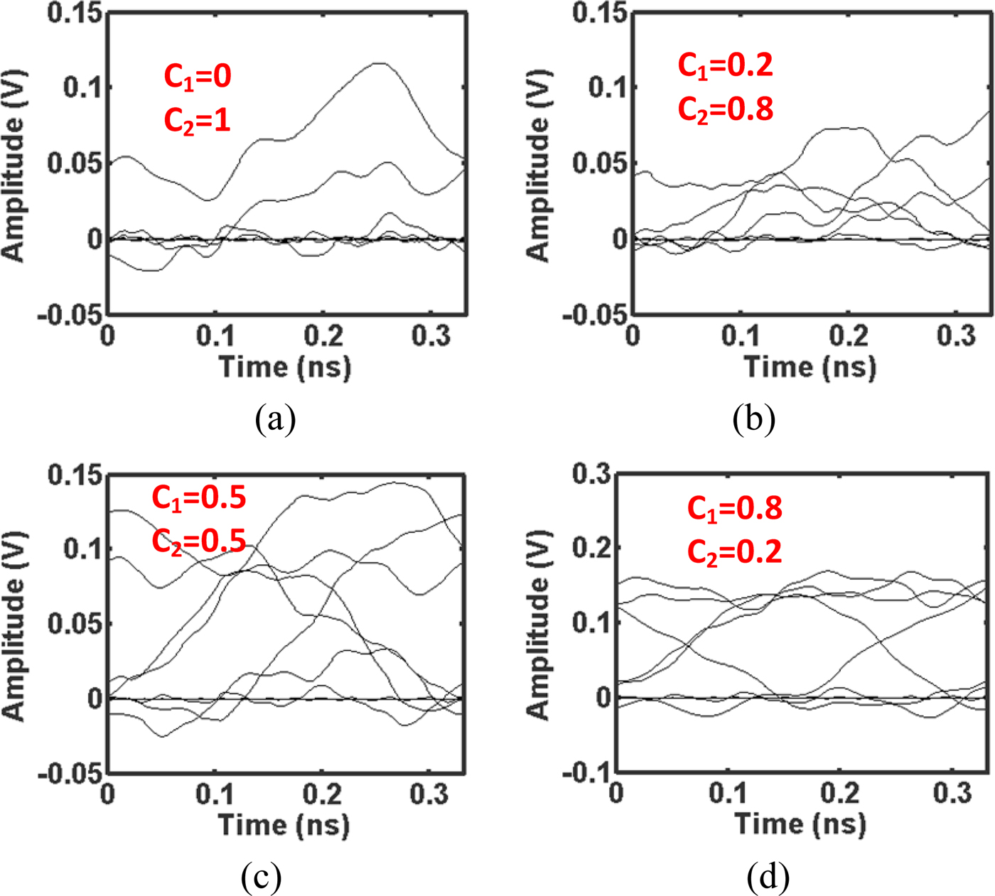
where subscripts 1 and 2 mean dominant mode and second mode. When C 2 = 0, only a dominant mode propagates, and when C 1 = 0, only a second mode propagates. When both are non-zero, both modes would propagate, but again, calculating each coefficient itself under certain circumstance is not the interest. It is assumed that the coefficients are given (for instance, C 1 = 0.8 and C 2 = 0.2), and they are inserted into (28) to see how impulse response responds. With a given waveguide geometry and carrier frequency, it is obvious to anticipate a multimode propagation increases a multi-path effect and corrupts a signal integrity. A few combinations of coefficients are chosen and corresponding impulse responses in frequency domain are plotted in Fig. 15. As described in Fig. 15(a), when only a second mode propagates, the first notch in impulse response shows up at 1.7 GHz compared with 4.76 GHz in a dominant mode case, an interpretation of less baseband equivalent bandwidth. Once they propagate together, an impulse response fluctuates even at very low frequency as in Figs 15(b) and 15(c). However, after a certain threshold ratio of coefficients, an impulse response restores closer back to its original dominant mode response in Fig. 15(d). To glimpse how badly it influences a signal integrity, an eye-diagram test is performed at a fixed data rate of 6 Gb/s. In Figs 16(a) and 16(b), an eye diagram is almost completely closed, and it starts to open in Fig. 16(c) with 0.5 of coefficient for each mode. As proven in this study, a multimode propagation is highly undesirable for a high-speed data communication. To suppress a higher order mode propagation, one can reduce a radius of waveguide at a target carrier frequency, but it will reduce a bandwidth capacity by pulling a notch frequency towards DC. By all means, however, it is better to suppress a multimode propagation; if not, at least the amount of presence should be limited as suggested in Figs 15(d) and 16(d).
(a) Phase response of TE11 and TM01 modes. (b) Magnitude response of TE11 and TM01 modes.
Carrier frequency is 100 GHz. (a) Frequency response with C 1 = 0 and C 2 = 1. (b) Frequency response with C 1 = 0.2 and C 2 = 0.8. (c) Frequency response with C 1 = 0.5 and C 2 = 0.5. (d) Frequency response with C 1 = 0.8 and C 2 = 0.2.

Carrier frequency is 100 GHz and the data rate is 6 Gb/s. (a) Eye diagram with C 1 = 0 and C 2 = 1. (b) Eye diagram with C 1 = 0.2 and C 2 = 0.8. (c) Eye diagram with C 1 = 0.5 and C 2 = 0.5. (d) Eye diagram with C 1 = 0.8 and C 2 = 0.2.
IV. AIR-FILLED METAL RECTANGULAR WAVEGUIDE
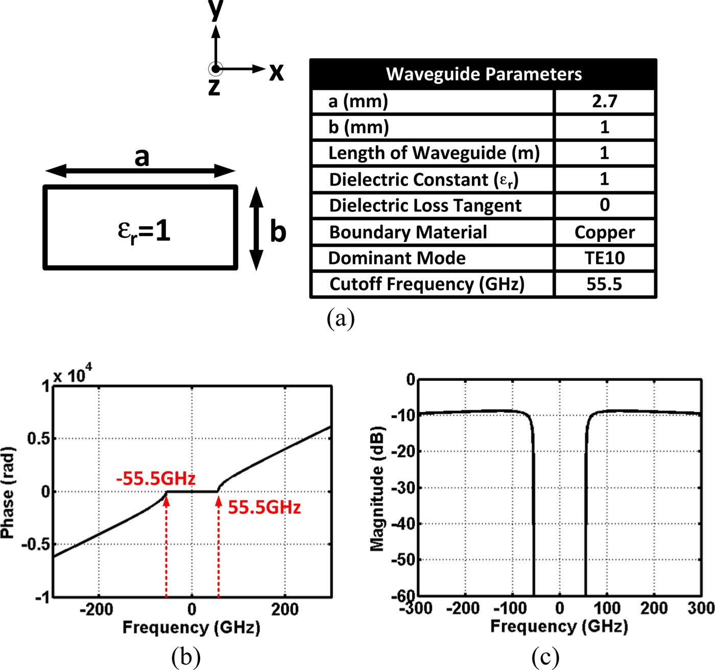
An example of air-filled metal rectangular waveguide is presented in this section to demonstrate how easily a concept of impulse response applies to other types of waveguide. Just as a circular waveguide case, a rectangular waveguide parameter is summarized in Fig. 17 along with a phase and magnitude response. A dimension is decided to place a cutoff frequency at 55.5 GHz, which is close to the circular waveguide case (54.5 GHz). This time, a dielectric material is removed inside, so a loss factor primarily depends on a conductive loss. To summarize a waveguide property,
 $$Cutoff\,wavenumber:k_{c10} = \displaystyle{\pi \over a},$$
 $$Propagation\,constant:\beta _{10} = \sqrt {k^2 - k_{c10}^2}, $$
 $$\eqalign{& Conductive\,Atten.\, constant:\sigma _c \cr & \qquad = \displaystyle{{R_S} \over {a^3bk\eta \beta}} \left( {2b\pi ^2 + a^3\pi ^3} \right)},$$
 $$Cutoff\,{\rm} frequency:\omega _{c10} = \displaystyle{1 \over {a\sqrt {\mu \epsilon}}}. $$
(a) Cross-section of air-filled metallic rectangular waveguide is shown with its propagation parameters. Wave propagates along the z-direction. (b) Phase response. (c) Magnitude response.
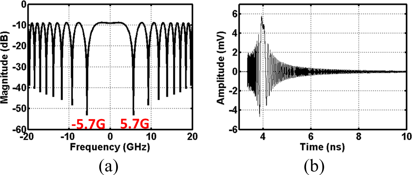
Using relationships of (23), and (30) to (33) with a carrier frequency of 100 GHz, a baseband equivalent impulse response both in frequency domain and time domain is plotted in Fig. 18. A similar time domain simulation is performed as in Fig. 10, but in order to give a different perspective, each time domain signal is represented in frequency domain spectrum in Fig. 19. A single pulse with 100 ps width signal is up-converted using a 100 GHz carrier at node B, and it goes through a waveguide at node C. Notice the effect of cutoff to the modulated spectrum. After down-conversion, it generates both baseband and 2ω 0 spectral components, and an LPF extracts a baseband only at node D.
(a) Baseband equivalent impulse response in frequency domain. (b) Baseband equivalent impulse response in time domain.
(a) Block diagram. (b) Frequency domain-modulated 100 ps pulse with 100 GHz carrier frequency. (c) Frequency domain-modulated pulse after going through the waveguide. (d) Frequency domain down-converted baseband pulse with 2ω 0 residue. (e) Frequency domain baseband pulse after LPF.

V. CONCLUSION
An impulse response method is introduced to analyze the information capacity of waveguides for high-speed data communication applications. Traditional group delay variation methods can only predict pulse broadening effect when transmitted data bandwidth is narrow. Consequently, it does not fully reveal non-linear ISI effect corresponding to random baseband data sequences.
Instead, our newly proposed approach is able to capture complete non-linear behavior of baseband equivalent signal propagation under coherent communication system for any given waveguide geometry and carrier frequency, and produce impulse responses in both time and frequency domains.
Eye diagrams are also finally constructed based on time domain impulse response for a random baseband bit sequence input, which is the most essential performance metric for quantifying data communication speed and bit error rate.
 Yanghyo Kim completed his Ph.D. at the University of California, Los Angeles in 2017. While he was working for Keyssa Inc. from 2010 to 2013, he commercialized the first 60 GHz CMOS contactless connector system. He is now with the Jet Propulsion Laboratory as a postdoctoral fellow, developing CMOS system-on-chip (radar, radiometer, spectrometer) for space applications.
 Adrian Tang is a senior member of the IEEE and has over 15 years of CMOS/SiGe IC design experience in both research and commercial wireless environments with projects ranging from commercial Bluetooth and WLAN chipsets to mm-wave and THz chipsets for communication, radar, and spectrometer systems. Since joining JPL in 2013, Adrian was the first to demonstrate sub-centimeter accurate mm-wave imaging radar in silicon technology with demonstrations at 144 and 155 GHz, the first to demonstrate pre-distortion in CMOS mm-wave transmitters above 150 GHz, and the first to demonstrate CMOS-based passive radiometers with enough sensitivity to support passive imaging. At JPL, Adrian is currently leading development of a wide range of CMOS SoC chipsets for planetary, Earth science, and astrophysics space instruments. Since joining in 2013 Adrian has designed and fabricated over 165 successful CMOS chips at JPL, including 46 full SoCs.
 Jason Cong received his B.S. degree in Computer Science from Peking University in 1985, his M.S. and Ph. D. degrees in Computer Science from the University of Illinois at Urbana-Champaign in 1987 and 1990, respectively. Currently, he is a Chancellor's Professor at the Computer Science Department, also with joint appointment from the Electrical Engineering Department, of the University of California, Los Angeles, the director of Center for Domain-Specific Computing (CDSC), and the director of VLSI Architecture, Synthesis, and Technology (VAST) Laboratory. He served as the Chair at the UCLA Computer Science Department from 2005 to 2008, and is also a distinguished visiting professor at Peking University. Dr. Cong's research interests include synthesis of VLSI circuits and systems, programmable systems, novel computer architectures, nano-systems, and highly scalable algorithms. He has over 400 publications in these areas, including 10 best paper awards, two 10-Year Most Influential Paper Awards. He was elected to an IEEE Fellow in 2000 and ACM Fellow in 2008, and received two IEEE Technical Achievement Awards, one from the Circuits and System Society (2010) and the other from the Computer Society (2016).
 Mau-Chung Frank Chang is currently the President of National Chiao Tung University, Hsinchu, Taiwan. He is also the Wintek Chair Professor of Electrical Engineering with the University of California, Los Angeles, CA, USA. His research interests include the development of high-speed semiconductor devices and high-frequency integrated circuits for radio, radar, and imaging system-on-chip applications up to terahertz frequency regime. Dr. Chang is a member of the US National Academy of Engineering, a fellow of the US National Academy of Inventors, and an Academician of Academia Sinica of Taiwan. He was honored with the IEEE David Sarnoff Award in 2006 for developing and commercializing GaAs HBT and BiFET power amplifiers for modern high-efficiency and high-linearity smart phones throughout the past 2.5 decades.
 Tatsuo Itoh received the Ph.D. degree in Electrical Engineering from the University of Illinois at Urbana–Champaign, Champaign, IL, USA, in 1969. He was with the University of Illinois at Urbana–Champaign, SRI, and the University of Kentucky, Lexington, KY, USA. In 1978, he joined the University of Texas at Austin, Austin, TX, USA, where he was a Professor of electrical engineering in 1981 and a Hayden Head Centennial Professor of Engineering in 1983. In 1991, he joined the University of California at Los Angeles, Los Angeles, CA, USA, as a Professor of electrical engineering and the TRW Endowed Chair of Microwave and Millimeter Wave Electronics (currently the Northrop Grumman Endowed Chair). He has authored over 440 journal publications, 880 refereed conference presentations, and 48 books/book chapters in the area of microwaves, millimeter waves, antennas, and numerical electromagnetics. He has generated 80 Ph.D. students. Dr. Itoh is a member of the Institute of Electronics and Communication Engineers of Japan and the Commissions B and D of USNC/URSI. He was a recipient of the IEEE Third Millennium Medal in 2000, the IEEE MTT-S Distinguished Educator Award in 2000, the Outstanding Career Award from the European Microwave Association in 2009, the Microwave Career Award from the IEEE MTT-S in 2011, and the Alumni Award for Distinguished Service from the College of Engineering, University of Illinois at Urbana–Champaign in 2012. He was an elected member of the National Academy of Engineering in 2003. He served as the Editor of the IEEE TRANSACTIONS ON MICROWAVE THEORY AND TECHNIQUES from 1983 to 1985. He was the President of the IEEE MTT-S in 1990. He was the Editor-in-Chief of IEEE MICROWAVE AND GUIDED WAVE LETTERS from 1991 to 1994. He was elected as an Honorary Life Member of the MTT-S in 1994. He was the Chairman of Commission D of International URSI from 1993 to 1996. He served as a Distinguished Microwave Lecturer on Microwave Applications of Metamaterial Structures of the IEEE MTT-S from 2004 to 2006. He serves on the advisory boards and committees of a number of organizations.



