





Introduction
Riverine ecosystems are increasingly threatened by water pollution, diversion, damming, sand mining, and other anthropogenic activities (Sabater et al. Reference Sabater, Bregoli, Acuña, Barceló, Elosegi, Ginebreda, Marcé, Muñoz, Sabater-Liesa and Ferreira2018). Global biological assessments indicate that up to 50% of rivers across various countries have degraded over time (Feio et al. Reference Feio, Hughes, Callisto, Nichols, Odume, Quintella, Kuemmerlen, Aguiar, Almeida, Alonso-EguiaLis, Arimoro, Dyer, Harding, Jang, Kaufmann, Lee, Li, Macedo, Mendes, Mercado-Silva, Monk, Nakamura, Ndiritu, Ogden, Peat, Reynoldson, Rios-Touma, Segurado and Yates2021). In population-dense countries, additional stressors such as encroachment and human alteration of riverbanks alter the riparian flora and fauna over time. In India, riparian protection rules or policies are largely absent outside protected areas. As a result, riparian areas are highly vulnerable. They continue to degrade and require interventions at landscape or regional scales. Although India has a monitoring infrastructure in place to periodically analyse water quality parameters, flow, and discharge (India WRIS n.d.), such data are primarily helpful for water resources and dam management and river use classification (Singh and Saxena Reference Singh and Saxena2018). But these are insufficient to determine the comprehensive health profile of the rivers.
People and managers often see rivers as channels carrying water, rarely recognizing the zone beyond the channel—the terrestrial-aquatic continuum. Also known as riparian zones, these are unique zones of transition between land and water (Junk et al. Reference Junk, Bayley and Sparks1989). Riparian zones interact with the surface water, sub-surface water, and the land, shaping the riverine ecosystem (Thorp et al. Reference Thorp, Thoms and Delong2008; Ward Reference Ward1998). The continuum is characterized by specialized flora and fauna that perform unique ecosystem functions such as nutrient cycling (fishes, turtles), erosion prevention (vegetation), and seed dispersal (birds, animals). The status of riparian vegetation or riparian zones has been widely used as a proxy for river health and ecological integrity (Fernández et al. Reference Fernández, Barquín, Álvarez-Cabria and Penas2014; Macfarlane et al. Reference Macfarlane, Gilbert, Jensen, Gilbert, Hough-Snee, McHugh, Wheaton and Bennett2017; Michez et al. Reference Michez, Piégay, Lisein, Claessens and Lejeune2016; Vidal-Abarca et al. Reference Vidal-Abarca, Santos-Martín, Martín-López, Sánchez-Montoya and Alonso2016; Werren and Arthington Reference Werren and Arthington2002).
The concept of river health includes both ecological and human (social) components and emphasizes biotic assessment alongside physico-chemical parameters (Boulton Reference Boulton1999; Norris and Thoms Reference Norris and Thoms1999; Wang et al. Reference Wang, Zhang, Yang, Zhang, Li and Chen2019). Most river health assessment frameworks consider physical habitat, hydrology, biology, water quality, and geomorphology. This is similar to some of the earliest diagnostic tools, e.g., one discussed by Maddock (Reference Maddock1999). These attributes are often consolidated into indices, such as the Index of Biotic Integrity (IBI) developed by Karr (Reference Karr1999), who also attempted to define river health. IBI was developed in USA and involves twelve metrics based on species richness and abundance of functional groups of fishes (Karr et al. Reference Karr, Fausch, Angermeier, Yant and Scholosser1986). Since Karr’s work, both the biological and integrated (physical, chemical, and biological) multi-metric indices have been tested and utilized for river health assessment (Cupertino et al. Reference Cupertino, Dufour and Rodríguez-González2024; Kim and An Reference Kim and An2015; Shi et al. Reference Shi, Liu, You, Bao, Meng and Chen2017; Zhang et al. Reference Zhang, Meng, Xia, Wu and She2018). These indices continue to appeal non-expert users and decision-makers because they can simplify the complex and large datasets.
Depending on the assessment and monitoring goals, biological indices employ either a representative biotic community (e.g., fishes) or sentinel species, also known as ‘Ecosystem Sentinels’ (Hazen et al. Reference Hazen, Savoca, Clark-Wolf, Czapanskiy, Rabinowitz and Abrahms2024). Communities such as riparian vegetation (Aguiar and Ferreira Reference Aguiar and Ferreira2005; Malik et al. Reference Malik, Shinwari and Waheed2012; Pinto and Araújo Reference Pinto and Araújo2007; Roth et al. Reference Roth, Allan and Erickson1996), micro-and macro-invertebrates (Burdon et al. Reference Burdon, Ramberg, Sargac, Forio, De Saeyer, Mutinova, Moe, Pavelescu, Dinu, Cazacu, Witing, Kupilas, Grandin, Volk, Rîşnoveanu, Goethals, Friberg, Johnson and McKie2020), insects (Vieira et al. Reference Vieira, Dias-Silva and Pacífico2015; Viegas et al. Reference Viegas, Stenert, Schulz and Maltchik2014), and fishes (Pinto and Araújo Reference Pinto and Araújo2007; Snyder et al. Reference Snyder, Young, Villella and Lemarie2003; Vieira et al. Reference Vieira, Dias-Silva and Pacífico2015) are more widely employed in computing indices of riparian health because of their sensitivity to disturbance and well-established methodology for assessment. The choice of species (or community) also depends on the response of the species to the stressors, species abundance, distribution, and ease of monitoring. For example, Jia and Chen (Reference Jia and Chen2013) used two fish species, Xenocypris davidi and Hemibarbus labeo, as sentinel species for the Dongjiang River in China, and Grove et al. (Reference Grove, Henny and Kaiser2009) used Osprey Pandion haliaetus for aquatic ecosystems in the United States. Bats are also potential bioindicators but have limited research and show mixed outcomes for assessing river water quality or health (de Conno et al. Reference de Conno, Nardone, Ancillotto, De Bonis, Guida, Jorge, Scarpa and Russo2018; López-Bosch et al. Reference López-Bosch, Blanch, Páramo, Flaquer-Sánchez and López-Baucells2024; Russo et al. Reference Russo, Salinas-Ramos, Cistrone, Smeraldo, Bosso and Ancillotto2021). Similarly, amphibians have been used to compute IBI for wetlands in the USA (Micacchion Reference Micacchion2002; Shulse et al. Reference Shulse, Semlitsch and Trauth2009, Welsh and Hodgson Reference Welsh2008), due to their sensitivity to multiple stressors, including changing water quality (Calderon et al. Reference Calderon, Almeida, González and Jofré2019).
The IBI remains a popular biological index and was later modified by several authors (Pérez-Domínguez et al. Reference Pérez-Domínguez, Maci, Courrat, Lepage, Borja, Uriarte, Neto, Cabral, Raykov, Franco and Alvarez2012). IBI mainly uses fishes and is particularly popular in the USA (Capmourteres et al. Reference Capmourteres, Rooney and Anand2018; Fausch et al. Reference Fausch, Karr and Yant1984), Europe (Breine et al. Reference Breine, Van den Bergh, Van Thyune and Belpaire2021; Oberdorff and Hughes Reference Oberdorff and Hughes1992; Oberdorff and Porcher Reference Oberdorff and Porcher1994,) and New Zealand (Joy and Death Reference Joy and Death2004; Joy et al. Reference Joy, Foote, McNie and Piria2018), but sparsely used in South Asian countries (Gonino et al. Reference Gonino, Benedito, Cionek, Ferreira and Oliveira2020). There are several multi-metric fish-based indices other than IBI, differing in number and nature of metrics and method of aggregation, and are mostly tested in the USA, Europe, and Africa (Pérez-Domínguez et al. Reference Pérez-Domínguez, Maci, Courrat, Lepage, Borja, Uriarte, Neto, Cabral, Raykov, Franco and Alvarez2012). In Indian streams, phytoplanktons (Kamboj et al. Reference Kamboj, Kamboj, Sharma and Bisht2022), benthic macro-invertebrates (Harikumar et al. Reference Harikumar, Deepak and Ramachandran2014; Sharma and Rawat Reference Sharma and Rawat2009; Singh et al. Reference Singh, Sharma, Sharma and Mishra2019), diatoms (Srivastava et al. Reference Srivastava, Grover, Verma and Khan2017), insects (Chakravarty and Gupta Reference Chakravarty and Gupta2024), and fishes (Bhat Reference Bhat2017; Das and Samanta Reference Das and Samanta2006; Ganasan and Hughes Reference Ganasan and Hughes1998; Sajina et al. Reference Sajina, Sudheesan, Samanta, Paul, Bhowmick, Nag, Kumar and Das2022) have been used to assess river health but a multi-index approach has not been tested so far. Among the existing biotic indices, only the IBI (Karr Reference Karr1981) has been tested in Central (Ganasan and Hughes Reference Ganasan and Hughes1998), Northern (Das and Samanta Reference Das and Samanta2006), and Peninsular India (Bhat Reference Bhat2017; Nair et al. Reference Nair, Muhammadali, Koushlesh, Chanu, Das, Bhakta, Pillai, Gogoi, Samanta, Meetei, Baitha, Kamble, Kumar and Das2023; Sajina et al. Reference Sajina, Sudheesan, Samanta, Paul, Bhowmick, Nag, Kumar and Das2022), although the individual metrics used in these studies vary.
Birds are also an important taxon for river health assessment but their use in indices has been limited (Bryce et al. Reference Bryce, Hughes and Kaufmann2002; Larsen et al. Reference Larsen, Sorace and Mancini2010; Young et al. Reference Young, Ammon, Weisberg, Dilts, Newton, Wong-Kone and Heki2013). Bird Integrity Index (BII) was developed in the United States to assess utility of bird assemblages to inform riparian condition (Bryce et al. Reference Bryce, Hughes and Kaufmann2002). This was based on data from 13 sites (one km long reaches) along wadable streams of Willamette Valley of Oregon state. They tested metrics that would respond to disturbance irrespective of the theoretical and conceptual explanations.
Besides the biological indices, several indices assess the physical habitat in riparian areas. Peterson (Reference Petersen1992) developed the Riparian, Channel, Environmental Inventory involving 16 attributes that focus on stream channel and riparian zone morphology, and habitat conditions of small streams. Building on this rationale, Qualitat del Bosc de Ribera (QBR) was developed in Spain but focuses on zones beyond permanently flowing water and up to the bank-full width (Munné et al. Reference Munné, Prat, Solà, Bonada and Rieradevall2003). Similar to QBR and also developed in Spain is the Riparian Quality Index, which brings additional information on longitudinal continuity, natural regeneration, and lateral and vertical connectivity (González del Tánago and García de Jalón Reference González del Tánago and García de Jalón2011). Other commonly used measures for riparian habitat assessment are the qualitative habitat evaluation index and the rapid bioassessment protocols. In further assessments, these have been correlated with biological indices such as IBI (Stauffer and Goldstein Reference Stauffer and Goldstein1997).
Recently, the availability of high spatial resolution satellite images has been easing the calculation of Riparian Strip Quality Index (RSQI). It was originally formulated by Saint-Jacques and Richard (Reference Saint-Jacques and Richard1998) using aerial images for Chaudière River in Québec, Canada. It essentially quantified the quality of riparian strip as a sum of proportion of different land uses, weighted by their ability to maintain certain ecological functions. The weights are based on eleven ecological functions on which each land use was scored depending on their ability to provide these functions (Saint-Jacques and Richard Reference Saint-Jacques and Richard1998). Some authors have tested this index in India (Nag et al. Reference Nag, Sharma, Rallapalli, Puppala, Kumar, Lenhart and Goonetilleke2026; Saha et al. Reference Saha, Das, Dasgupta and Patel2020), Spain (Rivas-Fandiño et al. Reference Rivas-Fandiño, Acuña-Alonso, Novo, Pacheco and Álvarez2023), and South Korea (Machado and Kim Reference Machado and Kim2024). It requires land use and land cover (LULC) maps which have been derived from very high-resolution (1.85 m) images from Worldview-2 satellite (Rivas-Fandiño et al. Reference Rivas-Fandiño, Acuña-Alonso, Novo, Pacheco and Álvarez2023) to high-resolution (10 m and 20 m) images of Sentinel-2 MSI (Machado and Kim Reference Machado and Kim2024). An extension of this index, Riparian Strip Efficiency Index, was proposed to include hydrological and topographical variables (Novoa et al. Reference Novoa, Chokmani and Lhissou2018). It was designed for Canada and Nordic countries where there is concentrated and rapid runoff from snow-melt and spring rains.
One of the limitations of the biological indices is their focus on one taxon, which limits the riparian assessment to one component, i.e., either the aquatic or the terrestrial. Gurjar et al. (Reference Gurjar, Lakhera, Vyas and Raina2023) suggested the use of an Integrated River Health Assessment System involving the Water Quality Index, Stream Water Index, Index of Biotic Integrity, Physical Habitat Index, Qualitat del Bosc de Ribera (QBR), Biological Monitoring Working Party, Average Score Per Taxon, and Hilsenhoff Biotic Index, but it remains a suggestion. A recent initiative (2020–2025) undertaken by the Government of India called the Long-Term Ecological Observatories (LTEO) programme monitors multi-taxa populations across six landscapes in India involving multiple institutions (https://lteo.iisc.ac.in/). Fishes are one of the taxa being studied using IBI in four Indian landscapes (north, east, central, and the south). A holistic assessment tool or index that can be economically incorporated into regular monitoring will be useful in this context since there is a lack of established monitoring frameworks and funding mechanisms, both at the regional and national level.
In this study, we test three biological indices involving fishes, birds, and plants and one LULC based index, representing the land, water, and the transition zone. We complement this information with stream physico-chemical characteristics, for a comprehensive assessment of river health. The indices are the IBI (Karr Reference Karr1981), Biotic Integrity Index (BII) (Bryce et al. Reference Bryce, Hughes and Kaufmann2002), QBR (Munné et al. Reference Munné, Prat, Solà, Bonada and Rieradevall2003), and RSQI (Saint-Jacques and Richard Reference Saint-Jacques and Richard1998). Our objectives were (i) to test and adapt these indices to the streams in southern India and (ii) to assess their ability to distinguish between segments of different health status, while focussing on the terrestrial-aquatic continuum.
Materials and methods
Study area
We conducted this study in the Cauvery Watershed in southern India (Figure 1). The riparian areas lie largely within a forest-agriculture matrix. The Cauvery River drains the ‘rice bowl’ of India covering an area of 81,155 sq. km, into the Bay of Bengal. In the upstream region, it flows through forested areas but soon transitions into an agriculture-intensive region. We focused on the Moyar-Bhavani-Noyyil sub-watershed (area = 28012.79 sq. km), one of the nine sub-watersheds of the Cauvery, but did not consider Noyyil river. Moyar is considered one of the intact rivers in the Cauvery watershed, allowing a meaningful comparison with degraded sites.
Study area and the sampled sites (segments). Subset (a) India with state boundaries showing study region in southern India, (b) location of the Moyar-Bhavani-Noyyil sub-watershed (shown with blue background) within the cauvery watershed; (c) sampling points. Data source: drainage network–Hydrosheds HydroRivers v1.0 (Lehner and Grill Reference Lehner and Grill2013; Forest Cover–Forest Survey of India 2015); Dams, barrage, weirs, anicut, powerhouses– Open Government Data Platform India; Protected areas of India– Wildlife Institute of India.

Figure 1. Long description
Panel A: A map of India highlighting the study region in southern India with state boundaries. The study region is marked with a red box. Panel B: A detailed map showing the location of the Moyar-Bhavani-Noyyil sub-watershed within the Cauvery watershed, highlighted with a blue background. The drainage network is depicted with varying line thicknesses indicating different drainage orders. Panel C: A zoomed-in map of the study area showing specific sampling points. The map includes various symbols indicating pilot survey points, surveyed points, reconnaissance points, dams, barrages/weirs/anicuts, and powerhouses. The drainage network is shown with different line thicknesses representing different drainage orders. Protected areas and forest cover are also indicated with different shading patterns. Key rivers such as the Moyar River, Bhavani River, and Cauvery River are labeled. The sampled sites are numbered and labeled with their respective names.
The Moyar River is 90 km long, originating in the Nilgiri district of Tamil Nadu state in the Western Ghats (a biodiversity hotspot) and joining the Bhavani River at Bhavanisagar Dam in Erode district of Tamil Nadu state. The Bhavani River is 215 km long and meets the Cauvery River downstream of this dam. The mean elevation of the Moyar-Bhavani sub-watershed is 815.6 m, and the mean slope is 10.2 degrees. Temperature in the Bhavani River watershed ranges between 29.6°C and 19°C (Kamalamma et al. Reference Kamalamma, Babel, Sridhar and Vellingiri2023), and it gets an average rainfall of 811.5 mm (544.7 mm–2251.0 mm) (CGWB 2017). The average discharge at Thengumarhda (Moyar River) has been recorded as 375.2 m3 s−1, ranging between 360.5 m3 s−1 and 535.1 m3 s−1 for the period 01 Jan 2020–07 Sep 2025 (Patidar et al. Reference Patidar, Indu and Karmakar2024). Average discharge at Nellithurai (Bhavani River) has been recorded as 134.6 m3 s−1, ranging between 2.7 and 768.9 m3 s−1 for the period 01 Jan 2020–28 July 2025 (Patidar et al. Reference Patidar, Indu and Karmakar2024). Dominant forest types in this region are mixed dry deciduous and thorn forests, with some patches of moist teak forests and scrub (Table S1). The agricultural lands have both monocultures and mixed plantations of coconut, areca nut, banana, and crops like mustard and paddy with interspersed grazing lands.
Sampling approach
We followed a nested hierarchical sampling framework (Frissell et al. Reference Frissell, Liss, Wissmar and Hurley1986) for river segment selection. This framework is useful for complex, multi-scale ecological studies, especially in riverine ecosystems, and has been utilized for fish assemblage assessments (Atkore Reference Atkore2017; Boys and Thoms Reference Boys and Thoms2006; Perez Rocha et al. Reference Perez Rocha, Cottenie, Clein, Elkins, Mangold, Nowlin, Perkin, Wright and Schwalb2024). Within the Moyar-Bhavani-Noyyil sub-watershed, we selected segments and reaches based on the stream order, land use type, and bed and bank characteristics. We chose segments of one-km length to accommodate bird and disturbance sampling (Bryce Reference Bryce2006). Within any one-km segment, we found variations in substrate (sand bars or rocky islands), vegetation (shrub dominant or tree dominant), and disturbance. Therefore, smaller reaches of 100 m–200 m length were not representative of the local variations in habitat type. Additionally, Saint-Jacques and Richard (Reference Saint-Jacques and Richard1998) opine that given the mobility of fishes, segments of approximately two km are sufficient to detect the effect of habitat degradation on fishes. Potential segments were identified using forest cover maps, Google Earth (for road networks), and knowledge from recent studies in the region (Atkore et al. Reference Atkore, Kavin, Choudhary and Johnson2023). Both QBR and BII required walkable banks. In a pilot sampling session conducted in May 2022, we determined the sampling protocol to suit the study site and determined the accessibility (walkability, maximum length walkable), stream wadability, and similarity among the riparian habitats. Because this study was designed to test the overall approach, we limited our sampling from 18 potential segments to nine sampled segments (44 reaches) (Figure 1).
Sampling methods
We conducted surveys for biotic communities and habitat characteristics, surveying 44 reaches/plots along nine segments between May and July 2022. We walked along the riverbank and used the point count method to record birds every 250 m (Bibby Reference Bibby, Jones and Marsden1998; Bryce et al. Reference Bryce, Hughes and Kaufmann2002) (Figure 2). Birds sighted within a 10 m radius were recorded, and the observation period at each point lasted 10 minutes. At the same points, we sampled vegetation in 10 m × 10 m plots for trees, 5 m × 5 m for shrubs, and 1 m × 1 m for herbs, grasses, sedges, and saplings (Table S2). We categorized vegetation into trees, shrubs, herbs, grasses/sedges, ferns, saplings, creepers, and climbers and noted any invasive species separately. For fishes, we chose a 150 m long reach with a pool-run-rapid character within the one-km segment. We used the catch-and-release method to sample fishes and employed local methods involving cast nets (∼2 cm × 2 cm), gill nets (2.5 cm × 2.5 cm), and drag nets (0.1 × 0.1) (Table S3) following Atkore et al. (Reference Atkore, Kavin, Choudhary and Johnson2023) and Bhat (Reference Bhat2017). For all the sites and replicates, fishing gear remained same (cast and drag nets), except for two sites, where using cast nets was not possible. Gill nets are difficult to use in streams with high discharge or low depth. Gill nets were used in two higher depth segments (Kargudi and Theppekadu) after the cast nets failed to capture fishes. While using three types of nets, we ensured that total sampling time was similar for all sites and replicates, i.e., approximately 1.5–2 hours. For each effort, we measured and photographed the fishes and released them alive into the river. We used abundance data of fishes and birds for extrapolation and rarefaction to understand sample coverage using the iNEXT package in R (Chao et al. Reference Chao, Gotelli, Hsieh, Sander, Ma, Colwell and Ellison2014; Hsieh et al. Reference Hsieh, Ma and Chao2024; R Core Team 2023) setting at 50 bootstraps and a 0.95 level of confidence.
Sampling design showing a segment and the five plots/reaches sampled. Figure created in Canva.

We measured water quality, water depth (m), river width (m), and stream velocity (m s−1) at the site of fish sampling and estimated stream discharge (m3 s−1) using the measured variables. To measure water quality, we used a multi-parameter water quality metre—HI98194 (Hanna Pvt. Ltd.) and recorded five physico-chemical variables (Table S2). We computed stream velocity (m s−1) using river cross-section (measured manually) and velocity (measured using a flowmeter—Geopacks Advanced stream flow metre, UK) (Figure S1). We supplemented this information with riverbed and bank characteristics recorded every 250 m by visual observation (Table S2, Figure 2). We only considered disturbance indicators that could be observed at the stream or riparian scale, for example, human habitation, noise, fishing, etc. We recorded disturbance at the sites of bird counts, i.e., every 250 m along the trail, and pooled the information for the segment-scale analysis (Figure 2, Table S4).
Computing indices
IBI
Most studies computing IBI have used 11–12 metrics, but these differ to suit the study site and fish population (Table S5). We followed methods described in Ganasan and Hughes (Reference Ganasan and Hughes1998) and adapted the metrics. We omitted the fish health metric, because it required capture and detailed assessment. Further, our categorization of native species was in context of the Western Ghats region which led to many fish families having both native and non-native species. Therefore, we omitted the ‘number of native fish families’ metric. We instead considered both ‘total non-native species’ and ‘total non-native individuals’ as presence of non-native individuals presents a concerning shift in fish community composition and can indicate anthropogenic changes in the landscape (Joshi et al. Reference Joshi, Alam, Jha, Srivastava and Kumar2016; Kharat et al. Reference Kharat, Dahanukar, Raut and Mahabaleshwarkar2003; Sreekanth et al. Reference Sreekanth, Mujawar, Lal, Mayekar, Stephen, Raghavan, Kumar and Ingole2022). We calculated ten metrics in total (Table S5). We classified fish species based on feeding depth, feeding guild, and tolerance, using available literature, involving both peer-reviewed sources and online databases. We categorized fish species as intolerant, if they had a narrow preference range of food, water depth and water temperature. We then scored the metrics using the trisection method (Ganasan and Hughes Reference Ganasan and Hughes1998; Karr Reference Karr1981), assigning a score of 1, 3, or 5 for each of the ten metrics. Here, a higher score reflects higher integrity (or less degradation). Finally, we added the scores of ten metrics to get the IBI values for each segment.
Disturbance index
We recorded different sources of disturbance observed during field sampling and recorded their presence/absence, number, or intensity, as appropriate, at the reach scale. We consolidated them as 15 variables, which were scored either at ratio scale (for quantitative variables) or ordinal scale (for qualitative variables—0, 10, 50, 100 for no, low, medium, and high disturbance, respectively) (Table S4) following Bryce (Reference Bryce2006). In our first approach (D1), we calculated a weighted sum of these 15 normalized variables (Table S4). The weights were designated as 1, 5, and 10 indicating low, moderate, and high impact of the disturbance on birds (Table S4) (similar to Bryce Reference Bryce2006). Weights were assigned to account for varying impact of disturbances. For example, cattle grazing can potentially impact the habitat of ground nesters, while people’s visit to the banks would cause a short-term, low impact disturbance to birds. We normalized these using minimum–maximum method on a scale of 0–10. In our second approach (D2), we tested for correlation among the 15 variables and those with correlation coefficient, r > ± 0.7 and p-value < 0.05 were removed. We calculated a weighted sum with the remaining variables and again normalized them on a scale of 0–10. In our third approach (D3), we tested another method of assigning weights. We split the weight across low, medium, and high impact disturbance as 0.1, 0.3, and 0.6 (sum = 1), respectively, and further distributed these weights within the three variable categories (low, medium, high). For example, 0.1 was split equally and distributed across five low-impact disturbance variables (0.02 × 5 = 0.1) (as used in Makwana et al. Reference Makwana, Vasudeva, Cushman and Krishnamurthy2023). For the segment-scale analysis, we calculated the mean by taking the average of the reach level disturbance scores and repeated steps as mentioned above.
BII
To calculate the BII, we computed 44 metrics based on richness and abundance of species belonging to different trophic guilds, preferred nest substrate, and preferred nest height (Bryce et al. Reference Bryce, Hughes and Kaufmann2002; Tobias et al. Reference Tobias, Sheard, Pigot, Devenish, Yang, Sayol, Neate-Clegg, Alioravainen, Weeks, Barber and Walkden2022). We used the maximum count of birds across three replicates to compute the metrics. We then tested the data for normality (quantile-quantile plots, Shapiro–Wilk test) and redundancy (Spearman’s correlation coefficient, r) in RStudio version 2024.12.0 + 467 (R Core Team 2023). Metrics with r > ± 0.7 and p < 0.05 were removed. The remaining 13 bird metrics were tested for a relationship with disturbance scores using linear regression. If the metrics responded to disturbance scores, i.e., showed either a positive or a negative relationship, we included them in BII (Bryce et al. Reference Bryce, Hughes and Kaufmann2002).
QBR
QBR has been modified for USA (QBRy, Colwell Reference Colwell2007), Argentina (QBRy, Sirombra and Mesa Reference Sirombra and Mesa2012; QBRp: Kutschker et al. Reference Kutschker, Brand and Miserendino2009; QBR-MR, Quiroga et al. Reference Quiroga, Fernández, Sirombra and Domínguez2011), Malaysia (QBRs, Fong Vui Chik and Godoong Reference Fong Vui Chik and Godoong2025) and Mexico (QBR-RNMX; Castro-López et al. Reference Castro-López, Guerra-Cobián and Prat2019), briefly described in Table S6. Some of these modifications include alteration of scores, alteration of thresholds, addition or removal of attributes, and inclusion of local indicator plants. The unmodified version has been used in many studies outside Spain across different climates (Table S6). To compute QBR, we scored four components, i.e., total riparian cover, cover structure, cover quality, and channel alteration at the reach level following Munné et al. (Reference Munné, Prat, Solà, Bonada and Rieradevall2003). To account for higher species richness of the arid/tropical climate of the site, we modified the original index by altering the thresholds in component 3 (cover quality) (Table 1). Other components remained unchanged. These scores were added to compute the QBR (hereafter mentioned as QBRc, c referring to Cauvery River) values for the reach and were then averaged for the segment.
Modified scoring criteria for cover quality in QBR

Table 1. Long description
A table comparing scores for native tree species across different QBR types. The table has 5 rows and 8 columns. The columns are labeled as Score, Original QBR Type 1, Original QBR Type 2, Original QBR Type 3, QBRc Type 1, QBRc Type 2, and QBRc Type 3. The rows are labeled with scores 25, 10, 5, and 0, and the absence of native tree species. Row 1: Score 25, Number of native tree species, Original QBR Type 1 >1, Original QBR Type 2 >2, Original QBR Type 3 >3, QBRc Type 1 >2, QBRc Type 2 >4, QBRc Type 3 >6. Row 2: Score 10, Number of native tree species, Original QBR Type 1 1, Original QBR Type 2 2, Original QBR Type 3 3, QBRc Type 1 2, QBRc Type 2 4, QBRc Type 3 5-6. Row 3: Score 5, Number of native tree species, Original QBR Type 1 0, Original QBR Type 2 1, Original QBR Type 3 1-2, QBRc Type 1 1, QBRc Type 2 <4, QBRc Type 3 <5. Row 4: Score 0, Absence of native tree species, Original QBR Type 1 -, Original QBR Type 2 -, Original QBR Type 3 -, QBRc Type 1 0, QBRc Type 2 0, QBRc Type 3 0.
Types as described in Munné et al. (Reference Munné, Prat, Solà, Bonada and Rieradevall2003). Type 1: Closed riparian habitats. Riparian trees, if present, reduced to a small strip. Headwaters. Type 2: Headwaters or midland riparian habitats. Forest may be large and originally in gallery. Type 3: Large riparian habitats, and potentially extensive forests. Lower courses.
RSQI
To calculate RSQI, LULC maps were produced. We used Linear Imaging Self-Scanner (LISS IV) data with 5.8 m spatial resolution (spatial resolution of the product is 5 m) and three spectral bands—green, red, and near infrared. Images with less than 10% cloud cover and closest to the time of field work were downloaded from Bhoonidhi portal (www.bhoonidhi.nrsc.in). Post-monsoon images (October/November) were avoided because of poor tonal differentiation between vegetation types, e.g., dry forests cannot be differentiated from evergreen forest due to post-monsoon vegetation growth. The data products downloaded for dates 8 February 2023, 27 February 2023, and 15 May 2023 were available as georeferenced and orthorectified images. We created band composites and clipped them to 1 km buffer of the surveyed segments. Using supervised classification in ArcGIS Pro (ESRI Inc. 2024), we trained the support vector machine algorithm and produced nine LULC maps. LULC classes differed with each site, and some classes were merged post-classification. For example, current fallow and croplands were classified separately because of tonal differences but merged later into a single class agriculture. This was done because fallows and croplands have shorter conversion cycles and therefore could not be assessed for accuracy using the limited historical imagery of Google Earth Pro. We used the Reclassify tool of ArcGIS Pro for merging land use classes. We used Thrase plugin version 25.12 (Llano Reference Llano2026) in QGIS (version 3.26.1) (QGIS Development Team 2026) to recode the misclassified pixels. This was followed by applying a majority filter with an 8 × 8 pixel window to remove isolated, scattered pixel groups and reduce noise from the classified image.
Accuracy assessment was done using randomly assigned 500 points per site, where each class was allotted points in proportion to its area. We used Google Earth Pro version 7.3.7.1094 (Google 2026) as a reference for accuracy assessment in the absence of any other high-resolution thematic maps for the region. We calculated user’s accuracy, producer’s accuracy, overall accuracy, and Cohen’s Kappa (Liu et al. Reference Liu, Frazier and Kumar2007). All plantations were considered under agriculture and were differentiated from forests using historical imagery. Similarly, dry, deciduous, and evergreen forests were distinguished using imagery from dry seasons.
We digitized the surveyed river channel using Google Earth Pro and created 30 m, 60 m, and 100 m spatial buffers. These buffer widths were selected to align with field surveys and existing recommendations for Indian context (Majumdar and Avishek Reference Majumdar and Avishek2025). It must be noted that these buffers were chosen solely to examine the relationship between RSQI and other indices. Any implementation-oriented recommendations would require site-specific assessments, including evaluation of whether fixed-width or variable-width buffers are more appropriate. We clipped the LULC maps with each buffer polygon. We then calculated the area under each LULC class, in each buffer type. Using the RSQI formula and weights calculated by Saint-Jacques and Richard (1988), we computed RSQI for 30 m, 60 m, 100 m and 1 km buffers.
 $RSQI={\sum (\% \ Lu_{i }\times w_{i}) \over 10}$
where %Lu i = percentage area of i th LULC class
i.e.,
 $\% Lu_{i}= \displaystyle {area\ of\ LULC\ \text{classi} \over \text{Total area}} \times 100$
and w i = weight assigned to class i
The weights ranged between 1.7 and 10 and were based on eleven ecological functions, such as the class’s ability to retain sediments, regulate stream temperature, groundwater recharge, creation of habitat, etc. The weights were—forest: 10, shrubland: 8.2, herbaceous: 5.8, cultivation: 1.9, bare soil: 1.7, bedrock: 3.8, and infrastructure: 1.9.
For comparison, all index scores were normalized on a scale of 0–100 using the minimum–maximum method. After calculation of index values, we grouped the segments into PA (sites 1–6) and NPA (sites 7–9) categories. We tested the difference in index values across segments and between the PA and NPA segments using the Mann–Whitney U test. We tested for data normality using Shapiro–Wilk test and correlation between the indices using Spearman test in R Studio. We used Microsoft Excel version 16.106.2 (Microsoft Corporation 2024) for data management, and analyses were performed in RStudio (R Core Team 2023).
Results
Species richness and abundance
Birds
Overall, we recorded 85 species of birds belonging to 39 families and 14 orders across the nine segments (Table S7). Hill number (Effective number of species, q)—based plots (Figure 3) suggest 60–80% coverage of the bird community. Three species of birds were Near Threatened (NT), and the remaining were Least Concern (LC) (IUCN 2025). Species richness ranged between 14 (PA, segment 3) and 30 species (NPA, segment 6). Mean richness for PAs (18.75 ± 3.59) was lower than the NPAs (25.4 ± 5.73). Lowest species diversity was observed in the forest segments (segments 4 and 6) (Figure 3). Only white-browed wagtail was observed at all segments. Other commonly observed species include purple-rumped sunbird, red-whiskered bulbul, white-throated kingfisher and the Indian cormorant occurring in 7–8 segments.
Sample coverage-based rarefaction/extrapolation curves for birds. q denotes diversity order where 0, 1 and 2 are species richness, Shannon diversity, and Simpson diversity, respectively.

Fishes
We observed 32 species of fishes comprising of 2555 individuals across nine segments and three temporal replicates (Table S8). Out of 2555 individuals, only 2329 could be identified at the species level, and only 2313 were measured for body length. We observed one Critically Endangered, two Endangered, one NT, one Vulnerable, and 26 LC species according to the IUCN threatened status (IUCN 2025) (Table S8). Thirteen species were endemic to the Western Ghats biodiversity hotspot, with the others being non-native (Table S8). Species richness varied from six species (NPA, downstream of a dam) to 15 species (PA). Except for segments 3 and 7, the Hill number-based plot suggests a complete coverage of the fish diversity for our sampling (Figure 4). Mean fish abundance ranged from 248.7 ± 58.5 downstream of the dam (NPA) to 11.3 ± 11.3 in a forested PA. Mean species richness of PAs (10.8 ± 3.2) was higher than NPAs (8.7 ± 3.8).
Sample coverage-based rarefaction/extrapolation curves for fishes. q denotes diversity order where 0, 1 and 2 are species richness, Shannon diversity, and Simpson diversity respectively.

The distribution of fishes was not uniform across all the segments in the Moyar and Bhavani Rivers. Only two species, Salmostoma boopis and Devario malabaricus, were observed at almost all the segments. Opsarius barna, Gymnostomus ariza, Hypselobarbus curmuca, Hypselobarbus micropogon, Systomus sarana and Hemibagrus punctatus were observed at only one of the sampled segments. The highest pooled abundance was observed for Oreochromis mossambicus, Hypselobarbus carnaticus, Opsarius gatensis, Devario malabaricus, and Salmostoma boopis.
Vegetation
Species richness for different vegetation types (e.g., trees, shrubs, herbs, etc.) varied across the plots and within a segment. Tree species richness was the highest in a PA segment (Mangalpatti, 11 species) and the lowest in NPA (Allankombu/Pulliampatti, no trees). Shrub species richness was the highest in PA (Thengumarhda, 9 species). Herbs were less common, and most of the plots had 1–3 species. Some NPAs had up to 10 species of herbs. The highest species richness of grasses and sedges was observed in PA (Theppekadu, 6 species), specifically in open and disturbed habitats. Ferns were limited to a few forest sites, and saplings were more commonly observed in PAs. Nearly all segments had invasive species, most commonly Lantana camara, Eupatorium odoratum (syn. Chromolaena odorata), and Eichhornia crassipes.
Channel and riparian zone characteristics
Flow was much higher in segments located immediately downstream of dams, e.g., Pillur Dam on the Bhavani River. We observed the highest discharge of 25.87 cumecs (cubic metres per second) in Mangalpatti and the lowest in Theppekadu (0.78 cumecs) which suggests large variation across the region (Table S9). The Moyar had an overall lower width than the Bhavani. It was the widest at Thengumarhda (62 m), and the Bhavani was the widest at Allankombu (107 m). The Bhavani River showed a considerable decrease in width at Kodiveri due to water diversion from the Kodiveri Dam (Table S9).
Both the Moyar and Bhavani Rivers mostly had unconfined, gently sloping banks with some scattered vegetation (Figure 5). Riverbanks were generally muddy with a few scattered rocks and became more sandy than muddy downstream of the Kodiveri dam (Figure 6). Pulliampatti was an exception, having a higher percentage of gravel, pebbles, and cobbles on the banks. Riverbeds dominated by boulders and cobbles were more common than areas dominated by pebbles and gravel. Canopy cover was high (>80%) in the forest segments but not in the NPAs (Allankombu, Kodiveri, Pulliampatti), and some sites had openings within the forest segments (Theppekadu). Streams in PAs were more shaded than in NPAs due to the presence of trees along the banks.
Photographs showing the stream and habitat characteristics of the sampled segments.

Figure 5. Long description
Panel A: A photo showing an unconfined riverbank with a gentle slope, covered with vegetation and trees. Panel B: A photo showing a confined riverbank with a moderate slope, with trees and vegetation along the bank. Panel C: A photo showing a stream shaded by trees, with the water reflecting the foliage above. Panel D: A close-up photo of ground vegetation covering the riverbank. Panel E: A photo showing river islands formed in the middle of a wide river. Panel F: A photo of Kodiveri Dam, with water flowing over the structure and a sandy area in the foreground. Panel G: A photo showing rocks in the river bed, with water flowing around them. Panel H: A photo showing boulders and cobbles in the river bed, with water flowing over them. Panel I: A photo showing pebbles, gravels, and sand in the river bed, with water flowing over them. Panel J: A photo showing a pool-run section of the river, with calm water and vegetation along the bank. Panel K: A photo showing a cascade in the river, with water flowing over rocks and creating a small waterfall. Panel L: A photo showing a riffle in the river, with water flowing over rocks and creating a shallow, fast-flowing section.
Overview of stream bank and bed characteristics and variables of habitat heterogeneity across sampled reaches.

Overall, pH ranged between 7.43 and 8.05 for nine segments, between 7.44 and 7.90 for the Moyar, and between 7.43 and 8.05 for the Bhavani River (Figure S2). These values fall within the Central Pollution Control Board criteria for the survival of aquatic wildlife. Dissolved oxygen values ranged between 5.36 and 8.49 ppm (parts per million) for the nine segments, between 5.36 and 8.04 ppm for the Moyar river, and between 6.54 and 8.49 ppm for the Bhavani River (Figure S2). Two segments (PA) in the Moyar River had mean values below 6.5 ppm, indicating stressful conditions for the fishes. Oxidation-reduction potential values ranged between 177.8 and 277.9 mV (millivolts) for the nine segments and between 198.6 and 277.9 mV for the Moyar river and between 177.8 and 255.7 mV for the Bhavani River (Figure S2). These values are low and indicate the poor ability of these streams to eliminate toxic substances. EC values ranged between 21 and 303 μS cm−1 for the nine segments, between 52 and 120 μS cm−1 for the Moyar River, and between 21 and 303 μS cm−1 for the Bhavani River (Figure S2). Total dissolved solids ranged between 0.010 and 0.080 ppt (parts per trillion) for the nine segments, between 0.015 and 0.08 ppt for the Moyar river, and between 0.010 and 0.143 ppt for the Bhavani River (Figure S2).
Land use and land cover
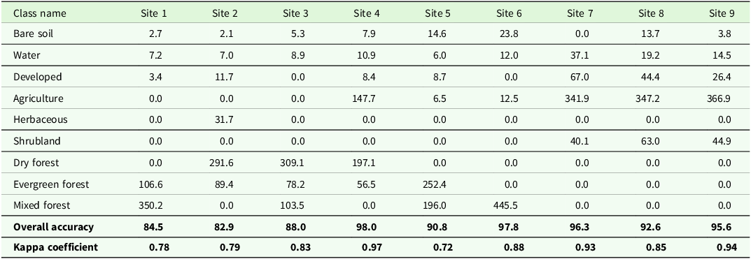
LULC classes included—(i) bare soil, (ii) water, (iii) developed area (and infrastructure), (iv) agriculture, (v) herbaceous land, (vi) shrubland, (vii) dry forest and savannas, (viii) evergreen forest, and (ix) mixed forest (Table 2, Figure 7). Sites ranged from agriculture dominant (site 7) to forest dominant (sites 1, 2, and 3), and to agriculture patches mosaiced within the forest matrix (site 4) (Table 2, Figure 7). Overall accuracy ranged between 82.9% and 98% and kappa coefficient ranged between 0.72 and 0.97 (Table 2). In terms of specific land use classes, the mean producer’s accuracy, i.e., how accurately real-world features can be classified, was the lowest for evergreen forest (68.37% ± 19.50), and the highest for water (96.14% ± 6.37) (Table S10). User’s accuracy, i.e., probability that a classified pixel on map would represent the same feature on the ground was the lowest for evergreen forest (78.12% ± 15.24) and the highest for the agriculture (96.53% ± 3.32) (Table S10).
Area (in ha) under different LULC classes calculated for 1 km buffer of the sampled segment
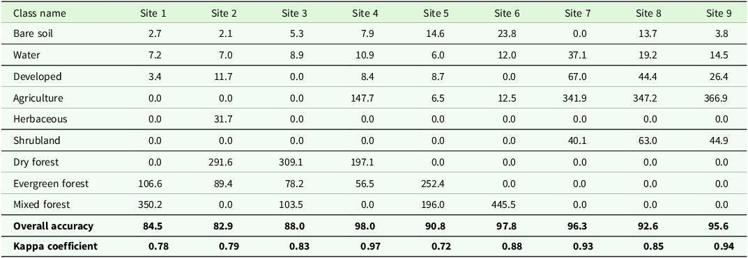
Table 2. Long description
The table presents the area in hectares under different land use and land cover (LULC) classes calculated for a 1 km buffer of sampled segments across nine sites. The table has 11 rows and 10 columns. The rows are labeled with LULC classes: Bare soil, Water, Developed, Agriculture, Herbaceous, Shrubland, Dry forest, Evergreen forest, Mixed forest, Overall accuracy, and Kappa coefficient. The columns are labeled with Site numbers from Site 1 to Site 9. Each cell contains the area in hectares for the corresponding LULC class and site. Notable trends include high values for Agriculture at Sites 7, 8, and 9, and significant areas of Evergreen forest at Sites 1, 2, 3, and 5. The Overall accuracy ranges from 82.9 percent to 98 percent, and the Kappa coefficient ranges from 0.72 to 0.97.
Land use and land cover classes within the 1 km buffer of surveyed river segments.

Figure 7. Long description
Panel A: A circular diagram showing a mix of land cover classes including bare soil, water, developed areas, herbaceous vegetation, agriculture, shrubland, dry forest, evergreen forest, and mixed forest. The river is prominently visible in blue. Panel B: A circular diagram highlighting developed areas in red, herbaceous vegetation in green, and water in blue. Panel C: A circular diagram emphasizing agriculture in orange, shrubland in brown, and water in blue. Panel D: A circular diagram focusing on dry forest in light green, evergreen forest in dark green, and water in blue. Panel E: A circular diagram showing a mix of land cover classes with a focus on bare soil in pink and water in blue. Panel F: A circular diagram highlighting developed areas in red and water in blue. Panel G: A circular diagram emphasizing agriculture in orange and water in blue. Panel H: A circular diagram focusing on shrubland in brown and water in blue. Panel I: A circular diagram showing a mix of land cover classes with a focus on dry forest in light green and water in blue.
Metrics and indices for river health
Index of Biotic Integrity
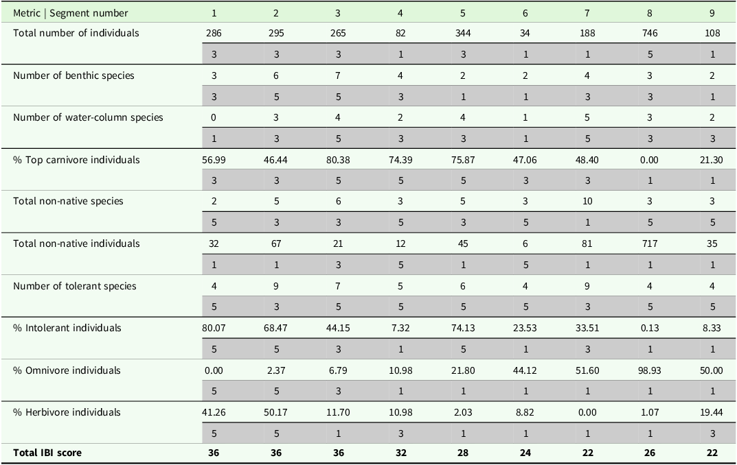
The scores for IBI ranged from 22 to 36 out of the total score of 50 (Table 3). The upstream segments (PA) scored higher than those downstream (NPA), indicating a change in fish community composition and decreasing integrity downstream. Further, PA segments had a higher percentage of intolerant individuals (habitat specialists) than NPAs but almost the same percentage of non-native individuals as in NPAs (Table 3). NPAs showed a higher number of omnivores and fewer herbivores. The percentage of top carnivore individuals dropped downstream of Kodiveri dam (NPA), which also contributes to an overall low score in NPAs (Table 3).
Absolute values for metrics, scores (in grey cells) and total scores for fish based IBI across the studied segments. Segment 1 to 6 are PAs and 7 to 9 NPAs

Table 3. Long description
The table presents absolute values for various metrics and scores related to fish-based IBI across nine segments. The segments are labeled from 1 to 9, with segments 1 to 6 being PAs and segments 7 to 9 being NPAs. The table includes the following columns: Segment number, Total number of individuals, Number of benthic species, Number of water-column species, % Top carnivore individuals, Total non-native species, Total non-native individuals, Number of tolerant species, % Intolerant individuals, % Omnivore individuals, % Herbivore individuals, and Total IBI score. Each row corresponds to a segment and lists the values for each metric. Notable trends include higher IBI scores in upstream segments (PAs) compared to downstream segments (NPAs), indicating a change in fish community composition and decreasing integrity downstream. PA segments have a higher percentage of intolerant individuals and a similar percentage of non-native individuals compared to NPAs. NPAs show a higher number of omnivores and fewer herbivores. The percentage of top carnivore individuals drops downstream of Kodiveri dam (NPA), contributing to an overall low score in NPAs.
Bird Integrity Index
Only four of the 13 metrics showed either a positive or negative trend with disturbance index D3 based on the plots, but these were not statistically significant (Figure S3, Table S11). These four metrics were total species richness (positive), percentage omnivore richness (negative), percentage shrub and bush nesting richness (negative), and percentage tree and shrub nesting richness (negative). A valid BII could not be computed since the metrics did not have a statistically significant response to disturbance. Ignoring the statistical significance and using these four metrics for BII, we found the index values to range from 0.98 to 2.67 (Table S12). Again, PAs scored higher than NPAs, and the lowest score was observed for the site downstream of the Kodiveri dam (Table S12). BII, however invalid, showed a decline in values moving downstream from PAs to NPAs (Table S12). At the reach scale, we found that none of the 44 metrics were correlated and did not show any relationship with disturbance indices D1, D2, and D3.
QBRc
QBRc values at reach scale ranged between 15 and 100 (Figure 8). Majority of NPA reaches scored negative for the first three components of QBRc, i.e., total riparian cover, cover structure, and cover quality, but positive for the fourth component, i.e., channel alteration. Only two reaches in PAs showed a QBRc score of less than 50. At the segment scale (averaged reach values), NPAs again scored the lowest (25), and the highest scores (87) were observed for PAs (Figure 8). 44% (n = 4) sites (or segments) had high values between 81 and 100, 22% (n = 2) sites had moderately high values between 61 and 80, and all NPA sites (33% of total sites) had low values between 21 and 40 (Figure 8).
QBRc scores of reaches sampled. Numbers in brackets, next to segment name show distance from starting point in metres. Grey bars represent NPA reaches. Points represent averaged segment values.

Figure 8. Long description
Panel A: A bar graph comparing QBRc scores of different reaches sampled. The horizontal axis lists the names of the segments with distances from the starting point in meters in brackets. The vertical axis represents QBRc scores ranging from 0 to 120. Grey bars represent NPA reaches, and points represent averaged segment values. The graph shows variations in QBRc scores across different segments, with some segments having higher scores and others lower. Notable trends include peaks and troughs in the scores, indicating varying health and ecological integrity of the riparian zones.
Riparian Strip Quality Index
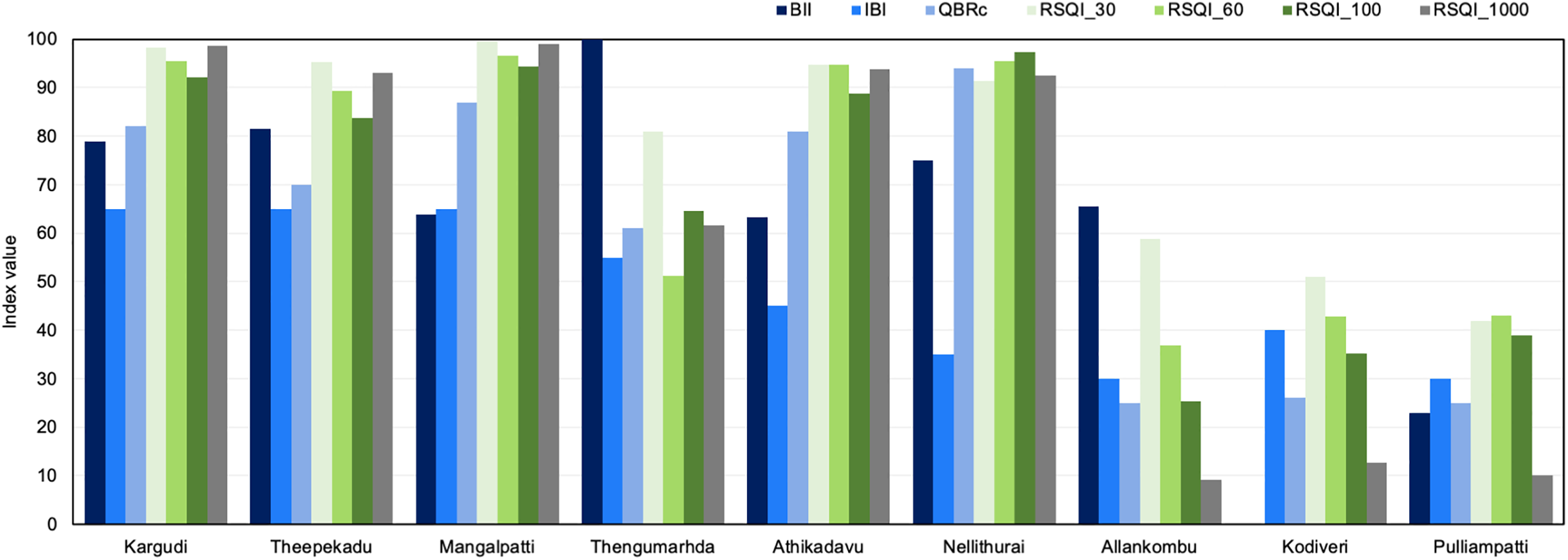
NPAs consistently had lower RSQI values compared to PAs across the four spatial buffers (30 m, 60 m, 100 m, and 1 km) (Figure 9). NPAs also showed a continuous decreasing trend as the buffer distance increased, which was not observed for PAs (Table S13). The RSQI values (RSQI_30) ranged between 41.8 (site 9, NPA) and 99.6 (site 3, PA) (Table S13). The values decreased for the 60 m buffer (RSQI_60) for all sites, ranging between 36.9 (site 7, NPA) and 96.6 (site 3, PA) (Table S13). For the 100 m buffer (RSQI_100), the lowest value was observed for site 7 (25.2, NPA) and the highest was for Site 6 (97.4, PA) (Table S13). RSQI was very low within 1-km buffer (RSQI_1000) for the NPA sites 7–9 (mean ± S.D., 10.6 ± 1.78), compared to the PA sites 1–6 (mean ± S.D., 89.8 ± 14.07).
Values of indices scaled between 0 and 100, for the sampled segments.

IBI correlated with RSQI at two scales. RSQI_30 and RSQI_1000 showed strong positive correlation with IBI (r = 0.85, p = 0.004; r = 0.84, p = 0.004, respectively) (Table S14). Interestingly, IBI did not show correlation with another field-measured index QBRc, but did with satellite-based index RSQI. On the other hand, QBRc correlated at all buffer widths with RSQI. It had strong positive correlation with RSQI_30 (r = 0.79, p = 0.012), RSQI_60 (r = 0.94, p = 0), RSQI_100 (r = 0.97, p = 0) and RSQI_1000 (r = 0.83, p = 0.006) (Table S14). BII did not show correlation with any other index. All three disturbance indices (D1, D2, D3) had negative correlation with QBR and RSQI.
Comparing the sites based on individual indices (Figure 9), we found that IBI and BII could not differentiate between PA and NPA segments, but QBR and RSQI computed for all four buffers showed a statistically significant difference (Mann–Whitney U test, ɑ = 0.05).
Discussion
General trends
In this study, we incorporated representative taxa for terrestrial and the land-water transition zone into river health assessment. Traditionally, this has been missing in Indian studies which are usually limited to fishes or micro-and macro-invertebrates (Bhat Reference Bhat2017; Das and Samanta Reference Das and Samanta2006; Ganasan and Hughes Reference Ganasan and Hughes1998; Nair et al. Reference Nair, Muhammadali, Koushlesh, Chanu, Das, Bhakta, Pillai, Gogoi, Samanta, Meetei, Baitha, Kamble, Kumar and Das2023; Sajina et al. Reference Sajina, Sudheesan, Samanta, Paul, Bhowmick, Nag, Kumar and Das2022). Overall, all four indices showed a decline in values as we moved downstream in the Moyar and Bhavani Rivers. This was expected because downstream segments have high human population density which might directly or indirectly altered the riparian habitats and its associated biodiversity (Adeola Fashae et al. Reference Adeola Fashae, Fatayo and Olusola2023; Castro-López et al. Reference Castro-López, Guerra-Cobián and Prat2019). This was also noted in the LULC maps showing a transition from forest-based landscape to agricultural landscape.
For IBI, the total score declined moving downstream, but the individual metrics changed differently. Therefore, these metrics are useful individually in informing local fisheries and wildlife management (Hughes and Oberdorff Reference Hughes, Oberdorff and Simon1998). For example, the total abundance was very low in the two PA segments (4 and 6), which can be investigated locally. In another instance, the non-native species of fishes (not native to Western Ghats) were particularly high downstream of Kodiveri dam (segment 8, 9), likely because of introductions by the Tamil Nadu State Fisheries Department. The species richness was also low downstream of the Kodiveri dam, which could be due to low water depth (0.46 ± 0.25 m) and low channel width (18.00 ± 3.12 m) which resulted from water diversion supporting only bottom and mid-column feeders like Dawkinsia filamentosa, Garra stenorhynchus and Oreochromis mossambicus.
There is a general lack of long-term data for the fish populations, and their changing composition except for a few snapshots. From the previous studies, we found two sets of observations with some overlap in the study area—one from Rajan (Reference Rajan1963), who observed 28 fish species in the Pykara and Moyar Rivers, but almost 19 of these species were not observed in our study. Second, a study by Arunkumar et al. (Reference Arunkumar, Sivaraman and Manimekalan2017), who observed three Puntius species at Nellithurai (other sites cannot be compared), and we observed two species upstream and one downstream of this site.
The trends noted for the four bird metrics that responded to disturbance, however insignificant, can be explained through field observations and known habitat preference of the species. The total bird richness was found to increase with disturbance. Open habitats (NPAs) were more disturbed but also offered heterogeneous habitats, e.g., nearby croplands and human habitation, compared to the closed canopy sites in the PAs (Panda et al. Reference Panda, Prusty, Panda, Pradhan and Parida2021). Some groups, especially the herons, ducks, and geese, were more frequently sighted in open habitats, increasing the bird species’ richness and abundance. Other factors influencing this could be the bush cover on the banks, water flow and depth, positively aligning with species preference. The other three metrics, percentage omnivore richness, percentage shrubs and bush nesting richness, and percentage tree and shrub nesting richness all declined with increasing disturbance. The latter two represent specialist species groups, and since the NPAs had poor vegetation cover (particularly of trees and shrubs), these segments offered fewer nesting choices to the birds. Among the omnivores were commonly occurring species like Common Babbler, Coppersmith Barbet, Great Tit, House Crow, Indian Peafowl, Jerdon’s Leafbird, Jungle Myna, Loten’s Sunbird, Purple-rumped Sunbird which prefer tree cavities, shrubs, bushes, thickets, and man-made structures (Table S5). Overall omnivore richness declined with disturbance but was the highest in two disturbed segments (Theppekadu and Allankombu).
QBRc values, especially at reach level, suggest that there are degraded reaches with poor riparian cover interspersed between good quality reaches. This is confirmed by RSQI and negative relationship of both QBRc and RSQI with disturbance index. Both QBRc and RSQI allocate higher scores to good riparian cover and forests and penalize agriculture and infrastructure. Therefore, this relationship was expected. Other studies surprisingly found either weak or no correlation between the two indices or did not test for it (Machado and Kim Reference Machado and Kim2024; Rivas-Fandiño et al. Reference Rivas-Fandiño, Acuña-Alonso, Novo, Pacheco and Álvarez2023; Saha et al. Reference Saha, Das, Dasgupta and Patel2020).
Protected riparian areas are ‘healthier’ than non-protected areas
We compared the segments in PAs and NPAs, assuming the less disturbance in PAs would reflect in the indices of riparian health. Among the four indices, both QBR and RSQI were able to differentiate between PAs and NPAs, indicating a degraded state in the latter. Some studies have supported this hypothesis finding a higher species richness or better water quality in protected streams, compared to the unprotected streams (Kantharajan et al. Reference Kantharajan, Yadav, Chandran, Singh, Mohindra, Krishnan, Kumar, Shukla and Lal2022; Lovegrove et al. Reference Lovegrove, Dreyer and Le Breton2025; Valentim et al. Reference Valentim, Feio and Almeida2024) and others (Abraham and Kelkar Reference Abraham and Kelkar2012; Gupta et al. Reference Gupta, Sivakumar, Mathur and Chadwick2015; Sarkar et al. Reference Sarkar, Pathak, Tyagi, Srivastava, Singh and Dubey2013) have found positive impacts of protection on fish species richness and diversity. BII also had the lowest values in the NPAs, but no clear pattern emerged. It must be noted that BII was not based on a statistically significant metric-disturbance relationship; therefore, its consideration requires caution.
Some of the variation in values of the indices can be attributed to differences in vegetation and canopy cover in PAs and NPAs. The Moyar River passes through forested and protected areas, where canopy cover is high and riparian vegetation is less disturbed, compared to the Bhavani River, where the riparian cover is limited to scattered shrubs and trees with agriculture or human habitation on riverbanks. And while PA segments scored higher than NPAs for QBR and RSQI, these were not completely devoid of disturbance and require management interventions. Some reaches in PAs were disturbed due to invasive species such as Prosopis juliflora, and Eicchornia crassipes, animal grazing, major roads, and release of wastewater, which reflected in low QBR scores and high disturbance scores (Prasetyo et al. Reference Prasetyo and Ramadhan2021).
A recent global review has found mixed impacts of PAs on aquatic ecosystems, and the conditions under which PAs fail or succeed remain unknown because of lack of comparable and appropriate study designs and limited datasets (Acreman et al. Reference Acreman, Hughes, Arthington, Tickner and Dueñas2020). Considering the IBI values, the quality of habitat declined in some protected forest segments and showed declining health downstream of segment 4 (Thengumarhda). Downstream of site 6 (Nellithurai) there is a change in trend where the riparian areas degrade but have comparatively better scores for IBI (IBI > QBR).
Overall, there were more native fishes in PAs than in NPAs such as Garra stenorhynchus, Devario malabaricus, and Opsarius gatensis, with the exception of Dawkinsia filamentosa. Abraham and Kelkar (Reference Abraham and Kelkar2012) obtained similar results for the streams in the Kerala region of the Western Ghats. Percentage of benthic species was also the highest in the protected segments, suggesting good habitat quality. Further, high abundance of omnivores in the Bhavani River (and NPAs) (Das and Samanta Reference Das and Samanta2006), and high abundance of intolerant individuals in the Moyar River (PA), suggests that there are more specialists in PAs compared to NPAs (Britton et al. Reference Britton, Day, Doble, Ngatunga, Kemp, Carbone and Murrell2017). Das and Samanta (Reference Das and Samanta2006) also found more tolerant species in the stressed sites compared to the reference sites in the Hooghly River estuary in the state of West Bengal. However, given the sample size, our observations may not hold true at the regional scale. Nonetheless, there is a need for community-focussed habitat management, especially in sites where specialists are abundant.
Water quality assessments add informative data to the biological indices
The results from metrics and indices were complemented by water quality parameters. We found that although PA segments scored high for biological indices, their water quality cannot be assumed to be good. Some segments in the Moyar and Bhavani Rivers had DO levels less than 6.5 ppm, which is considered unfit for aquatic life (Chapman Reference Chapman1996). This could be due to the low velocity which did not allow mixing of oxygen. Further, there are both point and non-point sources of pollution throughout the studied stretch but since we did not test for biological oxygen demand, we cannot assume if low DO was contributed by the sewage discharge.
Comparison with previous studies shows that water quality values vary considerably within an observation period, and therefore, there is a need for frequent and widespread monitoring stations. For example, between segment 6 (Nellithurai) and the Bhavanisagar dam, Sivakumar et al. (Reference Sivakumar, Prasanthrajan, Shalini and Balaji2018) found that dissolved oxygen varied between 2.36 and 8.87 mg L−1 and electrical conductivity ranged between 0.06 and 1.59 dS m−1, during the June–September period. In another study (Varunprasath et al. Reference Varunprasath and Daniel2010), at the sites near Nellithurai, values for DO range between 5.5 and 8.4 mgL−1, and EC between 180 and 1400 mMho, showing that elsewhere in the Moyar and Bhavani Rivers, DO levels drop to less than 6 ppm. In the Bhavani River, there are industries upstream of the Bhavanisagar dam and it also receives municipal wastewater from major towns, which could be one of the factors causing the NPA segments 6, 7 and 8 to have low DO values (Prasanthrajan et al. Reference Prasanthrajan, Suseendranath, Shalini and Duraibabu2018).
We observed that in addition to the natural rainfall-related high discharge, all the sites experienced a noticeable fluctuation in water discharge due to release of water from dams. The Moyar hydroelectric dam and several check dams affected water discharge in all the sampled segments of the Moyar River. This region is in a rain shadow area, and while rainfall in the sampled region was low, rainfall in upstream areas contributed to the high discharge. River width, on the other hand, generally increased with increasing river order and downstream (as described under RCC by Doretto et al. Reference Doretto, Piano and Larson2020), but this trend was also disrupted because of water diversion at the Bhavanisagar and Kodiveri dams.
Bird metrics and invalidity of BII
While computing BII, we found that four metrics responded to disturbance scores but showed no significant trends, which could be due to small sample size. But at the reach scale involving 44 reaches, we found no correlation among the bird metrics which limited further analysis. Due to insignificant relationships of the metrics with disturbance index, we suggest that other approaches of computing a bird-based index need to be explored. In an alternate approach, habitat specialists such as the Black bittern, Black crowned night heron, Grey-headed fish eagle, and the Malabar Whistling Thrush could be used as indicators of river health, as tested elsewhere in India (Sinha et al. Reference Sinha, Chatterjee, Ormerod, Adhikari and Krishnamurthy2019). Their presence, however, was limited to one or two segments, which warrants a systematic search for indicator species for this region.
Limitations and future scope
Multi-metric or integrated indices have both advantages and disadvantages, which have been widely discussed (Capmourteres et al. Reference Capmourteres, Rooney and Anand2018; Gippel et al. Reference Gippel, Zhang, Qu, Bond, Kong, Leigh, Catford, Speed, Meng, Hart and Doolan2017; Jarvie and Jackson Reference Jarvie and Jackson2023; Monaghan Reference Monaghan2016; Seegert Reference Seegert2000). Some of these limitations are their sensitivity to scale, variability in sampling methods, sampling errors, and changes in community composition in different years. Further, the taxa studied can show spatio-temporal variation in sensitivity/response to the stressor. The stressors may also change across the landscape affecting different species, and some of these stressors can be complex to quantify. Some of these attributes can only be quantified when this approach is scaled up. We could limit some of the bias and errors by fixing the observers and sampling times for the sites, the seasonal variability could not be assessed. The study could benefit from observations across different seasons to understand how the metric values vary with changes in water levels, discharge, bank vegetation and agricultural practices (Machado and Kim Reference Machado and Kim2024). Another limitation of this approach is that sampling is restricted to the segments where riverbanks are walkable and channels are wadable. Some reaches had to be avoided because they had steep slopes or difficult terrain or they were part of private property. Some of these limitations are also reported by Bryce et al. (Reference Bryce, Hughes and Kaufmann2002). Additionally, we could not collect data for riverbed material in some reaches due to high water discharge from the dam, which made it unsafe for sampling. Similarly, some forest sites were unsafe to sample during early hours because of elephant movement. However, all bird surveys were conducted at the same time in each segment to reduce bias. Collectively, these limitations may have resulted in the under-recording of certain species, especially seasonal migrants and elusive taxa.
Further, our sampled segments are part of a ‘discontinuous’ river stretch which is impacted by the tributaries, check dams and reservoirs (Doretto et al. Reference Doretto, Piano and Larson2020). In recent times, ecologists are seeing rivers as dendritic networks, with tributaries and reaches as branches, and confluences, dams, and lakes as nodes (Altermatt Reference Altermatt2013). Accordingly, the position of a reach or segment within the dendritic network of streams affects the biotic community composition and their migration (Altermatt Reference Altermatt2013; Doretto et al. Reference Doretto, Piano and Larson2020; Henriques-Silva et al. Reference Henriques-Silva, Logez, Reynaud, Tedesco, Brosse, Januchowski-Hartley, Oberdorff and Argillie2019). An extensive sampling would likely reveal the effects of such discontinuities which could not be quantified given the scope of this study.
There is no single index that can inform the riparian health or integrity without limitations, as noticed in our study and in others. Some of the limitations are inherent in how the indices have been designed. For example, RSQI has other shortcomings that warrants its use with other indices. First, it cannot detect any disturbances and infrastructure below the canopy or those smaller than the image spatial resolution (Rivas-Fandiño et al. Reference Rivas-Fandiño, Acuña-Alonso, Novo, Pacheco and Álvarez2023). For example, we detected camp-fires and ferries during field surveys, which would have been missed otherwise. Second, availability of cloud free images of coastal regions is limited to a few days in a year. This combined with limited spectral resolution can affect the ability to distinguish between vegetation types, affecting classification accuracy. Third, it cannot differentiate between the native and non-native or invasive species (Rivas-Fandiño et al. Reference Rivas-Fandiño, Acuña-Alonso, Novo, Pacheco and Álvarez2023); consequently, a forest dominated by invasive shrubs would still receive a weight of 10, as observed in many forest patches in this region (Chaitanya Reference Chaitanya2025; Sivakumar Reference Sivakumar2024). Computing RSQI is comparatively easy and can be part of a rapid river monitoring framework. This would complement indices like IBI, QBR, and water quality assessments. In India, however, the absence of a country-wide, high-resolution LULC map, necessitates a mapping exercise.
We did not use any reference segment for comparison in this study. While the Moyar is a comparatively less disturbed river compared to the Bhavani, and passes through a protected area, it is prone to disturbance from elephant washing and the release of domestic sewage generated from small towns such as Theppekadu. Due to lack of systematic data, we could not select a reference segment within the Moyar River. For larger extents, however, it might be useful to designate reference segments and set thresholds for river health classification and the resulting management plans. The criteria for designation of a reference site in Indian studies are usually the selection of the least disturbed site, where the definition of ‘disturbed’ varies across studies and depends on the context. Das and Samanta (Reference Das and Samanta2006), when sampling six sites in the Hooghly estuary for IBI, designated two upstream sites which did not have any point source of pollution, as the reference sites. Bhat (Reference Bhat2017) classified sites as disturbed and undisturbed based on human footprint and then used the least disturbed site as a reference. Sajina et al. (Reference Sajina, Sudheesan, Samanta, Paul, Bhowmick, Nag, Kumar and Das2022) used water quality index to designate polluted or stressed sites and tested for correlation between IBI and the water quality index. In our case, if we combine information from the three indices (ignoring BII), segment 1 (Kargudi) appears to be the least disturbed but has low values for dissolved oxygen and oxidation-reduction potential. However, the unsatisfactory water quality could be temporary or seasonal and needs to be explored further.
This approach could be tested for other sites in similar landscapes and has the potential to be incorporated into regular monitoring exercises, such as those developed for tiger and elephant census. This could be done with working partnerships between local universities, research institutes, NGOs, volunteer networks and the State Forest Department. This partnership is also expected to provide a space to discuss management goals and objectives, including the usefulness of the indices which might differ among the stakeholders. Successful implementation will require some training for species identification, data recording, and analysis in the initial years. Species identification is crucial since the index values rely on accurate species identification. Training and discussions with local fishermen will be helpful to gather additional data about disturbances and changes in their daily catch. Since the electrofishing method is not permissible in India, regular monitoring with traditional fishing gear (cast net, bamboo traps, hook, and line methods) relies on the expertise of the fishermen and could prove to be a mutually beneficial partnership.
Conclusion
We tested four indices for riparian health in the southern Indian perennial streams. IBI, RSQI, and QBRc showed a decline in values downstream from PA to NPA areas. When assessed at reach level, QBRc scores reflected poor habitat quality along some reaches of PAs. We found that IBI, RSQI, and QBR could be easily adapted and provided important information about the riparian condition. For a comprehensive riparian zone profile, these indices could be used together with the water quality and hydrology data to inform conservation and management. Bird index could not be adapted, and bird metrics did not show clear patterns with the disturbance index. For bird-based assessment of river health, alternate approaches need to be investigated. Our study serves the dual purpose of providing the baseline data for these taxa and adaptation of the selected indices.
Supplementary material
The supplementary material for this article can be found at https://doi.org/10.1017/S0266467426100650.
Acknowledgements
We thank Wildlife Institute of India and Tamil Nadu Forest Department for their support and cooperation for this study, especially the Divisional Forest Officer of Erode Mr. S. Gowtham, Mr. Ashok Kumar, Divisional Forest Officer, Coimbatore, Mr. Kiruba Shanker, Deputy Director, Sathyamangalam Tiger Reserve, and Mr. Senthil Kumar, Assistant Conservator of Forests, Coimbatore Forest Division. We extend thanks to Ms. Divya, Forest Range Officer – Karamadai, Mr. Sivakumar, Forest Range Officer – Bhavanisagar, Mr. Mani Venkatesh, Forest Range Officer – Thengumarhada, Mr. Manoj Kumar, Forest Range Officer – Mudumalai, Mr. Joseph Stalin, Forest Range Officer – Mettupalayam, with whom we were able to coordinate our field visits and safely conduct research. We also thank the supporting team of researchers, trackers and fishermen without whose support this information could not have been collected. We thank Alljo Paul (Project Associate, Wildlife Institute of India), Meera Makwana (Project Associate, Wildlife Institute of India), Sneha Gupta (Project Intern, Wildlife Institute of India), Kavin D. (Salim Ali Centre for Ornithology and Natural History), Vijayan (Elephant Tracker, Indian Institute of Science), M. Kunmari (Elephant Tracker, Indian Institute of Science), Meen Kaalan (Anti-Poaching Staff, Mudumalai Tiger Reserve), Magesh (Anti-Poaching Staff, Sathyamangalam Tiger Reserve), S. Vadugan (Anti-Poaching Staff, Karmadai Forest Range), Nagan (Forest Watcher, Nilgiri Forest Division), Rangan (Fisherman, Thengumarhda), Suresh (Fisherman, Thengumarhda), Shankar (Fisherman, Thengumarhda), Arun Kumar (Fisherman, Kodiveri), Palzanichami (Fisherman, Mettupalayam).
Funding support
This study was conducted with funding support available to VA under the Long Term Ecological Observatories (LTEO) project by the Ministry of Environment, Forest and Climate Change, Government of India, and to RK from the ongoing project of Wildlife Institute of India, supported by the National Tiger Conservation Authority, Government of India.
Competing interests
Authors declare that they have no competing interests.
Research permission
For this study, research permission was received from the Principal Chief Conservator of Forests and Chief Wildlife Warden, Chennai (No. WL5(A)/29674/2021, dated 26.03.2022) and Field Director, Mudumalai Tiger Reserve, Udhagmandalam (Ref. No. 2920/2022-P1, dated 30.06.2022) for data collection in protected areas.
Ethical statement
The authors assert that all procedures contributing to this work comply with applicable national and institutional ethical guidelines on the observation and handling of wild animals.









 Open access

