




No CrossRef data available.
STOCHASTIC MARKET EQUILIBRIUM MODEL FOR GENERATION PLANNING
Published online by Cambridge University Press: 31 August 2005
Abstract
It is widely accepted that medium-term generation planning can be advantageously modeled through market equilibrium representation. There exist several methods to define and solve this kind of equilibrium in a deterministic way. Medium-term planning is strongly affected by uncertainty in market and system conditions; thus, extensions of these models are commonly required. The main variables that should be considered as subject to uncertainty include hydro conditions, demand, generating units' failures, and fuel prices. This paper presents a model to represent a medium-term operation of the electrical market that introduces this uncertainty in the formulation in a natural and practical way. Utilities are explicitly considered to be maximizing their expected profits, and biddings are represented by means of a conjectural variation. Market equilibrium conditions are introduced by means of the optimality conditions of a problem, which has a structure that strongly resembles classical optimization of hydrothermal coordination. A tree-based representation to include stochastic variables and a model based on it are introduced. This approach to market representation provides three main advantages: Robust decisions are obtained; technical constraints are included in the problem in a natural way, additionally obtaining dual information; and large-size problems representing real systems in detail can be addressed.
Information
- Type
- Papers from the 8th International PMAPS Conference
- Information
- Probability in the Engineering and Informational Sciences , Volume 19 , Issue 4 , October 2005 , pp. 533 - 546
- Copyright
- © 2005 Cambridge University Press
1. INTRODUCTION
A new framework of competitive generation markets has arisen in a large number of countries, requiring the development of new operation and planning tools to aid in the decision task traditionally made by tools designed for a centralized environment. One of these strategic tasks is the medium- and long-term hydrothermal coordination that is being commonly addressed in deregulated environments by finding a Nash equilibrium. The equilibrium point is defined as a set of prices, generator outputs, consumption, and other relevant numerical quantities, which no market agent could modify unilaterally, by changing its behavior, without a decrease in its profit.
Different methods have been suggested to compute this equilibrium. It is possible to find it by maximizing a profit function for one agent if some restrictive assumptions are accepted [1,14]. Other alternatives include game theory [5], iterative methods based on a representation of the bidding process [10], or genetic algorithms [9]. As the market equilibrium is mathematically characterized by a set of equations and inequalities that include the so-called complementary conditions, it has been proposed to deal with this issue using such techniques as heuristics [3], the linear complementary problem [7,12], and the inclusion of equilibrium constraints [13]. These approaches are characterized by their complexity.
The focus used in this paper to solve equilibrium market is different from previous ones. The market is represented using a conjectural variation approach. The adjustment of production that generator companies will produce as a response to a price variation is assumed to be linear and known [4]. It is possible to show that, under some reasonable assumptions, the solution of the market equilibrium conditions is equivalent to the solution of a minimization problem with a structure that strongly resembles classical optimization of hydrothermal coordination [2].
This paper extends this market equilibrium representation technique to allow for the consideration of uncertainty in some of the market conditions. The structure of the optimization problem is suitable to fit in stochastic representations for the operation of hydrothermal generation systems [6,8,11].
Five main sources of uncertainty can be identified when it comes to medium-term generation operation: hydro inflows, fuel prices, system demand, generating units' failures, and competence behavior. Any of these factors can be considered as stochastic, with the proposed focusing based on a scenario tree representation. The proposed model is especially interesting from a practical point of view because it is able to compute robust decisions for large-size systems, including a detailed description of the technical characteristics of the system that determine the shape of the agents' cost functions.
In Section 2 the deterministic case for market equilibrium computation by optimization is summarized and generalized for the stochastic case; Section 3 presents a study case that shows the model capabilities. The main conclusions are stated in Section 4.
2. STOCHASTIC EQUILIBRIUM COMPUTATION
2.1. Deterministic Market Equilibrium
In [2], medium-term market equilibrium was defined from a deterministic point of view. It was proved that under some reasonable assumptions, it can be formulated as an equivalent minimization problem. This result is summarized herein in a simplified version, for a single unitary period and without contracts signed by generation companies.
Let us assume a generation market in which offers are a linear function of price:

Pi is the offered power by generation company i, λ is the demanded price, and Pi0 and αi are two constants that characterize the linear offer. Let us also assume that demand can be described by

where D0 is the intercept of the demand, which is assumed to be known, and α0 represents the demand slope.
Given Pi0, αi, D0, and α0, the market clearing price λ, generated powers Pi, and demand D are computed by solving the system formed by (1) and (2) and the generation–demand balance equation:

In order to compute its offer (i.e., the Pi0 and αi coefficients), each generation company must make some assumptions on the offers that the other utilities are going to send (i.e., it must have some idea on the coefficients Pj0 and αj, j ≠ i). For each particular assumption on these coefficients, there is a residual demand function (4). Note that the sum of αj, where i ≠ j, includes α0

Given this function, companies' offers must maximize their profit, which is assumed to be

The first term represents the market income and the second one represents the production cost. By differentiating and zeroing,

Equations (2), (3), and (6) constitute a Nash market equilibrium that can be obtained from the solution of the minimization problem:

The effective cost functions Ci(Pi) are defined as

The utility function U(D) is defined as

The clearing price λ is the Lagrange multiplier of the constraint (3).
2.2. Scenario Tree Definition
If some of the parameters included in the previous representation of market equilibrium are considered to be subject to uncertainty, the approach has to be extended. A basic alternative is taking it into account in analyzing a set (normally a reduced set, due to the size of the problem) of representative scenarios. Market equilibrium is computed for each of them separately. Results obtained from these scenarios are analyzed together. The main drawback of this method is its lack of robustness for short-term operation: Different decisions are obtained for the first time period in each scenario. Additionally, the reduced number of scenarios does not make the analysis accurate enough if treated as a Monte Carlo simulation.
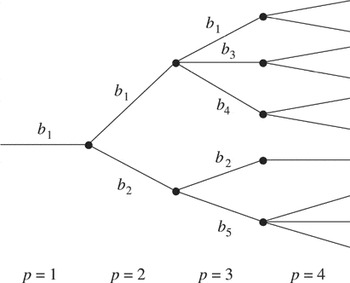
A more advanced possibility to include uncertainty, especially when the size of the problem prevents an extensive Monte Carlo analysis, is using a scenario tree. It has the main advantage of allowing one to include stochastic variables and to compute a single robust decision for the first period of the study. A sample tree is shown in Figure 1. Periods are numbered consecutively and branches are also numbered consecutively starting with b1 within each period.

Sample scenario tree.
Tree structure is established using a correspondence and a set. The correspondence a(p,b) relates the branch b of period p with the one that is immediately before it. The set B(p) includes all the branches that are defined in period p. In the tree in Figure 1, for example, a(p3,b5) = b2 and B(p3) = {b1,b2,b3,b4,b5}.
A probability wpb is defined for each branch. To guarantee tree coherence, the total probability of the branches in a period must add to one:

In addition, the probability of all the branches following a single one must include the probability of the previous branch:

The use of a scenario tree implies that the definition of an objective function is maximized along the whole tree for every agent in the market. In this paper, the mean profit is used; it is defined as

This expression includes the duration of each period, lp. Alternative objective functions could be defined, including those nonneutral to risk modifying the value of probabilities.
This new definition of profit implies that prices, companies' productions, or costs may be different for each branch tree. The use of different cost functions for each branch tree allows a probabilistic representation of any parameter that affects these costs, such as fuel costs, hydro inflows, or the units' availability.
2.3. Stochastic Market Equilibrium Definition
The previous market representation requires an extension of the market equilibrium concept. First, offers have different slopes in each branch of the tree, representing different behaviors of the companies under different circumstances:

Additionally, demand is also different for each branch that can be used to introduce uncertainty in demand value:


Similar to the deterministic case (6), the maximization of the profit function for each company leads to

Equations (14)–(16) define the stochastic market equilibrium.
2.4. Stochastic Equilibrium Computation by Optimization
The newly defined equilibrium can be obtained from the solution of the following minimization problem that is a natural extension of the deterministic one:

The effective cost functions Cipb(Pipb) are defined as

The utility function U(Dpb) is defined as in (9):

The clearing price for each period and branch λpb is now obtained from the Lagrange multiplier of the constraint as follows:

Optimality conditions of the presented optimization problem are the same as equilibrium market equations. This can be easily shown for first-order conditions. The Lagrange function for the previous optimization problem is

The solution to the optimization problem is obtained by differentiating and zeroing this function:


These three expressions are equivalent to those that define market equilibrium. Equation (22) corresponds to (15), the balance of generation and demand. Equation (23) is equal to (16), the market equilibrium condition, if price is computed using (20). Finally, (24), with the same price expression, leads to (14), the linear relationship between price and demand. Thus, stochastic market equilibrium can be computed by solving an optimization problem. A further analysis shows that second-order conditions are also the same for both formulations.
2.5. Inelastic Demand Representation
In some cases, demand can be treated as a known value for each branch and independent of price. If demand is inelastic, it can be easily shown that market equilibrium can be obtained as the solution to a simplified optimization problem:

2.6. Cost Functions Representation
The structure of the problem allows adding variables and constraints to represent the cost functions and the technical constraints related to it within the same optimization problem. To illustrate this point, the power system will be considered as a group of thermal and hydro units owned by different companies. The following new variables have to be included:

Generated power, as will be shown later, may be computed as a linear combination of decision variables.
Some additional parameters must also be considered. Hydro inflows have been assumed as stochastic and so they have a different value in each branch.

Generated power for utility i in branch b of period p is computed as a linear combination of decision variables.

The following constraints are added to the problem.
Decision variables bounds:


Power balance for each branch and period [the result of including (26) in (15)]:

Energy balance for each period, branch, and hydro unit:

Finally, the cost function can now be included explicitly in the objective function as a linear combination of decision variables, keeping the structure of the optimization problem:

3. STUDY CASE
3.1. System Description
This study case represents an operation in a market divided into nine periods representing January to September. It has been determined that hydro energy storage at the end of September is the lowest in the year and easy to forecast.
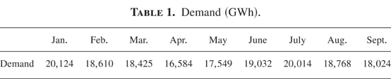
Table 1 shows demand, which has been considered inelastic.
Demand (GWh).

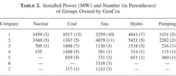
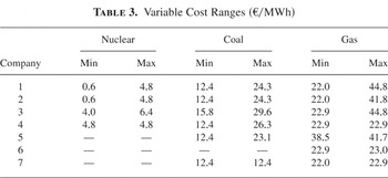
Seven generation companies are competing in the market. Table 2 shows its generation structure and Table 3 shows the ranges for variable costs. This case is an example of a real-size case and loosely represents the Spanish daily market, where a large number of groups is owned by a smaller group of companies. The model could be also used if the same set of groups was the property of a large number of companies.
Installed Power (MW) and Number (in Parentheses) of Groups Owned by GenCos

Variable Cost Ranges (€/MWh)

Conjectural variations have been assigned according to the company's size, ranging from 2.5 to 5.0 for the largest ones (companies 1, 2, and 3), between 1 and 2 for the medium-sized utilities (companies 4, 5, and 6), and a single value of 0.5 for the smallest one (company 7). Units for this parameter are euros per megawatt-hours per gigawatt.
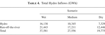
Three different scenarios have been considered for hydro inflows: wet, medium, and dry, with probabilities 0.1, 0.4, and 0.5, respectively. The highest probability for the worst case from the company's point of view (dry scenario leads to highest operation cost) represents a nonneutral to risk point of view. Table 4 shows total hydro inflows considered for each one.
Total Hydro Inflows (GWh)

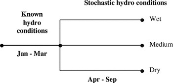
The structure of the tree is shown in Figure 2. The value of inflows is the same for the first three months; the rest of the year makes the difference. These three scenarios have been solved separately (considering a deterministic market equilibrium) and also together, solving a stochastic market equilibrium. The objective of this tree structure is to decide the operation for the first 3 months. Differences between deterministic and stochastic approaches will be studied. The model has been coded in GAMS 21.0 language and solved by using CPLEX 8.1 solver. The execution time for the presented case is about 15 min in a 1.7-GHz PC with a Pentium IV processor.

Scenario tree for study case.
3.2. Results
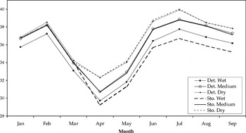
Prices are presented in Figure 3. Substantial differences appear between stochastic and deterministic analysis. Prices in dry and medium deterministic scenarios are similar to those in the dry and medium branches of the stochastic case. Shortage of hydro resources prevents companies from different hydro resources management. However, prices in the wet branch of the stochastic case are lower in comparison to the deterministic case because more hydro energy is stored in this case. Medium deterministic case and medium stochastic branch are very similar although these similar prices produce different hydro resources operation for the first time periods.

Prices for deterministic and stochastic cases (€/MWh).
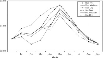
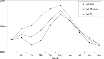
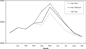
Energy reservoir levels are shown in Figure 4. For the sake of clarity, deterministic and stochastic reservoir levels have been represented separately in Figures 5 and 6.

Reservoir levels for company 2 for deterministic and stochastic cases (GWh).

Reservoir levels for company 2 in deterministic cases (GWh).

Reservoir levels for company 2 in stochastic cases (GWh).
The stochastic analysis suggests a more conservative resources management in order to face the dry scenario in the event that it would occur. In January, February, and March, a larger amount of hydro energy is reserved in the stochastic case than in the wet and medium deterministic cases.
The analysis of deterministic cases shows that management of the dry scenario is unrealistic. High reservoir levels are kept in order to take advantage of the high prices that will happen from June to September. This would not be a good decision if a wet scenario occurred in April (for example) and prices fell. In a similar way, the wet deterministic case is not realistic.
Decisions taken in the stochastic case for wet and dry branches are more robust because in this case, only 3 months of inflows are supposed to be known in advance.
4. CONCLUSIONS
A stochastic representation of market equilibrium has been introduced, including its equivalence with an optimization problem to solve it efficiently.
Market equilibrium has been represented by means of a conjectural variation and has been computed along a scenario tree that allows the inclusion of stochastic variables. A study case with stochastic inflows has been solved and analyzed showing this model's advantages. Other variables could have been considered as stochastic using the same method.
The previous features make this approach very interesting from a practical point of view: First, robust decisions are obtained; second, technical constraints are included in the market equilibrium representation in a natural way obtaining dual information; and third, large-size problems representing real systems with a large number of companies (or alternatively with a reduced number of companies owning a large number of groups each) can be addressed.
References
REFERENCES
Barquín, J.,
Centeno, E.,
Malillos, E., &
Román, J.
(1999).
Medium-term hydro operation in a competitive electricity
market.
IEEE International Conference on Electric Power Engineering
PowerTech.
Barquín, J.,
Centeno, E., &
Reneses, J.
(2004).
Medium-term generation programming in competitive environments: A
new optimization approach for market equilibrium computing.
IEE Proceedings—Generation, Transmission and
Distribution
151(1):
119–126.Google Scholar
Bushnell, J.
(1998).
Water and power: Hydroelectric resources in the era of competition
in the western US.
Power Conference on Electricity Restructuring, University of
California, Energy Institute.
Day, C.J.,
Hobbs, B.F., &
Pang, J.S.
(2002).
Oligopolistic competition in power networks: A conjectured supply
function approach.
IEEE Transactions on Power Systems
17(3):
597–607.Google Scholar
Ferrero, W.,
Shahidehpour, S.N., &
Ramesh, V.C.
(1997).
Transaction analysis in deregulated power systems using game
theory.
IEEE Transactions on Power Systems
12(3):
1340–1347.Google Scholar
Gorenstin, B.G.,
Campodonico, N.M.,
Costa, J.P., &
Pereira, M.V.F.
(1992).
Stochastic optimization of a hydrothermal system including network
constraints.
IEEE Transactions on Power Systems
7(2):
791–797.Google Scholar
Hobbs, B.F.
(2001).
Linear complementary models of Nash–Cournot competition in
bilateral and POOLCO power markets.
IEEE Transactions on Power Systems
16(2):
194–202.Google Scholar
Morton, D.P.
(1993).
Algorithmic advances in multi-stage stochastic programming.
Ph.D. thesis,
Stanford University, Stanford, CA.
Nguyen, D.H.M. &
Wong, K.P.
(2002).
Natural dynamic equilibrium and multiple equilibria of competitive
power markets.
IEE Proceedings—Generation, Transmission and
Distribution
149(2):
133–138.Google Scholar
Otero-Novas, I.,
Meseguer, C.,
Batlle, C., &
Alba, J.J.
(2000).
Simulation model for a competitive generation market.
IEEE Transactions on Power Systems
15(1):
250–256.Google Scholar
Pereira, M.V.F. &
Pinto, L.M.V.G.
(1991).
Multi-stage stochastic optimization applied to energy
planning.
Mathematical Programming
52:
359–375.Google Scholar
Rivier, M.,
Ventosa, M., &
Ramos, A.
(1999).
A generation operation planning model in deregulated electricity
markets based on the complementary problem.
International Conference on Complementary Problems (ICCP).
Ventosa, M.,
Ramos, A., &
Rivier, M.
(1999).
Modeling profit maximization in deregulated power markets by
equilibrium constraints.
Proceedings of the 13th Power System Computing Conference
(PSCC).
Yu, Z.,
Sparrow, F.T., &
Bowen, B.H.
(1998).
A new long-term hydro production scheduling method for maximizing
the profit of hydroelectric systems.
IEEE Transactions on Power Systems
13(1):
66–71.Google Scholar
Sample scenario tree.
Demand (GWh).
Installed Power (MW) and Number (in Parentheses) of Groups Owned by GenCos
Variable Cost Ranges (€/MWh)
Total Hydro Inflows (GWh)
Scenario tree for study case.
Prices for deterministic and stochastic cases (€/MWh).
Reservoir levels for company 2 for deterministic and stochastic cases (GWh).
Reservoir levels for company 2 in deterministic cases (GWh).
Reservoir levels for company 2 in stochastic cases (GWh).
 You have
Access
- 16
- Cited by