1 Introduction
SMS text messaging is a heavily used form of electronic communication. The International Telecommunications Union estimated the worldwide number of messages sent annually increased from 1.8 trillion in 2007 to 6.1 trillion in 2010 (International Telecommunication Union 2013). SMS SPAM messaging is a common phenomenon. According to some estimates, in 2012: 95 million SPAM messages were processed per day in Europe and America (Huffington Post 2013); up to 30 percent of messages were SPAM in some parts of Asia (Almeida et al. Reference Almeida, Hidalgo and Silva2013). The popularity of SMS messaging combined with the ubiquity of SMS SPAM represents a significant problem as SPAM can be a nuisance, or in many cases, an attempt at financial fraud (Cloudmark 2013). In this paper, we address the problem of SMS SPAM detection using machine learning techniques to automatically detect SPAM based on the bodies of the messages (their content).
Several studies have examined the use of supervised machine learning approaches to detect SMS SPAM from content and produced impressive results. For example, Almeida et al. (Reference Almeida, Gomez Hidalgo and Yamakami2011) report true (false) positive rates of 0.83 (0.0018) for an SVM trained on 1449 HAM and 225 SPAM messages. Supervised approaches, however, suffer from the major weakness of requiring a significantly large labeled and appropriate training corpus. Since the nature of SMS messages vary dramatically by geographic region and the nature of SMS SPAM messages change in time, then such a training corpus can be difficult to acquire and maintain. One way to mitigate this weakness is to reduce or eliminate the number of labeled messages needed to train an accurate classifier through semi-supervised or unsupervised learning algorithms. We address this largely unexplored avenue of research.
Section 2 describes related work. The subsequent three sections describe the Bayesian (un/semi-)supervised SPAM detection approach developed in this paper (a modest extension of the approach discussed in Resnik and Hardisty (Reference Resnik and Hardisty2010)). Section 3 describes the probabilistic generative model under which SMS messages are assumed to arise. Section 4 describes the training phase, which largely consists of estimating the parameters of the generative model from an unlabeled, or partially SPAM/HAM labeled, training SMS corpus. Section 5 describes the classification phase, which consists of assigning a label to a new unlabeled SMS message. In typical SMS SPAM detection contexts, the classification phase must be done on-line, hence be fast, while the training phase can occur off-line. With this guidance in mind, a very simple approach is used in the classification phase and a much more complex approach (Gibbs sampling) is used in the training phase. Sections 6 and 7 describe the experiments performed and results observed. Finally, Section 8 provides conclusions drawn from the observed results.
2 Related work
A great deal of effort has been expended in trying to reduce the deleterious effects of email SPAM. While there have been legal and protocol approaches, supervised machine learning approaches remain a popular option (Goodman et al. Reference Goodman, Cormack and Heckerman2007). See Blanzieri and Bryl (Reference Blanzieri and Bryl2008) for a survey of studies up to 2008 examining supervised machine learning for email SPAM detection.
Supervised machine learning approaches have also been examined for SMS SPAM detection: Almeida et al. (Reference Almeida, Gomez Hidalgo and Yamakami2011), Nuruzzaman et al. (Reference Nuruzzaman, Lee, Abdullah and Choi2012), Gunal et al. (Reference Gunal, Ergin and Gunal2012), Sohn et al. (Reference Sohn, Lee and Rim2009), Cormack et al. (Reference Cormack, Gomez Hidalgo and Puertas Sanz2007), Gomez Hidalgo et al. (Reference Gomez Hidalgo, Cajigas Bringas, Puertas Sanz and Carrero Garcia2006), Yadav et al. (Reference Yadav, Kumaraguru, Goyal, Gupta and Naik2011). As mentioned earlier, supervised approaches have achieved a high degree of accuracy when trained on a sufficiently large and appropriate labeled corpus. A particularly striking fact is evident from these studies: classifiers can obtain high accuracy using linguistically simple features like word or character n-grams. We exploit this observation and our (un/semi-)supervised algorithm relies heavily upon character bi-gram counts.
Unsupervised email SPAM detection has been addressed recently. Qian et al. (Reference Qian, Pathak, Hu, Mao and Xie2010) assumed that email SPAM tends to be generated from campaigns while HAM does not. They used a clustering technique to develop campaign signatures. They classified new emails as SPAM/HAM by comparing them to each signature currently maintained. Uemura et al. (Reference Uemura, Ikeda, Kida and Arimura2011) assumed that HAM emails tend to exhibit a higher complexity than SPAM. They estimated email complexity by treating each as a sequence of characters generated from a probabilistic source process. They classified new emails as SPAM/HAM by thresholding their estimated complexity. Our unsupervised classification algorithm, like Qian’s and Uemura’s, relies on content but utilizes a completely different approach. We implemented Uemura’s approach and compared it to ours for unsupervised SMS SPAM detection.
Some recent work has addressed unsupervised SMS SPAM detection by utilizing meta-data and ignoring message content: (Wang et al. Reference Wang, Zhang, Chen, Liu, Shi, Chen, Qiu, Ying and Lu2010, Reference Xu, Xiang, Qiang, Du and Zhong2012). Our focus is different as our approach is based entirely on message content. Other researchers have sought to exploit the fact that SMS SPAM messages tend to be duplicated or near-duplicated across recipients, unlike HAMs. Balaguer and Rosso (Reference Balaguer and Rosso2011), Coskun and Giura (Reference Coskun and Giura2012) examined near duplicate detection methods for SMS SPAM detection. Our approach does not explicitly make use of message near-duplication, but does so implicitly (being based on character bi-gram counts). Near-duplication information could be incorporated naturally into our approach, but we conjecture that doing so would not help much. However we leave the examination of this conjecture and comparison of our approach against Balaguer’s and Coskun’s to future work, because we don’t believe the publicly available SMS data allows a careful study of SPAM detection based on near-duplication detection. The datasets available do not realistically represent the nature of duplication in SMS messaging partly because SPAM duplicates were removed before the data was made available.
Resnik and Hardisty (Reference Resnik and Hardisty2010) describe a Bayesian (un/semi-) supervised classification approach. Our approach is a modest extension of theirs. As seen in Section 3, we extend their generative model from token uni-grams to a Markov model similar to that in Mackay and Peto (Reference Mackay and Peto1995) (our Gibbs sampling parameter inference procedure is essentially the same as theirs). In addition, we develop the procedure for checking the validity of the HAM (SPAM) correspondence to labels 0 (1), and flipping if necessary (see Subsection 4.3). Resnik and Hardisty did not discuss the issue of assigning this correspondence.
Finally, a large body of related work exists in transfer learning and active learning. Active learning (Settles Reference Settles2009) aims to reduce the amount of labeled data needed to build a classifier by having the annotator interact with an automated system. In one common form of active learning, the interaction involves a back-and-forth process wherein (i) the annotator provides the system with annotated examples, (ii) the system provides guidance to the annotator in terms of which examples are best to next annotate, (iii) the annotator annotates more examples and the process continues. Transfer learning (Pan and Yang Reference Pan and Yang2010) aims to make use of training data drawn, in part or all, from a domain different than the one of ultimate interest. For example, transfer learning could potentially be applied to make use of a large SPAM/HAM annotated email or Twitter corpus, along with a small SPAM/HAM annotated SMS corpus, to produce a better SMS SPAM classifer than that produced using the SMS corpus alone.
As discussed in Section 1, fully supervised approaches suffer from the major weakness of requiring a significantly large labeled and appropriate training corpus; one way to mitigate this weakness is to reduce or eliminate the number of labeled messages needed to train an accurate classifier through semi-supervised or unsupervised learning algorithms. Both transfer learning and active learning are additional way to mitigate this weakness. They are fundamentally different than semi-supervised or unsupervised learning approaches. Exploring active learning or transfer learning in the context of SMS SPAM classification is an interesting direction of related research.
3 The probabilistic generative model
The probabilistic generative model is a small extension of the “Naive Bayes” model described in Section 2 of Resnik and Hardisty (Reference Resnik and Hardisty2010). Let N denote the total number of messages in the training corpus. Each message is viewed as a sequence of tokens from a fixed vocabulary,  $\mathcal {V}.$ Let Li denote the number of tokens in the ith message. Let
 $\vec{\delta } \in \mathbb {R}_{+}^{|\mathcal {V}|}$ and
 $\vec{\gamma } \in \mathbb {R}_{+}^2$ denote hyper-parameter vectors specifying Dirichlet priors in the following generative model. Let n ≥ 1 be a user-defined constant described below.
(1) Draw a SPAM (1)/HAM (0) label distribution
 $\vec{\phi } \in [0,1]^2$ from $Dir(.;\vec{\gamma })$, a Dirichlet distribution with parameter vector $\vec{\gamma }$.
Next, generate N message token sequences using a token (n − 1)-Markov model like that in Mackay and Peto (Reference Mackay and Peto1995).
(2) For each length n − 1 token context
$\vec{v} \in \mathcal {V}^{n-1}$, draw a token distribution for each label $\vec{\theta }_{0, \vec{v}}, \vec{\theta }_{1,\vec{v}} \in [0,1]^{|\mathcal {V}|}$ from $Dir(.;\vec{\delta }).$ If n = 1, then $\vec{v}$ is ignored and only one token distribution is drawn for each label.(3) For i = 1⋅⋅⋅N, do
(1) Draw a label ci ∈ {0, 1} for the ith message from
$Cat(.;\vec{\phi })$, a categorical distribution with parameter vector $\vec{\phi }$.(2) For k = n⋅⋅⋅Li, do
i Draw the kth token of the ith message
$t_{k,i} \in \mathcal {V}$ from $Cat(.;\vec{\theta }_{c_i,\vec{v}})$ where $\vec{v}$ denotes the sequence of n − 1 tokens that appear immediately to the left of the kth.Footnote 1 If n = 1, then $\vec{v}$ is ignored.





Some additional notation is in order. Let  $\vec{t}$ denote the concatenation of all of the message token sequences in the training corpus. Let
 $\vec{\Phi }$ denote a random vector (length two) representing the outcome of drawing a label generating distribution in step 1. For each
 $\vec{v} \in \mathcal {V}^{n-1}$, let
 $\vec{\Theta }_{0, \vec{v}}$ and
 $\vec{\Theta }_{1,\vec{v}}$ denote random vectors (length
 $|\mathcal {V}|$) representing the outcome of drawing token generating distributions for labels 0 (HAM) and 1 (SPAM) in step 2. If n = 1,
 $\vec{v}$ is ignored and there is only one random vector for each label. Finally, let C 1, . . ., CN denote random variables representing the outcome of drawing labels for the training message corpus in step 3(a).
4 Training phase
4.1 The overall algorithm
Steps 1–3 below produce estimates of the unknown label distribution  $\vec{\phi }$ and token distributions
 $\vec{\theta }_{0,\vec{v}}$,
 $\vec{\theta }_{1,\vec{v}}$ for each
 $\vec{v} \in \mathcal {V}^{n-1}$. Step 4 aims to address a subtle inconsistency. In the unsupervised case, nothing in Steps 1–3 enforces the assumption that HAM and SPAM correspond to labels 0 and 1, respectively. These steps may produce estimates of distributions
 $\lbrace \vec{\theta }_{0,\vec{v}}:\vec{v} \in \mathcal {V}^{n-1}\rbrace$ and
 $\lbrace \vec{\theta }_{1,\vec{v}}:\vec{v} \in \mathcal {V}^{n-1}\rbrace$ which better represent the SPAM and HAM training messages than the reverse. In the semi-supervised case, this inconsistency can still occur but, the likelihood diminishes to zero with increasing amounts of labeled data available. Step 4 applies a heuristic to detect if this inconsistency occurred and, in that event, flips the assumption that HAM and SPAM correspond to labels 0 and 1, respectively.
(1) Choose hyper-parameter vectors
$\vec{\gamma }$ and $\vec{\delta }$; choose a Gibbs sampling burn-in length B and total number of iterations M.(2) Carry out M iterations of Gibbs sampling to generate M samples
The aim is for these samples to be drawn from distribution
\begin{equation*}
\lbrace \langle \langle \vec{\theta }_{0,\vec{v}}^{(m)}, \vec{\theta }_{1,\vec{v}}^{(m)}:v \in \mathcal {V}^{n-1}\rangle , \vec{\phi }^{(m)}, c_1^{(m)}, \ldots , c_N^{(m)}\rangle : m = 1 \cdots M\rbrace .
\end{equation*}
Note: if the true label, ci, of the ith message is known during the training phase, then c (m)i = ci for all sampling iterations. As such the training phase can accommodate any amount of labeled training data along side unlabeled training data.
\begin{equation*}
Pr(\langle \vec{\Theta }_{0,\vec{v}}, \vec{\Theta }_{1,\vec{v}}:\vec{v}\in \mathcal {V}^{n-1}\rangle , \vec{\Phi }, C_1, \ldots , C_N|\vec{t}, \vec{\gamma }, \vec{\delta }).
\end{equation*}
(3) Generate estimates
\begin{equation*}
\hat{\vec{\theta }}_{0,\vec{v}} = \frac{\sum _{m=B+1}^{M}\vec{\theta }_{0,\vec{v}}^{(m)}}{M-B}, \quad \hat{\vec{\theta }}_{1,\vec{v}} = \frac{\sum _{m=B+1}^{M}\vec{\theta }_{1,\vec{v}}^{(m)}}{M-B}, \quad \mbox{ and } \hat{\vec{\phi }} = \frac{\sum _{m=B+1}^{M}\vec{\phi }^{(m)}}{M-B}.
\end{equation*}
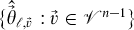
(4) Check if estimates
$\lbrace \hat{\vec{\theta }}_{\ell ,\vec{v}} : \vec{v} \in \mathcal {V}^{n-1}\rbrace$ with ℓ = 0 (1) better represent the SPAM (HAM) training messages than the reverse. If not, keep the correspondence of HAM and SPAM to labels 0 and 1, respectively. Otherwise, flip the correspondence. Since the true labels of the training messages are known partially or not at all, the check utilizes a simple heuristic based on message lengths as discussed in Section 4.3. Note: flipping the correspondence does not have any effect on the training phase, only on the classification phase.





4.2 Gibbs sampling
The initial sample is drawn in a simple way described later. Now, the process of drawing the (m + 1)st sample (1 ≤ m < M) is discussed starting with drawing  $\langle \vec{\theta }_{0,\vec{v}}^{(m+1)}:\vec{v} \in \mathcal {V}^{n-1}\rangle$ from distribution
 \begin{eqnarray*}
Pr\big (\langle \vec{\Theta }_{0,\vec{v}}:\vec{v}\in \mathcal {V}^{n-1}\rangle |\langle \vec{\Theta }_{1,\vec{v}}=\vec{\theta }_{1,\vec{v}}^{(m)}:\vec{v}\in \mathcal {V}^{n-1}\rangle ,\quad \vec{\Phi }=\vec{\phi }^{(m)},\\
\quad C_1 = c_1^{(m)}, \ldots , C_N=c_N^{(m)}, \vec{t},\vec{\gamma },\vec{\delta }\big ).
\end{eqnarray*}
Using Bayes rule, marginalization, generative modeling assumptions, and properties of the Dirichlet distribution, it follows that the probability of  $\langle \vec{\Theta }_{0,\vec{v}}:\vec{v}\in \mathcal {V}^{n-1}\rangle = \langle \vec{\theta }_{0,\vec{v}}^{(m+1)}:\vec{v}\in \mathcal {V}^{n-1}\rangle$ in the above distribution equals
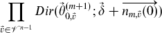 \begin{equation*}
\prod _{\vec{v}\in \mathcal {V}^{n-1}}Dir(\vec{\theta }_{0,\vec{v}}^{(m+1)};\vec{\delta }+\overrightarrow{n_{m,\vec{v}}(0)})
\end{equation*}
where  $\overrightarrow{n_{m,\vec{v}}(0)}$ is the length
 $|\mathcal {V}|$ vector whose kth component equals the number of times the kth token appears immediately to the right of
 $\vec{v}$ in a token sequence, say the ith, whose label during the mth iteration is c (m)i = 0. Due to independence, each
 $\vec{\theta }_{0,\vec{v}}^{(m+1)}$ is drawn from distribution
 \begin{equation*}
Dir(.;\vec{\delta }+\overrightarrow{n_{m,\vec{v}}(0)}).
\end{equation*}
Similar reasoning shows that each  $\vec{\theta }_{1,\vec{v}}^{(m+1)}$ is drawn from distribution
 \begin{equation*}
Dir(.;\vec{\delta }+\overrightarrow{n_{m,\vec{v}}(1)}).
\end{equation*}
Now consider the process of drawing  $\vec{\phi }^{(m+1)}$ from distribution
 \begin{eqnarray*}
Pr\big (\vec{\Phi }|\langle \vec{\Theta }_{0,\vec{v}}=\vec{\theta }_{0,\vec{v}}^{(m+1)}:\vec{v}\in \mathcal {V}^{n-1}\rangle ,\langle \vec{\Theta }_{1,\vec{v}}=\vec{\theta }_{1,\vec{v}}^{(m+1)}:\vec{v}\in \mathcal {V}^{n-1}\rangle ,\\
\quad C_1 = c_1^{(m)}, \ldots , C_N=c_N^{(m)},\vec{t},\vec{\gamma },\vec{\delta }\big ).
\end{eqnarray*}
It can be shown that  $\vec{\phi }^{(m+1)}$ is drawn from distribution
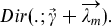
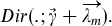 \begin{equation*}
Dir(.;\vec{\gamma }+\overrightarrow{\lambda _m}).
\end{equation*}
where  $\overrightarrow{\lambda _m}$ is the length two vector whose ℓth component (ℓ ∈ {0, 1}) is the number of times the label ℓ appeared among c (m)1, . . . c (m)N.
Finally, given 1 ≤ i ≤ N, consider the process of drawing c (m + 1)i from distribution
 \begin{eqnarray*}
Pr(C_{i}|\langle \vec{\Theta }_{0,\vec{v}} = \vec{\theta }_{0,\vec{v}}^{(m+1)}:\vec{v}\in \mathcal {V}^{n-1}\rangle ,\langle \vec{\Theta }_{1,\vec{v}}=\vec{\theta }_{1,\vec{v}}^{(m+1)}:\vec{v}\in \mathcal {V}^{n-1}\rangle ,\vec{\Phi }=\vec{\phi }^{(m+1)}, \\
C_1 = c_1^{(m+1)}, \ldots , C_{i-1}=c_{i-1}^{(m+1)}, C_{i+1}=c_{i+1}^{(m)}, \ldots , C_N=c_N^{(m)}, \vec{t},\vec{\gamma },\vec{\delta }).
\end{eqnarray*}
Given  $1 \le k \le |\mathcal {V}|$ and
 $\vec{v} \in \mathcal {V}^{n-1}$, let
 $d_{i,\vec{v}}(k)$ denote the number of times the kth token in
 $\mathcal {V}$ appears in the ith message immediately to the right of n − 1 tokens
 $\vec{v}$. Using Bayes rule, marginalization, generative modeling assumptions, and properties of the Dirichlet distribution, it follows that the probability of 0 in the above distribution equals
 \begin{equation}
\frac{\vec{\phi }^{(m+1)}(0)\prod _{\vec{v}\in \mathcal {V}^{n-1}}\prod _{k=1}^{|\mathcal {V}|}\vec{\theta }_{0,\vec{v}}^{(m+1)}(k)^{d_{i,\vec{v}}(k)}}{\mbox{Numerator}+ \vec{\phi }^{(m+1)}(1)\prod _{\vec{v}\in \mathcal {V}^{n-1}}\prod _{k=1}^{|\mathcal {V}|}\vec{\theta }_{1,\vec{v}}^{(m+1)}(k)^{d_{i,\vec{v}}(k)}}.
\end{equation}
If the true label, ci, of the ith message is known during the training phase, then c (m + 1)i is simply set to ci. Otherwise, c (m + 1)i is drawn from {0, 1} with zero probability equal to (1). One way to do so is to employ the following two-step procedure. (i) Generate u uniformly from (0, 1). (ii) If u is less than or equal to (1), then set c (m + 1)i = 0, else set c (m + 1)i = 1. To avoid underflow, the comparison in step (ii) is transformed to an equivalent one in log-space. Namely,
 \begin{equation}
\ \ \ \log _2\left(\frac{\vec{\phi }^{(m+1)}(1)}{\vec{\phi }^{(m+1)}(0)}\right) + \log _2\left(\frac{u}{1-u}\right)+ \sum _{\vec{v}\in \mathcal {V}^{n-1}}\sum _{k=1}^{|\mathcal {V}|}d_{i,\vec{v}}(k)\left[\log _2\left(\frac{\vec{\theta }_{1,\vec{v}}^{(m+1)}(k)}{\vec{\theta }_{0,\vec{v}}^{(m+1)}(k)}\right)\right] \le 0.
\end{equation}
The whole sampling procedure is summarized as follows.
(1) Fix M,
$\vec{\delta }$, and $\vec{\gamma }$.(2) Draw the initial sample.
(a) For each
$\vec{v} \in \mathcal {V}^{n-1}$, draw $\vec{\theta }_{0,\vec{v}}^{(1)}$ and $\vec{\theta }_{1,\vec{v}}^{(1)}$ from $Dir(.;\vec{\delta })$.(b) Draw
$\vec{\phi }^{(1)}$ from $Dir(.;\vec{\gamma })$.(c) For each 1 ≤ i ≤ N, if the true label, ci, of the ith message is known during the training phase, then set c (1)i = ci. Otherwise, draw c (1)i from {0, 1} with zero probability equal to one half.
(3) Draw the (m + 1)st sample, 1 ≤ m < M.
(a) For each
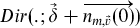
$\vec{v} \in \mathcal {V}^{n-1}$, draw $\vec{\theta }_{0,\vec{v}}^{(m+1)}$ and $\vec{\theta }_{1,\vec{v}}^{(m+1)}$ from $Dir(.;\vec{\delta }+\overrightarrow{n_{m,\vec{v}}(0)})$ and $Dir(.;\vec{\delta }+\overrightarrow{n_{m,\vec{v}}(1)}).$(b) Draw
$\vec{\phi }^{(m+1)}$ from $Dir(.;\vec{\gamma }+\overrightarrow{\lambda _m}).$(c) For each 1 ≤ i ≤ N, if the true label, ci, of the ith message is known during the training phase, then set c (m + 1)i = ci. Otherwise, draw c (m + 1)i from {0, 1} with zero probability equal to (1). This is done as follows.
(i) Draw u uniformly from (0, 1).
(ii) If inequality (2) holds, then set c (m + 1)i = 0, else set c (m + 1)i = 1.




4.3 Checking the HAM (SPAM) correspondence to labels 0 (1)
Here we describe a heuristic for checking if 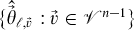 $\lbrace \hat{\vec{\theta }}_{\ell ,\vec{v}}:\vec{v} \in \mathcal {V}^{n-1}\rbrace$ with ℓ = 0 (1) better represents the SPAM (HAM) training messages than the reverse. The heuristic is based on our observation that SPAM messages tend to be longer and have less variance in length than HAM messages. Each training message is assigned a label ℓ. Each message whose true label is available is naturally assigned that label, otherwise, the assignment is made using the procedure described in Section 5. Three quantities are computed from the set of training messages assigned label 0: Mean(0), the mean message length (number of characters); Median(0), the median message length; Variance(0), the message length variance. Likewise, Mean(1), Median(1), Variance(1) are computed from the set of training messages assigned label 1. If at least two of the following conditions are true, then the correspondence of HAM (SPAM) to labels 0 (1) is flipped, otherwise, the correspondence is kept: (i) Mean(0) > Mean(1), (ii) Median(0) > Median(1), (iii) Variance(0) < Variance(1).
5 Classification phase
Let  $\vec{\mu }$ be a length L token sequence for a new message. Let μk denote the kth token and for k ≥ n, let
 $\vec{v}_k$ denote the n − 1 tokens immediately to the left of μk. Let C be a random variable denoting the label of the new message. The message is assigned label 1 if and only if the ratio of its posterior label 1 probability and posterior label 0 probability is greater than one. Using Bayes rule and model independences, this ratio can be simplified as follows.
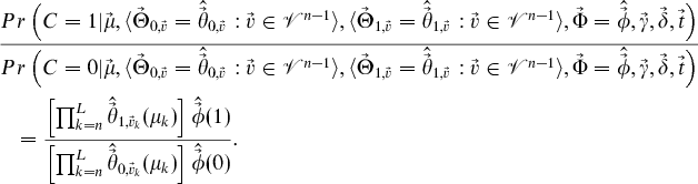 \begin{eqnarray*}
\frac{Pr\left(C=1|\vec{\mu }, \langle \vec{\Theta }_{0,\vec{v}} = \hat{\vec{\theta }}_{0,\vec{v}}:\vec{v}\in \mathcal {V}^{n-1}\rangle , \langle \vec{\Theta }_{1,\vec{v}} = \hat{\vec{\theta }}_{1,\vec{v}}:\vec{v}\in \mathcal {V}^{n-1}\rangle , \vec{\Phi } = \hat{\vec{\phi }}, \vec{\gamma }, \vec{\delta }, \vec{t}\right)}{Pr\left(C=0|\vec{\mu }, \langle \vec{\Theta }_{0,\vec{v}} = \hat{\vec{\theta }}_{0,\vec{v}}:\vec{v}\in \mathcal {V}^{n-1}\rangle , \langle \vec{\Theta }_{1,\vec{v}} = \hat{\vec{\theta }}_{1,\vec{v}}:\vec{v}\in \mathcal {V}^{n-1}\rangle , \vec{\Phi } = \hat{\vec{\phi }}, \vec{\gamma }, \vec{\delta }, \vec{t}\right)} \\
\quad = \frac{\left[\prod _{k=n}^{L}\hat{\vec{\theta }}_{1,\vec{v}_k}(\mu _k) \right]\hat{\vec{\phi }}(1)}{\left[\prod _{k=n}^{L}\hat{\vec{\theta }}_{0,\vec{v}_k}(\mu _k) \right]\hat{\vec{\phi }}(0)}.
\end{eqnarray*}
To avoid underflow, logarithms are taken resulting in the assignment rule: assign label 1 to the new message if and only if
 \begin{equation*}
\sum _{k=n}^L\log _2(\hat{\vec{\theta }}_{1,\vec{v}_k}(\mu _k)) + \log _2(\hat{\vec{\phi }}(1)) - \sum _{k=n}^L\log _2(\hat{\vec{\theta }}_{0,\vec{v}_k}(\mu _k)) - \log _2(\hat{\vec{\phi }}(0)) > 0.
\end{equation*}
The message is classified as SPAM if and only if the message is assigned label ℓ and Step 4 in the overall algorithm in Section 4 produces a correspondence of SPAM to ℓ.
Comment: The log of the posterior ratio above can be used to compute the label 1 posterior probability directly, which can be valuable as a classification confidence value (though, the experiments reported next do not make use of this classification confidence value).
 \begin{eqnarray*}
Pr\left(C=1|\vec{\mu }, \langle \vec{\Theta }_{0,\vec{v}} = \hat{\vec{\theta }}_{0,\vec{v}}:\vec{v}\in \mathcal {V}^{n-1}\rangle , \langle \vec{\Theta }_{1,\vec{v}} = \hat{\vec{\theta }}_{1,\vec{v}}:\vec{v}\in \mathcal {V}^{n-1}\rangle , \vec{\Phi } = \hat{\vec{\phi }}, \vec{\gamma }, \vec{\delta }, \vec{t}\right)\\
\quad = \mbox{Sigmoid}_{2}\left(\sum _{k=n}^L\log _2(\hat{\vec{\theta }}_{1,\vec{v}_k}(\mu _k)) + \log _2(\hat{\vec{\phi }}(1)) - \sum _{k=n}^L\log _2(\hat{\vec{\theta }}_{0,\vec{v}_k}(\mu _k)) - \log _2(\hat{\vec{\phi }}(0)) \right)
\end{eqnarray*}
Sigmoid2(.) denotes the function  $z \in \mathbb {R} \mapsto [1+2^{-z} ]^{-1}$.
6 Experimental setup
6.1 Data
We used a publicly available SMS corpus collected from the UK consisting of 10855 HAM and 1353 SPAM messages. We randomly split the corpus into training (275 SPAM and 7025 HAM messages) and testing (1078 SPAM and 3830 HAM) sets.
The HAM messages were gathered from volunteers in the UK between 2004 and 2007 by Caroline Tagg at the University of Birmingham Tagg (Reference Tagg2009). She made these messages anonymous by replacing certain information (such as names, phone numbers and addresses) with generic strings e.g. NAME12. Upon our request, she made the anonymized messages available to us free of charge. The SPAM messages were gathered by several university researchers who scraped two public on-line forums in the UK between 2003 and 2010. Details regarding the data collection procedure can be found in Section 4.1 of Delany et al. (Reference Delany, Buckley and Greene2012). Upon our request, S. Delany made these SPAM messages available to us free of charge.
Since the HAM messages were anonymized and the SPAM messages were not, the generic anonymization strings (NAME12) could provide classifiers an artificial means for discriminating (e.g. learning that the presence of string NAM is a good HAM indicator). To avoid this problem, we replaced the generic anonymization strings with syntactically meaningful, but arbitrary, strings (e.g. NAME2 by John Doe). The replacements respect the format expected for the generic string category, and we gave each specific string, when repeated across the corpus, the same arbitrary value.
6.2 Classifier implementation details
In all experiments, we set  $\vec{\delta }$ and
 $\vec{\gamma }$ to all ones, B to 250, M to 750, n to two, and
 $\mathcal {V}$ to the following 29 tokens: a, b, . . ., z, ♯, !, and a single space. We mapped each message into a sequence of these tokens: any uppercase letter was mapped to its lowercase equivalent; any digit was mapped to ♯; any whitespace character was mapped to a single space; any other character was mapped to !. In the remainder of the paper, the Bayesian classification method described in Sections 3-5 is referred to as U-Bayes if trained fully unsupervised or S-Bayes if trained semi-supervised.
We implemented the Semi-Boost (Mallapragada et al. Reference Mallapragada, Jin, Jain and Liu2009) semi-supervised learning algorithm to compare against our approach. Unlike our algorithm, each message was not mapped to a sequence of tokens in  $\mathcal {V}$, instead, the characters were used unchanged. The base classifier was an SVM with a linear kernel and the SMO (Sequential Minimal Optimization) algorithm and character bi-grams as features. The message similarity metric used by Semi-Boost was computed as follows.
(i) Each message was mapped to a vector that had an entry for each character bi-gram. Each entry contained the number of times the bi-gram appeared in the message.
(ii) The cosine similarity was computed between their vectors.
Finally, the sampling method used by Semi-Boost was implemented as follows.
(a) The weights for each message were computed using the p and q values in Mallapragada et al. (Reference Mallapragada, Jin, Jain and Liu2009) then normalized to sum to 1.
(b) Each message was added to the sample vector with probability equal to its weight.
(c) The sample vector was sorted decreasing by weight and the top 10 percent of messages were selected as the unlabeled instances to be used in the next boosting iteration.
We also implemented the unsupervised SPAM classification algorithm in Uemura et al. (Reference Uemura, Ikeda, Kida and Arimura2011) but found its accuracy to be low and do not further discuss it. We conjecture the low accuracy to be due to the significantly shorter nature of SMS messages than Email – the genre for which the approach in Uemura et al. (Reference Uemura, Ikeda, Kida and Arimura2011) was designed.
To provide a supervised comparison to our approach, we implemented an SVM with a linear kernel based on the SMO algorithm. The features consisted of all character 3-grams. Note: the SVM used as the base classifier in Semi-Boost used a different set of features (only character 2-grams) than the SVM described here.
6.3 Methodology
Each individual experiment was conducted by first making several choices: (i) choose a pair of classifiers to compare, S-Bayes versus Semi-Boost or U-Bayes versus SVM; (ii) choose train(H) and train(S), the total number of HAM and SPAM training messages to use; (iii) choose train(H,labeled) and train(S,labeled), the number of HAM and SPAM training messages whose labels will be used by S-Bayes, Semi-Boost, and SVM.
Next, the following process was repeated 100 times.
(1) Randomly select, without replacement, train(H) HAM and train(S) SPAM training messages from the corpus. If U-Bayes is among the chosen pair of classifiers, train it ignoring all SPAM and HAM labels. From each of the train(H) HAM and train(S) SPAM message sets, randomly select, without replacement, a subset of train(H,labeled) and train(S,labeled) messages. If Semi-Boost and S-Bayes are among the chosen pair of classifiers, train them on the train(H) and train(S) HAM and SPAM messages ignoring the labels on all but the train(H,labeled) and train(S,labeled) subsets. If SVM is among the chosen pair of classifiers, train it on only the train(H,labeled) and train(S,labeled) subsets (including the labels).
(2) Evaluate the classifiers on the testing message set. For each classifier, record the observed false positive rate and the true positive rate where SPAM is regarded as the positive class.
The results reported for each individual experiment are the average true (false) positive rate TPR (FPR) and 0.95 error bars. The error bar for TPR was computed as follows. At each repetition, the exact binomial test (Langford Reference Langford2006) was employed to compute the 0.95 confidence interval for that repetition. Let {TPR1(+), . . ., TPR100(+)} denote the upper limits on the intervals for the true positive rates over the repetitions and {TPR1(-), . . ., TPR100(-)} denote the lower limits. The upper 0.95 limit on Average{TPR1(+), . . ., TPR100(+)} and lower 0.95 limit on Average{TPR1(-), . . ., TPR100(-)} were both computed by the T-Test. These values form the upper and lower limits for the TPR error bar. An analogous approach is used to compute the FPR error bar.
7 Results
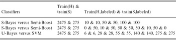
Table 1 describes three series of experiments whose results are discussed in detail in Subsections 7.1 and 7.2. The first two series compared the semi-supervised approaches, S-Bayes and Semi-Boost, as the number of HAM and SPAM labels used in training, train(H,labeled) and train(S,labeled), were varied. The first increased train(H,labeled) + train(S,labeled), while the second increased train(H,labeled)/ train(S,labeled). The third series of experiments compared the unsupervised and fully supervised approaches, U-Bayes and SVM, as the number of labeled training messages used by SVM increased while the number of unlabeled training messages used by U-Bayes remained fixed.
Each row defines a series of experiments.

Since the corpus has a much larger number of HAMs than SPAMs, in all three series, the total number of training HAMs, train(H), was chosen to be much larger (9 times) than the total number of training SPAMs, train(S). To avoid what seemed an excessive imbalance (25 times), train(H) was not chosen to be 7025, the total number of training HAMs available.
7.1 Comparison of semi-supervised approaches
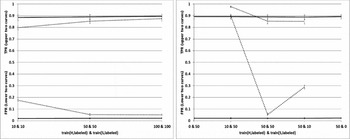
Figure 1 depicts results obtained from the first two series of experiments which compared S-Bayes and Semi-Boost. Two primary observations are in order. (i) S-Bayes clearly outperformed Semi-Boost, especially so when the number of labeled training messages was small. (ii) S-Bayes exhibited more stable behavior than Semi-Boost, particularly so when train(H,labeled)/train(S,labeled) was varied (right chart).
A comparison of S-Bayes (solid curves) and Semi-Boost (dotted curves). In the right chart, no result is shown for Semi-Boost at  $0 \& 50$ and
 $50 \& 0$ since Semi-Boost requires some SPAM and HAM labels.

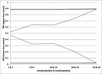
The high-degree of stability of S-Bayes was an unexpected result. We expected that varying the number of HAM and SPAM labels used in training, train(H,labeled) and train(S,labeled), would have affected the TPR or FPR of S-Bayes. However, the TPR and FPR remained essentially constant. To better understand this unexpected behavior, we conducted a series of experiments where S-Bayes was run without any flipping of the correspondence of HAM and SPAM to labels 0 and 1, i.e. step 4 in Subsection 4.1 was dropped. We call this simplified version of S-Bayes, S-Bayes-NoFlipping. Figure 2 depicts the results of a comparison between S-Bayes and S-Bayes-NoFlipping. When the flipping step is dropped the stability disappeared and the expected behavior was observed: TPR and FPR improved sharply as train(H,labeled) + train(S,labeled) increased. Hence, the presence of training labels only seems to affect the correspondence of HAM, SPAM to labels 0, 1 and not the accuracy of the classification of messages to labels 0 and 1. Moreover, the flipping heuristic worked quite well.
A comparison of S-Bayes (solid curves) and S-Bayes-NoFlipping (dotted curves).

7.2 Comparison of unsupervised and fully supervised approaches
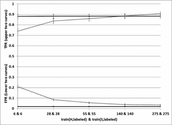
Figure 3 depicts results obtained from the series of experiments which compared U-Bayes and SVM. U-Bayes outperformed SVM when the number of training messages used by SVM was small and performed comparably otherwise. In fact, for the larger numbers of training messages, U-Bayes exhibited a statistically significant FPR advantage over SVM with no statistically significant TPR disadvantage.
A comparison of U-Bayes (solid curves) and SVM (dotted curves).

8 Conclusions
The following conlusions are drawn from the results described in Section 7.
• The Bayesian SPAM classification approach, when used in semi-supervised fashion (S-Bayes), clearly outperformed Semi-Boost.
• The Bayesian SPAM classification approach, when used in fully unsupervised fashion (U-Bayes), outperformed SVM when the number of training messages used by SVM was small and performed comparably otherwise.
• The number of message labels used by S-Bayes in training has little impact on performance. In fact, the TPRs and FPRs observed for U-Bayes were essentially the same as those for S-Bayes over all numbers of labels used.
We believe the Bayesian classification approach (U-Bayes and S-Bayes) works well and is a useful tool for SMS SPAM detection.