1. Introduction
Given that several self-consistent, yet conflicting, models of contact lines (CLs) exist, one can only judge them by comparing their predictions with the experimental data. Such comparisons typically involve the predicted/measured values of the dynamic contact angle (e.g. Le Grand, Daerr & Limat Reference Le Grand, Daerr and Limat2005; Rio et al. Reference Rio, Daerr, Andreotti and Limat2005).
It should be noted, however, that the dynamic contact angle and similar local characteristics (with short-scale variability) are much harder to measure than global parameters, such as, say, the velocity of a drop sliding down an inclined plate. Such a setting, in fact, can be viewed as the simplest testbed for theoretical models of CLs, and it indeed has been used as such by Kim, Lee & Kang (Reference Kim, Lee and Kang2002) and Puthenveettil, Senthilkumar & Hopfinger (Reference Puthenveettil, Senthilkumar and Hopfinger2013) to test a qualitative estimate derived in the former paper. This estimate, however, involves an undetermined constant, hampering the comparison with the experimental data and, thus, suggesting a need for a quantitative theory for drops sliding down an incline.
The first such theory was obtained by Hocking (Reference Hocking1981) for two-dimensional (2D) thin drops described by the lubrication approximation. For the CLs he used the Navier-slip boundary condition and the assumption that the contact angle of an advancing (receding) CL equals
 ${\it\theta}_{a}~({\it\theta}_{r})$
, whereas that of a static CL can assume any value between
 ${\it\theta}_{r}$
and
 ${\it\theta}_{a}$
. In particular, it was shown that sufficiently large drops develop a ‘tail’ of almost uniform thickness. Once the tail has emerged, further increases of the drop’s mass cause only an increase in the length of the tail, whereas the drop’s velocity and amplitude (maximum thickness) remain virtually unchanged. These conclusions have been confirmed by further studies, both numerical and analytical, for various models of CLs (Thiele et al.
Reference Thiele, Neuffer, Bestehorn, Pomeau and Velarde2002; Schwartz, Roux & Cooper-White Reference Schwartz, Roux and Cooper-White2005; Koh et al.
Reference Koh, Lee, Gaskell, Jimack and Thompson2009; Savva & Kalliadasis Reference Savva and Kalliadasis2013).
It should be noted, however, that 2D drops, just like many other two-dimensional liquid structures with CLs, are unstable with respect to transverse perturbations (e.g. Huppert Reference Huppert1982; Silvi & Dussan V. Reference Silvi and Dussan V.1985; Jerrett & de Bruyn Reference Jerrett and de Bruyn1992; Bertozzi & Brenner Reference Bertozzi and Brenner1997; Thiele & Knobloch Reference Thiele and Knobloch2003). As a result, 2D drops are never observed in nature.
Still, they have several important features in common with their 3D counterparts. In particular, sufficiently large 3D drops develop tails too, and an increase of the drop’s mass beyond a certain threshold extends the tail but leaves the drop’s amplitude and velocity unchanged (Podgorski, Flesselles & Limat Reference Podgorski, Flesselles and Limat2001; Le Grand et al. Reference Le Grand, Daerr and Limat2005; Snoeijer et al. Reference Snoeijer, Le Grand-Piteira, Limat, Stone and Eggers2007). Thus, from a technical viewpoint, 2D drops could provide an excellent testing ground for mathematical methods to be later used for 3D drops.
In the present paper, we consider thin drops, both 2D and 3D, sliding down an inclined plate. The 2D case is examined under the sole assumption that the slip length
 $l$
is much smaller than the drop’s size. In the (more difficult) 3D case, we also assume that the Bond number is small and
 ${\it\theta}_{r}={\it\theta}_{a}$
.
The obtained expression for the drop’s velocity is then tested against the experiments of Kim et al. (Reference Kim, Lee and Kang2002). It turns out that the theoretical and experimental results agree only for an unphysically small (subatomic)
 $l$
. Given that our results are derived from the Navier-slip model, one has to conclude that it does not hold for glycerine, glycerine/water mixture and ethylene glycol used in the experiments of Kim et al. (Reference Kim, Lee and Kang2002). Recalling also that the experimental results of Podgorski et al. (Reference Podgorski, Flesselles and Limat2001), Winkels et al. (Reference Winkels, Peters, Evangelista, Riepen, Daerr, Limat and Snoeijer2011) and Puthenveettil et al. (Reference Puthenveettil, Senthilkumar and Hopfinger2013) suggested a subatomic
 $l$
for water and mercury, one might wonder whether the list of exceptions has become long enough to cast doubt on the actual rule.
At the same time, quite paradoxically, the theoretical dependence of the drop’s velocity on the parameters other than
 $l$
does agree with the experimental results, implying that the Navier-slip model can still be used for applications (albeit with an unphysically small
 $l$
). This conclusion agrees with that of Limat (Reference Limat2014), who claimed that, even for water and mercury, the ‘hydrodynamical model describes…logarithmic profiles, correlations between angles…reasonably well, but the price to be paid…seems to be the acceptance of an unphysical cutoff length scale’.
The results outlined above are presented as follows: in § 2 we formulate the problem, in §§ 3 and 4 we examine 2D and 3D drops, and in § 5 we compare our results with those of Kim et al. (Reference Kim, Lee and Kang2002).
2. Formulation of the problem
2.1. The governing equations for 2D drops
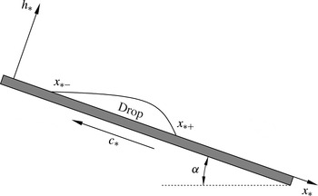
Consider a drop of liquid sliding down a plate inclined at an angle
 ${\it\alpha}$
. The liquid has density
 ${\it\rho}$
, dynamic viscosity
 ${\it\mu}$
and surface tension
 ${\it\sigma}$
, all of which are assumed to be constant in this investigation. We shall first formulate the governing equation for two spatial dimensions, so that the drop’s thickness
 $h_{\ast }$
depends on a single spatial coordinate
 $x_{\ast }$
(with an axis directed down the plate – see figure 1).
The setting (for the two-dimensional case): a drop sliding down an inclined plate.

This paper is concerned with drops steadily sliding with a constant velocity
 $c_{\ast }$
, and it is convenient to assume that the plate is moving in the opposite direction with a matching velocity. In this case, the drop is stationary, and the coordinates
 $x_{\ast \pm }$
of its CLs are time-independent.
Let the drop’s CLs be governed by the Navier-slip boundary condition. We shall also assume that the drop is thin and, thus, can be described by Hocking’s (Reference Hocking1981) lubrication equation. In application to a stationary drop on a moving plate, this equation reduces to
 $$\begin{eqnarray}-c_{\ast }h_{\ast }+\left(\frac{h_{\ast }^{3}}{3}+lh_{\ast }^{2}\right)\left(\frac{{\it\sigma}}{{\it\mu}}\frac{\text{d}^{3}h_{\ast }}{\text{d}x_{\ast }^{3}}+\frac{{\it\rho}g\sin {\it\alpha}}{{\it\mu}}\right)=0,\end{eqnarray}$$
where
 $l$
is the slip length and
 $g$
is the acceleration due to gravity.
We shall first assume that the advancing contact angle equals its receding counterpart, i.e.
 ${\it\theta}_{a}={\it\theta}_{r}={\it\theta}$
, which corresponds to the following boundary conditions:
 $$\begin{eqnarray}h_{\ast }\rightarrow 0,\quad \frac{\text{d}h_{\ast }}{\text{d}x_{\ast }}\rightarrow \mp {\it\theta}\quad \text{as}~x_{\ast }\rightarrow x_{\ast \pm }.\end{eqnarray}$$
Having examined this particular case, we shall briefly discuss how the results obtained can be extended to Hocking’s (Reference Hocking1981) general model
 ${\it\theta}_{r}\neq {\it\theta}_{a}$
(see § 3.4).
Before non-dimensionalising the boundary-value problem (2.1) and (2.2), we note that it does not admit any solutions for the case of perfect wettability. Mathematically, this follows from the fact that, for
 ${\it\theta}=0$
, (2.1) does not have a real solution near the receding CL (see appendix A). Physically, the non-existence of a meaningful solution near
 $x=x_{-}$
reflects the fact that perfectly wetting liquids cannot recede, as they always leave behind a thin layer of liquid. Thus, the case
 ${\it\theta}=0$
will not be examined in this work.
Now, we introduce the following non-dimensional variables:
 $$\begin{eqnarray}x=\frac{x_{\ast }}{X},\quad x_{\pm }=\frac{x_{\ast \pm }}{X},\quad h=\frac{h_{\ast }}{H},\quad c=\frac{c_{\ast }}{C},\end{eqnarray}$$
where
 $$\begin{eqnarray}H=\left(\frac{{\it\sigma}{\it\theta}^{3}}{{\it\rho}g\sin {\it\alpha}}\right)^{1/2},\quad X=\left(\frac{{\it\sigma}{\it\theta}}{{\it\rho}g\sin {\it\alpha}}\right)^{1/2},\quad C=\frac{{\it\sigma}{\it\theta}^{3}}{{\it\mu}}.\end{eqnarray}$$
These particular scales have been chosen to minimise the number of non-dimensional parameters left in the problem. It is also convenient to let
 $$\begin{eqnarray}x_{-}=-XL,\quad x_{+}=0,\end{eqnarray}$$
where
 $L$
is the drop’s non-dimensional length.
By substituting (2.3)–(2.5) into (2.1) and (2.2) and omitting the asterisks, we obtain
 $$\begin{eqnarray}\displaystyle & \displaystyle \frac{\text{d}^{3}h}{\text{d}x^{3}}=-1+\frac{3c}{h(h+3{\it\lambda})}, & \displaystyle\end{eqnarray}$$
 $$\begin{eqnarray}\displaystyle & \displaystyle h=0,\quad \frac{\text{d}h}{\text{d}x}=1\quad \text{at}~x=-L, & \displaystyle\end{eqnarray}$$
 $$\begin{eqnarray}\displaystyle & \displaystyle h=0,\quad \frac{\text{d}h}{\text{d}x}=-1\quad \text{at}~x=0, & \displaystyle\end{eqnarray}$$
 $$\begin{eqnarray}{\it\lambda}=\frac{l}{H}\end{eqnarray}$$
is the non-dimensional slip length. We observe that the third-order equation (2.6) is to be solved with four boundary conditions (2.7) and (2.8). As a result, for given
 ${\it\lambda}$
and
 $L$
, (2.6)–(2.8) determine both
 $h(x)$
and
 $c$
(the latter is, essentially, the problem’s eigenvalue).
Instead of the drop’s length
 $L$
, one can specify (as Hocking (Reference Hocking1981) did) the drop’s cross-sectional area
 $$\begin{eqnarray}\int _{-L}^{0}h\,\text{d}x=A,\end{eqnarray}$$
and treat
 $L$
as an unknown. Such an approach, however, implies mapping the a priori unknown domain
 $(-L,0)$
into a domain with fixed boundaries. It has turned out that solving the problem for a given
 $L$
and then calculating
 $A$
is simpler.
2.2. The governing equations for 3D drops
In the 3D case, the non-dimensional governing equation can be written in the form
 $$\begin{eqnarray}\boldsymbol{{\rm\nabla}}\left[-ch\boldsymbol{e}_{x}+\left(\frac{h^{3}}{3}+{\it\lambda}h^{2}\right)(\boldsymbol{e}_{x}+\boldsymbol{{\rm\nabla}}{\rm\nabla}^{2}h)\right]=0,\end{eqnarray}$$
where
 $\boldsymbol{e}_{x}$
is the unit vector directed along the
 $x$
axis (down the incline), and the
 $y$
axis is implied to be horizontal and perpendicular to the
 $x$
axis. Equation (2.11) can be rewritten in a more convenient form using an auxiliary function
 ${\it\psi}(x,y)$
, such that
 $$\begin{eqnarray}-ch+\frac{h^{3}}{3}\left(1+\frac{\partial {\rm\nabla}^{2}h}{\partial x}\right)=-\frac{\partial {\it\psi}}{\partial y},\quad \frac{h^{3}}{3}\frac{\partial {\rm\nabla}^{2}h}{\partial y}=\frac{\partial {\it\psi}}{\partial x}.\end{eqnarray}$$
These equations are to be solved with the following boundary conditions:
 $$\begin{eqnarray}h=0,\quad {\it\psi}=0\quad \text{at}~\boldsymbol{r}=\boldsymbol{r}_{c},\end{eqnarray}$$
 $$\begin{eqnarray}\boldsymbol{n}\boldsymbol{\cdot }\boldsymbol{{\rm\nabla}}h=1\quad \text{at}~\boldsymbol{r}=\boldsymbol{r}_{c},\end{eqnarray}$$
where
 $\boldsymbol{r}=\boldsymbol{r}_{c}$
is a (parametric or other) representation of the CL and
 $\boldsymbol{n}$
is the inward unit normal to it. It should be noted that the boundary condition for
 ${\it\psi}$
reflects the fact that the mass flux vanishes at the CL. The 3D equivalent of condition (2.10), in turn, is
 $$\begin{eqnarray}\iint _{B}h\,\text{d}x\,\text{d}y=V,\end{eqnarray}$$
where
 $V$
is the drop’s volume and
 $B$
is the drop’s base (i.e. the region bounded by the curve
 $\boldsymbol{r}=\boldsymbol{r}_{c}$
).
2.3. Classification of drops
All results in this paper are based on the assumption that the non-dimensional slip length
 ${\it\lambda}$
is small. Given this, three cases can be distinguished depending on the drop’s non-dimensional horizontal size
 $L$
(and, thus, the Bond number
 $Bo=L^{2}$
):
-
(i) small drops,
 $L\ll 1$
;
-
(ii) medium drops,
${\it\lambda}\ll L\sim 1$
; -
(iii) large drops,
$L\gg 1$
.


We observe that cases 1 and 2 overlap, with the non-overlapping part of the former,
 $L\lesssim {\it\lambda}$
, being of little physical importance (the corresponding drops are too small). Thus, we shall only examine cases 2 and 3.
3. Two-dimensional drops
3.1. The numerical results
Before developing an asymptotic theory for the limit
 ${\it\lambda}\rightarrow 0$
, it is helpful to compute some typical solutions of the boundary-value problem (2.6)–(2.8) and discuss their characteristic features.
The boundary-value problem (2.6)–(2.8) was solved numerically using the algorithm described in appendix B. A wide range of
 ${\it\lambda}$
and
 $L$
was explored.
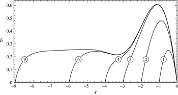
Figure 2 shows examples of drops of increasing lengths. One can see that, by
 $L\approx 5$
, the drop’s front assumes a certain limiting shape which remains the same for all larger drops. One can also observe the ‘tail’ growing behind the frontal part (the same feature was observed by Hocking (Reference Hocking1981), Savva & Kalliadasis (Reference Savva and Kalliadasis2013) and, in a slightly different formulation, by Thiele et al. (Reference Thiele, Neuffer, Bestehorn, Pomeau and Velarde2002)).


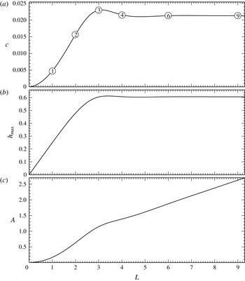
It is instructive to plot the drop’s global characteristics (such as the velocity, maximum thickness and cross-sectional area) as functions of the drop length – see figure 3.
The dependence of a 2D drop’s characteristics on its length
 $L$
(as computed using the boundary-value problem (2.6)–(2.8) with
 ${\it\lambda}=0.001$
): (a) the velocity
 $c$
, (b) the maximum thickness
 $h_{max}$
, (c) the cross-sectional area
 $A$
. The circled numbers in (a) indicate the corresponding values of
 $L$
; the solutions with these values are shown in figure 2.

First, we observe that
 $c$
is small, but not as small as
 ${\it\lambda}$
(except for the smallest drops). In fact, a more precise estimate can be made,
 $$\begin{eqnarray}c=O\left(\frac{1}{\ln {\it\lambda}}\right),\end{eqnarray}$$
which will be confirmed by the asymptotic analysis below.
Second, for
 $L\gtrsim 5$
,
 $c$
and
 $h_{max}$
are effectively constant. This suggests that the length of the tail does not affect the drop’s global characteristics. One can also see that the tail is of virtually uniform thickness (later shown to approximately equal
 $\sqrt{3c}$
), which agrees with the virtually linear dependence of
 $A$
on
 $L$
for
 $L\gtrsim 5$
(see figure 3
c).
The observed features will be used as ‘hints’ when studying the solution’s asymptotic structure. In particular, estimate (3.1) is the basis of all of our asymptotic results, both 2D and 3D.
3.2. Medium drops
The asymptotic structure of 2D medium drops involves an outer region and two boundary layers near the CLs.
The left boundary layer is described by the local variables
 $$\begin{eqnarray}x_{l}=\frac{x+L}{{\it\lambda}},\quad h_{l}=\frac{h}{{\it\lambda}}.\end{eqnarray}$$
In terms of
 $(x_{l},h_{l})$
, (2.6) and the left boundary condition (2.7) become
 $$\begin{eqnarray}\displaystyle & \displaystyle \frac{\text{d}^{3}h_{l}}{\text{d}x_{l}^{3}}=\frac{3c}{h_{l}(h_{l}+3)}+O({\it\lambda}^{2}), & \displaystyle\end{eqnarray}$$
 $$\begin{eqnarray}\displaystyle & \displaystyle h_{l}=0,\quad \frac{\text{d}h_{l}}{\text{d}x_{l}}=1\quad \text{as}~x_{l}\rightarrow 0. & \displaystyle\end{eqnarray}$$
 $c$
, for which (3.3) and (3.4) yield
 $$\begin{eqnarray}\displaystyle h_{l} & = & \displaystyle x_{l}+a^{(1)}x^{2}+c\left[{\textstyle \frac{1}{2}}x_{l}^{2}\ln x_{l}-{\textstyle \frac{1}{2}}(x_{l}+3)^{2}\ln (x_{l}+3)+\left(3\ln 3+{\textstyle \frac{3}{2}}\right)x_{l}+{\textstyle \frac{9}{2}}\ln 3+a^{(2)}x^{2}\right]\nonumber\\ \displaystyle & & \displaystyle +\,O(c^{2}).\end{eqnarray}$$
It turns out that
 $h_{l}$
does not match the outer solution unless
 $a^{(1)}=a^{(2)}=0$
; hence,
 $$\begin{eqnarray}h_{l}=x_{l}+c\left[{\textstyle \frac{1}{2}}x_{l}^{2}\ln x_{l}-{\textstyle \frac{1}{2}}(x_{l}+3)^{2}\ln (x_{l}+3)+\left(3\ln 3+{\textstyle \frac{3}{2}}\right)x_{l}+{\textstyle \frac{9}{2}}\ln 3\right]+O(c^{2}).\end{eqnarray}$$
Next, the outer region is described by the unscaled variables. Accordingly, to match (3.6) to the outer solution, the former is to be expressed in terms of
 $(x,h)$
and re-expanded in
 $c$
,
 $$\begin{eqnarray}h=(x+L)+3c(x+L)[\ln {\it\lambda}-\ln (x+L)+\ln 3]+O(c^{2}).\end{eqnarray}$$
Given estimate (3.1), one can see that the term
 $3c(x+L)\ln {\it\lambda}$
(originating from the first order of the inner solution) is now comparable to the term
 $(x+L)$
(originating from the zeroth order). It can be further shown that higher-order corrections to (3.6) include terms
 $O(c^{n}\ln ^{n}x_{l})$
: if expressed through the outer variables, they contribute to the zeroth order of (3.7) and, thus, should all be taken into account when matching to the outer solution. This property of near-CL boundary layers was first observed by Hocking (Reference Hocking1981), who also suggested a way of handling it (see also Voinov Reference Voinov1976; Lacey Reference Lacey1982; Sibley, Nold & Kalliadasis Reference Sibley, Nold and Kalliadasis2015).
First of all, we observe that, given estimate (3.1), the
 $O({\it\lambda}^{2})$
term in (3.3) is exponentially small and, thus, does not affect any order of our expansion (which is carried out in powers of
 $c$
). Omitting this term, we introduce
 $$\begin{eqnarray}{\it\xi}=c\ln x_{l}.\end{eqnarray}$$
It is also convenient to replace
 $h_{l}$
with
 $$\begin{eqnarray}s=\frac{h_{l}}{x_{l}}.\end{eqnarray}$$
In terms of
 $({\it\xi},s)$
, (3.3) becomes
 $$\begin{eqnarray}-\frac{\text{d}s}{\text{d}{\it\xi}}+c^{2}\frac{\text{d}^{3}s}{\text{d}{\it\xi}^{3}}=\frac{3}{s(s+3\text{e}^{-{\it\xi}/c})}.\end{eqnarray}$$
Keeping in mind that
 $\text{e}^{-{\it\xi}/c}$
is exponentially small, one can readily verify that an asymptotic solution of (3.10) can be written in the form
 $$\begin{eqnarray}s=(-9{\it\xi}+f_{0}+cf_{1})^{1/3}+O(c^{2}),\end{eqnarray}$$
where
 $f_{0}$
and
 $f_{1}$
are constants of integration. Changing
 $({\it\xi},s)$
back to
 $(x_{l},h_{l})$
, we obtain
 $$\begin{eqnarray}h_{l}=x_{l}(-9c\ln x_{l}+f_{0}+cf_{1})^{1/3}+O(c^{2}).\end{eqnarray}$$
Re-expanding (3.12) in
 $c$
and matching the result to the large-
 $x_{l}$
limit of (3.6), we obtain
 $$\begin{eqnarray}f_{0}=1,\quad f_{1}=9\ln 3.\end{eqnarray}$$
Finally, we use (3.2) to express solution (3.12)–(3.13) in terms of the unscaled variables, and then re-expand in
 $c$
(with (3.1) kept in mind), which yields
 $$\begin{eqnarray}h=(x+L)\left\{\left(1-9c\ln \frac{1}{{\it\lambda}}\right)^{1/3}+\frac{3c[-\ln (x+L)+\ln 3]}{\left(1-9c\ln {\displaystyle \frac{1}{{\it\lambda}}}\right)^{2/3}}\right\}+O(c^{2}).\end{eqnarray}$$
This asymptotics will play the role of a boundary condition for the outer solution, and a similar condition can be derived for the right boundary layer,
 $$\begin{eqnarray}h=-x\left\{\left(1+9c\ln {\displaystyle \frac{1}{{\it\lambda}}}\right)^{1/3}-\frac{3c[-\ln (-x)+\ln 3]}{\left(1+9c\ln {\displaystyle \frac{1}{{\it\lambda}}}\right)^{2/3}}\right\}+O(c^{2}).\end{eqnarray}$$
To understand the physical meaning of the asymptotics (3.14) and (3.15), rewrite, say, the latter for
 $\text{d}h/\text{d}x$
,
 $$\begin{eqnarray}\frac{\text{d}h}{\text{d}x}=-\left(1+9c\ln {\displaystyle \frac{1}{{\it\lambda}}}\right)^{1/3}-\frac{3c[-\ln (-x)+\ln 3+1]}{\left(1+9c\ln {\displaystyle \frac{1}{{\it\lambda}}}\right)^{2/3}}+O(c^{2}).\end{eqnarray}$$
This condition can be interpreted as a double-accuracy version of the Voinov–Hocking–Cox law (Voinov Reference Voinov1976; Hocking Reference Hocking1981; Hocking & Rivers Reference Hocking and Rivers1982; Cox Reference Cox1986) applied to the drop’s front CL. The standard leading-order Hocking law corresponds to omitting the
 $O(c)$
term on the right-hand side of (3.16).
Before solving the outer problem, it is convenient to introduce
 $$\begin{eqnarray}{\it\varepsilon}=\frac{1}{9\ln {\displaystyle \frac{1}{{\it\lambda}}}},\end{eqnarray}$$
and rewrite (3.14) and (3.15) in the form
 $$\begin{eqnarray}\displaystyle & \displaystyle h\sim (x+L)\left\{\left(1-\frac{c}{{\it\varepsilon}}\right)^{1/3}+\frac{3c[-\ln (x+L)+\ln 3]}{\left(1-{\displaystyle \frac{c}{{\it\varepsilon}}}\right)^{2/3}}\right\}+O({\it\varepsilon}^{2})\quad \text{as}~x\rightarrow -L, & \displaystyle\end{eqnarray}$$
 $$\begin{eqnarray}\displaystyle & \displaystyle h\sim -x\left\{\left(1+{\displaystyle \frac{c}{{\it\varepsilon}}}\right)^{1/3}-\frac{3c[-\ln (-x)+\ln 3]}{\left(1+{\displaystyle \frac{c}{{\it\varepsilon}}}\right)^{2/3}}\right\}+O({\it\varepsilon}^{2})\quad \text{as}~x\rightarrow 0. & \displaystyle\end{eqnarray}$$
 $$\begin{eqnarray}\displaystyle & h=h^{(0)}+{\it\varepsilon}h^{(1)}+O({\it\varepsilon}^{2}), & \displaystyle\end{eqnarray}$$
 $$\begin{eqnarray}\displaystyle & c={\it\varepsilon}[c^{(0)}+{\it\varepsilon}c^{(1)}+O({\it\varepsilon}^{2})]. & \displaystyle\end{eqnarray}$$
 $$\begin{eqnarray}h^{(0)}=-{\textstyle \frac{1}{6}}(x+M)(x+L)x,\end{eqnarray}$$
where
 $$\begin{eqnarray}M=\frac{6(1+c^{(0)})^{1/3}}{L}\end{eqnarray}$$
and the drop’s leading-order velocity
 $c^{(0)}$
is related to its length
 $L$
by
 $$\begin{eqnarray}(1+c^{(0)})^{1/3}-(1-c^{(0)})^{1/3}={\textstyle \frac{1}{6}}L^{2}.\end{eqnarray}$$
It turns out, however, that for
 ${\it\lambda}\geqslant 10^{-4}$
, the leading-order results are not accurate enough, so we shall calculate
 $c^{(1)}$
.
In the next-to-leading order, (2.6) and the asymptotic boundary conditions (3.18) and (3.19) yield
 $$\begin{eqnarray}\displaystyle & \displaystyle \frac{\text{d}^{3}h^{(1)}}{\text{d}x^{3}}=\frac{3}{h^{(0)2}}, & \displaystyle\end{eqnarray}$$
 $$\begin{eqnarray}\displaystyle & \displaystyle h^{(1)}\sim (x+L)\frac{-c^{(1)}+9c^{(0)}[-\ln (x+L)+\ln 3]}{3(1-c^{(0)})^{2/3}}\quad \text{as}~x\rightarrow -L, & \displaystyle\end{eqnarray}$$
 $$\begin{eqnarray}\displaystyle & \displaystyle h^{(1)}\sim -x\frac{c^{(1)}-9c^{(0)}[-\ln (-x)+\ln 3]}{3(1+c^{(0)})^{2/3}}\quad \text{as}~x\rightarrow 0. & \displaystyle\end{eqnarray}$$
 $h^{(0)}$
into (3.25), it can be rewritten in terms of partial fractions,
 $$\begin{eqnarray}\frac{\text{d}^{3}h^{(1)}}{\text{d}x^{3}}=\frac{A_{1}}{x}+\frac{B_{1}}{x^{2}}+\frac{A_{2}}{x+L}+\frac{B_{2}}{(x+L)^{2}}+\frac{A_{3}}{x+M}+\frac{B_{3}}{(x+M)^{2}},\end{eqnarray}$$
where
 $$\begin{eqnarray}A_{1}=-\frac{216c^{(0)}(L+M)}{L^{3}M^{3}},\quad A_{2}=\frac{216c^{(0)}(M-2L)}{L^{3}(M-L)^{3}},\quad A_{3}=\frac{216c^{(0)}(2M-L)}{M^{3}(M-L)^{3}},\end{eqnarray}$$
 $$\begin{eqnarray}B_{1}=\frac{108c^{(0)}}{L^{2}M^{2}},\quad B_{2}=\frac{108c^{(0)}}{L^{2}(M-L)^{2}},\quad B_{3}=\frac{108c^{(0)}}{M^{2}(M-L)^{2}}.\end{eqnarray}$$
By integrating (3.28) three times and matching the resulting solution to the asymptotics (3.26) and (3.27), we obtain, after some straightforward algebra,
 $$\begin{eqnarray}\displaystyle & & \displaystyle \frac{c^{(1)}}{3}\left[\frac{1}{(1-c^{(0)})^{2/3}}+\frac{1}{(1+c^{(0)})^{2/3}}\right]\nonumber\\ \displaystyle & & \displaystyle =3(\ln 3-1)c^{(0)}\left[\frac{1}{(1-c^{(0)})^{2/3}}+\frac{1}{(1+c^{(0)})^{2/3}}\right]+2(B_{1}+B_{2}+B_{3})-(B_{1}+B_{2})\ln L\nonumber\\ \displaystyle & & \displaystyle \quad -\,\frac{A_{3}M(M-L)-B_{3}(2M-L)}{L}\ln \left(1-\frac{L}{M}\right)+\frac{(A_{1}-A_{2})L-A_{3}(2M-L)}{2}.\end{eqnarray}$$
This equality relates the first-order velocity
 $c^{(1)}$
to the drop length
 $L$
(we recall that
 $M$
,
 $c^{(0)}$
,
 $A_{1,2,3}$
and
 $B_{1,2,3}$
are related to
 $L$
by (3.23)–(3.24) and (3.29)–(3.30)).
The physical meaning of the asymptotic results obtained for medium drops will be discussed in § 3.4, after large drops have also been examined.
3.3. Large drops
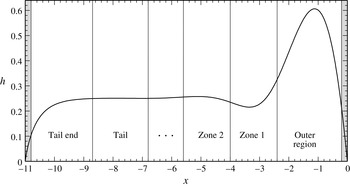
The case of large drops is more complicated than its medium-drop counterpart, mostly due to the fact that it formally involves an infinite sequence of asymptotic zones. This feature was observed for the first time in a problem examined by Wilson & Jones (Reference Wilson and Jones1983), and it has come up four times since then (Bowles Reference Bowles1995; Duchemin, Lister & Lange Reference Duchemin, Lister and Lange2005; Benilov, Benilov & Kopteva Reference Benilov, Benilov and Kopteva2008; Benilov et al. Reference Benilov, Chapman, Mcleod, Ockendon and Zubkov2010). In all four cases, the infinite sequence of zones corresponds physically to a packet of short-scale ripples generated by gravity and surface tension. However, only one or two of the ripples (asymptotic zones) are typically visible in the exact solution, with the other zones being more of a mathematical abstraction. The present case is not an exception to this rule, as illustrated in figure 4.
An illustration (for
 ${\it\lambda}=0.001$
,
 $L=11$
) of the asymptotic structure of the large-drop solution. Observe the small local maximum in Zone 2. The ellipsis ‘
 $\dots$
’ symbolises a (formally infinite) sequence of asymptotic zones representing alternating minima and maxima. The shaded regions are the left and right boundary layers.

Due to the similarity of (2.6) to the case examined by Benilov et al. (Reference Benilov, Benilov and Kopteva2008), we shall consider only the first two zones of the sequence: the outer region (describing the crest of a ripple) and Zone 1 (describing a trough). The rest of the sequence comprises alternating crests and troughs with decreasing amplitudes and widths, rapidly converging to a uniform ‘tail’ (see figure 4). These asymptotic zones will be examined in § 3.3.1, with the remaining two (the ‘tail end’ and the left boundary layer) examined in § 3.3.2.
3.3.1. The drop’s front
It turns out that the velocity of a large drop is determined by the structure of the drop’s rear. This makes the drop’s front less important, so we shall calculate its shape with leading-order accuracy only.
The outer region is described by the ‘natural’ (non-scaled) variables
 $(x,h)$
. Given that we still expect
 $c$
to be small, the original (2.6) in this case reduces, to leading order, to
 $$\begin{eqnarray}\frac{\text{d}^{3}h}{\text{d}x^{3}}=-1.\end{eqnarray}$$
As in the case of a medium drop, the outer region can be matched to the right boundary layer only if we require
 $$\begin{eqnarray}h=0\quad \text{at}~x=0.\end{eqnarray}$$
The left boundary condition, however, cannot be enforced for the outer region (since
 $L\gg 1$
, the left boundary is too far away). It turns out that the outer solution can be matched to the neighbouring zone to its left only if
 $h(x)$
approaches the
 $x$
-axis at a zero angle, which corresponds to the following solution of (3.32) and (3.33):
 $$\begin{eqnarray}h=-{\textstyle \frac{1}{6}}(x+W)^{2}x,\end{eqnarray}$$
where
 $W$
is the width of the drop’s ‘main body’, and it also determines the amplitude of the drop,
 $$\begin{eqnarray}h_{max}={\textstyle \frac{2}{81}}W^{3}.\end{eqnarray}$$
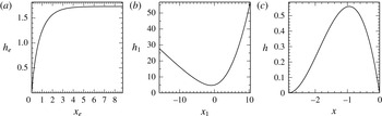
Solution (3.34) is illustrated in figure 5(c).
The solutions (for
 ${\it\lambda}=0.001$
) in the ‘tail end’ (a), in Zone 1 (b) and in the outer region (c).

The right boundary layer should be handled in the same way as it was in the medium-drop case, which yields, at leading order,
 $$\begin{eqnarray}\frac{1}{6}W^{2}=\left(1+9c\ln \frac{1}{{\it\lambda}}\right)^{1/3}.\end{eqnarray}$$
Given relationship (3.35) between
 $h_{max}$
and
 $W$
, this equality relates the (large) drop’s amplitude to its velocity.
Zone 1 is described by the local variables
 $(x_{1},h_{1})$
, such that
 $$\begin{eqnarray}x=-W+c^{1/3}x_{1},\quad h=c^{2/3}h_{1},\end{eqnarray}$$
for which (2.6), to leading order, becomes
 $$\begin{eqnarray}\frac{\text{d}^{3}h_{1}}{\text{d}x_{1}^{3}}=\frac{3}{h_{1}^{2}}.\end{eqnarray}$$
Taking the limit
 $x\rightarrow -W$
of the outer solution (3.34), one can deduce that (3.34) matches
 $h_{1}(x_{1})$
only if
 $$\begin{eqnarray}h_{1}\sim {\textstyle \frac{1}{6}}Wx_{1}^{2}\quad \text{as}~x_{1}\rightarrow \infty .\end{eqnarray}$$
Next, it can be verified that
 $h_{1}(x_{1})$
matches the solution in Zone 2 only if it has the following asymptotic behaviour:
 $$\begin{eqnarray}h_{1}\sim -x_{1}(9\ln x_{1})^{1/3}\quad \text{as}~x_{1}\rightarrow -\infty .\end{eqnarray}$$
The solution of the eigenvalue problem (3.38)–(3.40) was computed numerically (see figure 5 b). As mentioned before, it describes a dip in the drop’s surface, and is flanked by two peaks: the outer region on the right and a much smaller peak on the left (in figure 4, the latter is labelled ‘Zone 2’).
Finally, the ‘tail’ is described by the following solution of (2.6):
 $$\begin{eqnarray}h=(3c)^{1/2}+O({\it\lambda}).\end{eqnarray}$$
3.3.2. The drop’s rear
The ‘tail end’ (see figure 4) is described by the local variables
 $(x_{e},h_{e})$
,
 $$\begin{eqnarray}x=-L+c^{1/6}x_{e},\quad h=c^{1/2}h_{e}.\end{eqnarray}$$
By rewriting (2.6) in terms of
 $(x_{e},h_{e})$
and keeping the leading order only, we obtain
 $$\begin{eqnarray}\frac{\text{d}^{3}h_{e}}{\text{d}x_{e}^{3}}=-1+\frac{3}{h_{e}^{2}}.\end{eqnarray}$$
To match
 $h_{e}(x_{e})$
to the tail solution (3.41), we require
 $$\begin{eqnarray}h_{e}\rightarrow 3^{1/2}\quad \text{as}~x_{e}\rightarrow \infty .\end{eqnarray}$$
It turns out that
 $h_{e}(x_{e})$
matches the left boundary layer (to be examined below) only if
 $$\begin{eqnarray}h_{e}\rightarrow 0\quad \text{as}~x_{e}\rightarrow 0.\end{eqnarray}$$
The solution of problem (3.43)–(3.45) was computed numerically (see § C.2), and it is shown in figure 5(a).
It should be noted also that, as demonstrated in § C.1,
 $h_{e}$
has the following asymptotics:
 $$\begin{eqnarray}h_{e}=-x_{e}\left\{(9\ln x_{e})^{1/3}+\frac{b}{(9\ln x_{e})^{2/3}}+O\left[\frac{\ln (-\ln x_{e})}{\ln ^{5/3}x_{e}}\right]\right\}\quad \text{as}~x_{e}\rightarrow 0.\end{eqnarray}$$
Within the framework of this asymptotics, the constant
 $b$
remains arbitrary, as it is determined by the global solution of problem (3.43)–(3.45). The method for computing
 $b$
is described in § C.3 and it yields
 $$\begin{eqnarray}b\approx -0.613.\end{eqnarray}$$
The left boundary layer for large drops is exactly the same as its medium-drop counterpart, i.e. is represented by expression (3.6). To match it to the asymptotics (3.46) of the tail end, we use (3.42) and (3.2) to deduce
 $$\begin{eqnarray}x_{e}=\frac{{\it\lambda}x_{l}}{c^{1/6}},\quad h_{e}=\frac{{\it\lambda}h_{l}}{c^{1/2}}.\end{eqnarray}$$
Expressing then (3.46) in terms of
 $(x_{l},h_{l})$
and taking advantage of estimate (3.1), we obtain
 $$\begin{eqnarray}h_{l}\sim -x_{l}(9c\ln {\it\lambda})^{1/3}\left(1-\frac{\ln c}{18\ln {\it\lambda}}+\frac{\ln x_{l}}{3\ln {\it\lambda}}+\frac{b}{9\ln {\it\lambda}}+O\left[\frac{\ln (-\ln {\it\lambda})}{\ln ^{2}{\it\lambda}}\right]\right).\end{eqnarray}$$
We also expand the dependence of
 $c$
on
 ${\it\lambda}$
,
 $$\begin{eqnarray}c=\frac{c_{1}}{\ln {\displaystyle \frac{1}{{\it\lambda}}}}+\frac{c_{2}\ln (-\ln {\it\lambda})+c_{3}}{\ln ^{2}{\displaystyle \frac{1}{{\it\lambda}}}}+O\left[\frac{\ln ^{2}(-\ln {\it\lambda})}{\ln ^{3}{\displaystyle \frac{1}{{\it\lambda}}}}\right],\end{eqnarray}$$
where
 $c_{1}$
,
 $c_{2}$
and
 $c_{3}$
are order-one coefficients. On substituting (3.50) into (3.49) and (3.6), and matching these, we obtain
 $$\begin{eqnarray}c_{1}={\textstyle \frac{1}{9}},\quad c_{2}=-{\textstyle \frac{1}{54}},\quad c_{3}={\textstyle \frac{1}{27}}(b+4\ln 3).\end{eqnarray}$$
Thus, expression (3.50) becomes
 $$\begin{eqnarray}c=\frac{1}{9\ln {\displaystyle \frac{1}{{\it\lambda}}}}+\frac{\ln (-\ln {\it\lambda})}{54\ln ^{2}{\displaystyle \frac{1}{{\it\lambda}}}}+\frac{b+4\ln 3}{27\ln ^{2}{\displaystyle \frac{1}{{\it\lambda}}}}+O\left[\frac{\ln ^{2}(-\ln {\it\lambda})}{\ln ^{3}{\it\lambda}}\right],\end{eqnarray}$$
where it should be recalled that
 $b$
is given by (3.47).
3.4. Discussion
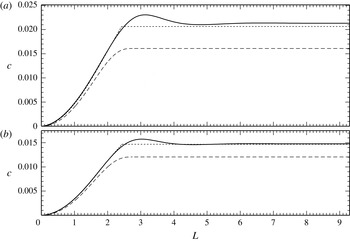
(i) The velocity of medium drops (determined by (3.21), (3.17), (3.24), (3.31)) and that of large drops (given by (3.52)) are compared with the numerical solution of the exact boundary-value problem (2.6)–(2.8) in figure 6. One can see that the numerical and asymptotic results agree reasonably well, especially since the latter are based on expansions in logarithmically small parameters.
The numerical (solid line), zeroth-order asymptotic (dashed line) and first-order asymptotic (dotted line) dependences of the velocity
 $c$
of a 2D drop on its length
 $L$
, for
 ${\it\lambda}=0.001$
, 0.0001. The sloping and horizontal dashed/dotted lines represent the asymptotic results for medium and large drops respectively.

The high accuracy of the results obtained should be attributed to the fact that
 $c$
has been calculated to the first order. The leading-order results, in turn, are not sufficiently accurate for
 ${\it\lambda}\geqslant 10^{-4}$
(see figure 6).
(ii) It is instructive to adapt the medium-drop results to the limit of small Bond number. By assuming
 $L^{2}\ll 1$
in (3.21) and expression (3.24), substituting the resulting
 $c^{(0)}$
and
 $c^{(1)}$
into (3.31), and recalling definition (3.17) of
 ${\it\varepsilon}$
, we obtain
 $$\begin{eqnarray}c=\frac{1}{9\ln {\displaystyle \frac{1}{{\it\lambda}}}}\left[\frac{L^{2}}{4}+O(L^{6})\right]+\frac{1}{81\ln ^{2}{\displaystyle \frac{1}{{\it\lambda}}}}\left[\frac{9}{4}L^{2}\ln \frac{3}{L}+O(L^{4}\ln L)\right]+O\left(\frac{1}{243\ln ^{3}{\displaystyle \frac{1}{{\it\lambda}}}}\right).\end{eqnarray}$$
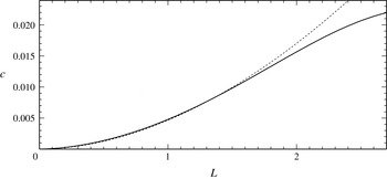
Figure 7 shows that, even though this expression has been formally obtained for small
 $L$
, it is reasonably accurate for
 $L\lesssim 2$
.
The numerical (solid line) and first-order small-Bond-number asymptotic (dotted line) dependences of the velocity
 $c$
of a 2D drop on its length
 $L$
, for
 ${\it\lambda}=0.001$
and medium drops.

(iii) Medium 2D drops have been examined previously by Savva & Kalliadasis (Reference Savva and Kalliadasis2013) using a model similar to our (2.1), but with an extra term describing the hydrostatic pressure gradient (which becomes important in the limit
 ${\it\alpha}\ll 1$
, i.e. if the plate’s slope is small). It can be readily shown that, if
 ${\it\alpha}\sim 1$
, our leading-order medium-drop results agree with those of Savva & Kalliadasis (Reference Savva and Kalliadasis2013).
(iv) We observe that the asymptotic results for medium/large drops (shown by the sloping/horizontal dotted lines in figure 6) do not form a smooth junction. This indicates that there exists an intermediate region where neither approximation works.
This ‘gap’ is a result of the requirement that the parameter
 $M$
in expression (3.22) must exceed the drop length
 $L$
, otherwise the drop thickness becomes negative for some
 $x$
, as does the apparent contact angle at the rear CL. As follows from (3.22) and (3.23), the marginal case
 $M=L$
corresponds to
 $$\begin{eqnarray}L=3^{1/2}2^{2/3}\approx 2.75.\end{eqnarray}$$
Thus, the medium-drop asymptotic results are valid only for
 $L\lesssim 3^{1/2}2^{2/3}$
. The large-drop results, in turn, are valid for
 $L\gg 1$
, which clearly leaves a gap where neither approximation is applicable.
In principle, the gap can be bridged by considering several intermediate limits (starting from
 $L\approx 3^{1/2}2^{2/3}$
). These limits, however, involve a large amount of tedious algebra. Thus, since the results obtained capture the problem’s most important qualitative features (the quadratic nature of
 $c(L)$
for
 $L\ll 1$
and the existence of the limiting velocity for
 $L\gg 1$
), there seems to be little urgency in exploring the intermediate limits.
(v) We recall that the expression for the velocity of large drops is fully determined by matching of the tail end and left boundary layer, i.e. it is not affected by other asymptotic zones. This comes as a surprise, as one would intuitively assume a drop’s velocity to depend on the parameters of the advancing CL or both CLs. This feature indicates the importance of the tail for the dynamics of large drops.
In fact, if one is concerned with the velocity of a large drop and not its shape, one could use (2.6) with the boundary condition describing the left boundary layer,
 $$\begin{eqnarray}h\rightarrow 0,\quad {\displaystyle \frac{\text{d}h}{\text{d}x}}\rightarrow 1\quad \text{as}~x\rightarrow -L,\end{eqnarray}$$
and the tail end,
 $$\begin{eqnarray}h\rightarrow \text{const.}\quad \text{as}~x\rightarrow \infty .\end{eqnarray}$$
For
 $L\gg 1$
, the boundary-value problem (2.6), (3.55) and (3.56) yields
 $c$
which is very close to that of the original problem (2.6)–(2.8). For
 $L\geqslant 6$
(and
 ${\it\lambda}=10^{-3}$
), for example, the two values of
 $c$
differ by less than
 $10^{-5}$
.
(vi) As mentioned before, Hocking (Reference Hocking1981) examined a more general problem, with the boundary conditions (2.2) replaced by
 $$\begin{eqnarray}\displaystyle & \displaystyle h\rightarrow 0,\quad \frac{\text{d}h}{\text{d}x}\rightarrow {\it\theta}_{r}\quad \text{as}\;x\rightarrow x_{-}, & \displaystyle\end{eqnarray}$$
 $$\begin{eqnarray}\displaystyle & \displaystyle h\rightarrow 0,\quad \frac{\text{d}h}{\text{d}x}\rightarrow -{\it\theta}_{a}\quad \text{as}\;x\rightarrow x_{+}. & \displaystyle\end{eqnarray}$$
 ${\it\theta}$
used in the non-dimensionalisation (2.3) and (2.4) be
 ${\it\theta}=({\it\theta}_{r}+{\it\theta}_{a})/2$
, we can write the modified version of the non-dimensional boundary conditions in the form
 $$\begin{eqnarray}h\rightarrow 0=\left\{\begin{array}{@{}ll@{}}{\displaystyle \frac{\text{d}h}{\text{d}x}}\rightarrow {\it\theta}_{-}\quad & \text{as }x\rightarrow -L,\\ {\displaystyle \frac{\text{d}h}{\text{d}x}}\rightarrow -{\it\theta}_{+}\quad & \text{as }x\rightarrow 0,\end{array}\right.\end{eqnarray}$$
where
 $$\begin{eqnarray}{\it\theta}_{-}=\frac{2{\it\theta}_{r}}{{\it\theta}_{r}+{\it\theta}_{a}},\quad {\it\theta}_{+}=\frac{2{\it\theta}_{a}}{{\it\theta}_{r}+{\it\theta}_{a}}.\end{eqnarray}$$
The analysis of the boundary-value problem (2.6), (3.59) is very similar to that in the case
 ${\it\theta}_{r}={\it\theta}_{a}$
, and it will not be presented in detail. We shall only summarise the leading-order results for the drop’s velocity (the next-to-leading-order ones can be obtained in a similar fashion). For a medium drop,
 $c^{(0)}$
satisfies
 $$\begin{eqnarray}({\it\theta}_{-}^{3}+c^{(0)})^{1/3}-({\it\theta}_{+}^{3}-c^{(0)})^{1/3}={\textstyle \frac{1}{6}}L^{2}\end{eqnarray}$$
(compare this equation with (3.24), which implies
 ${\it\theta}_{+}={\it\theta}_{-}=1$
). For large drops, in turn, we have
 $$\begin{eqnarray}c^{(0)}=\frac{{\it\theta}_{-}}{9\ln {\displaystyle \frac{1}{{\it\lambda}}}}.\end{eqnarray}$$
This expression is a generalisation of the first term in expansion (3.52).
4. Three-dimensional drops
The structure of the solution in this case is similar to that of 2D drops: it involves the central (outer) region and a narrow boundary layer near the CL. Since the width of the boundary layer is much smaller than the drop’s size, the boundary layer is essentially two-dimensional. As before, we shall first neglect the hysteresis interval (i.e. assume
 ${\it\theta}_{r}={\it\theta}_{a}$
), with the general case discussed briefly in § 5.2.
Thus, the exact boundary condition (2.14) can be replaced with a 3D equivalent of the asymptotics (3.16) – such that
 $\text{d}h/\text{d}x$
is replaced with
 $-\boldsymbol{n}\boldsymbol{\cdot }\boldsymbol{{\rm\nabla}}h$
and
 $c$
is replaced with the projection of the drop’s velocity onto the normal vector, i.e.
 $c\boldsymbol{n}\boldsymbol{\cdot }\boldsymbol{e}_{x}$
,
 $$\begin{eqnarray}\displaystyle \boldsymbol{n}\boldsymbol{\cdot }\boldsymbol{{\rm\nabla}}h & = & \displaystyle \left(1+9c\boldsymbol{n}\boldsymbol{\cdot }\boldsymbol{e}_{x}\ln {\displaystyle \frac{1}{{\it\lambda}}}\right)^{1/3}\nonumber\\ \displaystyle & & \displaystyle +\,\frac{3c\boldsymbol{n}\boldsymbol{\cdot }\boldsymbol{e}_{x}[-\ln (-x)+\ln 3+1]}{\left(1+9c\boldsymbol{n}\boldsymbol{\cdot }\boldsymbol{e}_{x}\ln {\displaystyle \frac{1}{{\it\lambda}}}\right)^{2/3}}+O(c^{2})\quad \text{at}~\boldsymbol{r}=\boldsymbol{r}_{c}.\end{eqnarray}$$
In what follows, we carry out all calculations to the leading order only, which implies that the terms
 $O(c)$
in (4.1) and the governing equations (2.12) should be omitted. Rewriting the truncated versions of (2.12), (4.1), the boundary conditions (2.13) and the volume condition (2.15) in terms of the polar coordinates
 $(r,{\it\phi})$
, we obtain
 $$\begin{eqnarray}\frac{h^{3}}{3}\left(\cos {\it\phi}+\frac{\partial {\rm\nabla}^{2}h}{\partial r}\right)=-\frac{1}{r}\frac{\partial {\it\psi}}{\partial {\it\phi}},\quad \frac{h^{3}}{3}\left(-\sin {\it\phi}+\frac{1}{r}\frac{\partial {\rm\nabla}^{2}h}{\partial {\it\phi}}\right)=\frac{\partial {\it\psi}}{\partial r},\end{eqnarray}$$
 $$\begin{eqnarray}\frac{{\displaystyle \frac{1}{r}}{\displaystyle \frac{\text{d}R}{\text{d}{\it\phi}}}{\displaystyle \frac{\partial h}{\partial {\it\phi}}}-R{\displaystyle \frac{\partial h}{\partial r}}}{\sqrt{\left({\displaystyle \frac{\text{d}R}{\text{d}{\it\phi}}}\right)^{2}+R^{2}}}=\left[1+3{\hat{c}}\frac{{\displaystyle \frac{\text{d}R}{\text{d}{\it\phi}}}\sin {\it\phi}+R\cos {\it\phi}}{\sqrt{\left({\displaystyle \frac{\text{d}R}{\text{d}{\it\phi}}}\right)^{2}+R^{2}}}\right]^{1/3}\quad \text{at}~r=R({\it\phi}),\end{eqnarray}$$
 $$\begin{eqnarray}h=0,\quad {\it\psi}=0\quad \text{at}~r=R({\it\phi}),\end{eqnarray}$$
 $$\begin{eqnarray}\int _{0}^{\infty }\int _{0}^{2{\rm\pi}}h\,r\,\text{d}r\,\text{d}{\it\phi}=V,\end{eqnarray}$$
where
 $$\begin{eqnarray}{\hat{c}}=3c\ln \frac{1}{{\it\lambda}}\end{eqnarray}$$
and
 $r=R({\it\phi})$
is the polar representation of the CL. The boundary-value problem (4.2)–(4.6) is still not simple enough to be solved analytically. We shall solve (4.2)–(4.6) asymptotically, in the limit of small
 $R$
(or, equivalently, small Bond number).
Since small
 $R$
implies that the drop’s volume
 $V$
is also small, it is convenient to introduce
 $$\begin{eqnarray}{\it\delta}=\left(\frac{4V}{{\rm\pi}}\right)^{1/3}\end{eqnarray}$$
and rescale the variables as follows:
 $$\begin{eqnarray}r_{new}=\frac{r}{{\it\delta}},\quad {\it\phi}_{new}={\it\phi},\end{eqnarray}$$
 $$\begin{eqnarray}h_{new}=\frac{h}{{\it\delta}},\quad {\it\psi}_{new}=\frac{{\it\psi}}{{\it\delta}^{2}},\quad R_{new}=\frac{R}{{\it\delta}},\quad {\hat{c}}_{new}=\frac{{\hat{c}}}{{\it\delta}^{2}}\end{eqnarray}$$
(observe that the scaling of
 ${\hat{c}}$
implies that small drops slide slowly). Substituting (4.8) and (4.9) into (4.2)–(4.5) and omitting the subscript
 $\text{}_{new}$
, we obtain
 $$\begin{eqnarray}\frac{h^{3}}{3}\left({\it\delta}^{2}\cos {\it\phi}+\frac{\partial {\rm\nabla}^{2}h}{\partial r}\right)=-\frac{1}{r}\frac{\partial {\it\psi}}{\partial {\it\phi}},\quad \frac{h^{3}}{3}\left(-{\it\delta}^{2}\sin {\it\phi}+\frac{1}{r}\frac{\partial {\rm\nabla}^{2}h}{\partial {\it\phi}}\right)=\frac{\partial {\it\psi}}{\partial r},\end{eqnarray}$$
 $$\begin{eqnarray}\displaystyle {\displaystyle \frac{1}{R^{2}}}{\displaystyle \frac{\text{d}R}{\text{d}{\it\phi}}}{\displaystyle \frac{\partial h}{\partial {\it\phi}}}-{\displaystyle \frac{\partial h}{\partial r}} & = & \displaystyle \sqrt{1+\left({\displaystyle \frac{1}{R}}{\displaystyle \frac{\text{d}R}{\text{d}{\it\phi}}}\right)^{2}}\nonumber\\ \displaystyle & & \displaystyle +\,{\it\delta}^{2}{\hat{c}}\left({\displaystyle \frac{1}{R}}{\displaystyle \frac{\text{d}R}{\text{d}{\it\phi}}}\sin {\it\phi}+\cos {\it\phi}\right)+O({\it\delta}^{4})\quad \text{at}~r=R({\it\phi}),\end{eqnarray}$$
 $$\begin{eqnarray}h=0,\quad {\it\psi}=0\quad \text{at}~r=R({\it\phi}),\end{eqnarray}$$
 $$\begin{eqnarray}\int _{0}^{2{\rm\pi}}\int _{0}^{R}h\,r\,\text{d}r\,\text{d}{\it\phi}=\frac{{\rm\pi}}{4}.\end{eqnarray}$$
We seek a solution in the form
 $$\begin{eqnarray}h=h^{(0)}+{\it\delta}^{2}h^{(1)}+\cdots \,,\quad {\it\psi}={\it\psi}^{(0)}+{\it\delta}^{2}{\it\psi}^{(1)}+\cdots \,,\end{eqnarray}$$
 $$\begin{eqnarray}R=R^{(0)}+{\it\delta}^{2}R^{(1)}+\cdots \,,\quad {\hat{c}}={\hat{c}}^{(0)}+\cdots \,.\end{eqnarray}$$
Expanding (4.10)–(4.13) to leading order, one can deduce that
 $$\begin{eqnarray}R^{(0)}=1,\quad h^{(0)}={\textstyle \frac{1}{2}}(1-r^{2}),\quad {\it\psi}^{(0)}=0.\end{eqnarray}$$
In the next order, (4.10)–(4.13) yield
 $$\begin{eqnarray}\displaystyle & \displaystyle h^{(0)2}h^{(1)}\frac{\partial {\rm\nabla}^{2}h^{(0)}}{\partial r}+\frac{h^{(0)3}}{3}\left(\cos {\it\phi}+\frac{\partial {\rm\nabla}^{2}h^{(1)}}{\partial r}\right)=-\frac{1}{r}\frac{\partial {\it\psi}^{(1)}}{\partial {\it\phi}}, & \displaystyle\end{eqnarray}$$
 $$\begin{eqnarray}\displaystyle & \displaystyle \frac{h^{(0)3}}{3}\left(-\sin {\it\phi}+\frac{1}{r}\frac{\partial {\rm\nabla}^{2}h^{(1)}}{\partial {\it\phi}}\right)=\frac{\partial {\it\psi}^{(1)}}{\partial r}, & \displaystyle\end{eqnarray}$$
 $$\begin{eqnarray}\displaystyle & -{\displaystyle \frac{\partial h^{(1)}}{\partial r}}-{\displaystyle \frac{\partial ^{2}h^{(0)}}{\partial r^{2}}}R^{(1)}={\hat{c}}^{(0)}\cos {\it\phi}\quad \text{at}~r=1, & \displaystyle\end{eqnarray}$$
 $$\begin{eqnarray}h^{(1)}+{\displaystyle \frac{\partial h^{(0)}}{\partial r}}R^{(1)}=0,\quad {\it\psi}^{(1)}+{\displaystyle \frac{\partial {\it\psi}^{(0)}}{\partial r}}R^{(1)}=0\quad \text{at}~r=1,\end{eqnarray}$$
 $$\begin{eqnarray}\int _{0}^{2{\rm\pi}}\int _{0}^{1}h^{(1)}r\,\text{d}r\,\text{d}{\it\phi}=0.\end{eqnarray}$$
Seeking the solution of these equations in the form
 $$\begin{eqnarray}h^{(1)}(r,{\it\phi})={\hat{h}}^{(1)}(r)\,\cos {\it\phi},\quad {\it\psi}^{(1)}(r,{\it\phi})=\hat{{\it\psi}}^{(1)}(r)\,\sin {\it\phi},\quad R^{(1)}({\it\phi})=\hat{R}^{(1)}\cos {\it\phi},\end{eqnarray}$$
then taking into account expressions (4.24), and eventually eliminating
 $R^{(1)}$
, we obtain
 $$\begin{eqnarray}\displaystyle & \displaystyle \frac{\text{d}}{\text{d}r}\left[\frac{1}{r}\frac{\text{d}}{\text{d}r}\left(r\frac{\text{d}{\hat{h}}^{(1)}}{\text{d}r}\right)-\frac{1}{r^{2}}{\hat{h}}^{(1)}\right]+\frac{24}{r(1-r^{2})^{3}}\hat{{\it\psi}}^{(1)}=-1, & \displaystyle\end{eqnarray}$$
 $$\begin{eqnarray}\displaystyle & \displaystyle \frac{1}{r}\left[\frac{1}{r}\frac{\text{d}}{\text{d}r}\left(r\frac{\text{d}{\hat{h}}^{(1)}}{\text{d}r}\right)-\frac{1}{r^{2}}{\hat{h}}^{(1)}\right]+\frac{24}{(1-r^{2})^{3}}\frac{\text{d}\hat{{\it\psi}}^{(1)}}{\text{d}r}=-1, & \displaystyle\end{eqnarray}$$
 $$\begin{eqnarray}-{\displaystyle \frac{\text{d}{\hat{h}}^{(1)}}{\text{d}r}}+{\hat{h}}^{(1)}={\hat{c}}^{(0)},\quad \hat{{\it\psi}}^{(1)}=0\quad \text{at}~r=1.\end{eqnarray}$$
It is convenient to introduce
 $$\begin{eqnarray}F=\frac{\text{d}^{2}{\hat{h}}^{(1)}}{\text{d}r^{2}}+\frac{1}{r}\frac{\text{d}{\hat{h}}^{(1)}}{\text{d}r}-\frac{1}{r^{2}}{\hat{h}}^{(1)},\end{eqnarray}$$
which allows one to eliminate
 ${\it\psi}^{(1)}$
from (4.23)–(4.25) and decouple
 $F$
from
 ${\hat{c}}^{(0)}$
,
 $$\begin{eqnarray}\displaystyle & \displaystyle r^{2}(1-r^{2})\frac{\text{d}^{2}F}{\text{d}r^{2}}+r(1-7r^{2})\frac{\text{d}F}{\text{d}r}-(1-r^{2})F=7r^{3}-r^{2}-r+1, & \displaystyle\end{eqnarray}$$
 $$\begin{eqnarray}\displaystyle & F\sim \text{const.}\quad \text{as}~r\rightarrow 1, & \displaystyle\end{eqnarray}$$
 $$\begin{eqnarray}\displaystyle & \displaystyle F\sim -1-{\textstyle \frac{1}{2}}r\ln r\quad \text{as}~r\rightarrow 0 & \displaystyle\end{eqnarray}$$
 $$\begin{eqnarray}{\hat{c}}^{(0)}=-\int _{0}^{1}r^{2}F\,\text{d}r.\end{eqnarray}$$
The boundary-value problem (4.27)–(4.29) has been solved numerically (by shooting) and the integral in (4.30) was evaluated to yield
 $$\begin{eqnarray}{\hat{c}}^{(0)}\approx 0.48501.\end{eqnarray}$$
Recalling scaling (4.9) of
 ${\hat{c}}$
, relationship (4.6) of
 ${\hat{c}}$
to the non-dimensional velocity
 $c$
, definition (4.7) of
 ${\it\delta}$
, and non-dimensionalisation (2.3) and (2.4), we obtain for the drop’s dimensional velocity
 $$\begin{eqnarray}c_{\ast }\approx 0.18992\frac{V_{\ast }^{2/3}{\it\theta}^{4/3}{\it\rho}g\sin {\it\alpha}}{{\it\mu}\ln {\displaystyle \frac{X}{l}}},\end{eqnarray}$$
where
 $V_{\ast }$
is the dimensional volume and
 $X$
is defined by (2.4).
Expression (4.32) is the main result of the present paper.
5. Discussion
5.1. Comparison with the results of Kim et al. (Reference Kim, Lee and Kang2002)
Kim et al. (Reference Kim, Lee and Kang2002), hereafter referred to as KLK02, examined the energy balance of drops sliding down an inclined plate and obtained a qualitative estimate for their velocity. As many qualitative estimates do, this one involves an undetermined non-dimensional constant.
In what follows, this constant will be fixed by adapting the estimate of KLK02 to the thin-drop limit and matching the result to our expression (4.32). Once the constant is determined, it can be used in the original estimate for arbitrary drops, turning it into a quantitative formula. This plan is best understood through an analogy with an outer asymptotic solution involving undetermined parameters which can be fixed through matching with the inner solution.
KLK02 obtained the following expression for the dimensional velocity:
 $$\begin{eqnarray}c_{\ast }\approx {\it\gamma}\frac{{\it\rho}g}{{\it\mu}c({\it\theta})\,s({\it\theta})}\frac{V_{\ast }^{2/3}(\sin {\it\alpha}-\sin {\it\alpha}_{c})}{\ln {\displaystyle \frac{R_{b}}{l}}},\end{eqnarray}$$
where
 ${\it\gamma}$
is an undetermined constant,
 $V_{\ast }$
is the drop’s dimensional volume,
 ${\it\alpha}_{c}$
is the critical value of the inclination angle
 ${\it\alpha}$
(such that, for
 ${\it\alpha}<{\it\alpha}_{c}$
, the drop remains static),
 $R_{b}$
is the radius of the drop’s base and
 $$\begin{eqnarray}c({\it\theta})=\frac{2{\it\theta}\sin ^{2}{\it\theta}-\frac{1}{2}\sin 2{\it\theta}+\frac{1}{4}\sin 4{\it\theta}}{(\sin 2{\it\theta}-2{\it\theta})^{2}},\quad s({\it\theta})=\frac{2^{4/3}\sin {\it\theta}}{3^{1/3}(1-\cos {\it\theta}-\frac{1}{2}\cos {\it\theta}\,\sin ^{2}{\it\theta})^{1/3}}.\end{eqnarray}$$
In order to adapt expression (5.1) to the case of thin drops, we observe that
 $$\begin{eqnarray}c({\it\theta})\sim {\textstyle \frac{3}{4}}{\it\theta}^{-1},\quad s({\it\theta})\sim 2^{4/3}3^{-1/3}{\it\theta}^{-1/3}\quad \text{as}~{\it\theta}\rightarrow 0.\end{eqnarray}$$
It should be noted also that, unlike us, KLK02 assumed different values for the advancing and receding contact angles (which is why they have
 ${\it\alpha}_{c}\neq 0$
). The advantages/shortcomings of the two models will be discussed later, whereas here we simply adapt the results of KLK02 to our assumptions, i.e. set
 $$\begin{eqnarray}{\it\alpha}_{c}=0.\end{eqnarray}$$
We also assume that the ratio of
 $R_{b}$
to our spatial scale
 $X$
(defined by (2.4)) is much smaller than the ratio of either of them to the slip length
 $l$
, which implies that
 $$\begin{eqnarray}\ln {\displaystyle \frac{R_{b}}{l}}\approx \ln \frac{X}{l}.\end{eqnarray}$$
Substitution of (5.3)–(5.5) into (5.1) yields
 $$\begin{eqnarray}c_{\ast }\approx \frac{{\it\gamma}}{2^{-2/3}3^{2/3}}\frac{{\it\rho}g\sin {\it\alpha}}{{\it\mu}\ln {\displaystyle \frac{X}{l}}}V_{\ast }^{2/3}{\it\theta}^{4/3}.\end{eqnarray}$$
This expression has exactly the same dependence on the physical parameters as that of our expression (4.32), which should be viewed as an extra validation for both results. Furthermore, comparing (5.6) with (4.32), one can deduce that
 $$\begin{eqnarray}{\it\gamma}\approx 0.24887.\end{eqnarray}$$
With
 ${\it\gamma}$
given by (5.7), formula (5.1) becomes a quantitative result (and it is still valid for thick drops, of course).
It is interesting to compare the theoretical value (5.7) with the experimental ones obtained by KLK02 and Puthenveettil et al. (Reference Puthenveettil, Senthilkumar and Hopfinger2013) (the latter work will be referred to as PSH13). It should be noted that both papers assume
 $$\begin{eqnarray}l\sim 10^{-8}~\text{m}.\end{eqnarray}$$
The values of
 ${\it\gamma}$
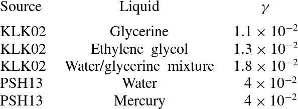
extracted from the results of KLK02 and PSH13 are presented in table 1. We observe that the values obtained for different liquids differ from each other by a factor of up to 3.6, and even the largest one is smaller than the theoretical value (5.7) by a factor of more than 7. In principle, an agreement between the experimental and theoretical results can be achieved by assuming a value of
 $l$
different from (5.8), but, practically, this does not work because
 $l$
becomes unphysically small (subatomic).
The experimental values of the coefficient
 ${\it\gamma}$
from expression (5.1) extracted from the results of KLK02 (Kim et al.
Reference Kim, Lee and Kang2002) and PSH13 (Puthenveettil et al.
Reference Puthenveettil, Senthilkumar and Hopfinger2013), for various liquids.

We conclude that the Navier-slip model of CLs (from which our results have been derived) does not hold for glycerine, glycerine/water mixture or ethylene glycol (used in the experiments of Kim et al.
Reference Kim, Lee and Kang2002). Recalling also that Podgorski et al. (Reference Podgorski, Flesselles and Limat2001), Winkels et al. (Reference Winkels, Peters, Evangelista, Riepen, Daerr, Limat and Snoeijer2011) and Puthenveettil et al. (Reference Puthenveettil, Senthilkumar and Hopfinger2013) observed unphysically small
 $l$
for water and mercury, one cannot help wondering whether the Navier-slip model has sound physical foundations.
At the same time, quite paradoxically, the dependence of our results on the parameters other than
 $l$
does agree with the results of Kim et al. (Reference Kim, Lee and Kang2002). This conclusion agrees with that of Limat (Reference Limat2014), who claimed that the ‘hydrodynamical model describes…logarithmic profiles, correlations between angles…reasonably well, but the price to be paid…seems to be the acceptance of an unphysical cutoff length scale’.
This suggests that, until a physically consistent model of CLs is developed, the Navier-slip model (with an unphysically small
 $l$
) can still be used in, say, industrial applications.
5.2. The effect of the hysteresis interval
It should be noted that our approach (as well as that of all researchers assuming
 ${\it\theta}_{a}={\it\theta}_{r}$
) implies that drops slide for all values of the inclination angle
 ${\it\alpha}$
. Experiments, on the other hand, show that, for most liquid/substrate combinations, there exists a critical value
 ${\it\alpha}_{c}$
such that, if
 ${\it\alpha}<{\it\alpha}_{c}$
, the drop remains static. This is usually attributed to the existence of a hysteresis interval, i.e. a range of contact angles for which the CL remains static.
This seems to imply that our results are valid only if the hysteresis interval is narrow, and, even though such materials do exist (e.g. Glassmaker et al. Reference Glassmaker, Jagota, Hui, Noderer and Chaudhury2007; Smith et al. Reference Smith, Dhiman, Anand, Reza-Garduno, Cohen, McKinleya and Varanasi2013), it is still a restriction.
Models involving hysteresis, however, are associated with a certain difficulty.
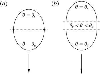
Indeed, even though they work well in two dimensions, for 3D drops they appear to give rise to singularities at the points where the tangent to the CL is parallel to the drop’s velocity (see figure 8
a). At such points, a model with
 ${\it\theta}_{a}\neq {\it\theta}_{r}$
implies a jump in the value of the contact angle.
A 3D drop viewed from above (a schematic). The arrow shows the direction of motion. (a) If all of the CL is curved, two points exist (shown by black dots) where the contact angle changes abruptly from its receding value
 ${\it\theta}_{r}$
to its advancing value
 ${\it\theta}_{a}$
. (b) To resolve the singularity, two straight segments should be introduced to the CL, along which
 ${\it\theta}$
changes continuously from
 ${\it\theta}_{r}$
to
 ${\it\theta}_{a}$
.

A solution to this problem has been suggested by Dussan V. & Chow (Reference Dussan V. and Chow1983), who assumed that the drop’s CL involves straight-line segments (see figure 8
b) along which the contact angle changes continuously from
 ${\it\theta}_{a}$
to
 ${\it\theta}_{r}$
, and such segments have indeed been observed experimentally (Bikerman Reference Bikerman1950; Furmidge Reference Furmidge1962; Rio et al.
Reference Rio, Daerr, Andreotti and Limat2005).
An alternative way to introduce a critical inclination angle consists in letting the plate be inhomogeneous. Following this idea, Savva & Kalliadasis (Reference Savva and Kalliadasis2013) examined 2D drops on an inclined plate with topography and chemical inhomogeneities, and it can be deduced from their results that inhomogeneities can make drops static, for a sufficiently small inclination angle, even if
 ${\it\theta}_{a}={\it\theta}_{r}$
.
6. Concluding remarks
Thus, we have examined two- and three-dimensional drops sliding down an inclined plate, with their sizes exceeding the slip length
 $l$
. Our main result is the asymptotic expression (4.32) for the sliding velocity
 $c_{\ast }$
of a three-dimensional thin and small drop (where ‘small’ means ‘with a small Bond number’).
The expression for
 $c_{\ast }$
has been matched to a qualitative estimate obtained by Kim et al. (Reference Kim, Lee and Kang2002) for arbitrary drops (not necessarily thin and small). The matching fixes the undetermined coefficient involved in this estimate, transforming it into a quantitative result for arbitrary drops.
It turns out, however, that the Navier-slip model of CLs (and, hence, our results) agrees with the available experimental data only for an unphysically small slip length. Still, the dependence on all other parameters does agree with the experiments (under the additional requirement that the drop’s Reynolds number be small). Thus, until a physically consistent model of CLs is developed, our results (as well as the underlying Navier-slip model) can still be used in, say, industrial applications.
Generally, given the large number of alternative models of CLs, it would be very interesting to use them to calculate the velocity of sliding drops and compare the results with those of the experiments. This should enable one to determine the model that is not just useful for applications, but is also relevant physically. One such model could be that of Shikhmurzaev (Reference Shikhmurzaev1993), for which Puthenveettil et al. (Reference Puthenveettil, Senthilkumar and Hopfinger2013) obtained reasonable values for all of the adjustable parameters involved.
Another potential extension of our results consists in introducing a hysteresis interval, i.e. assuming
 ${\it\theta}_{a}>{\it\theta}_{r}$
. If it is sufficiently narrow, and the Bond number is still small, the problem can be treated using an asymptotic approach similar to the one of this work. One can also examine drops on an inhomogeneous substrate: the inhomogeneities (as shown for 2D drops by Savva & Kalliadasis Reference Savva and Kalliadasis2013) would produce a similar effect to hysteresis even if
 ${\it\theta}_{r}={\it\theta}_{a}$
.
Finally, it would be interesting to examine the effect of inertia (by assuming that the drop’s Reynolds number is order one). It should be noted, however, that even though it should change the global parameters of the drop, it is unlikely to affect the local dynamics of the CL (due to the extremely small spatial scale of the processes involved).
Acknowledgements
We acknowledge the support of the Science Foundation Ireland under Grants 11/RFP.1/MTH3281 and 12/IA/1683.
Appendix A. The case of zero contact angle
There seems to exist only one kind of asymptotics of the solution of (2.1) that corresponds to the contact angle being zero. In application to the advancing CL (located at
 $x=0$
), it has the form
 $$\begin{eqnarray}h=B(-x)^{3/2}+D(-x)^{n}+O[(-x)^{3}]\quad \text{as}~x\rightarrow -0,\end{eqnarray}$$
where
 $B$
,
 $C$
and
 $n$
are undetermined constants. It should be noted that the asymptotics (A 1) is self-consistent only if
 $$\begin{eqnarray}{\textstyle \frac{3}{2}}<n<3.\end{eqnarray}$$
On substituting (A 1) into (2.1), we obtain
 $$\begin{eqnarray}\displaystyle & \displaystyle B^{2}=\frac{8{\it\mu}c_{\ast }}{3{\it\sigma}l}, & \displaystyle\end{eqnarray}$$
 $$\begin{eqnarray}\displaystyle & n(n-1)(n-2)-{\textstyle \frac{3}{8}}=0, & \displaystyle\end{eqnarray}$$
 $D$
remains undetermined (it can be determined by matching the local solution (A 1) to the global one). The cubic (A 4) can be readily solved, and one of its roots,
 $$\begin{eqnarray}n={\textstyle \frac{1}{4}}(5+\sqrt{13})\approx 2.15,\end{eqnarray}$$
satisfies condition (A 2).
Next, assume asymptotics similar to (A 1), but for the receding CL, i.e.
 $$\begin{eqnarray}h=B(x+L)^{3/2}+D(x+L)^{n}+O[(x+L)^{3}]\quad \text{as}~x\rightarrow L+0.\end{eqnarray}$$
On substituting this expansion into (2.1), one can verify that
 $n$
again satisfies (A 4), but
 $$\begin{eqnarray}B^{2}=-\frac{8{\it\mu}c_{\ast }}{3{\it\sigma}l}.\end{eqnarray}$$
Thus, no real solutions exist for a receding CL with zero contact angle.
Appendix B. The numerical method for problem (2.6)–(2.8)
When computing the solution of the boundary-value problem (2.6)–(2.8), the main difficulty results from the fact that (2.6) is singular at both boundaries (where the coefficient of the highest derivative vanishes).
To bypass this difficulty, observe that (2.6) admits a Frobenius-style expansion about
 $x=-L$
,
 $$\begin{eqnarray}\displaystyle h & = & \displaystyle P_{1}(x+L)+P_{2}(x+L)^{2}+Q_{2}(x+L)^{2}\ln (x+L)+P_{3}(x+L)^{3}\nonumber\\ \displaystyle & & \displaystyle +\,Q_{3}(x+L)^{3}\ln (x+L)+O[(x+L)^{4}\ln ^{2}(x+L)]\quad \text{as}~x\rightarrow -L+0.\end{eqnarray}$$
On substituting (B 1) into (2.6) and (2.7), one obtains
 $$\begin{eqnarray}\left.\begin{array}{@{}c@{}}P_{1}=1,\quad P_{3}=-\left({\displaystyle \frac{1}{9{\it\lambda}}}+{\displaystyle \frac{Q_{2}}{3}}\right){\displaystyle \frac{c}{2{\it\lambda}}}-{\displaystyle \frac{11c^{2}+12{\it\lambda}^{2}}{72{\it\lambda}^{2}}},\\ Q_{2}={\displaystyle \frac{c}{2{\it\lambda}}},\quad Q_{3}=-{\displaystyle \frac{c^{2}}{12{\it\lambda}^{2}}}.\end{array}\right\}\end{eqnarray}$$
A similar expansion can be derived from (2.6) and the boundary condition (2.8) for the vicinity of
 $x=0$
,
 $$\begin{eqnarray}h=C_{1}x+C_{2}x^{2}+D_{2}x^{2}\ln (-x)+C_{3}x^{3}+D_{3}x^{3}\ln (-x)+O[x^{4}\ln ^{2}(-x)]\quad \text{as}~x\rightarrow -0,\end{eqnarray}$$
where
 $$\begin{eqnarray}\left.\begin{array}{@{}c@{}}C_{1}=-1,\quad C_{3}=-\left({\displaystyle \frac{1}{9{\it\lambda}}}+{\displaystyle \frac{D_{2}}{3}}\right){\displaystyle \frac{c}{2{\it\lambda}}}-{\displaystyle \frac{11c^{2}+12{\it\lambda}^{2}}{72{\it\lambda}^{2}}},\\ D_{2}=-{\displaystyle \frac{c}{2{\it\lambda}}},\quad D_{3}={\displaystyle \frac{c^{2}}{12{\it\lambda}^{2}}}.\end{array}\right\}\end{eqnarray}$$
We observe that the coefficients
 $P_{2}$
and
 $C_{2}$
remain undetermined (they can only be fixed by matching the local expansions (B 1) and (B 3) to the global solution).
Expressions (B 1)–(B 2) and (B 3)–(B 4) can be used to ‘shift’ the boundary conditions away from the singular points
 $x=-L$
and
 $x=0$
to
 $x=-L+{\it\Delta}$
and
 $x=-{\it\Delta}$
(where
 ${\it\Delta}$
is small). Thus, (2.7) and (2.8) are to be replaced with
 $$\begin{eqnarray}\displaystyle (h)_{x=-L+{\it\Delta}} & = & \displaystyle {\it\Delta}+P_{2}{\it\Delta}^{2}+{\displaystyle \frac{c}{2{\it\lambda}}}{\it\Delta}^{2}\ln {\it\Delta}\nonumber\\ \displaystyle & & \displaystyle -\,\left[\left({\displaystyle \frac{1}{9{\it\lambda}}}+{\displaystyle \frac{Q_{2}}{3}}\right){\displaystyle \frac{c}{2{\it\lambda}}}+{\displaystyle \frac{11c^{2}+12{\it\lambda}^{2}}{72{\it\lambda}^{2}}}\right]{\it\Delta}^{3}-{\displaystyle \frac{c^{2}}{12{\it\lambda}^{2}}}{\it\Delta}^{3}\ln {\it\Delta},\end{eqnarray}$$
 $$\begin{eqnarray}\displaystyle \left(\frac{\text{d}h}{\text{d}x}\right)_{x=-L+{\it\Delta}} & = & \displaystyle 1+2P_{2}{\it\Delta}+{\displaystyle \frac{c}{2{\it\lambda}}}{\it\Delta}(2\ln {\it\Delta}+1)\nonumber\\ \displaystyle & & \displaystyle -\,3\left[\left({\displaystyle \frac{1}{9{\it\lambda}}}+{\displaystyle \frac{Q_{2}}{3}}\right){\displaystyle \frac{c}{2{\it\lambda}}}+{\displaystyle \frac{11c^{2}+12{\it\lambda}^{2}}{72{\it\lambda}^{2}}}\right]{\it\Delta}^{2}-{\displaystyle \frac{c^{2}}{12{\it\lambda}^{2}}}{\it\Delta}^{2}(3\ln {\it\Delta}+1),\nonumber\\ \displaystyle & & \displaystyle\end{eqnarray}$$
 $$\begin{eqnarray}\displaystyle (h)_{x=-{\it\Delta}} & = & \displaystyle -{\it\Delta}+C_{2}{\it\Delta}^{2}-{\displaystyle \frac{c}{2{\it\lambda}}}{\it\Delta}^{2}\ln {\it\Delta}\nonumber\\ \displaystyle & & \displaystyle -\,\left[\left({\displaystyle \frac{1}{9{\it\lambda}}}+{\displaystyle \frac{D_{2}}{3}}\right){\displaystyle \frac{c}{2{\it\lambda}}}+{\displaystyle \frac{11c^{2}+12{\it\lambda}^{2}}{72{\it\lambda}^{2}}}\right]{\it\Delta}^{3}+{\displaystyle \frac{c^{2}}{12{\it\lambda}^{2}}}{\it\Delta}^{3}\ln (-x),\end{eqnarray}$$
 $$\begin{eqnarray}\displaystyle \left(\frac{\text{d}h}{\text{d}x}\right)_{x=-{\it\Delta}} & = & \displaystyle -1+2C_{2}{\it\Delta}-{\displaystyle \frac{c}{2{\it\lambda}}}{\it\Delta}(2\ln {\it\Delta}+1)\nonumber\\ \displaystyle & & \displaystyle -\,3\!\left[\left({\displaystyle \frac{1}{9{\it\lambda}}}+{\displaystyle \frac{D_{2}}{3}}\!\right)\!{\displaystyle \frac{c}{2{\it\lambda}}}+{\displaystyle \frac{11c^{2}+12{\it\lambda}^{2}}{72{\it\lambda}^{2}}}\right]\!{\it\Delta}^{2}+{\displaystyle \frac{c^{2}}{12{\it\lambda}^{2}}}{\it\Delta}^{2}[3\ln (-x)+\!1].\nonumber\\ \displaystyle & & \displaystyle\end{eqnarray}$$
 $P_{2}$
, one needs to differentiate (B 1) twice, evaluate the resulting expression at
 $x=-L+{\it\Delta}$
, and compare it with (B 6), which yields
 $$\begin{eqnarray}P_{2}=\frac{2\left({\displaystyle \frac{\text{d}h}{\text{d}x}}\right)_{x=-L+{\it\Delta}}-{\it\Delta}\left({\displaystyle \frac{\text{d}^{2}h}{\text{d}x^{2}}}\right)_{x=-L+{\it\Delta}}-2-{\displaystyle \frac{c}{2{\it\lambda}}}{\it\Delta}(2\ln {\it\Delta}-1)-{\displaystyle \frac{c^{2}}{4{\it\lambda}^{2}}}{\it\Delta}^{2}}{2{\it\Delta}}.\end{eqnarray}$$
A similar expression can be derived for
 $C_{2}$
:
 $$\begin{eqnarray}C_{2}=\frac{-2\left({\displaystyle \frac{\text{d}h}{\text{d}x}}\right)_{x=-{\it\Delta}}-{\it\Delta}\left({\displaystyle \frac{\text{d}^{2}h}{\text{d}x^{2}}}\right)_{x=-{\it\Delta}}-2+{\displaystyle \frac{c}{2{\it\lambda}}}{\it\Delta}(2\ln {\it\Delta}-1)-{\displaystyle \frac{c^{2}}{4{\it\lambda}^{2}}}{\it\Delta}^{2}}{2{\it\Delta}}.\end{eqnarray}$$
Upon substitution of (B 9) and (B 10) into (B 5)–(B 8), the latter become closed-form boundary conditions for
 $h$
and its derivatives, and these boundary conditions are set at regular points of (2.6).
The boundary-value problem (2.6), (B 5)–(B 8) was solved for
 $h(x)$
and
 $c$
using the MATLAB function BVP5C (designed for solving an
 $n$
th order ordinary differential equation involving
 $m$
eigenvalues, with
 $n+m$
boundary conditions). The algorithm employed by BVP5C is based on the four-stage Lobatto IIIa formula (see Ascher, Mattheij & Russell Reference Ascher, Mattheij and Russell1995).
The solution found through the above procedure turned out to be virtually independent of
 ${\it\Delta}$
as long as
 ${\it\Delta}\leqslant {\it\lambda}/10$
.
Appendix C. The boundary-value problem (3.43)–(3.45)
C.1. The asymptotics (3.46)
It is convenient to rearrange (3.43) using two consecutive changes of variables,
 $$\begin{eqnarray}(x_{e},h_{e})\rightarrow \left(h_{e},p=\frac{\text{d}h_{e}}{\text{d}x_{e}}\right)\rightarrow ({\it\eta}=-\ln h_{e},p),\end{eqnarray}$$
after which (3.43) becomes
 $$\begin{eqnarray}\frac{p}{2}\frac{\text{d}^{2}(p^{2})}{\text{d}{\it\eta}^{2}}+\frac{1}{3}\frac{\text{d}(p^{3})}{\text{d}{\it\eta}}+\text{e}^{-2{\it\eta}}=3.\end{eqnarray}$$
In terms of the new variables, the asymptotics (3.46) corresponds to the limit
 $$\begin{eqnarray}p\rightarrow \infty \quad \text{as}~{\it\eta}\rightarrow \infty ,\end{eqnarray}$$
which can be ‘targeted’ by scaling the variables as follows:
 $$\begin{eqnarray}{\it\eta}=\frac{{\it\eta}_{new}}{{\it\epsilon}},\quad p=\frac{p_{new}}{{\it\epsilon}^{1/3}},\end{eqnarray}$$
and taking the limit
 ${\it\epsilon}\rightarrow 0$
. On substituting (C 4) into (C 2) and omitting the subscript
 $\text{}_{new}$
, we obtain
 $$\begin{eqnarray}\frac{{\it\epsilon}p}{2}\frac{\text{d}^{2}(p^{2})}{\text{d}{\it\eta}^{2}}+\frac{1}{3}\frac{\text{d}(p^{3})}{\text{d}{\it\eta}}+\exp \left(-\frac{2{\it\eta}}{{\it\epsilon}}\right)=3.\end{eqnarray}$$
We seek a solution of the form
 $$\begin{eqnarray}p=\mathop{\sum }_{k=0}^{\infty }{\it\epsilon}^{k}p_{k}+\mathit{O}\left[\exp \left(-\frac{2{\it\eta}}{{\it\epsilon}}\right)\right]\quad \text{as}~{\it\eta}\rightarrow \infty ,\end{eqnarray}$$
where
 $p_{0}$
,
 $p_{1}$
and
 $p_{2}$
satisfy
 $$\begin{eqnarray}\displaystyle & \displaystyle \frac{1}{3}\frac{\text{d}(p_{0}^{3})}{\text{d}{\it\eta}}=3, & \displaystyle\end{eqnarray}$$
 $$\begin{eqnarray}\displaystyle & \displaystyle \frac{p_{0}}{2}\frac{\text{d}^{2}(p_{0}^{2})}{\text{d}{\it\eta}^{2}}+\frac{1}{3}\frac{\text{d}(3p_{0}^{2}p_{1})}{\text{d}{\it\eta}}=0, & \displaystyle\end{eqnarray}$$
 $$\begin{eqnarray}\displaystyle & \displaystyle \frac{p_{1}}{2}\frac{\text{d}^{2}(p_{0}^{2})}{\text{d}{\it\eta}^{2}}+\frac{p_{0}}{2}\frac{\text{d}^{2}(2p_{0}p_{1})}{\text{d}{\it\eta}^{2}}+\frac{1}{3}\frac{\text{d}(3p_{0}^{2}p_{2}+3p_{0}p_{1}^{2})}{\text{d}{\it\eta}}=0. & \displaystyle\end{eqnarray}$$
 $$\begin{eqnarray}\left.\begin{array}{@{}c@{}}p_{0}=[9({\it\eta}+a_{0})]^{1/3},\\ p_{1}={\displaystyle \frac{\ln ({\it\eta}+a_{0})+a_{1}}{[9({\it\eta}+a_{0})]^{2/3}}},\\ p_{2}=-{\displaystyle \frac{[\ln ({\it\eta}+a_{0})]^{2}-3\ln ({\it\eta}+a_{0})+12}{[9({\it\eta}+a_{0})]^{5/3}}}+{\displaystyle \frac{a_{2}}{[9({\it\eta}+a_{0})]^{2/3}}},\end{array}\right\}\end{eqnarray}$$
where
 $a_{0}$
,
 $a_{1}$
and
 $a_{2}$
are constants of integration. On comparing the expressions for
 $p_{1}$
and
 $p_{2}$
, one can see that
 $a_{2}$
can be eliminated by a small (
 ${\sim}{\it\epsilon}$
) change of
 $a_{1}$
. Next, we observe that
 $$\begin{eqnarray}p_{0}=(9{\it\eta})^{1/3}+\frac{3a_{0}}{(9{\it\eta})^{2/3}}+O\left[\frac{1}{(9{\it\eta})^{5/3}}\right],\quad p_{1}=\frac{\ln {\it\eta}+a_{1}}{(9{\it\eta})^{2/3}}+O\left[\frac{\ln {\it\eta}}{(9{\it\eta})^{5/3}}\right]\quad \text{as}~{\it\eta}\rightarrow \infty ,\end{eqnarray}$$
which means that, in the limit
 ${\it\eta}\rightarrow \infty$
,
 $a_{0}$
can also be eliminated by changing
 $a_{1}$
. Setting, thus,
 $$\begin{eqnarray}a_{0}=a_{2}=0,\end{eqnarray}$$
we substitute (C 10)–(C 13) into (C 6):
 $$\begin{eqnarray}p=(9{\it\eta})^{1/3}+\frac{{\it\epsilon}(\ln {\it\eta}+a_{1})}{(9{\it\eta})^{2/3}}-\frac{{\it\epsilon}^{2}(\ln ^{2}{\it\eta}-3\ln {\it\eta}+12)}{(9{\it\eta})^{5/3}}+\mathit{O}\left[\frac{\ln ^{3}{\it\eta}}{(9{\it\eta})^{8/3}}\right].\end{eqnarray}$$
The parameter
 ${\it\epsilon}$
has played its role of the ‘indicator’ of small terms and can now be omitted. Setting accordingly
 ${\it\epsilon}=1$
, we rewrite (C 13) in terms of the original variables,
 $$\begin{eqnarray}\displaystyle \frac{\text{d}h_{e}}{\text{d}x_{e}} & = & \displaystyle -(9\ln h_{e})^{1/3}+\frac{\ln (-\ln h_{e})+a_{1}}{(9\ln h_{e})^{2/3}}\nonumber\\ \displaystyle & & \displaystyle +\,\frac{\ln ^{2}(-\ln h_{e})-3\ln (-\ln h_{e})+12}{(9\ln h_{e})^{5/3}}+\mathit{O}\left[\frac{\ln ^{3}(-\ln h_{e})}{\ln ^{8/3}h_{e}}\right].\end{eqnarray}$$
Equation (C 14) should be treated as a first-order ordinary differential equation for
 $h_{e}(x_{e})$
. Seeking a solution in a form similar to that of the right-hand side of (C 14), one can derive the desired asymptotics (3.46) and also obtain
 $$\begin{eqnarray}b=-3+2\ln 3-a_{1}.\end{eqnarray}$$
C.2. Numerical solution of problem (3.43)–(3.45)
The simplest numerical approach to solving the boundary-value problem (3.43)–(3.45) consists in ‘shooting’ the solution from a large positive value of
 $x_{e}$
(approximating plus-infinity) towards
 $x_{e}=0$
.
The boundary condition (3.44) suggests that, for large
 $x_{e}$
,
 $$\begin{eqnarray}h_{e}\sim 3^{1/2}+{\hat{h}},\end{eqnarray}$$
where
 $$\begin{eqnarray}{\hat{h}}\rightarrow 0\quad \text{as}~x_{e}\rightarrow \infty .\end{eqnarray}$$
By linearising (3.43) with respect to
 ${\hat{h}}$
, solving the resulting equation subject to the boundary condition (C 17) and substituting
 ${\hat{h}}$
into (C 16), we obtain
 $$\begin{eqnarray}h_{e}\sim 3^{1/2}+C\exp \left(-\frac{2}{3^{1/2}}x_{e}\right)\quad \text{as}~x_{e}\rightarrow \infty ,\end{eqnarray}$$
where
 $C$
is an arbitrary constant. It turns out that, if
 $C>0$
, the solution
 $h_{e}$
is positive for all
 $x_{e}$
and the boundary condition (3.46) cannot be satisfied; hence,
 $C$
must be negative. Its absolute value, however, is unimportant, as changing it amounts to shifting the solution along the
 $x_{e}$
-axis without changing its shape. Thus, we can set
 $$\begin{eqnarray}C=-1.\end{eqnarray}$$
It turns out that the solution determined by the asymptotics (C 18) and (C 19) vanishes at
 $x_{e}=\hat{x}_{e}\approx -0.2610$
, not at
 $x_{e}=0$
; hence, the boundary condition (3.45) does not hold. This can be corrected by shifting the
 $x_{e}$
-axis by
 $\hat{x}_{e}$
.
The above algorithm was realised using MATLAB’s function ODE45 based on an explicit Runge–Kutta (4,5) formula, the Dormand–Prince pair (Dormand & Prince Reference Dormand and Prince1980). Since (3.43) becomes singular at the point where
 $h_{e}$
vanishes, the computation was stopped when
 $h_{e}$
became smaller than
 $10^{-12}$
. This was achieved through the ‘Event’ option of ODE45, which would stop the computation once an appropriately chosen ‘event function’ changed its sign.
C.3. Computation of the constant
$b$

It appears that
 $b$
can be computed by shooting two solutions from
 $x_{e}=0$
and
 $x_{e}=+\infty$
, using the asymptotics (3.46) and (C 18) respectively, and matching them at an intermediate point by adjusting the constants
 $b$
and
 $C$
. However, matching the two solutions implies continuity of
 $h_{e}$
,
 $\text{d}h_{e}/\text{d}x$
and
 $\text{d}^{2}h_{e}/\text{d}x^{2}$
, which cannot be achieved by adjusting two constants. In principle, it is possible to generalise the asymptotics (3.46) so that it would include an extra constant, but the correction involving this constant becomes exponentially smaller than the rest of the solution as
 $x_{e}\rightarrow 0$
. As a result, if the extra constant is used for shooting, the numerical solution exhibits exponentially strong dependence on the initial conditions, and the iterations do not converge.
Alternatively,
 $b$
can be found by computing
 $a_{1}$
(which appears in the asymptotics (C 14)) and using expression (C 15) to determine
 $b$
.
To extract
 $a_{1}$
from the solution
 $h_{e}(x_{e})$
(computed as described in the previous subappendix), we ‘constructed’ the following function:
 $$\begin{eqnarray}f(x_{e})=\frac{\text{d}h_{e}}{\text{d}x_{e}}(9\ln h_{e})^{2/3}+9\ln h_{e}-\ln (-\ln h_{e})-\frac{\ln ^{2}(-\ln h_{e})-3\ln (-\ln h_{e})+12}{9\ln h_{e}}.\end{eqnarray}$$
Comparing this expression with the asymptotics (C 14), one can see that
 $$\begin{eqnarray}\lim _{h_{e}\rightarrow 0}\,f=a_{1}.\end{eqnarray}$$
This approach yields
 $a_{1}\approx -0.189$
, for which (C 15) yields
 $b\approx -0.613$
.