2.1 Mean-field induction equation

In plasmas and other electrically conducting fluids such as liquid metals, the Faraday displacement current can be omitted compared with the current density, so the Maxwell equations together with Ohm’s law reduce to the induction equation in the form

(2.1) $$\begin{eqnarray}\frac{\unicode[STIX]{x2202}\boldsymbol{B}}{\unicode[STIX]{x2202}t}=\unicode[STIX]{x1D735}\times (\boldsymbol{U}\times \boldsymbol{B}-\unicode[STIX]{x1D702}\unicode[STIX]{x1D707}_{0}\boldsymbol{J})\end{eqnarray}$$

together with

(2.2a,b ) $$\begin{eqnarray}\unicode[STIX]{x1D735}\times \boldsymbol{B}=\unicode[STIX]{x1D707}_{0}\boldsymbol{J}\quad \text{and}\quad \unicode[STIX]{x1D735}\boldsymbol{\cdot }\boldsymbol{B}=0,\end{eqnarray}$$

where $\boldsymbol{B}$ is the magnetic field, $\boldsymbol{U}$ is the fluid velocity, $\unicode[STIX]{x1D702}$ is the magnetic diffusivity, $\unicode[STIX]{x1D707}_{0}$ is the vacuum permeability and $\boldsymbol{J}$ is the current density. At the heart of mean-field theory is a prescription for averaging, denoted by an overbar. We then decompose $\boldsymbol{U}$ and $\boldsymbol{B}$ into mean and fluctuating parts, i.e.

(2.3a,b ) $$\begin{eqnarray}\boldsymbol{U}=\overline{\boldsymbol{U}}+\boldsymbol{u},\quad \boldsymbol{B}=\overline{\boldsymbol{B}}+\boldsymbol{b}.\end{eqnarray}$$

We choose an averaging procedure which obeys the Reynolds rules, which state that for any two variables $F=\overline{F}+f$ and $G=\overline{G}+g$ , we have (Krause & Rädler Reference Krause and Rädler1980)

(2.4a-e ) $$\begin{eqnarray}\overline{\overline{F}}=\overline{F},\quad \overline{f}=0,\quad \overline{F+G}=\overline{F}+\overline{G},\quad \overline{\overline{F}\,\overline{G}}=\overline{F}\,\overline{G},\quad \overline{\overline{G}f}=\overline{G}.\end{eqnarray}$$

These rules imply that

(2.5) $$\begin{eqnarray}\overline{\boldsymbol{U}\times \boldsymbol{B}}=\overline{\boldsymbol{U}}\times \overline{\boldsymbol{B}}+\overline{\boldsymbol{u}\times \boldsymbol{b}}\end{eqnarray}$$

and

(2.6) $$\begin{eqnarray}(\boldsymbol{U}\times \boldsymbol{B})^{\prime }=\overline{\boldsymbol{U}}\times \boldsymbol{b}+\boldsymbol{u}\times \overline{\boldsymbol{B}}+\boldsymbol{u}\times \boldsymbol{b}-\overline{\boldsymbol{u}\times \boldsymbol{b}},\end{eqnarray}$$

where the prime denotes the fluctuating part.Footnote ¹ The mean-field induction equation is thus given by

(2.7) $$\begin{eqnarray}\frac{\unicode[STIX]{x2202}\overline{\boldsymbol{B}}}{\unicode[STIX]{x2202}t}=\unicode[STIX]{x1D735}\times (\overline{\boldsymbol{U}}\times \overline{\boldsymbol{B}}+\overline{\boldsymbol{u}\times \boldsymbol{b}}-\unicode[STIX]{x1D702}\unicode[STIX]{x1D707}_{0}\overline{\boldsymbol{J}})\end{eqnarray}$$

together with $\unicode[STIX]{x1D735}\times \overline{\boldsymbol{B}}=\unicode[STIX]{x1D707}_{0}\overline{\boldsymbol{J}}$ and $\unicode[STIX]{x1D735}\boldsymbol{\cdot }\overline{\boldsymbol{B}}=0$ .

The next important step here is the calculation of the mean electromotive force $\overline{\boldsymbol{{\mathcal{E}}}}=\overline{\boldsymbol{u}\times \boldsymbol{b}}$ . One often makes the assumption of an instantaneous and local response in terms of $\overline{\boldsymbol{B}}$ of the from (Krause & Rädler Reference Krause and Rädler1980)

(2.8) $$\begin{eqnarray}\overline{{\mathcal{E}}}_{i}=\overline{{\mathcal{E}}}_{i}^{(0)}+\unicode[STIX]{x1D6FC}_{ij}\overline{B}_{j}+\unicode[STIX]{x1D702}_{ijk}\overline{B}_{j,k}\quad \text{(local and instantaneous)},\end{eqnarray}$$

where the comma in $\overline{B}_{j,k}$ denotes partial differentiation and $\overline{\boldsymbol{{\mathcal{E}}}}^{(0)}$ is a non-vanishing contribution to the mean electromotive force for $\overline{\boldsymbol{B}}=\mathbf{0}$ ; see Brandenburg & Rädler (Reference Brandenburg and Rädler2013) for examples of terms proportional to the local angular velocity and the cross-helicity $\overline{\boldsymbol{u}\boldsymbol{\cdot }\boldsymbol{b}}$ . This is also known as the Yoshizawa effect (Yokoi & Yoshizawa Reference Yoshizawa and Yokoi1993; Yokoi Reference Yokoi2013). Since the Yoshizawa effect leads to a growth even without a formal large-scale seed magnetic field, it is sometimes referred to as a turbulent battery effect (Brandenburg & Urpin Reference Brandenburg and Urpin1998). It is generally caused by the presence of cross-helicity, which can be generated when a mean magnetic field is aligned with the direction of gravity (Rüdiger, Kitchatinov & Brandenburg Reference Rüdiger, Kitchatinov and Brandenburg2011). Originally, Yokoi & Yoshizawa (Reference Yoshizawa and Yokoi1993) discussed applications primarily to accretion and galactic disks, but in recent years, applications to solar and stellar dynamos have also been discussed (Pipin et al. Reference Pipin, Kuzanyan, Zhang and Kosovichev2011; Yokoi et al. Reference Yokoi, Schmitt, Pipin and Hamba2016).

Let us now return to the other two terms in (2.8). To find expressions for $\unicode[STIX]{x1D6FC}_{ij}$ and $\unicode[STIX]{x1D716}_{ijk}$ , one has to compute $\overline{\boldsymbol{{\mathcal{E}}}}=\overline{\boldsymbol{u}\times \boldsymbol{b}}$ . We postpone the discussion of the evolution of $\boldsymbol{u}$ until § 2.4 and consider here only the evolution equation for $\boldsymbol{b}$ , which is obtained by subtracting (2.7) from (2.1) and using (2.6). This yields

(2.9) $$\begin{eqnarray}\frac{\unicode[STIX]{x2202}\boldsymbol{b}}{\unicode[STIX]{x2202}t}=\unicode[STIX]{x1D735}\times (\overline{\boldsymbol{U}}\times \boldsymbol{b}+\boldsymbol{u}\times \overline{\boldsymbol{B}}+\boldsymbol{u}\times \boldsymbol{b}-\overline{\boldsymbol{u}\times \boldsymbol{b}}-\unicode[STIX]{x1D702}\unicode[STIX]{x1D707}_{0}\,\boldsymbol{j}).\end{eqnarray}$$

The term $\boldsymbol{u}\times \boldsymbol{b}-\overline{\boldsymbol{u}\times \boldsymbol{b}}$ is nonlinear in the fluctuations. It is important in all cases of practical interest, such as turbulent and steady flows at large magnetic Reynolds numbers (low magnetic diffusivity) and will be discussed further in § 2.4. In the second-order correlation approximation (SOCA), however, one neglects this term. This is permissible not only when $\unicode[STIX]{x1D702}$ is large (small magnetic Reynolds number), but also when the correlation time is short. In these cases, the nonlinear term is overpowered either by the diffusion term, $\unicode[STIX]{x1D735}\times (-\unicode[STIX]{x1D702}\unicode[STIX]{x1D707}_{0}\,\boldsymbol{j})=\unicode[STIX]{x1D702}\unicode[STIX]{x1D6FB}^{2}\boldsymbol{b}$ (for $\unicode[STIX]{x1D702}=\text{const}$ ) on the right-hand side, or by the $\unicode[STIX]{x2202}\boldsymbol{b}/\unicode[STIX]{x2202}t$ term on the left-hand side of (2.9). Neglecting now also the effects of a mean flow ( $\overline{\boldsymbol{U}}=\mathbf{0}$ ) and assuming incompressibility ( $\unicode[STIX]{x1D735}\boldsymbol{\cdot }\boldsymbol{u}=0$ ), SOCA yields

(2.10) $$\begin{eqnarray}\left(\frac{\unicode[STIX]{x2202}}{\unicode[STIX]{x2202}t}-\unicode[STIX]{x1D702}\unicode[STIX]{x1D6FB}^{2}\right)\boldsymbol{b}=\overline{\boldsymbol{B}}\boldsymbol{\cdot }\unicode[STIX]{x1D735}\boldsymbol{u}-\boldsymbol{u}\boldsymbol{\cdot }\unicode[STIX]{x1D735}\overline{\boldsymbol{B}}.\end{eqnarray}$$

This equation can be solved using the Green’s function for the heat equation which, in Fourier space with frequency $\unicode[STIX]{x1D714}$ and wavenumber $k$ , is given by $(-\text{i}\unicode[STIX]{x1D714}+\unicode[STIX]{x1D702}k^{2})^{-1}$ . When applied to calculating $\overline{\boldsymbol{{\mathcal{E}}}}$ , this corresponds in the end to a multiplication by a correlation time $\unicode[STIX]{x1D70F}$ (see details in Moffatt Reference Moffatt1970, Reference Moffatt1978; Krause & Rädler Reference Krause and Rädler1980). Thus, we have

(2.11) $$\begin{eqnarray}\overline{{\mathcal{E}}}_{i}=\unicode[STIX]{x1D70F}\unicode[STIX]{x1D716}_{ijk}(\overline{u_{j}u_{k,l}}\,\overline{B}_{l}-\overline{u_{j}u_{l}}\,\overline{B}_{k,l})\equiv \unicode[STIX]{x1D6FC}_{il}\overline{B}_{l}+\unicode[STIX]{x1D702}_{ikl}\overline{B}_{k,l},\end{eqnarray}$$

where $\unicode[STIX]{x1D6FC}_{il}=\unicode[STIX]{x1D70F}\unicode[STIX]{x1D716}_{ijk}\overline{u_{j}u_{k,l}}$ is the $\unicode[STIX]{x1D6FC}$ tensor and $\unicode[STIX]{x1D702}_{ikl}=\unicode[STIX]{x1D70F}\overline{u_{j}u_{l}}$ has a part that contributes to turbulent magnetic diffusion.

To give an explicit example, let us first discuss the isotropic idealization. In that case, $\unicode[STIX]{x1D6FC}_{il}$ and $\unicode[STIX]{x1D702}_{ikl}$ must be isotropic tensors. The only isotropic tensors of ranks two and three are $\unicode[STIX]{x1D6FF}_{il}$ and $\unicode[STIX]{x1D716}_{ikl}$ , respectively. Thus, we write $\unicode[STIX]{x1D6FC}_{ij}=\unicode[STIX]{x1D6FC}\unicode[STIX]{x1D6FF}_{ij}$ and $\unicode[STIX]{x1D702}_{ijk}=\unicode[STIX]{x1D702}_{\text{t}}\unicode[STIX]{x1D716}_{ijk}$ , where $\unicode[STIX]{x1D6FC}$ is a pseudo-scalar and $\unicode[STIX]{x1D702}_{\text{t}}$ is a regular scalar (the turbulent magnetic diffusivity). For sufficiently large magnetic Reynolds numbers (low magnetic diffusivity) the two are given approximately by what we call their reference values $\unicode[STIX]{x1D6FC}_{0}$ and $\unicode[STIX]{x1D702}_{\text{t0}}$ , defined through

(2.12a,b ) $$\begin{eqnarray}\unicode[STIX]{x1D6FC}_{0}\equiv -\textstyle \frac{1}{3}\unicode[STIX]{x1D70F}\overline{\unicode[STIX]{x1D74E}\boldsymbol{\cdot }\boldsymbol{u}},\quad \unicode[STIX]{x1D702}_{\text{t0}}\equiv \textstyle \frac{1}{3}\unicode[STIX]{x1D70F}\overline{\boldsymbol{u}^{2}},\end{eqnarray}$$

where $\unicode[STIX]{x1D70F}\approx (u_{\text{rms}}k_{\text{f}})^{-1}$ is the turbulent turnover time, $u_{\text{rms}}=(\overline{\boldsymbol{u}^{2}})^{1/2}$ is the root-mean-square (r.m.s.) velocity of the fluctuations, $k_{\text{f}}$ is the wavenumber of the energy-carrying eddies and $\unicode[STIX]{x1D74E}=\unicode[STIX]{x1D735}\times \boldsymbol{u}$ is the fluctuating vorticity. Since $\unicode[STIX]{x1D716}_{ijk}\unicode[STIX]{x2202}_{k}\overline{B}_{j}=-(\unicode[STIX]{x1D735}\times \overline{\boldsymbol{B}})_{i}$ , i.e. with a minus sign, the mean electromotive force is given by $\overline{\boldsymbol{{\mathcal{E}}}}=\overline{\boldsymbol{{\mathcal{E}}}}^{(0)}+\unicode[STIX]{x1D6FC}\overline{\boldsymbol{B}}-\unicode[STIX]{x1D702}_{\text{t}}\unicode[STIX]{x1D707}_{0}\overline{\boldsymbol{J}}$ . The approximations used to obtain $\unicode[STIX]{x1D6FC}\approx \unicode[STIX]{x1D6FC}_{0}$ and $\unicode[STIX]{x1D702}_{\text{t}}\approx \unicode[STIX]{x1D702}_{\text{t0}}$ only hold for magnetic Reynolds numbers, $R_{\text{m}}=u_{\text{rms}}/\unicode[STIX]{x1D702}k_{\text{f}}$ , that are larger than unity. For smaller values of $R_{\text{m}}$ , $\unicode[STIX]{x1D6FC}$ and $\unicode[STIX]{x1D702}_{\text{t}}$ increase linearly with $R_{\text{m}}$ . It must also be emphasized that Sur, Brandenburg & Subramanian (Reference Sur, Brandenburg and Subramanian2008) found (2.12) to be valid for turbulent flows where $\unicode[STIX]{x1D70F}$ is not small.

In practice, astrophysical turbulence is always driven by some kind of instability. Highly supercritical Rayleigh–Benárd convection is an example where the turbulence is inhomogeneous and therefore also anisotropic. The Bell instability (Bell Reference Bell2004) is driven by a cosmic-ray current, producing anisotropic turbulence. In these cases, anisotropy and inhomogeneity of the turbulence are characterized by one preferred direction, $\hat{\boldsymbol{e}}$ . This can be used to simplify the complexity of the expression for $\overline{\boldsymbol{{\mathcal{E}}}}$ to

(2.13) $$\begin{eqnarray}\displaystyle & \displaystyle \overline{\boldsymbol{{\mathcal{E}}}}_{\bot }=\unicode[STIX]{x1D6FC}_{\bot }\overline{\boldsymbol{B}}_{\bot }-\unicode[STIX]{x1D702}_{\bot }\unicode[STIX]{x1D707}_{0}\overline{\boldsymbol{J}}_{\bot }-\unicode[STIX]{x1D705}_{\bot }\overline{\boldsymbol{K}}_{\bot }+\unicode[STIX]{x1D6FE}\hat{\boldsymbol{e}}\times \overline{\boldsymbol{B}}_{\bot }-\unicode[STIX]{x1D6FF}\hat{\boldsymbol{e}}\times \unicode[STIX]{x1D707}_{0}\overline{\boldsymbol{J}}_{\bot }-\unicode[STIX]{x1D707}\hat{\boldsymbol{e}}\times \overline{\boldsymbol{K}}_{\bot }, & \displaystyle\end{eqnarray}$$

(2.14) $$\begin{eqnarray}\displaystyle & \displaystyle \overline{\boldsymbol{{\mathcal{E}}}}_{\Vert }=\unicode[STIX]{x1D6FC}_{\Vert }\overline{\boldsymbol{B}}_{\Vert }-\unicode[STIX]{x1D702}_{\Vert }\unicode[STIX]{x1D707}_{0}\overline{\boldsymbol{J}}_{\Vert }-\unicode[STIX]{x1D705}_{\Vert }\overline{\boldsymbol{K}}_{\Vert }, & \displaystyle\end{eqnarray}$$

with only nine coefficients instead of $9+27=36$ for the full rank two and three tensors. Here, $\overline{K}_{i}=(1/2)(\overline{B}_{i,j}+\overline{B}_{j,i})\hat{e}_{j}$ is a vector characterizing the symmetric part of $\overline{B}_{i,j}$ , while $\overline{J}_{i}=-(\unicode[STIX]{x1D716}_{ijk}\overline{B}_{j,k})/2$ characterizes its antisymmetric part. Brandenburg, Rädler & Kemel (Reference Brandenburg, Rädler and Kemel2012b ) have determined all these coefficients for their forced turbulence simulations using rotation, stratification, or both as preferred directions of their otherwise isotropically forced turbulence.

Instead of repeating what has been discussed and reviewed extensively in the literature (Moffatt Reference Moffatt1978; Parker Reference Parker1979; Krause & Rädler Reference Krause and Rädler1980; Zeldovich, Ruzmaikin & Sokoloff Reference Zeldovich, Ruzmaikin and Sokoloff1983; Rädler Reference Rädler, Berthomieu and Cribier1990; Roberts & Soward Reference Roberts and Soward1992; Brandenburg & Subramanian Reference Brandenburg and Subramanian2005a ), we first focus on aspects that may turn out to be rather important, namely non-locality in space and time. Both are long known to exist (Rädler Reference Rädler, Bumba and Kleczek1976), but only recently has their importance become apparent. This may be important in solving some of the long-standing problems in astrophysical magnetism. Next, we discuss the status of $\unicode[STIX]{x1D6FC}$ quenching and the relation to magnetic helicity fluxes, which are important diagnostics in solar physics (Kleeorin et al. Reference Kleeorin, Moss, Rogachevskii and Sokoloff2002, Reference Kleeorin, Moss, Rogachevskii and Sokoloff2003).

2.2 Non-locality: when scale separation becomes poor

One often makes the assumption of a separation of scales between the scale of large-scale magnetic fields and the scale of the energy-carrying eddies or fields, which are referred to as small-scale fields. In real applications, this is often not well justified. Think, for example, of the convective downflows extending over a major part of the convection zone, or of the possibility of giant cell convection (Miesch et al. Reference Miesch, Brun, De Rosa and Toomre2008). When scale separation does indeed become poor, one cannot adopt the local and instantaneous connection used in (2.8), but one has to resort to the integral kernel formulation,

(2.15) $$\begin{eqnarray}\overline{{\mathcal{E}}}_{i}(\boldsymbol{x},t)=\overline{{\mathcal{E}}}_{i}^{(0)}+\iint {\mathcal{K}}_{ij}(\boldsymbol{x},\boldsymbol{x}^{\prime },t,t^{\prime })\,\overline{B}_{j}(\boldsymbol{x}^{\prime },t^{\prime })\,\text{d}^{3}\boldsymbol{x}^{\prime }\,\text{d}t^{\prime },\end{eqnarray}$$

as was explained by Rädler (Reference Rädler, Bumba and Kleczek1976), it is convenient to retain a formulation similar to that of (2.8), and write

(2.16) $$\begin{eqnarray}\overline{{\mathcal{E}}}_{i}=\overline{{\mathcal{E}}}_{i}^{(0)}+\hat{\unicode[STIX]{x1D6FC}}_{ij}\circ \overline{B}_{j}+\hat{\unicode[STIX]{x1D702}}_{ijk}\circ \overline{B}_{j,k}\quad \text{(non-local with memory)},\end{eqnarray}$$

where the symbol $\circ$ denotes a convolution and $\hat{\unicode[STIX]{x1D6FC}}_{ij}$ and $\hat{\unicode[STIX]{x1D702}}_{ijk}$ are integral kernels. This all sounds troublesome, because a convolution over time requires keeping the full history of $\overline{B}_{j}(\boldsymbol{x}^{\prime },t^{\prime })$ over all past times $t^{\prime }$ at all positions $\boldsymbol{x}^{\prime }$ . However, there is actually a simple approximation which captures the essential effects of non-locality in space and time. This will be explained below.

As will become clear in the next section. the importance of spatial non-locality lies in the fact that it prevents the unphysical occurrence of small-scale structures in a mean-field dynamo. Non-locality in time is also important, because it can lead to new dynamo effects of their own, as will also be explained in a moment.

Let us now discuss the term $\overline{\boldsymbol{{\mathcal{E}}}}^{(0)}$ , whose relation to non-locality has not previously been emphasized. Brandenburg & Rädler (Reference Brandenburg and Rädler2013) discussed contributions to $\overline{{\mathcal{E}}}_{i}^{(0)}$ of the form $c_{\unicode[STIX]{x1D6FA}}\unicode[STIX]{x1D6FA}_{i}$ , where $\unicode[STIX]{x1D734}$ is the angular velocity and $c_{\unicode[STIX]{x1D6FA}}$ is a dynamo coefficient proportional to the cross-helicity, $\overline{\boldsymbol{u}\boldsymbol{\cdot }\boldsymbol{b}}$ . A similar contribution is of the form $c_{\unicode[STIX]{x1D714}}\unicode[STIX]{x1D714}_{i}$ , where $\unicode[STIX]{x1D74E}$ is the local vorticity. If written in this form, it becomes plausible that these terms generalize to $c_{\unicode[STIX]{x1D6FA}}\circ \unicode[STIX]{x1D6FA}_{i}$ or $c_{\unicode[STIX]{x1D714}}\circ \unicode[STIX]{x1D714}_{i}$ , and that it is thus no exception to the treatment as a convolution.

2.3 A practical tool for capturing the essence of non-locality

A decisive step in arriving at an approximate expression for the non-locality in space and time was the development of the test-field method for calculating turbulent transport coefficients (Schrinner et al. Reference Schrinner, Rädler, Schmitt, Rheinhardt and Christensen2005, Reference Schrinner, Rädler, Schmitt, Rheinhardt and Christensen2007). This is a method for calculating $\unicode[STIX]{x1D6FC}$ effect, turbulent diffusivity and other turbulent transport coefficients for arbitrary mean magnetic fields. It turned out that test fields of high spatial wavenumber $k$ tend to result in transport coefficients that are decreased approximately like a Lorentzian proportional to $1/(1+k^{2}/k_{\text{f}}^{2})$ ; see Brandenburg, Rädler & Schrinner (Reference Brandenburg, Rädler and Schrinner2008c ). Likewise, it was found that rapid variations in time proportional to $\text{e}^{-\text{i}\unicode[STIX]{x1D714}t}$ with frequency $\unicode[STIX]{x1D714}$ lead to a reduced and modified response along with a frequency-dependent delay; see Hubbard & Brandenburg (Reference Hubbard and Brandenburg2009). In frequency space, the corresponding response kernel was found to be of the form $1/(1-\text{i}\unicode[STIX]{x1D714}\unicode[STIX]{x1D70F})$ , where $\unicode[STIX]{x1D70F}$ is a typical response or correlation time, namely the $\unicode[STIX]{x1D70F}\approx (u_{\text{rms}}k_{\text{f}})^{-1}$ stated above. Thus, no new unknown physical parameters enter and everything is in principle known.

We recall that a convolution in space and time, as expressed by (2.15) and (2.16), corresponds to a multiplication in wavenumber and frequency space. Furthermore, the combined $k$ and $\unicode[STIX]{x1D714}$ dependence of our kernels was found to be proportional to $1/(1-\text{i}\unicode[STIX]{x1D714}\unicode[STIX]{x1D70F}+k^{2}/k_{\text{f}}^{2})$ . This was verified empirically with the test-field method (Rheinhardt & Brandenburg Reference Rheinhardt and Brandenburg2012). Thus, we have

(2.17) $$\begin{eqnarray}(1-\text{i}\unicode[STIX]{x1D714}\unicode[STIX]{x1D70F}+k^{2}/k_{\text{f}}^{2})\overline{{\mathcal{E}}}_{i}=\overline{{\mathcal{E}}}_{i}^{(0)}+\tilde{\unicode[STIX]{x1D6FC}}_{ij}\overline{B}_{j}+\tilde{\unicode[STIX]{x1D702}}_{ijk}\overline{B}_{j,k}.\end{eqnarray}$$

This can easily be expressed in real space as an evolution equation for $\overline{\boldsymbol{{\mathcal{E}}}}$ along with a diffusion term,

(2.18) $$\begin{eqnarray}\frac{\unicode[STIX]{x2202}\overline{{\mathcal{E}}}_{i}}{\unicode[STIX]{x2202}t}=\frac{1}{\unicode[STIX]{x1D70F}}(\overline{{\mathcal{E}}}_{i}^{(0)}+\unicode[STIX]{x1D6FC}_{ij}^{(0)}\overline{B}_{j}+\unicode[STIX]{x1D702}_{ijk}^{(0)}\overline{B}_{j,k}-\overline{{\mathcal{E}}}_{i})+\unicode[STIX]{x1D705}_{{\mathcal{E}}}\unicode[STIX]{x1D6FB}^{2}\overline{{\mathcal{E}}}_{i},\end{eqnarray}$$

where $\unicode[STIX]{x1D705}_{{\mathcal{E}}}=(\unicode[STIX]{x1D70F}k_{\text{f}}^{2})^{-1}$ is an effective diffusivity for $\overline{\boldsymbol{{\mathcal{E}}}}$ , and $\unicode[STIX]{x1D6FC}_{ij}^{(0)}$ and $\unicode[STIX]{x1D702}_{ijk}^{(0)}$ are now no longer integral kernels, but just functions of space and time (in addition of course to other parameters of the system itself). So, instead of a cumbersome convolution, we now have instead a much simpler differential equation in space and time. In other words, instead of an instantaneous and local response, as in (2.8), we now have an evolution equation along with a stabilizing turbulent diffusion term, which is computationally very convenient. Note that now the $\overline{{\mathcal{E}}}_{i}^{(0)}$ term is automatically treated as a convolution, too. This is, as argued above, to be expected and could be important provided the vorticity vector, which would enter this term, is space and time dependent.

2.4 The $\unicode[STIX]{x1D70F}$ approach and physical reality of an evolution equation for $\overline{\boldsymbol{{\mathcal{E}}}}$

The physical reality of an evolution equation for $\overline{\boldsymbol{{\mathcal{E}}}}$ was first proposed by Blackman & Field (Reference Blackman and Field2002) as a natural consequence of retaining the time derivative introduced in the $\unicode[STIX]{x1D70F}$ approximation – or better $\unicode[STIX]{x1D70F}$ ‘approach’, because it is not a controlled approximation. To understand the connection with an evolution equation for $\overline{\boldsymbol{{\mathcal{E}}}}$ , let us briefly review the essence of this approach. Unlike SOCA, where one needs only the evolution equation (2.9) for $\boldsymbol{b}$ , we now also need an evolution equation for $\boldsymbol{u}$ . Here we assume it to be mainly governed by the Lorentz force, $\boldsymbol{J}\times \boldsymbol{B}$ ,

(2.19) $$\begin{eqnarray}\frac{\unicode[STIX]{x2202}\boldsymbol{u}}{\unicode[STIX]{x2202}t}=\overline{\boldsymbol{J}}\times \boldsymbol{b}+\boldsymbol{j}\times \overline{\boldsymbol{B}}+\boldsymbol{j}\times \boldsymbol{b}-\overline{\boldsymbol{j}\times \boldsymbol{b}}+\unicode[STIX]{x1D708}\unicode[STIX]{x1D6FB}^{2}\boldsymbol{u}+\cdots \,,\end{eqnarray}$$

where the ellipsis indicates additional terms such as the pressure gradient and the advection term that are here omitted. Next, we calculate

(2.20) $$\begin{eqnarray}\frac{\unicode[STIX]{x2202}\overline{\boldsymbol{{\mathcal{E}}}}}{\unicode[STIX]{x2202}t}=\overline{\boldsymbol{u}\times \dot{\boldsymbol{b}}}+\overline{\dot{\boldsymbol{u}}\times \boldsymbol{b}},\end{eqnarray}$$

where the dots on $\boldsymbol{u}$ and $\boldsymbol{b}$ indicate partial derivatives with respect to time. Retaining only the term resulting from tangling of $\overline{\boldsymbol{B}}$ , we have

(2.21) $$\begin{eqnarray}\frac{\unicode[STIX]{x2202}\overline{{\mathcal{E}}}_{i}}{\unicode[STIX]{x2202}t}=\unicode[STIX]{x1D716}_{ijk}(\overline{u_{j}\overline{B}_{l}u_{k,l}+\overline{B}_{l}b_{j,l}b_{k}})+\cdots =(\unicode[STIX]{x1D6FC}_{il}^{\prime \text{K}}+\unicode[STIX]{x1D6FC}_{il}^{\prime \text{M}})\overline{B}_{l}+\cdots \,,\end{eqnarray}$$

where $\unicode[STIX]{x1D6FC}_{il}^{\prime \text{K}}=\unicode[STIX]{x1D716}_{ijk}\overline{u_{j}u_{k,l}}$ and $\unicode[STIX]{x1D6FC}_{il}^{\prime \text{M}}=\unicode[STIX]{x1D716}_{ijk}\overline{b_{j,l}b_{k}}$ are proportional to the kinetic and magnetic $\unicode[STIX]{x1D6FC}$ effects (the actual $\unicode[STIX]{x1D6FC}$ effects will be without primes) and commas denote partial differentiation. Their traces are $\unicode[STIX]{x1D6FC}_{ii}^{\prime \text{K}}=\unicode[STIX]{x1D716}_{ijk}\overline{u_{j}u_{k,i}}=-\overline{\unicode[STIX]{x1D74E}\boldsymbol{\cdot }\boldsymbol{u}}$ and $\unicode[STIX]{x1D6FC}_{ii}^{\prime \text{M}}=\unicode[STIX]{x1D716}_{ijk}\overline{b_{j,i}b_{k}}=\overline{\boldsymbol{j}\boldsymbol{\cdot }\boldsymbol{b}}$ , but the essential part for our discussion lies in the ellipsis. In the $\unicode[STIX]{x1D70F}$ approach, one assumes that triple correlations resulting from the nonlinearities can be approximated by the quadratic correlation as $-\overline{\boldsymbol{{\mathcal{E}}}}/\unicode[STIX]{x1D70F}$ on the right-hand side of (2.21), where $\unicode[STIX]{x1D70F}$ is a relaxation (or correlation) time, which lent its name to this approach. This leads directly to $(1+\unicode[STIX]{x1D70F}\unicode[STIX]{x2202}_{t})\overline{\boldsymbol{{\mathcal{E}}}}=\unicode[STIX]{x1D6FC}\overline{\boldsymbol{B}}+\cdots \,$ , where $\unicode[STIX]{x1D6FC}=1/3\unicode[STIX]{x1D70F}(\unicode[STIX]{x1D6FC}_{ii}^{\prime \text{K}}+\unicode[STIX]{x1D6FC}_{ii}^{\prime \text{M}})$ in the isotropic case and the ellipsis denotes higher-order derivatives giving rise to turbulent diffusion, etc., which are still being captured both by SOCA and the $\unicode[STIX]{x1D70F}$ approach, but that were omitted for the sake of a simpler presentation.

Blackman & Field (Reference Blackman and Field2003) applied the idea of retaining the time derivative introduced in the $\unicode[STIX]{x1D70F}$ approach to the case of passive scalar transport, where the instantaneous Fickian diffusion approximation is replaced by a telegrapher’s equation. The physical reality of the telegrapher’s equation in turbulent transport was subsequently confirmed using numerical simulations (Brandenburg, Käpylä & Mohammed Reference Brandenburg, Käpylä and Mohammed2004). It turns the parabolic diffusion equation into a damped wave equation with a wave speed that is the turbulent r.m.s. velocity in the direction of the wave. For large turbulent diffusivities, this approach also avoids uncomfortably short time steps in numerical solutions. Examples where this approach was used include cosmic-ray transport in the interstellar medium (Snodin et al. Reference Snodin, Brandenburg, Mee and Shukurov2006) and field-aligned thermal conduction in the solar corona (Rempel Reference Rempel2017). A particular effect of interest is that of a spiral forcing of the dynamo coefficients, which was found to result also in a shift of the mean-field spiral response by a factor of the order of $\unicode[STIX]{x1D6FA}\unicode[STIX]{x1D70F}$ ; see Chamandy, Subramanian & Shukurov (Reference Chamandy, Subramanian and Shukurov2013).

Figure 1.

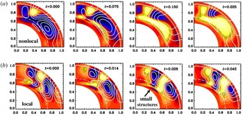
(a) Field lines in the meridional plane together with a colour-coded representation of the toroidal field (dark/blue shades indicate negative values and light/yellow shades positive values). Evolution of the field structure for model with near-surface shear layer using the $\unicode[STIX]{x2202}\overline{\boldsymbol{{\mathcal{E}}}}/\unicode[STIX]{x2202}t$ equation. (b) Same, but without the $\unicode[STIX]{x2202}\overline{\boldsymbol{{\mathcal{E}}}}/\unicode[STIX]{x2202}t$ equation. The magnetic cycle period is decreased from 0.53 to 0.11 diffusive times and the excitation conditions enhanced by a factor of five. Adapted from Brandenburg & Chatterjee (Reference Brandenburg and Chatterjee2018).

The beauty of the approach of using (2.18) lies in the fact that there is no problem in handling spherical geometry or even nonlinearities in an ad hoc manner such as $\unicode[STIX]{x1D6FC}$ quenching, as was already emphasized by Rheinhardt & Brandenburg (Reference Rheinhardt and Brandenburg2012). We say here ad hoc, because the original convolution is linear.

In figure 1 we show a comparison of two models of Brandenburg & Chatterjee (Reference Brandenburg and Chatterjee2018) in a spherical geometry with and without spatio-temporal non-locality. This model uses solar-like differential rotation contours and turbulent transport coefficients estimated from mean-field theory. It shows that spatio-temporal non-locality implies the absence of small structures, especially near the lower overshoot layer of the dynamo. Top and bottom panels cover half a period, so the panels on the right are similar to those on the left, except for a sign flip. The cycle period in the model with the $\unicode[STIX]{x2202}\overline{\boldsymbol{{\mathcal{E}}}}/\unicode[STIX]{x2202}t$ term included is 0.53 diffusion times, which is approximately five times longer than the period of 0.11 of the corresponding conventional models. For oscillatory solutions such as this one, temporal non-locality lowers the excitation conditions of the dynamo, as was already demonstrated by Rheinhardt & Brandenburg (Reference Rheinhardt and Brandenburg2012). In this example, the excitation conditions are lowered by a factor of approximately eight. Below, in § 2.8, we turn to the emergence of a completely new dynamo effect that occurs just owing to the presence of non-locality in time. Before this, however, we briefly explore the essence of the test-field method that led to the new insights regarding non-locality.

2.5 The test-field method: a way forward

Many of the detailed results discussed below would not have been discovered without the test-field method. We therefore briefly review in the following its basic aspects.

Analytic approaches have demonstrated the vast multitude of different effects, but they are limited in that, for turbulent flows with finite correlation times, they are only exact at low $R_{\text{m}}$ . Some methods such as the $\unicode[STIX]{x1D70F}$ approach are supposed to work at large $R_{\text{m}}$ , but they are not rigorous and always subject to numerical verification, using usually the test-field method.

In essence, the test-field method consists of solving equation (2.9) numerically, subject to given test fields $\overline{\boldsymbol{B}}^{T}$ , where the superscript $T$ denotes one of as many test fields as are needed to compute uniquely all elements of the $\unicode[STIX]{x1D6FC}_{ij}$ and $\unicode[STIX]{x1D702}_{ijk}$ tensors. In the following, we adopt $xy$ averaging, denoted by an overbar, and use the two test fields

(2.22a,b ) $$\begin{eqnarray}\overline{\boldsymbol{B}}^{T_{1}}=(\cos kz,0,0)\quad \text{and}\quad \overline{\boldsymbol{B}}^{T_{2}}=(\sin kz,0,0).\end{eqnarray}$$

For each of them, we find numerically a solution that we call correspondingly $\boldsymbol{b}^{T_{1}}(\boldsymbol{x},t)$ and $\boldsymbol{b}^{T_{2}}(\boldsymbol{x},t)$ . We then compute the corresponding mean electromotive force $\overline{\boldsymbol{{\mathcal{E}}}}^{T_{1}}=\overline{\boldsymbol{u}\times \boldsymbol{b}^{T_{1}}}$ and $\overline{\boldsymbol{{\mathcal{E}}}}^{T_{2}}=\overline{\boldsymbol{u}\times \boldsymbol{b}^{T_{2}}}$ . Inserting this into (2.8) yields

(2.23) $$\begin{eqnarray}\displaystyle & \displaystyle \overline{{\mathcal{E}}}_{i}^{T_{1}}=\overline{{\mathcal{E}}}_{i}^{(0)}+\unicode[STIX]{x1D6FC}_{i1}\cos kz-\unicode[STIX]{x1D702}_{i13}k\sin kz, & \displaystyle\end{eqnarray}$$

(2.24) $$\begin{eqnarray}\displaystyle & \displaystyle \overline{{\mathcal{E}}}_{i}^{T_{2}}=\overline{{\mathcal{E}}}_{i}^{(0)}+\unicode[STIX]{x1D6FC}_{i1}\sin kz+\unicode[STIX]{x1D702}_{i13}k\cos kz. & \displaystyle\end{eqnarray}$$

Here the last index of $\unicode[STIX]{x1D702}_{ijl}$ is $l=3$ , because $xy$ averages only depend on the third spatial coordinate, $z$ . To eliminate $\overline{{\mathcal{E}}}_{i}^{(0)}$ , we need solutions for the trivial test field $\overline{\boldsymbol{B}}^{T_{0}}=\mathbf{0}$ . The solutions $\boldsymbol{b}^{T_{0}}$ , and thus $\overline{\boldsymbol{{\mathcal{E}}}}^{(0)}$ , may then well be zero, but there are also cases where they are not – for example if the cross-helicity is finite; see Brandenburg & Rädler (Reference Brandenburg and Rädler2013).

We are now left with two pairs of unknown coefficients, $\unicode[STIX]{x1D6FC}_{i1}$ and $\unicode[STIX]{x1D702}_{i13}$ , for the two non-trivial cases $i=1$ and $i=2$ . (The third component of $xy$ -averaged mean fields is constant because $\unicode[STIX]{x1D735}\boldsymbol{\cdot }\overline{\boldsymbol{B}}=\overline{B}_{3,3}=0$ , so $\overline{B}_{3}=0$ if it vanished initially.) The two pairs of unknowns are readily obtained by solving a $2\times 2$ matrix problem with the solution (Brandenburg Reference Brandenburg2005b )

(2.25) $$\begin{eqnarray}\left(\begin{array}{@{}c@{}}\unicode[STIX]{x1D6FC}_{i1}\\ \unicode[STIX]{x1D702}_{i13}k\end{array}\right)=\left(\begin{array}{@{}cc@{}}\cos kz & \sin kz\\ -\text{sin}\,kz & \cos kz\end{array}\right)\left(\begin{array}{@{}c@{}}\overline{{\mathcal{E}}}_{i}^{T_{1}}-\overline{{\mathcal{E}}}_{i}^{(0)}\\ \overline{{\mathcal{E}}}_{i}^{T_{2}}-\overline{{\mathcal{E}}}_{i}^{(0)}\end{array}\right),\end{eqnarray}$$

which yields altogether four coefficients: $\unicode[STIX]{x1D6FC}_{11}$ , $\unicode[STIX]{x1D702}_{113}$ , $\unicode[STIX]{x1D6FC}_{21}$ and $\unicode[STIX]{x1D702}_{213}$ . To get the remaining four coefficients, $\unicode[STIX]{x1D6FC}_{12}$ , $\unicode[STIX]{x1D702}_{123}$ , $\unicode[STIX]{x1D6FC}_{22}$ and $\unicode[STIX]{x1D702}_{223}$ , we need two more test fields, $\overline{\boldsymbol{B}}^{T_{1}}=(0,\cos kz,0)$ and $\overline{\boldsymbol{B}}^{T_{2}}=(0,\sin kz,0)$ . Analogously to (2.25), this yields $(\unicode[STIX]{x1D6FC}_{i2},\unicode[STIX]{x1D702}_{i23}k)$ as the corresponding solution vector.

All these coefficients are generally also time dependent. For fluctuating fields, as is the case when $\boldsymbol{u}$ corresponds to turbulence, the coefficients are evidently also fluctuating. This can be relevant for studies of the incoherent $\unicode[STIX]{x1D6FC}$ -shear dynamo that will be discussed in § 5.3; see Brandenburg et al. (Reference Brandenburg, Rädler, Rheinhardt and Käpylä2008a ) for such applications. Another important case is where the test fields themselves are time dependent. In fact, this is of immediate relevance to all dynamo problems, where we expect the mean field to grow exponentially. Even for a simple turbulent decay problem, $\overline{\boldsymbol{B}}$ is time dependent: it is exponentially decaying. Both of these cases were considered by Hubbard & Brandenburg (Reference Hubbard and Brandenburg2009) using test fields proportional to $\text{e}^{st}$ or $\text{e}^{-\text{i}\unicode[STIX]{x1D714}t}$ with real coefficients $s$ and $\unicode[STIX]{x1D714}$ that they varied. This allowed them to assemble the functions $\unicode[STIX]{x1D6FC}_{ij}(\unicode[STIX]{x1D714})$ and $\unicode[STIX]{x1D702}_{ij3}(\unicode[STIX]{x1D714})$ , which led them to the results that for turbulent flows, both coefficients are, to lowest order, proportional to $1/(1-\text{i}\unicode[STIX]{x1D714}\unicode[STIX]{x1D70F})$ with $\unicode[STIX]{x1D70F}$ being some relaxation (or correlation) time, which is proportional to $(u_{\text{rms}}k_{\text{f}})^{-1}$ . The same result was obtained for test fields proportional to $\text{e}^{st}$ .

2.6 Alternative approaches to turbulent transport coefficients

It may be worth noting that there are a few other methods for computing $\unicode[STIX]{x1D6FC}_{ij}$ and $\unicode[STIX]{x1D702}_{ijl}$ . The simplest one is the imposed field method, which is exact in two dimensions and can then handle also fully nonlinear problems with magnetic background turbulence (Rheinhardt & Brandenburg Reference Rheinhardt and Brandenburg2010), as will be discussed in the next section. Instead of solving equation (2.9), one solves equation (2.1) in the presence of an imposed field. It was used to show that $\unicode[STIX]{x1D6FC}_{xx}$ and $\unicode[STIX]{x1D6FC}_{zz}$ can have opposite signs in rotating convection (Brandenburg et al. Reference Brandenburg, Nordlund, Pulkkinen, Stein and Tuominen1990). In three dimensions, however, turbulence makes the mean field non-uniform, so the actual electromotive force applies in reality to a problem with $\unicode[STIX]{x1D6FC}$ effect and turbulent diffusion while using just volume averages, as if there was no mean current density. Thus, this method is only of limited usefulness in three dimensions. A possible way out of this is to reset the fluctuations in regular intervals (Ossendrijver, Stix & Brandenburg Reference Ossendrijver, Stix and Brandenburg2001).

Another method assumes that, in a time-dependent turbulence simulation, $\overline{\boldsymbol{{\mathcal{E}}}}$ , $\overline{\boldsymbol{B}}$ and $\overline{\boldsymbol{J}}$ cover all possible states, allowing one to obtain all the coefficients of $\unicode[STIX]{x1D6FC}_{ij}$ and $\unicode[STIX]{x1D702}_{ijk}$ after averaging. This method has even been used to determine spatial non-locality (Brandenburg & Sokoloff Reference Brandenburg and Sokoloff2002), but it is not fully reliable, as was later demonstrated by comparing with the test-field method (Brandenburg Reference Brandenburg2005b ). Nevertheless, some success has been achieved in applications to accretion disk turbulence (Kowal, Otmianowska-Mazur & Hanasz Reference Kowal, Otmianowska-Mazur and Hanasz2006) and convection in spherical shells (Racine et al. Reference Racine, Charbonneau, Ghizaru, Bouchat and Smolarkiewicz2011; Simard, Charbonneau & Dubé Reference Simard, Charbonneau and Dubé2016); see Warnecke et al. (Reference Warnecke, Rheinhardt, Käpylä, Käpylä and Brandenburg2018) for a comparative assessment. Yet another method is multiscale stability theory (Lanotte et al. Reference Lanotte, Noullez, Vergassola and Wirth1999), which was recently shown to yield results equivalent to those of the test-field method (Andrievsky et al. Reference Andrievsky, Brandenburg, Noullez and Zheligovsky2015).

Many of the approaches developed for the induction equation are also applicable to the momentum equation, where turbulent viscosity, the anisotropic kinetic alpha (AKA) effect (Frisch, She & Sulem Reference Frisch, She and Sulem1987) and the $\unicode[STIX]{x1D6EC}$ effect (Rüdiger Reference Rüdiger1980) are prominent additions. Turbulent viscosity has been computed by determining the Reynolds stress in shear flows (e.g. Abramowicz, Brandenburg & Lasota Reference Abramowicz, Brandenburg and Lasota1996; Snellman et al. Reference Snellman, Käpylä, Korpi and Liljeström2009) or in decay experiments (Yousef, Brandenburg & Rüdiger Reference Yousef, Brandenburg and Rüdiger2003). On the other hand, by assuming the turbulent viscosity to be well approximated by $\unicode[STIX]{x1D708}_{\text{t}}\approx u_{\text{rms}}/3k_{\text{f}}$ , it has also been possible to estimate AKA and $\unicode[STIX]{x1D6EC}$ effects (Pulkkinen et al. Reference Pulkkinen, Tuominen, Brandenburg, Nordlund and Stein1993; Rieutord et al. Reference Rieutord, Brandenburg, Mangeney and Drossart1994; Brandenburg & von Rekowski Reference Brandenburg and von Rekowski2001; Karak et al. Reference Karak, Käpylä, Käpylä, Brandenburg, Olspert and Pelt2015; Käpylä Reference Käpylä2018). However, determining both $\unicode[STIX]{x1D708}_{\text{t}}$ and $\unicode[STIX]{x1D6EC}$ or AKA effects at the same time has not yet been successful.

An alternative or extension to mean-field theory in the usual sense is to solve the time-dependent system of one-point and two-point correlation functions. This approach goes by the name direct statistical simulations (Tobias & Marston Reference Tobias and Marston2013, Reference Tobias and Marston2017) and has been applied to two-dimensional turbulent shear flow problems. The dimensionality of the two-point correlation function doubles for those directions over which homogeneity cannot be assumed. On the other hand, the dynamics of the low-order statistics is usually slower than that of the original equations. In addition, it is possible to reduce the complexity of the problem by employing proper orthogonal decomposition (Allawala, Tobias & Marston Reference Allawala, Tobias and Marston2017). This approach has not yet been applied to magnetohydrodynamics and the dynamo problem, but it has the potential of being a strong competitor in addressing the high Reynolds number dynamics of problems of astrophysical and geophysical relevance.

2.7 From quasilinear to fully nonlinear test-field methods

The test-field equations are readily available in some publicly available codes, so for example in the Pencil Code Footnote ² (Brandenburg Reference Brandenburg2005b ) and in Nirvana Footnote ³ (Gressel et al. Reference Gressel, Ziegler, Elstner and Rüdiger2008a ; Gressel Reference Gressel2013). To newcomers in the field, it is always somewhat surprising that the test-field equations, i.e. equation (2.9) with $\overline{\boldsymbol{B}}$ being replaced by $\overline{\boldsymbol{B}}^{T}$ , can be solved without the magnetic field module being included at all. The reason is that the turbulent transport coefficients characterize just properties of the flow. Thus, the number of equations being solved is just the four or five hydrodynamic equations (either without or with energy equation included) together with the four versions of (2.9) for each of the four test fields – or more, if more test fields are needed (see Warnecke et al. Reference Warnecke, Rheinhardt, Käpylä, Käpylä and Brandenburg2018, for a case where nine vector equations were solved). However, if the magnetic field module is invoked, the magnetic field (which is different from the test fields) can grow and backreact onto the flow. Thus, one obtains turbulent transport coefficients that are modified by the magnetic field. This method is often referred to as the quasi-kinematic method and has been used on various occasions to the magnetic quenching of $\unicode[STIX]{x1D6FC}$ and $\unicode[STIX]{x1D702}_{\text{t}}$ (Brandenburg et al. Reference Brandenburg, Rädler, Rheinhardt and Subramanian2008b ; Karak et al. Reference Karak, Rheinhardt, Brandenburg, Käpylä and Käpylä2014). The limits of applicability of this method are still being investigated. Fully nonlinear approaches have been investigated; see Courvoisier, Hughes & Proctor (Reference Courvoisier, Hughes and Proctor2010) and Rheinhardt & Brandenburg (Reference Rheinhardt and Brandenburg2010). In those approaches, one also solves equation (2.19) for the fluctuating velocity.

The perhaps most striking counter example where the quasi-kinematic test-field method fails is that of a magnetically forced Roberts flow. This can easily be seen by computing the $\unicode[STIX]{x1D6FC}$ effect with the imposed field method in two dimensions, i.e. when there is no interference from turbulent diffusion or other terms. In such cases, the imposed field and fully nonlinear methods agree, while the quasi-kinematic method gives even the wrong sign of $\unicode[STIX]{x1D6FC}$ ; see Rheinhardt & Brandenburg (Reference Rheinhardt and Brandenburg2010) for details. Magnetically driven flows could in principle be realized by currents flowing through wires within the flow. This is a special situation that is not encountered in astrophysics. However, Rheinhardt & Brandenburg (Reference Rheinhardt and Brandenburg2010) speculated that flows exhibiting small-scale dynamo action could provide another example where the quasi-kinematic method fails, but this still needs to be demonstrated.

2.8 Dynamo effects from memory alone: Roberts flow III

Let us now discuss a remarkable result that has emerged by applying the test-field method to simple flow fields. The particular flow field considered here is referred to as Roberts flow III, which is one of a family of flows he studied (G. O. Roberts Reference Roberts1972). In Fourier space, as discussed in § 2.3, the non-locality in time corresponds to a division by $1-\text{i}\unicode[STIX]{x1D714}\unicode[STIX]{x1D70F}$ . This leads to an imaginary contribution in the dispersion relation that can turn a non-dynamo effect into a dynamo effect. An example is the pumping term, also known as turbulent diamagnetism (Zeldovich Reference Zeldovich1957; Rädler Reference Rädler1969). It corresponds to a contribution to $\overline{\boldsymbol{{\mathcal{E}}}}$ of the form $\unicode[STIX]{x1D738}\times \overline{\boldsymbol{B}}$ , where $\unicode[STIX]{x1D738}$ is a vector that leads to advection-like transport of the mean magnetic field without actual material motion. It corresponds to a transport down the gradient of turbulent intensity. We return to this aspect in § 3.5. Note also that the $\unicode[STIX]{x1D738}$ term corresponds to an off-diagonal contribution to the $\unicode[STIX]{x1D6FC}$ tensor of the form

(2.26) $$\begin{eqnarray}\unicode[STIX]{x1D6FC}_{ij}=-\unicode[STIX]{x1D716}_{ijk}\unicode[STIX]{x1D6FE}_{k}.\end{eqnarray}$$

Quite generally, the $\unicode[STIX]{x1D738}$ term implies that the dispersion relation for the complex growth rate $\unicode[STIX]{x1D706}(k)$ takes the form

(2.27) $$\begin{eqnarray}\unicode[STIX]{x1D706}(k)=-\text{i}\boldsymbol{k}\boldsymbol{\cdot }\unicode[STIX]{x1D738}-(\unicode[STIX]{x1D702}+\unicode[STIX]{x1D702}_{\text{t}})k^{2},\end{eqnarray}$$

where we have ignored other terms such as additional anisotropies, which do not enter for Roberts flow III.

Evidently, if we replace $\unicode[STIX]{x1D738}\rightarrow \unicode[STIX]{x1D738}^{(0)}/(1-\text{i}\unicode[STIX]{x1D714}\unicode[STIX]{x1D70F})$ , neglecting here the $k^{2}/k_{\text{f}}^{2}$ term from the spatial non-locality, and assuming $\unicode[STIX]{x1D714}\unicode[STIX]{x1D70F}\ll 1$ , then $-\text{i}\boldsymbol{k}\boldsymbol{\cdot }\unicode[STIX]{x1D738}\approx -\text{i}\boldsymbol{k}\boldsymbol{\cdot }\unicode[STIX]{x1D738}^{(0)}+\unicode[STIX]{x1D714}\unicode[STIX]{x1D70F}\boldsymbol{k}\boldsymbol{\cdot }\unicode[STIX]{x1D738}^{(0)}$ . Here, $\unicode[STIX]{x1D714}=\text{i}\unicode[STIX]{x1D706}$ is a complex frequency and is used interchangeably with $\text{i}\unicode[STIX]{x1D706}$ . Thus, there can be growth resulting from the second term if $\unicode[STIX]{x1D714}\unicode[STIX]{x1D70F}\boldsymbol{k}\boldsymbol{\cdot }\unicode[STIX]{x1D738}^{(0)}>\unicode[STIX]{x1D702}_{\text{t}}k^{2}$ . Such solutions are always oscillatory and show migratory dynamo waves in the direction of $\unicode[STIX]{x1D738}^{(0)}$ .

Solutions of the type discussed above have been found in direct numerical simulations of Roberts flow III (Rheinhardt et al. Reference Rheinhardt, Devlen, Rädler and Brandenburg2014). We now discuss the basic properties of one of their solutions in more detail. This flow is given by (G. O. Roberts Reference Roberts1972)

(2.28) $$\begin{eqnarray}\boldsymbol{u}=u_{0}\left(\begin{array}{@{}c@{}}\sin k_{0}x\,\cos k_{0}y\\ -\text{cos}\,k_{0}x\,\sin k_{0}y\\ \textstyle \frac{1}{2}(\cos 2k_{0}x+\cos 2k_{0}y)\end{array}\right)\quad \text{(Roberts flow III)},\end{eqnarray}$$

where $u_{0}$ is an amplitude factor and $k_{0}$ is the wavenumber of the flow. Both parameters enter in the definition of the magnetic Reynolds number, $R_{\text{m}}=u_{0}/\unicode[STIX]{x1D702}k_{0}$ . Rheinhardt et al. (Reference Rheinhardt, Devlen, Rädler and Brandenburg2014) found that dynamo action with a mean field proportional to $\exp [\text{i}(kz-\unicode[STIX]{x1D714}t)]$ is possible when $k/k_{0}\lesssim 0.78$ . This requires tall domains; in this case with $L_{z}/L_{x}=1/0.78$ . In the limit $k\rightarrow 0$ , there is large-scale dynamo action when $R_{\text{m}}\gtrsim 2.9$ . The mean field is oscillatory with a frequency that is at onset approximately $\unicode[STIX]{x1D714}\approx 0.037\,u_{0}k_{0}$ .

The marginally excited dynamo solution for Roberts flow III is already beyond the validity of SOCA, so the $\boldsymbol{u}\times \boldsymbol{b}-\overline{\boldsymbol{u}\times \boldsymbol{b}}$ term in (2.6) cannot be neglected. In fact, within the limitations of SOCA, which is only valid for small $R_{\text{m}}$ , no mean-field dynamo can be obtained for Roberts flow III. This is because, in the mean-field formalism, the $\unicode[STIX]{x1D6FE}$ term was found to emerge quadratically in $R_{\text{m}}$ , suggesting that it is a higher-order effect. Rheinhardt et al. (Reference Rheinhardt, Devlen, Rädler and Brandenburg2014) discussed in detail a particular example where $R_{\text{m}}=6$ and $k/k_{0}=0.4$ . The growth rate was found to be $0.047\,u_{0}k_{0}$ and the frequency was $0.29\,u_{0}k_{0}$ . In Fourier space, the turbulent magnetic diffusivity kernel was found to be $\unicode[STIX]{x1D702}_{\text{t}}(k,\unicode[STIX]{x1D714})=(0.21+0.03\,\text{i})\,u_{0}/k_{0}$ , which has only a small imaginary part corresponding to a weak memory effect, and $\unicode[STIX]{x1D6FE}(k,\unicode[STIX]{x1D714})=(0.73+0.27\,\text{i})\,u_{0}$ , which has a significant imaginary part corresponding to a strong memory effect. It is this term that is responsible for the positive growth rate. These complex coefficients match the dispersion relation given by (2.27) and reproduce the correct complex growth rate.

Describing spatio-temporal non-locality with an evolution equation for $\overline{\boldsymbol{{\mathcal{E}}}}$ is an approximation that is inaccurate for two reasons. First, in (2.17) there are in general higher powers of $k$ and $\unicode[STIX]{x1D714}$ , and second, the $k$ and $\unicode[STIX]{x1D714}$ dependencies of $\tilde{\unicode[STIX]{x1D6FC}}_{ij}$ and $\tilde{\unicode[STIX]{x1D702}}_{ijk}$ in (2.17) are usually not the same; see Rheinhardt et al. (Reference Rheinhardt, Devlen, Rädler and Brandenburg2014) for details. The main point of using such an approximation is to do better than just neglecting spatio-temporal non-locality altogether, as is still done in the vast majority of astrophysical applications. The differences are substantial, as was already demonstrated in figure 1. We see this again in the present example where the simple evolution equation (2.18) for $\overline{\boldsymbol{{\mathcal{E}}}}$ reproduces thus a qualitatively new dynamo effect.

2.9 Other Roberts flows and generalizations

In his original paper, G. O. Roberts (Reference Roberts1972) discussed altogether four flows. All the Roberts flows are two-dimensional with the same flow vectors in the horizontal $(x,y)$ directions, but different $xy$ patterns in the $z$ direction. His flow II is closely related to flow III discussed above; see Rheinhardt et al. (Reference Rheinhardt, Devlen, Rädler and Brandenburg2014) for details. It also leads to dynamo waves resulting from the off-diagonal terms $\unicode[STIX]{x1D6FC}_{xy}$ and $\unicode[STIX]{x1D6FC}_{yx}$ of the $\unicode[STIX]{x1D6FC}$ tensor with dynamo action owing to the memory term. The only difference is that here $\unicode[STIX]{x1D6FC}_{yx}=\unicode[STIX]{x1D6FC}_{xy}$ while for flow III we had $\unicode[STIX]{x1D6FC}_{yx}=-\unicode[STIX]{x1D6FC}_{xy}=\unicode[STIX]{x1D6FE}$ . Therefore, there are dynamo waves travelling in opposite directions for $\overline{B}_{x}$ and $\overline{B}_{y}$ .

Another interesting and very different example is Roberts flow IV, which is given by

(2.29) $$\begin{eqnarray}\boldsymbol{u}=u_{0}\left(\begin{array}{@{}c@{}}\sin k_{0}x\,\cos k_{0}y\\ -\text{cos}\,k_{0}x\,\sin k_{0}y\\ \sin k_{0}x\end{array}\right)\quad \text{(Roberts flow IV)}.\end{eqnarray}$$

It also produces large-scale magnetic fields that ‘survive’ horizontal averaging, but in this case the governing dispersion relation is just of the form

(2.30) $$\begin{eqnarray}\unicode[STIX]{x1D706}(k)=-[\unicode[STIX]{x1D702}+\unicode[STIX]{x1D702}_{\text{t}}(k)]k^{2},\end{eqnarray}$$

where $\unicode[STIX]{x1D702}_{\text{t}}(k)$ was found to be sufficiently negative for $k\lesssim 0.8\,k_{0}$ , but positive (corresponding to decay) for larger values of $k$ (Devlen, Brandenburg & Mitra Reference Devlen, Brandenburg and Mitra2013). Thus, on small length scales, the solution is always stable.

For completeness, let us mention that negative turbulent diffusivities can also be found for some compressible flows. However, in all those cases the destabilizing effect is never strong enough to overcome the microphysical value, i.e.  $\unicode[STIX]{x1D702}_{\text{t}}+\unicode[STIX]{x1D702}$ is still positive (Rädler et al. Reference Rädler, Brandenburg, Del Sordo and Rheinhardt2011).

The most famous Roberts flow is his flow I, because it is helical and therefore leads to an $\unicode[STIX]{x1D6FC}$ effect. Moreover, its helicity is maximal with $\overline{\unicode[STIX]{x1D74E}\boldsymbol{\cdot }\boldsymbol{u}}=k_{0}\,u_{0}^{2}$ . The flow is given by

(2.31) $$\begin{eqnarray}\boldsymbol{u}=u_{0}\left(\begin{array}{@{}c@{}}\sin (k_{0}x+\unicode[STIX]{x1D711}_{x})\,\cos (k_{0}y+\unicode[STIX]{x1D711}_{y})\\ -\text{cos}(k_{0}x+\unicode[STIX]{x1D711}_{x})\,\sin (k_{0}y+\unicode[STIX]{x1D711}_{y})\\ \sqrt{2}\sin (k_{0}x+\unicode[STIX]{x1D711}_{x})\,\sin (k_{0}y+\unicode[STIX]{x1D711}_{y})\end{array}\right)\quad (\text{Roberts flow I for }\unicode[STIX]{x1D711}_{x}=\unicode[STIX]{x1D711}_{y}=0),\end{eqnarray}$$

where $\unicode[STIX]{x1D711}_{x}=\unicode[STIX]{x1D711}_{y}=0$ will be assumed at first. This flow leads to a standard $\unicode[STIX]{x1D6FC}$ effect dynamo with a dispersion relation that is the same as for isotropic turbulence (Moffatt Reference Moffatt1970), namely

(2.32) $$\begin{eqnarray}\unicode[STIX]{x1D706}(k)=\pm |\unicode[STIX]{x1D6FC}\boldsymbol{k}|-[\unicode[STIX]{x1D702}+\unicode[STIX]{x1D702}_{\text{t}}]k^{2},\end{eqnarray}$$

where dynamo action is only possible for the upper sign. The dynamo is non-oscillatory. We return to $\unicode[STIX]{x1D6FC}$ effect dynamos further below, but before doing so, let us briefly discuss an interesting feature that arises when generalizing this flow to the case with time-dependent phases, as done by Galloway & Proctor (Reference Galloway and Proctor1992), who assumed

(2.33a,b ) $$\begin{eqnarray}\unicode[STIX]{x1D711}_{x}=\unicode[STIX]{x1D716}\cos \unicode[STIX]{x1D714}t,\quad \unicode[STIX]{x1D711}_{y}=\unicode[STIX]{x1D716}\sin \unicode[STIX]{x1D714}t,\end{eqnarray}$$

where $\unicode[STIX]{x1D716}$ and $\unicode[STIX]{x1D714}$ are additional parameters characterizing what is now generally referred to as the Galloway–Proctor flow. One normally considers a version of this flow that is rotated by $45^{\circ }$ , which allows one to fit two larger cells into the domain instead of the four cells in (2.31). This flow is a time-dependent generalization of Roberts flow I. This time dependence is of particular interest in that it allows the dynamo to become ‘fast’, which means that it can maintain a finite growth rate in the limit of large magnetic Reynolds numbers, $R_{\text{m}}=u_{\text{rms}}/\unicode[STIX]{x1D702}k_{\text{f}}\gg 1$ .

Numerical investigations of the Galloway–Proctor flow revealed the occurrence of an unexpected pumping effect, i.e.  $\unicode[STIX]{x1D738}\neq \mathbf{0}$ (Courvoisier, Hughes & Tobias Reference Courvoisier, Hughes and Tobias2006). This is because, owing to the circular polarization of this flow, the symmetry between $\boldsymbol{z}$ and $-\boldsymbol{z}$ is broken (Rädler & Brandenburg Reference Rädler and Brandenburg2009). Remarkably, such a $\unicode[STIX]{x1D6FE}$ effect does not emerge in the SOCA approximation which neglects the $\boldsymbol{u}\times \boldsymbol{b}-\overline{\boldsymbol{u}\times \boldsymbol{b}}$ term in (2.6). Numerical computations of $\unicode[STIX]{x1D6FE}$ with the test-field method showed that, indeed, for $R_{\text{m}}\rightarrow 0$ , one has $\unicode[STIX]{x1D6FE}\rightarrow 0$ . Furthermore, as $R_{\text{m}}\rightarrow 0$ , we have $|\unicode[STIX]{x1D6FE}|\propto R_{\text{m}}^{5}$ , which is a rather steep dependence. Analogously to the $\unicode[STIX]{x1D6FE}$ effect discussed in § 2.8, where $|\unicode[STIX]{x1D6FE}|$ increases quadratically with $R_{\text{m}}$ , this again suggests that this effect can only be described with a higher-order approximation in $R_{\text{m}}$ that is here higher than fourth order. Indeed, as shown by Rädler & Brandenburg (Reference Rädler and Brandenburg2009), a fourth-order approximation still does not capture this effect.

2.10 Horizontal averaging is not always suitable

Discontent with the use of horizontal averaging was expressed in the work of Gent et al. (Reference Gent, Shukurov, Fletcher, Sarson and Mantere2013a ,Reference Gent, Shukurov, Sarson, Fletcher and Mantere b ), who used averaging over a Gaussian kernel as an alternative. Ultimately, the usefulness of a particular averaging procedure can only be judged at the end, when we know the answer, what kind of large-scale field can be generated. The averaging procedure should be able to capture the expected class of large-scale fields. As an example, let us mention here a result of Devlen et al. (Reference Devlen, Brandenburg and Mitra2013), who did not find a negative eddy diffusivity dynamo for the Taylor–Green flow. This was indeed true for horizontal averaging, but not for vertical ( $z$ ) averaging, in which case the mean fields are two-dimensional. Such solutions were found by Andrievsky et al. (Reference Andrievsky, Brandenburg, Noullez and Zheligovsky2015), who presented several examples where the field survives $z$ averaging, but not $xy$ averaging. A related example was found by Bhat, Ebrahimi & Blackman (Reference Bhat, Ebrahimi and Blackman2016b ) using shearing box accretion disk simulations with a shear flow $u_{y}=Sx$ and $S=\text{const}$ They reported the emergence of different large-scale fields, depending on whether they employed $xy$ or $yz$ averaging.

The advantage of any of the averages discussed so far is that they obey the Reynolds rules. A practical example is azimuthal averaging in a sphere. However, such averaging fails to describe non-axisymmetric mean fields. Alternative averaging procedures such as spatial filtering are problematic in that they do not obey the Reynolds averaging rules; see Rädler (Reference Rädler1995, Reference Rädler2014). Ensemble averaging obeys the Reynolds rules and could describe non-axisymmetric mean fields, but the practical meaning of such averaging is unclear (Hoyng Reference Hoyng, Ferriz-Mas and Núñez2003). As will be discussed in § 4.4 in more detail, rapidly rotating stars with weak differential rotation are likely to exhibit non-axisymmetric mean fields. In that regime, the excitation conditions of such dynamos with an azimuthal order of $m=1$ are comparable to those of axisymmetric dynamos (Rädler Reference Rädler1980, Reference Rädler1986a ). Such solutions are now commonly found for rapidly rotating stars; see Viviani et al. (Reference Viviani, Warnecke, Käpylä, Käpylä, Olspert, Cole-Kodikara, Lehtinen and Brandenburg2018) for recent simulations.

2.11 Quenching of $\unicode[STIX]{x1D6FC}$ : self-inflicted anisotropy

As the magnetic field grows and its energy density becomes comparable to the kinetic energy density, the Lorentz force in the momentum equation begins to become important. This tends to decrease $\unicode[STIX]{x1D6FC}$ and $\unicode[STIX]{x1D702}_{\text{t}}$ in such a way as to saturate the dynamo. Assuming that our mean fields correspond to just planar averaging over the periodic $x$ and $y$ directions, they no longer depend on $x$ and $y$ . It is therefore clear that $\overline{\boldsymbol{B}}$ is just a function of $z$ and $t$ . Moreover, since $0=\unicode[STIX]{x1D735}\boldsymbol{\cdot }\overline{\boldsymbol{B}}=\overline{B}_{z,z}$ , we have $\overline{B}_{z}=\text{const.}$ and, unless $\overline{B}_{z}$ is initially finite, it must vanish at all later times. For a dynamo driven essentially by an $\unicode[STIX]{x1D6FC}$ effect, the $\overline{\boldsymbol{B}}$ with only $x$ and $y$ components must be an eigenfunction of the curl operator. This applies to all dynamos driven by a helical flow, such as the laminar Roberts flow I, and also to three-dimensional helical turbulence, for example. In a periodic domain $0<z<L_{z}$ , the eigenfunction is given by

(2.34) $$\begin{eqnarray}\overline{\boldsymbol{B}}=\left(\begin{array}{@{}c@{}}\sin (k_{1}z+\unicode[STIX]{x1D711})\\ \cos (k_{1}z+\unicode[STIX]{x1D711})\\ 0\end{array}\right),\end{eqnarray}$$

where $k_{1}=\pm 2\unicode[STIX]{x03C0}/L_{z}$ is the smallest wavenumber of the field in the $z$ direction and $\unicode[STIX]{x1D711}$ is an arbitrary phase which is only determined by the initial conditions. Note that $\unicode[STIX]{x1D735}\times \overline{\boldsymbol{B}}=k_{1}\overline{\boldsymbol{B}}$ , so $\overline{\boldsymbol{B}}$ is indeed an eigenfunction of the curl operator. The eigenvalue $k_{1}$ is positive (negative) if $\unicode[STIX]{x1D6FC}$ is positive (negative).

Once the magnetic field reaches equipartition strength with the flow, which we now assume to be driven by a forcing term in the momentum equation, the magnetic field saturates owing to the action of the Lorentz force in this momentum equation. The resulting changes to the flow begin to affect the $\unicode[STIX]{x1D6FC}$ tensor, which then inevitably attains an anisotropy proportional to $\overline{B}_{i}\overline{B}_{j}/\overline{\boldsymbol{B}}^{2}$ (Roberts Reference Roberts, Zahn and Zinn-Justin1993). We call this self-inflicted anisotropy. Thus, even if the $\unicode[STIX]{x1D6FC}$ tensor was initially isotropic (which is here the case in the $xy$ plane), it would become anisotropic at saturation and is then of the form

(2.35) $$\begin{eqnarray}\unicode[STIX]{x1D6FC}=\unicode[STIX]{x1D6FC}_{0}(\overline{B})\,\left(\begin{array}{@{}ccc@{}}1 & 0 & 0\\ 0 & 1 & 0\\ 0 & 0 & 0\end{array}\right)-\unicode[STIX]{x1D6FC}_{1}(\overline{B})\,\left(\begin{array}{@{}ccc@{}}\sin ^{2}k_{1}z & \sin k_{1}z\cos k_{1}z & 0\\ \sin k_{1}z\cos k_{1}z & \cos ^{2}k_{1}z & 0\\ 0 & 0 & 0\end{array}\right),\end{eqnarray}$$

where we have assumed $\unicode[STIX]{x1D711}=0$ for simplicity and $\overline{B}\equiv |\overline{\boldsymbol{B}}|$ because of $\sin ^{2}k_{1}z+\cos ^{2}k_{1}z=1$ , so the anisotropy is no longer apparent. Note that $\unicode[STIX]{x1D6FC}\overline{\boldsymbol{B}}=(\unicode[STIX]{x1D6FC}_{0}-\unicode[STIX]{x1D6FC}_{1})\overline{\boldsymbol{B}}$ . This form of $\unicode[STIX]{x1D6FC}$ with $\unicode[STIX]{x1D6FC}_{1}(\overline{B})$ having the opposite sign of $\unicode[STIX]{x1D6FC}_{0}(\overline{B})$ was confirmed by numerical simulations using the test-field method (Brandenburg et al. Reference Brandenburg, Rädler, Rheinhardt and Subramanian2008b ). Certain aspects of it were also verified with the imposed field method where one neglects the $\unicode[STIX]{x1D6FD}$ tensor and simply measures $\overline{\boldsymbol{{\mathcal{E}}}}=\langle \boldsymbol{u}\times \boldsymbol{b}\rangle$ in a simulation and computes then $\unicode[STIX]{x1D6FC}_{ij}$ from $\overline{{\mathcal{E}}}_{i}/\overline{B}_{j}$ (Hubbard et al. Reference Hubbard, Del Sordo, Käpylä and Brandenburg2009).

2.12 An insightful experiment with an independent induction equation

Cattaneo & Tobias (Reference Cattaneo and Tobias2009) were the first to study the nature of solutions to an independent induction equation,

(2.36) $$\begin{eqnarray}\frac{\unicode[STIX]{x2202}\boldsymbol{Z}}{\unicode[STIX]{x2202}t}=\unicode[STIX]{x1D735}\times (\boldsymbol{U}\times \boldsymbol{Z}-\unicode[STIX]{x1D702}\unicode[STIX]{x1D735}\times \boldsymbol{Z}),\end{eqnarray}$$

with a new vector field $\boldsymbol{Z}$ instead of $\boldsymbol{B}$ , but with the same quenched velocity field $\boldsymbol{U}(\boldsymbol{B})$ , which is the solution to the momentum equation with the usual Lorentz force $\boldsymbol{J}\times \boldsymbol{B}$ . The result was surprising in that the dynamo did not saturate by ‘relaxing the system to a state close to marginality or by suppressing the chaotic stretching in the flow’ (Cattaneo & Tobias Reference Cattaneo and Tobias2009). They argued further ‘that this process is very subtle and not in concord with any of the previously suggested theories’. Indeed, the naive expectation would be $\boldsymbol{Z}\propto \boldsymbol{B}$ , i.e. a field proportional to the one that led to the now saturated dynamo, whose flow we used in (2.36). However, the growth rate of such a $\boldsymbol{Z}$ would be exactly zero. In other words, we have

(2.37) $$\begin{eqnarray}\unicode[STIX]{x1D6FC}\overline{\boldsymbol{Z}}=\unicode[STIX]{x1D6FC}_{0}\overline{\boldsymbol{Z}},\quad \text{while }\unicode[STIX]{x1D6FC}\overline{\boldsymbol{B}}=(\unicode[STIX]{x1D6FC}_{0}-\unicode[STIX]{x1D6FC}_{1})\overline{\boldsymbol{B}}.\end{eqnarray}$$

Thus, if there were another solution that could actually grow under the influence of the velocity field $\boldsymbol{U}(\boldsymbol{B})$ , it would be the more preferred solution to (2.36). Given that $\boldsymbol{U}(\boldsymbol{B})$ is helical, we expect non-trivial horizontally averaged fields $\overline{\boldsymbol{Z}}$ to be a solution of the associated mean-field problem of (2.36), but with an $\unicode[STIX]{x1D6FC}$ tensor given still by (2.35), i.e. with $\overline{\boldsymbol{B}}$ rather than $\overline{\boldsymbol{Z}}$ . Given that $\unicode[STIX]{x1D6FC}_{1}(\overline{B})$ and $\unicode[STIX]{x1D6FC}_{0}(\overline{B})$ have opposite signs, an essential contribution to the quenching comes from the second term. Therefore, solutions $\overline{\boldsymbol{Z}}$ that belong to the null space of the matrix $\overline{B}_{i}\overline{B}_{j}$ would not be quenched by this term. This is indeed what Tilgner & Brandenburg (Reference Tilgner and Brandenburg2008) found; their $\overline{\boldsymbol{Z}}$ was a $90^{\circ }$ phase-shifted version of $\overline{\boldsymbol{B}}$ , i.e.  $\overline{\boldsymbol{Z}}(z)=\overline{\boldsymbol{B}}(z+\unicode[STIX]{x03C0}/2k_{1})$ . Indeed,

(2.38) $$\begin{eqnarray}\left(\begin{array}{@{}ccc@{}}\sin ^{2}k_{1}z & \sin k_{1}z\cos k_{1}z & 0\\ \sin k_{1}z\cos k_{1}z & \cos ^{2}k_{1}z & 0\\ 0 & 0 & 0\end{array}\right)\left(\begin{array}{@{}c@{}}\cos k_{1}z\\ -\text{sin}\,k_{1}z\\ 0\end{array}\right)=\mathbf{0},\end{eqnarray}$$

so this $\overline{\boldsymbol{Z}}$ is not being quenched by this second term in (2.35). Thus, $|\overline{\boldsymbol{Z}}|$ continues to grow exponentially. Some quenching might still occur because of a change of $\unicode[STIX]{x1D6FC}_{0}(\overline{B})$ , but in the experiments of Tilgner & Brandenburg (Reference Tilgner and Brandenburg2008), this effect was small. This remarkable, but perfectly understandable behaviour in the evolution of $|\overline{\boldsymbol{Z}}|$ provides another independent verification of the quenching expression given by (2.35).

2.13 Catastrophic quenching

Early work with the imposed field method using a uniform magnetic field $\boldsymbol{B}_{0}=\text{const.}$ resulted in an $\unicode[STIX]{x1D6FC}$ effect whose value seemed to be quenched in an $R_{\text{m}}$ -dependent fashion. Blackman & Field (Reference Blackman and Field2000a ) called this catastrophic quenching, because $\unicode[STIX]{x1D6FC}$ would be catastrophically small in the astrophysically relevant case of large $R_{\text{m}}$ . This was first suggested by Vainshtein & Cattaneo (Reference Vainshtein and Cattaneo1992) and confirmed numerically by Cattaneo & Hughes (Reference Cattaneo and Hughes1996). This result irritated the astrophysics community for some time. Indeed, it seemed a bit like a crisis to all of mean-field theory and, maybe, we would not have had this special edition of the Journal of Plasma Physics (JPP) if this quenching was really as catastrophic as it seemed at the time!

The solution to the catastrophic quenching problem turned out to be another highlight of dynamo theory and has its roots in an early finding by Pouquet, Frisch & Léorat (Reference Pouquet, Frisch and Léorat1976). They realized that, in the nonlinear case at sufficiently large $R_{\text{m}}$ , the $\unicode[STIX]{x1D6FC}$ effect has a new contribution which is not just proportional to the mean kinetic helicity density $\overline{\unicode[STIX]{x1D74E}\boldsymbol{\cdot }\boldsymbol{u}}$ , as stated in the beginning in (2.12), but there is a term proportional to the mean current helicity density from the fluctuating fields $\overline{\boldsymbol{j}\boldsymbol{\cdot }\boldsymbol{b}}$ , where $\boldsymbol{j}=\unicode[STIX]{x1D735}\times \boldsymbol{b}/\unicode[STIX]{x1D707}_{0}$ is the small-scale current density. This term emerges naturally from the $\overline{\dot{\boldsymbol{u}}\times \boldsymbol{b}}$ term in (2.20) when using the $\unicode[STIX]{x1D70F}$ approximation; see § 2.4. Thus, we have (Pouquet et al. Reference Pouquet, Frisch and Léorat1976)

(2.39) $$\begin{eqnarray}\unicode[STIX]{x1D6FC}_{0}=-\textstyle \frac{1}{3}\unicode[STIX]{x1D70F}(\overline{\unicode[STIX]{x1D74E}\boldsymbol{\cdot }\boldsymbol{u}}-\overline{\boldsymbol{j}\boldsymbol{\cdot }\boldsymbol{b}}/\overline{\unicode[STIX]{x1D70C}}),\end{eqnarray}$$

where $\overline{\unicode[STIX]{x1D70C}}$ is the mean fluid density. However, if the small-scale magnetic field is still approximately statistically isotropic, the small-scale current helicity, $\overline{\boldsymbol{j}\boldsymbol{\cdot }\boldsymbol{b}}$ , must be approximately $k_{\text{f}}^{2}\,\overline{\boldsymbol{a}\boldsymbol{\cdot }\boldsymbol{b}}/\unicode[STIX]{x1D707}_{0}$ , where $\boldsymbol{a}$ is the magnetic vector potential of the small-scale field, $\boldsymbol{b}=\unicode[STIX]{x1D735}\times \boldsymbol{a}$ . Interestingly, $\overline{\boldsymbol{a}\boldsymbol{\cdot }\boldsymbol{b}}$ is constrained, on the one hand, by $\overline{\boldsymbol{A}\boldsymbol{\cdot }\boldsymbol{B}}$ , i.e. the mean magnetic helicity density of the total field, which obeys a conservation equation, and on the other hand by $\overline{\boldsymbol{A}}\boldsymbol{\cdot }\overline{\boldsymbol{B}}$ , which is the result of the mean-field dynamo problem (Hubbard & Brandenburg Reference Hubbard and Brandenburg2012), i.e.

(2.40) $$\begin{eqnarray}\frac{\unicode[STIX]{x2202}}{\unicode[STIX]{x2202}t}\overline{\boldsymbol{A}}\boldsymbol{\cdot }\overline{\boldsymbol{B}}=2\overline{\boldsymbol{{\mathcal{E}}}}\boldsymbol{\cdot }\overline{\boldsymbol{B}}-2\unicode[STIX]{x1D702}\unicode[STIX]{x1D707}_{0}\overline{\boldsymbol{J}}\boldsymbol{\cdot }\overline{\boldsymbol{B}}-\unicode[STIX]{x1D735}\boldsymbol{\cdot }(\overline{\boldsymbol{F}}_{\text{m}}-\overline{\boldsymbol{{\mathcal{E}}}}\times \overline{\boldsymbol{A}}),\end{eqnarray}$$

where $\overline{\boldsymbol{F}}_{\text{m}}$ is the magnetic helicity flux from the large-scale field and $\overline{\boldsymbol{E}}=\unicode[STIX]{x1D702}\unicode[STIX]{x1D707}_{0}\overline{\boldsymbol{J}}-\overline{\boldsymbol{U}}\times \overline{\boldsymbol{B}}$ is the mean electric field without the $\overline{\boldsymbol{{\mathcal{E}}}}$ term. Thus, $\overline{\boldsymbol{a}\boldsymbol{\cdot }\boldsymbol{b}}$ must obey the equation (Kleeorin & Ruzmaikin Reference Kleeorin and Ruzmaikin1982; Kleeorin et al. Reference Kleeorin, Moss, Rogachevskii and Sokoloff2000)

(2.41) $$\begin{eqnarray}\frac{\unicode[STIX]{x2202}}{\unicode[STIX]{x2202}t}\overline{\boldsymbol{a}\boldsymbol{\cdot }\boldsymbol{b}}=-2\overline{\boldsymbol{{\mathcal{E}}}}\boldsymbol{\cdot }\overline{\boldsymbol{B}}-2\unicode[STIX]{x1D702}\unicode[STIX]{x1D707}_{0}\,\overline{\boldsymbol{j}\boldsymbol{\cdot }\boldsymbol{b}}-\unicode[STIX]{x1D735}\boldsymbol{\cdot }(\overline{\boldsymbol{F}}_{\text{f}}+\overline{\boldsymbol{{\mathcal{E}}}}\times \overline{\boldsymbol{A}}),\end{eqnarray}$$

so that the sum of (2.40) and (2.41) is equal to

(2.42) $$\begin{eqnarray}\frac{\unicode[STIX]{x2202}}{\unicode[STIX]{x2202}t}\overline{\boldsymbol{A}\boldsymbol{\cdot }\boldsymbol{B}}=-2\unicode[STIX]{x1D702}\unicode[STIX]{x1D707}_{0}\,\overline{\boldsymbol{J}\boldsymbol{\cdot }\boldsymbol{B}}-\unicode[STIX]{x1D735}\boldsymbol{\cdot }\overline{\boldsymbol{F}}_{\text{tot}},\end{eqnarray}$$

where $\overline{\boldsymbol{F}}_{\text{tot}}=\overline{\boldsymbol{F}}_{\text{m}}+\overline{\boldsymbol{F}}_{\text{f}}$ is the sum of magnetic helicity fluxes from the mean and fluctuating fields, respectively. Equation (2.41) can easily be formulated as an evolution equation for $\unicode[STIX]{x1D6FC}$ , or at least its magnetic contribution, as was first done by Kleeorin & Ruzmaikin (Reference Kleeorin and Ruzmaikin1982).

A few additional comments are here in order. First, analogous to the pair of terms $\pm 2\overline{\boldsymbol{{\mathcal{E}}}}\boldsymbol{\cdot }\overline{\boldsymbol{B}}$ in (2.40) and (2.41), we have isolated the pair $\mp \overline{\boldsymbol{{\mathcal{E}}}}\times \overline{\boldsymbol{A}}$ underneath the corresponding flux divergence terms. This was first done by Hubbard & Brandenburg (Reference Hubbard and Brandenburg2012), who found these to give important contributions, especially to the flux in the equation for the small-scale magnetic helicity. This term complements a corresponding term of opposite sign in the equation for the large-scale magnetic helicity, but it does not contribute to the total magnetic helicity flux. Second, it can be advantageous to solve directly the equation for the total magnetic helicity flux, as done by Hubbard & Brandenburg (Reference Hubbard and Brandenburg2012). This ensures that mutually cancelling terms do not contribute ‘accidently’ (as a result of inaccurate approximations) to the total magnetic helicity flux. This approach has been adopted by Pipin et al. (Reference Pipin, Sokoloff, Zhang and Kuzanyan2013a ,Reference Pipin, Zhang, Sokoloff, Kuzanyan and Gao b ) and Pipin & Kosovichev (Reference Pipin and Kosovichev2013, Reference Pipin and Kosovichev2016) to model the solar dynamo; see also Pipin (Reference Pipin2015, Reference Pipin2017).

When formulated as an evolution equation for $\unicode[STIX]{x1D6FC}$ , the approach described above is referred to as ‘dynamical’ quenching. This is not an alternative to the ‘algebraic’ quenching, which describes the functional dependencies of $\unicode[STIX]{x1D6FC}_{0}(\overline{B})$ and $\unicode[STIX]{x1D6FC}_{1}(\overline{B})$ in (2.35), but it is an additional contribution to $\unicode[STIX]{x1D6FC}_{0}(\overline{B})$ , and has in principle also additional anisotropic contributions (Rogachevskii & Kleeorin Reference Rogachevskii and Kleeorin2007; Pipin Reference Pipin2008). It provides a feedback from the growing or evolving $\overline{\boldsymbol{A}}\boldsymbol{\cdot }\overline{\boldsymbol{B}}$ that is necessary to obey the total magnetic helicity equation (2.42).

As pointed out by Rädler & Rheinhardt (Reference Rädler and Rheinhardt2007), dynamical quenching has not been derived rigorously within mean-field theory, and must rather be regarded as a heuristic approach. Dynamical quenching does not emerge in the traditional approach of solving for the fluctuations. One should expect that the magnetic helicity equation would automatically be obeyed if one solved the equations for the fluctuations by avoiding questionable approximations. At present, however, dynamical quenching is the only known approach that describes correctly the resistively slow saturation of $\unicode[STIX]{x1D6FC}^{2}$ dynamos in triply periodic domains (Blackman & Brandenburg Reference Blackman and Brandenburg2002; Field & Blackman Reference Field and Blackman2002; Subramanian Reference Subramanian2002) found by Brandenburg (Reference Brandenburg2001), as will be discussed in § 2.14.

The aforementioned simulations were done with helically forced turbulence, which led, at late times, to the development of a large-scale magnetic field of Beltrami type; see equation (2.34) for one such example, where the wavevector of the mean field points in the $z$ direction. In figure 2 we show an example of the gradual approach to such a Beltrami field, which has here a wavevector pointing in the $x$ direction.

Figure 2.

Visualizations of $B_{x}/B_{\text{eq}}$ on the periphery of the domain at six times during the late saturation stage of the dynamo when a large-scale field is gradually building up. The small-scale field has reached its final value after $t/\unicode[STIX]{x1D70F}\approx 100$ turnover times. The diffusive time is here approximately 7000 times the turnover time. The maximum field strength is approximately twice $B_{\text{eq}}$ .

The evolution equation for $\unicode[STIX]{x1D6FC}$ can also be written in implicit form with the time derivative of $\unicode[STIX]{x1D6FC}$ on the right-hand side as (Brandenburg Reference Brandenburg2008)

(2.43) $$\begin{eqnarray}\unicode[STIX]{x1D6FC}=\frac{\unicode[STIX]{x1D6FC}_{\text{K}}+R_{\text{m}}[\unicode[STIX]{x1D702}_{\text{t}}\unicode[STIX]{x1D707}_{0}\,\overline{\boldsymbol{J}}\boldsymbol{\cdot }\overline{\boldsymbol{B}}/B_{\text{eq}}^{2}-(\unicode[STIX]{x1D735}\boldsymbol{\cdot }\overline{\boldsymbol{F}}_{\text{f}})/(2B_{\text{eq}}^{2})-(\unicode[STIX]{x2202}\unicode[STIX]{x1D6FC}/\unicode[STIX]{x2202}t)/(2\unicode[STIX]{x1D702}_{\text{t}}k_{\text{f}}^{2})]}{1+R_{\text{m}}\overline{\boldsymbol{B}}^{2}/B_{\text{eq}}^{2}},\end{eqnarray}$$

where $\unicode[STIX]{x1D6FC}_{\text{K}}$ is the $\unicode[STIX]{x1D6FC}$ effect in the kinematic limit. The formulation in (2.43) confirms first of all the early catastrophic quenching result of Vainshtein & Cattaneo (Reference Vainshtein and Cattaneo1992) for volume-averaged mean fields, because those are independent of the spatial coordinates and, therefore, $\unicode[STIX]{x1D707}_{0}\,\overline{\boldsymbol{J}}=\unicode[STIX]{x1D735}\times \overline{\boldsymbol{B}}=\mathbf{0}$ . The periodicity implies $\unicode[STIX]{x1D735}\boldsymbol{\cdot }\overline{\boldsymbol{F}}_{\text{f}}=0$ . Also, they considered a stationary state, so $\unicode[STIX]{x2202}\unicode[STIX]{x1D6FC}/\unicode[STIX]{x2202}t=0$ . Thus, all the factors of $R_{\text{m}}$ in the numerator vanish and therefore we have $\unicode[STIX]{x1D6FC}=\unicode[STIX]{x1D6FC}_{\text{K}}/(1+R_{\text{m}}\overline{\boldsymbol{B}}^{2}/B_{\text{eq}}^{2})$ , as predicted by Vainshtein & Cattaneo (Reference Vainshtein and Cattaneo1992). In general, however, the presence of any of the three additional terms in the numerator multiply $R_{\text{m}}$ and are therefore of the same order as those in the denominator. This should readily alleviate the threat of an $R_{\text{m}}$ -dependent quenching. Interestingly, equation (2.43) applies also when the dynamo is not driven by the $\unicode[STIX]{x1D6FC}_{\text{K}}$ term, but by the shear–current effect, for example (Brandenburg & Subramanian Reference Brandenburg and Subramanian2005b ). Thus, somewhat paradoxically, we could say that an $\unicode[STIX]{x1D6FC}$ effect can be quenched even if there is no $\unicode[STIX]{x1D6FC}$ to begin with.

In the absence of magnetic helicity fluxes, i.e. when $\unicode[STIX]{x1D735}\boldsymbol{\cdot }\overline{\boldsymbol{F}}_{\text{f}}=0$ , as in the present case of homogeneous turbulence with periodic boundary conditions, the time evolution is inevitably controlled by a resistively slow term. This somewhat surprising constraint for homogeneous helical turbulence can be understood quite generally – even without resorting to any mean-field theory, i.e. without talking about $\unicode[STIX]{x1D6FC}$ effect and turbulent magnetic diffusivity. This will be discussed next.

2.14 Resistively slow saturation in homogeneous turbulence

To describe the late saturation phase, we invoke the magnetic helicity equation for the whole volume, which is assumed to be either periodic or embedded in a perfect conductor. Volume averages will be denoted by angle brackets. Thus, we have

(2.44) $$\begin{eqnarray}\frac{\text{d}}{\text{d}t}\langle \boldsymbol{A}\boldsymbol{\cdot }\boldsymbol{B}\rangle =-2\unicode[STIX]{x1D702}\unicode[STIX]{x1D707}_{0}\langle \boldsymbol{J}\boldsymbol{\cdot }\boldsymbol{B}\rangle ,\end{eqnarray}$$

which is the same as equation (2.42), but without the magnetic helicity flux divergence term. (For the volume averages employed here, this would lead to a surface term, which vanishes for periodic or perfectly conducting boundaries.) This equation highlights an important result for the steady state, namely

(2.45) $$\begin{eqnarray}\langle \boldsymbol{J}\boldsymbol{\cdot }\boldsymbol{B}\rangle =0\quad \text{(for any steady state in triply periodic domains)}.\end{eqnarray}$$

This sounds somewhat boring, but becomes immediately interesting when realizing that mean fields and fluctuations can both be finite, i.e.

(2.46) $$\begin{eqnarray}\langle \boldsymbol{j}\boldsymbol{\cdot }\boldsymbol{b}\rangle =-\langle \overline{\boldsymbol{J}}\boldsymbol{\cdot }\overline{\boldsymbol{B}}\rangle \neq 0,\end{eqnarray}$$

so that $\langle \boldsymbol{J}\boldsymbol{\cdot }\boldsymbol{B}\rangle =\langle \overline{\boldsymbol{J}}\boldsymbol{\cdot }\overline{\boldsymbol{B}}\rangle +\langle \boldsymbol{j}\boldsymbol{\cdot }\boldsymbol{b}\rangle =0$ , as required.

To describe the gradual approach to the stationary state given by (2.45), we have to retain the time derivative in (2.44). Writing $\langle \boldsymbol{A}\boldsymbol{\cdot }\boldsymbol{B}\rangle =\langle \overline{\boldsymbol{A}}\boldsymbol{\cdot }\overline{\boldsymbol{B}}\rangle +\langle \boldsymbol{a}\boldsymbol{\cdot }\boldsymbol{b}\rangle$ , and assuming that, in the late saturation phase, the quadratic correlations of the fluctuations are already constant and only the correlations of mean fields are not, we can omit the time derivative of $\langle \boldsymbol{a}\boldsymbol{\cdot }\boldsymbol{b}\rangle$ . Furthermore, we assume magnetic fields with positive (negative) magnetic helicity at small scales, i.e.

(2.47) $$\begin{eqnarray}\unicode[STIX]{x1D707}_{0}\langle \boldsymbol{j}\boldsymbol{\cdot }\boldsymbol{b}\rangle \approx \pm k_{\text{f}}\langle \boldsymbol{b}^{2}\rangle \approx k_{\text{f}}^{2}\langle \boldsymbol{a}\boldsymbol{\cdot }\boldsymbol{b}\rangle ,\end{eqnarray}$$

and that $\langle \boldsymbol{b}^{2}\rangle \approx \unicode[STIX]{x1D707}_{0}\langle \unicode[STIX]{x1D70C}\boldsymbol{u}^{2}\rangle \equiv B_{\text{eq}}^{2}$ , which is the square of the equipartition value. Here, the upper (lower) signs refer to positive (negative) magnetic helicity at small scales. Furthermore, owing to (2.34), we have

(2.48) $$\begin{eqnarray}\overline{\boldsymbol{J}}\boldsymbol{\cdot }\overline{\boldsymbol{B}}=\mp k_{1}\overline{\boldsymbol{B}}^{2}=k_{1}^{2}\,\overline{\boldsymbol{A}}\boldsymbol{\cdot }\overline{\boldsymbol{B}},\end{eqnarray}$$

which is, for pure modes with wavenumber $k_{1}$ , constant in space. However, this relation is no longer exact for a superposition of modes. Thus, with these provisions, equation (2.44) becomes (Brandenburg Reference Brandenburg2001)

(2.49) $$\begin{eqnarray}\frac{\text{d}}{\text{d}t}\langle \overline{\boldsymbol{B}}^{2}\rangle =2\unicode[STIX]{x1D702}k_{1}k_{\text{f}}B_{\text{eq}}^{2}-2\unicode[STIX]{x1D702}k_{1}^{2}\langle \overline{\boldsymbol{B}}^{2}\rangle ,\end{eqnarray}$$

with the solution

(2.50) $$\begin{eqnarray}\langle \overline{\boldsymbol{B}}^{2}\rangle =B_{\text{eq}}^{2}\frac{k_{\text{f}}}{k_{1}}[1-\text{e}^{-2\unicode[STIX]{x1D702}k_{1}^{2}(t-t_{\text{sat}})}].\end{eqnarray}$$

This agrees with the slow saturation behaviour seen first in the simulations of Brandenburg (Reference Brandenburg2001); see figure 3. Here $t_{\text{sat}}$ is the time when the slow saturation phase commences; see the crossing of the green dashed line with the abscissa. Interestingly, instead of waiting until full saturation is accomplished, one can obtain the saturation value already much earlier simply by differentiating the simulation data to compute (Candelaresi & Brandenburg Reference Candelaresi and Brandenburg2013)

(2.51) $$\begin{eqnarray}B_{\text{sat}}^{2}\approx \langle \overline{\boldsymbol{B}}^{2}\rangle +\unicode[STIX]{x1D70F}_{\text{diff}}\frac{\text{d}}{\text{d}t}\langle \overline{\boldsymbol{B}}^{2}\rangle .\end{eqnarray}$$

Note that the inverse time constant $\unicode[STIX]{x1D70F}_{\text{diff}}^{-1}=2\unicode[STIX]{x1D702}k_{1}^{2}$ in the exponent of (2.50) is fixed by the microphysics and does not involve the turbulent magnetic diffusivity. This is therefore still in some sense catastrophic, so real astrophysical dynamos do not work like this, and this is because of magnetic helicity fluxes. To demonstrate this in a really convincing way requires simulations at magnetic Reynolds numbers well in excess of 1000 (Del Sordo, Guerrero & Brandenburg Reference Del Sordo, Guerrero and Brandenburg2013). We discuss magnetic helicity fluxes next.

Figure 3.

Evolution of the normalized $\langle \overline{\boldsymbol{B}}^{2}\rangle$ and that of $\langle \overline{\boldsymbol{B}}^{2}\rangle +\unicode[STIX]{x1D70F}_{\text{diff}}\text{d}\langle \overline{\boldsymbol{B}}^{2}\rangle /\text{d}t$ (dotted), compared with its average in the interval $1.2\leqslant t/\unicode[STIX]{x1D70F}_{\text{diff}}\leqslant 3.5$ (horizontal blue solid line), as well as averages over three subintervals (horizontal red dashed lines). The green dashed line corresponds to (2.50) with $t_{\text{sat}}/\unicode[STIX]{x1D70F}_{\text{diff}}=0.54$ .

2.15 Magnetic helicity fluxes

The most important contribution to the magnetic helicity flux is a turbulent diffusive flux proportional to the negative gradient of the magnetic helicity density (Hubbard & Brandenburg Reference Hubbard and Brandenburg2010), i.e.

(2.52) $$\begin{eqnarray}\overline{\boldsymbol{F}}_{\text{f}}=-\unicode[STIX]{x1D705}_{h}\unicode[STIX]{x1D735}\overline{\boldsymbol{a}\boldsymbol{\cdot }\boldsymbol{b}}.\end{eqnarray}$$

Such a formulation raises immediately the question of the gauge dependence of magnetic helicity. This turns out to be less of an issue than originally anticipated. A first step in this realization comes from the work of Subramanian & Brandenburg (Reference Subramanian and Brandenburg2006), who showed that the magnetic helicity density can be expressed in terms of a density of linkages, provided the correlation scale is much smaller than the mean field or system scale. In reality, of course, a broad range of length scales will be excited, and this can be described by the (shell-integrated) magnetic helicity spectrum, $H_{\text{M}}(k)$ , which is normalized such that $\int H_{\text{M}}(k)\,\text{d}k=\langle \boldsymbol{A}\boldsymbol{\cdot }\boldsymbol{B}\rangle$ . For a general review on astrophysical turbulence discussing also spectra such as these, see Brandenburg & Nordlund (Reference Brandenburg and Nordlund2011).

Magnetic helicity spectra have been obtained from solar observations (Zhang, Brandenburg & Sokoloff Reference Zhang, Brandenburg and Sokoloff2014, Reference Zhang, Brandenburg and Sokoloff2016; Brandenburg, Petrie & Singh Reference Brandenburg, Petrie and Singh2017c ) and even for the solar wind (Matthaeus & Goldstein Reference Matthaeus and Goldstein1982; Brandenburg et al. Reference Brandenburg, Subramanian, Balogh and Goldstein2011b ), as will be discussed below. Such spectra are automatically gauge invariant owing to the implicit assumption that, by taking a Fourier transform, one assumes a periodic domain. Clearly, this is unrealistic on the largest scales, but this only affects the magnetic helicity spectra at the smallest wavenumbers. At all other wavenumbers, the spectrum should be a physically meaningful quantity and the same in any gauge.

Figure 4.

Time-averaged profiles of $\langle \overline{\boldsymbol{{\mathcal{E}}}}\boldsymbol{\cdot }\overline{\boldsymbol{B}}\rangle$ and $\unicode[STIX]{x1D702}\langle \boldsymbol{j}\boldsymbol{\cdot }\boldsymbol{b}\rangle$ (a), the difference between these terms compared with the magnetic helicity flux divergence of small-scale fields $\langle \unicode[STIX]{x1D735}\boldsymbol{\cdot }\overline{\boldsymbol{F}}_{\text{f}}\rangle$ (b) and the flux itself compared with the Fickian diffusion ansatz (c). The fluxes are in given in units of $\unicode[STIX]{x1D702}_{\text{t0}}B_{\text{eq}}^{2}$ and the flux divergence is given in units of $k_{1}\unicode[STIX]{x1D702}_{\text{t0}}B_{\text{eq}}^{2}$ .

Measurements of magnetic helicity fluxes have been performed by Hubbard & Brandenburg (Reference Hubbard and Brandenburg2010) for an $\unicode[STIX]{x1D6FC}^{2}$ dynamo embedded in a poorly conducting halo and by Del Sordo et al. (Reference Del Sordo, Guerrero and Brandenburg2013) for a dynamo with a wind so one can compare turbulent–diffusive and advective fluxes. Mitra et al. (Reference Mitra, Candelaresi, Chatterjee, Tavakol and Brandenburg2010b ) have explicitly demonstrated the gauge independence of the small-scale magnetic helicity flux by working in three different gauges. In all those cases, it was found that the magnetic helicity flux divergence is comparable to the Spitzer magnetic helicity production, $2\unicode[STIX]{x1D702}\unicode[STIX]{x1D707}_{0}\overline{\boldsymbol{j}\boldsymbol{\cdot }\boldsymbol{b}}$ . In figure 4, we show time-averaged profiles of $2\overline{\boldsymbol{{\mathcal{E}}}}\boldsymbol{\cdot }\overline{\boldsymbol{B}}$ and $2\unicode[STIX]{x1D702}\overline{\boldsymbol{j}\boldsymbol{\cdot }\boldsymbol{b}}$ , as well as the difference between these two terms compared with the magnetic helicity flux divergence of small-scale fields, $\unicode[STIX]{x1D735}\boldsymbol{\cdot }\overline{\boldsymbol{F}}_{\text{f}}$ , and the flux itself compared with the Fickian diffusion ansatz for the model of Hubbard & Brandenburg (Reference Hubbard and Brandenburg2010) at $R_{\text{m}}\approx 270$ . We see that the magnetic helicity flux divergence of small-scale fields is still less than the magnetic helicity production by the mean electromotive. Thus, the magnetic helicity flux divergence is still subdominant. It can therefore not yet alleviate the resistively slow saturation of the dynamo. One might hope that this will change at larger values of $R_{\text{m}}$ . As of now, however, it has not yet been possible to demonstrate this convincingly.

Most of the dynamo simulations to date are not yet in the asymptotic regime where $R_{\text{m}}$ is large enough to alleviate resistively slow saturation. It would be important to demonstrate more thoroughly to what extent those dynamos are in the asymptotic regime, and that

(2.53) $$\begin{eqnarray}|\unicode[STIX]{x1D735}\boldsymbol{\cdot }\overline{\boldsymbol{F}}_{\text{f}}|\approx |2\overline{\boldsymbol{{\mathcal{E}}}}\boldsymbol{\cdot }\overline{\boldsymbol{B}}|\gg |2\unicode[STIX]{x1D702}\unicode[STIX]{x1D707}_{0}\overline{\boldsymbol{j}\boldsymbol{\cdot }\boldsymbol{b}}|,\end{eqnarray}$$

as one should expect. Let us emphasize here that, unlike the flux divergence $\unicode[STIX]{x1D735}\boldsymbol{\cdot }\overline{\boldsymbol{F}}_{\text{f}}$ , the actual helicity fluxes can always be gauged such that they vanish across an impenetrable boundary by adopting the gauge $\boldsymbol{U}\boldsymbol{\cdot }\boldsymbol{A}=0$ (Candelaresi et al. Reference Candelaresi, Hubbard, Brandenburg and Mitra2011). In that case, the magnetic helicity density evolves just like a passive scaler, i.e.

(2.54) $$\begin{eqnarray}\frac{\unicode[STIX]{x2202}}{\unicode[STIX]{x2202}t}\boldsymbol{A}\boldsymbol{\cdot }\boldsymbol{B}=-\unicode[STIX]{x1D735}\boldsymbol{\cdot }[(\boldsymbol{A}\boldsymbol{\cdot }\boldsymbol{B})\,\boldsymbol{U}],\end{eqnarray}$$

where the flux contribution $(\boldsymbol{U}\boldsymbol{\cdot }\boldsymbol{A})\,\boldsymbol{B}$ vanishes; see Hubbard & Brandenburg (Reference Hubbard and Brandenburg2011).

2.16 Oscillatory $\unicode[STIX]{x1D6FC}^{2}$ dynamo: an exactly solvable model for continued investigations

Much of the work on catastrophic quenching and resistively slow saturation has come from studies in periodic domains, where no helicity fluxes are possible. To go beyond this limitation, we need to focus on inhomogeneous conditions and possibly also inhomogeneous turbulence. A particularly simple system that has not yet been studied in this regard is the $\unicode[STIX]{x1D6FC}^{2}$ dynamo between a perfectly conducting boundary on one side ( $A_{x}=A_{y}=A_{z,z}=0$ in the Weyl gauge) and a vertical field condition ( $A_{x,z}=A_{y,z}=A_{z}=0$ ) on the other.

In the following, we discuss a mean-field dynamo with a mean magnetic vector potential given by $\overline{\boldsymbol{A}}=(\overline{A}_{x},\overline{A}_{y},0)$ and the same boundary conditions, namely $\overline{A}_{x}=\overline{A}_{y}=0$ on one side and $\overline{A}_{x,z}=\overline{A}_{y,z}=0$ on the other. Such dynamos have oscillatory solutions that can be written in closed form as (Brandenburg Reference Brandenburg2017)

(2.55) $$\begin{eqnarray}{\mathcal{A}}(z,t)\equiv \overline{A}_{x}+\text{i}\overline{A}_{y}=A_{0}\,(\text{e}^{\text{i}k_{+}z}-\text{e}^{\text{i}k_{-}z})\text{e}^{-\text{i}\unicode[STIX]{x1D714}t},\end{eqnarray}$$

where the wavenumbers $k_{+}$ and $k_{-}$ are complex so as to satisfy the vacuum boundary condition $\unicode[STIX]{x2202}{\mathcal{A}}/\unicode[STIX]{x2202}z=0$ on $k_{0}z=\unicode[STIX]{x03C0}/2$ , with $k_{0}$ being the lowest wavenumber of the decay mode in this model, and $A_{0}$ is an amplitude factor. The two wavenumbers obey the constraint relation $(k_{+}+k_{-})\unicode[STIX]{x1D702}_{\text{T}}+\unicode[STIX]{x1D6FC}=0$ with $\unicode[STIX]{x1D702}_{\text{T}}$ being the total (turbulent plus microphysical) magnetic diffusivity, and are given by

(2.56) $$\begin{eqnarray}\displaystyle & \displaystyle k_{+}/k_{0}\approx 0.10161896-0.51915398\,\text{i}, & \displaystyle\end{eqnarray}$$

(2.57) $$\begin{eqnarray}\displaystyle & \displaystyle k_{-}/k_{0}\approx -2.6522693+0.51915398\,\text{i}. & \displaystyle\end{eqnarray}$$

at the first critical complex eigenvalue defined by the marginal value of $\unicode[STIX]{x1D6FC}$ and the frequency $\unicode[STIX]{x1D714}$ with

(2.58) $$\begin{eqnarray}\unicode[STIX]{x1D6FC}k_{0}+\text{i}\unicode[STIX]{x1D714}\approx (2.5506504-1.4296921\,\text{i})\,\unicode[STIX]{x1D702}_{\text{T}}k_{0}^{2}.\end{eqnarray}$$

Equation (2.55) automatically obeys the perfect conductor boundary condition ${\mathcal{A}}=0$ at $z=0$ . These solutions display dynamo waves travelling away from the perfect conductor boundary toward the vacuum boundary. This is reminiscent of the work of Parker (Reference Parker1971b ), who found that for oscillatory $\unicode[STIX]{x1D6FC}\unicode[STIX]{x1D6FA}$ dynamos, boundary conditions can introduce behaviours that are not obtained for infinite domains. Subsequently, Worledge et al. (Reference Worledge, Knobloch, Tobias and Proctor1997) and Tobias, Proctor & Knobloch (Reference Tobias, Proctor and Knobloch1997) found that the antisymmetry condition at the equator plays the role of an absorbing boundary that led to localized wall modes. Later, Tobias, Proctor & Knobloch (Reference Tobias, Proctor and Knobloch1998a ) showed that boundary conditions can play a decisive role in determining the migration direction of travelling waves.

Oscillatory $\unicode[STIX]{x1D6FC}^{2}$ dynamos have been studied numerically in strongly stratified domains (Jabbari et al. Reference Jabbari, Brandenburg, Kleeorin and Rogachevskii2017), but the question of magnetic helicity fluxes has not yet been addressed. A model with these boundary conditions, but applied to three-dimensional turbulence, may be an ideal target to re-address the question of magnetic helicity fluxes. This model would be an improvement over previous studies where the vertical field boundary condition has been used on both ends of the domain; see Gruzinov & Diamond (Reference Gruzinov and Diamond1994, Reference Gruzinov and Diamond1995, Reference Gruzinov and Diamond1996) and Brandenburg & Dobler (Reference Brandenburg and Dobler2001).

A particularly simple mean-field model with non-trivial helicity fluxes was presented by Brandenburg, Candelaresi & Chatterjee (Reference Brandenburg, Candelaresi and Chatterjee2009) for a variant of the model presented above. It revealed for the first time that the magnetic helicity density in the outer parts of the domain, i.e. in the halo, is reversed. Its significance was not fully appreciated until later when it was actually observed in the solar wind (Brandenburg et al. Reference Brandenburg, Subramanian, Balogh and Goldstein2011b ). Before going into details, let us first discuss what is known about magnetic helicity in the Sun.

2.17 $\unicode[STIX]{x1D6FC}\unicode[STIX]{x1D6FA}$ dynamos

An important class of dynamos is the $\unicode[STIX]{x1D6FC}\unicode[STIX]{x1D6FA}$ dynamo. In addition to the $\unicode[STIX]{x1D6FC}$ effect, there is shear or differential rotation, referred to as $\unicode[STIX]{x1D6FA}$ effect. The dispersion relation of such dynamos has been known since the work of Parker (Reference Parker1955a ). In the absence of boundaries, it predicts planar dynamo waves travelling in the spanwise direction. For example, in a linear shear flow with $U_{y}(x)=Sx$ and $S=\text{const.}$ , dynamo waves travel in the positive (negative) $z$ direction if the sign of the product $\unicode[STIX]{x1D6FC}S$ is positive (negative). This has been confirmed in direct numerical simulations (Brandenburg, Bigazzi & Subramanian Reference Brandenburg, Bigazzi and Subramanian2001; Käpylä & Brandenburg Reference Käpylä and Brandenburg2009). In the presence of boundaries in the $z$ direction, as is the case in certain convection set-ups, the dynamo can become non-oscillatory. This was also confirmed in simulations (Käpylä, Korpi & Brandenburg Reference Käpylä, Korpi and Brandenburg2008; Hughes & Proctor Reference Hughes and Proctor2009). We will return to this subject on several occasions, because such dynamos are believed to play important roles in the solar dynamo (§ 3.3), stellar dynamos (§ 4.2) and accretion disk dynamos (§ 5.2).

3.1 Magnetic helicity spectra

It has long been speculated that astrophysical dynamos might be in some way magnetically driven, i.e. driven by a magnetic instability such as the magneto-buoyancy (Hughes & Proctor Reference Hughes and Proctor1988) or magneto-rotational instabilities (Balbus & Hawley Reference Balbus and Hawley1998). This motivated the study of dynamos with a forcing term in the induction equation, as was first done by Pouquet et al. (Reference Pouquet, Frisch and Léorat1976). Although this reasoning may not apply in practice, such models do have the interesting property that they have the same sign of magnetic helicity at all length scales (Park & Blackman Reference Park and Blackman2012b ). By contrast, kinetically driven dynamos result in a bihelical spectrum with opposite signs of magnetic helicity at large and small length scales (Brandenburg Reference Brandenburg2001; Blackman & Brandenburg Reference Blackman and Brandenburg2003). Thus, to distinguish between these rather different scenarios, we need to compute the spectrum of magnetic helicity. In particular, we must look for the possibility of different signs of magnetic helicity at different scales or wavenumbers. It is therefore not enough to obtain the magnetic helicity of the total field, $\langle \boldsymbol{A}\boldsymbol{\cdot }\boldsymbol{B}\rangle =\int H_{\text{M}}(k)\,\text{d}k$ , but the detailed scale dependence through $H_{\text{M}}(k)$ . For a particular active region on the solar surface, AR 11158, the equivalence between the two approaches has been demonstrated; see Zhang et al. (Reference Zhang, Brandenburg and Sokoloff2014). They estimated the total magnetic helicity density of the active region AR 11158 by multiplying the total magnetic helicity density, $\int H_{\text{M}}(k)\,\text{d}k$ , with the volume spanned by the surface area of the magnetogram of $186\times 186~\text{Mm}^{2}$ and an assumed height of $100~\text{Mm}$ . In this way, they found a total magnetic helicity of $10^{43}~\text{Mx}^{2}$ , which agrees with the value found by several groups (Jing et al. Reference Jing, Park, Liu, Lee, Wiegelmann, Xu, Deng and Wang2012; Liu & Schuck Reference Liu and Schuck2012; Vemareddy et al. Reference Vemareddy, Ambastha, Maurya and Chae2012; Tziotziou, Georgoulis & Liu Reference Tziotziou, Georgoulis and Liu2013). We recall that $1~\text{Mx}=1~\text{G}~\text{cm}^{2}$ is the unit of magnetic flux. The linkage of flux tubes is proportional to the product of the two fluxes of two interlinked flux tubes and thus has the unit $~\text{Mx}^{2}$ .

The work done so far has shown that at the solar surface the magnetic helicity density is negative in the northern hemisphere and peaks at $k\approx 0.06~\text{Mm}^{-1}$ , which corresponds to a scale of approximately $100~\text{Mm}$ ; see Brandenburg et al. (Reference Brandenburg, Petrie and Singh2017c ). Surprisingly, in their work there was no evidence for the sign reversal that was expected based on theoretical models (Blackman & Brandenburg Reference Blackman and Brandenburg2003) and as was also seen in the active region AR 11515, which was exceptionally helical (Lim, Yurchyshyn & Goode Reference Lim, Yurchyshyn and Goode2012; Wang et al. Reference Wang, Liu, Deng, Zeng, Xu, Jing and Cao2014; Zhang et al. Reference Zhang, Brandenburg and Sokoloff2016). A positive sign of magnetic helicity has also been seen in the mean-field computations of Pipin & Pevtsov (Reference Pipin and Pevtsov2014). The work of Brandenburg et al. (Reference Brandenburg, Petrie and Singh2017c ) was preliminary in the sense that one should really perform an analogous analysis using spherical harmonics, but this has not yet been done and the two-scale formalism has not yet been developed for that case. Also, they only analysed three Carrington rotations of the Sun. Meanwhile, by analysing a much larger sample, Singh et al. (Reference Singh, Käpylä, Brandenburg, Käpylä, Lagg and Virtanen2018) found many other Carrington rotations for which the spectrum is bihelical. However, the energy contained in the large-scale contribution with opposite sign of magnetic helicity is rather weak.

3.2 Magnetic helicity in the solar wind

To compute magnetic helicity from time series of the three components of the magnetic field vector in the solar wind, $\boldsymbol{B}(t)$ , one first adopts the Taylor hypothesis, i.e.  $\boldsymbol{B}(r)=\boldsymbol{B}(r_{0}-u_{r}t)$ , where $r$ is the radial coordinate and $u_{r}\approx 800~\text{km}~\text{s}^{-1}$ is the solar wind speed in the $r$ direction at high solar latitudes. Next, one makes use of the isotropic representation of the Fourier-transformed two-point correlation tensor (Moffatt Reference Moffatt1978; Matthaeus & Goldstein Reference Matthaeus and Goldstein1982)

(3.1) $$\begin{eqnarray}\langle \hat{B}_{i}(\boldsymbol{k})\hat{B}_{j}^{\ast }(\boldsymbol{k}^{\prime })\rangle =[(\unicode[STIX]{x1D6FF}_{ij}-\hat{k}_{i}\hat{k}_{j})2\unicode[STIX]{x1D707}_{0}E_{\text{M}}(k)-\text{i}k_{l}\unicode[STIX]{x1D716}_{ijl}H_{\text{M}}(k)]\,\frac{\unicode[STIX]{x1D6FF}^{3}(\boldsymbol{k}-\boldsymbol{k}^{\prime })}{8\unicode[STIX]{x03C0}k^{2}},\end{eqnarray}$$

where $E_{\text{K}}(k)$ and $H_{\text{M}}(k)$ are again the magnetic energy and magnetic helicity spectra. Matthaeus & Goldstein (Reference Matthaeus and Goldstein1982) analysed Voyager data, but Voyager 1 and 2 were close to the ecliptic in the data analysed, so the helicity fluctuated around zero. The work of Brandenburg et al. (Reference Brandenburg, Subramanian, Balogh and Goldstein2011b ) used data from Ulysses, which flew over the poles of the Sun. They showed that $H_{\text{M}}(k)$ changes sign at the ecliptic, as expected, but it is positive at small scales; see figure 5. Thus, we see that the sign of magnetic helicity is the other way around than what is expected in the dynamo interior and what is found at the solar surface.

Figure 5.

(a) Latitudinal dependence of spectral magnetic helicity for $k=300~\text{AU}^{-1}\approx 2\times 10^{-3}~\text{Mm}^{-1}$ (open red symbols) and $k=1.2~\text{AU}^{-1}\approx 10^{-5}~\text{Mm}^{-1}$ (filled blue symbols). (b) Magnetic helicity spectrum for heliocentric distances above $2.8~\text{AU}$ for the northern hemisphere, where filled blue symbols denote negative values and open red ones positive values.

Simple numerical models of Warnecke, Brandenburg & Mitra (Reference Warnecke, Brandenburg and Mitra2011, Reference Warnecke, Brandenburg and Mitra2012) and Brandenburg, Ashurova & Jabbari (Reference Brandenburg, Ashurova and Jabbari2017a ) confirm the sign change of magnetic helicity between the dynamo interior and the halo. Thus, for the Sun, we expect a similar sign change to occur somewhere above the surface, and perhaps already within the corona. Realistic corona simulations by Bourdin, Bingert & Peter (Reference Bourdin, Bingert and Peter2013) have now shown that this magnetic helicity reversal occurs when the magnetic plasma $\unicode[STIX]{x1D6FD}$ drops below unity (Bourdin, Singh & Brandenburg Reference Bourdin, Singh and Brandenburg2018), i.e. when the plasma becomes dominated by magnetic pressure compared with the gas pressure. Brandenburg et al. (Reference Brandenburg, Subramanian, Balogh and Goldstein2011b ) explained this reversal by a subdominance of the $\unicode[STIX]{x1D6FC}$ effect compared with turbulent diffusion. An alternative explanation was offered by Warnecke et al. (Reference Warnecke, Brandenburg and Mitra2012), who argued that a turbulent–diffusive magnetic helicity flux down the gradient of the local magnetic helicity density can result in its sign change, because, unlike temperature, magnetic helicity density is not sign definite. Whether any of these explanations is right needs to be seen through future work.

The question whether and where the anticipated sign reversal of magnetic helicity above the solar surface happens can hopefully be addressed soon using observational techniques. Several techniques can be envisaged. There is first of all the in situ technique by which one puts a magnetometer into space to determine magnetic helicity, as done for the data from Voyager (Matthaeus & Goldstein Reference Matthaeus and Goldstein1982) and Ulysses (Brandenburg et al. Reference Brandenburg, Subramanian, Balogh and Goldstein2011b ). NASA’s Parker Solar Probe mission will have a magnetometer on board as well and will be able to approach the Sun to within $0.04~\text{AU}=6000~\text{Mm}$ . If, however, the sign reversal occurs near the point where the plasma $\unicode[STIX]{x1D6FD}$ is unity, as now predicted by Bourdin et al. (Reference Bourdin, Singh and Brandenburg2018), we would need to measure even closer to the surface. This requires remote sensing via polarimetry. A helical magnetic field corresponds to a rotation of the perpendicular magnetic field vector about the line of sight. Therefore, at sufficiently long wavelengths, Faraday rotation could either enhance or diminish the net Faraday depolarization that results from the superposition of polarization vectors from oppositely oriented fields (Brandenburg & Stepanov Reference Brandenburg and Stepanov2014). The application to the Sun was recently explored by Brandenburg et al. (Reference Brandenburg, Ashurova and Jabbari2017a ). To determine magnetic helicity, one needs measurements over a range of different wavelengths. Both ESA’s Solar Orbiter mission as well as ground-based observations with the Daniel K. Inouye Solar Telescope could be capable of this task using infrared wavelengths. At longer wavelengths, the Atacama Large Millimeter Array could be utilized instead. Again, more detailed estimates are given in Brandenburg et al. (Reference Brandenburg, Ashurova and Jabbari2017a ).

3.3 The solar dynamo dilemma

The solar dynamo dilemma was posed by Parker (Reference Parker1987) in response to the then emerging helioseismological result that the Sun’s internal angular velocity, $\unicode[STIX]{x1D6FA}(r,\unicode[STIX]{x1D703})$ , increases in the outward direction, i.e.  $\unicode[STIX]{x2202}\unicode[STIX]{x1D6FA}/\unicode[STIX]{x2202}r>0$ , where $r$ is radius and $\unicode[STIX]{x1D703}$ is colatitude. This was found to be the case in the bulk of the convection zone and especially in the lower overshoot layer, also known as the tachocline. The Parker–Yoshimura rule for the migration direction of $\unicode[STIX]{x1D6FC}\unicode[STIX]{x1D6FA}$ dynamo waves states that waves migrate in the direction

(3.2) $$\begin{eqnarray}\unicode[STIX]{x1D743}_{\text{migration}}=-\unicode[STIX]{x1D6FC}\hat{\unicode[STIX]{x1D753}}\times \unicode[STIX]{x1D735}\unicode[STIX]{x1D6FA},\end{eqnarray}$$

where $\hat{\unicode[STIX]{x1D753}}$ is the unit vector in the azimuthal direction. It was based on the original paper of Parker (Reference Parker1955a ) and generalized in a coordinate-independent way by Yoshimura (Reference Yoshimura1975). Indeed, already the first global and fully self-consistent convective dynamo simulations of Gilman (Reference Gilman1983) and Glatzmaier (Reference Glatzmaier1985) showed poleward migration and this has been confirmed in subsequent simulations; see, e.g. Käpylä et al. (Reference Käpylä, Korpi, Brandenburg, Mitra and Tavakol2010). Not surprisingly, corresponding mean-field dynamos with self-consistently generated differential rotation driven by the $\unicode[STIX]{x1D6EC}$ effect (Rüdiger Reference Rüdiger1980, Reference Rüdiger1989; Rüdiger & Hollerbach Reference Rüdiger and Hollerbach2004) with magnetically modulated convective energy fluxes (Brandenburg, Moss & Tuominen Reference Brandenburg, Moss and Tuominen1992a ) also confirmed this somewhat disappointing result.

Several possible solutions out of the solar dilemma have been proposed; see the reviews by Solanki et al. (Reference Solanki, Inhester and Schüssler2006), Miesch & Toomre (Reference Miesch and Toomre2009) and Charbonneau (Reference Charbonneau2010). Choudhuri, Schüssler & Dikpati (Reference Choudhuri, Schüssler and Dikpati1995) have shown that the Sun’s meridional circulation can turn the dynamo wave around and produce equatorward migration owing to the local circulation speed at the bottom of the convection zone where it is believed to point equatorward. This type of model is now referred to as Babcock–Leighton flux-transport dynamo (Dikpati & Charbonneau Reference Dikpati and Charbonneau1999), but it can only work if the turbulent magnetic diffusivity $\unicode[STIX]{x1D702}_{\text{t}}$ is low enough. This is already a problem, because $\unicode[STIX]{x1D702}_{\text{t}}$ should be more than ten times smaller than what is expected from mixing length theory (Krivodubskii Reference Krivodubskii1984). Furthermore, the induction zones of $\unicode[STIX]{x1D6FC}$ effect and differential rotation must be non-overlapping. This is also not really borne out by simulations. Indeed, when the induction zones are non-overlapping, meridional circulation was always found to lead to a suppression of the dynamo, i.e. the dynamo becomes harder to excite (Rädler Reference Rädler1986a , Reference Rädler1995). Another approach is to adopt a dynamo that attains its equatorward migration from the near-surface shear layer. This is a layer in the top $40~\text{Mm}$ of the Sun, where $\unicode[STIX]{x2202}\unicode[STIX]{x1D6FA}/\unicode[STIX]{x2202}r<0$ , which causes equatorward migrating dynamo waves when $\unicode[STIX]{x1D6FC}$ is positive in the northern hemisphere (Brandenburg Reference Brandenburg2005a ). Such a dynamo model has been developed by Pipin & Kosovichev (Reference Pipin and Kosovichev2011) and Pipin (Reference Pipin2017).

Cameron & Schüssler (Reference Cameron and Schüssler2017) have presented an updated version of the one-dimensional phenomenological dynamo model of Leighton (Reference Leighton1969) by including a number of effects such as the evolution of the radially integrated toroidal magnetic field, the latitudinal variation of the surface angular velocity, turbulent downward pumping and several other features. Using surface magnetic field observations, Cameron & Schüssler (Reference Cameron and Schüssler2015) showed that the emerged magnetic flux at the solar surface controls the net toroidal magnetic flux generated in each hemisphere. This allowed Cameron et al. (Reference Cameron, Duvall, Schüssler and Schunker2018) to compute maps of poloidal and toroidal magnetic fields of the global solar dynamo.

Global simulations continue to have a hard time reproducing not only the near-surface shear layer with $\unicode[STIX]{x2202}\unicode[STIX]{x1D6FA}/\unicode[STIX]{x2202}r<0$ , but also the approximately spoke-like angular velocity contours throughout the deeper parts of the convection zone and of course the equatorward migration of the sunspot belts. Whether or not they are explicable in terms of the Parker–Yoshimura rule needs to be seen.

Some of the butterfly diagrams derived from the simulations of Käpylä, Mantere & Brandenburg (Reference Käpylä, Mantere and Brandenburg2012), Käpylä et al. (Reference Käpylä, Mantere, Cole, Warnecke and Brandenburg2013) look convincing, but here an equatorward dynamo wave results from a local minimum of the differential rotation at mid-latitudes (Warnecke et al. Reference Warnecke, Käpylä, Käpylä and Brandenburg2014). Another possibility was proposed by Augustson et al. (Reference Augustson, Brun, Miesch and Toomre2015), who also found equatorward migration. They argued this to be the result of nonlinearity. More detailed analysis would be needed to clarify the true reason behind equatorward migration in the models. Furthermore. the angular velocities of all these models exceed that of the Sun by at least a factor of three (Brown et al. Reference Brown, Miesch, Browning, Brun and Toomre2011), although simulations with the EULAG code (Ghizaru, Charbonneau & Smolarkiewicz Reference Ghizaru, Charbonneau and Smolarkiewicz2010; Racine et al. Reference Racine, Charbonneau, Ghizaru, Bouchat and Smolarkiewicz2011) seem to produce cyclic solutions already at the solar angular velocity. Larger angular velocities were also used by Käpylä et al. (Reference Käpylä, Mantere, Cole, Warnecke and Brandenburg2013) and Käpylä et al. (Reference Käpylä, Käpylä, Olspert, Warnecke and Brandenburg2017a ), who compared differences in the parameters used in the models of different groups.

All the global simulations have certain shortcomings that we need to be aware of when assessing their overall validity. Most of the simulations do not yet show well-developed shear layers, although higher resolution computations, enabling higher density stratification overall, and especially in the surface regions, have shown their emergence, even though yet with quite a different appearance as the observed one (see, e.g. Hotta, Rempel & Yokoyama Reference Hotta, Rempel and Yokoyama2014, Reference Hotta, Rempel and Yokoyama2015, Reference Hotta, Rempel and Yokoyama2016). Furthermore, the contours of constant angular velocity are still distinctly cylindrical and not spoke-like, as found from helioseismology (Schou et al. Reference Schou, Antia, Basu, Bogart, Bush, Chitre, Christensen-Dalsgaard, di Mauro, Dziembowski and Eff-Darwich1998). Whether this mismatch in the angular velocity contours between simulations and observations implies also a problem for the solar dynamo remains an open question, however. Not only the contours of angular velocity are distinctly cylindrical in simulations, but also the streamlines of meridional circulation do not correspond to a single or double cell, as seen in some helioseismic inversions (Zhao et al. Reference Zhao, Bogart, Kosovichev, Duvall and Hartlep2013). This might not be a problem for the dynamo that is shaped by the near-surface shear layer, but it would be a problem for the flux transport dynamo models.

3.4 Flux-transport dynamos

A popular scenario for the solar dynamo is the flux-transport dynamo. It emerged as a remarkable finding when Choudhuri et al. (Reference Choudhuri, Schüssler and Dikpati1995) extended earlier studies of Rädler (Reference Rädler1986a ) regarding the effects of meridional circulation on the dynamo. In the original work of Rädler (Reference Rädler1986a ), the induction zones corresponding to $\unicode[STIX]{x1D6FC}$ effect and differential rotation were overlapping, and he found that meridional circulation always has a suppressing effect on the dynamo, which eventually became non-oscillatory. However, when the two inductions zones were separated such that the $\unicode[STIX]{x1D6FC}$ effect operates only near the surface and differential rotation only at the bottom of the convection zone, the solutions remained oscillatory and a new dynamo mode appeared. It is still oscillatory, with dynamo waves migrating in the direction of the meridional circulation – regardless of what was predicted by the Parker–Yoshimura rule; see (3.2) in § 3.3; see Küker, Rüdiger & Schultz (Reference Küker, Rüdiger and Schultz2001) for more thorough studies of the dynamo properties.

Further fine tuning of this approach has now resulted in detailed models that can reproduce the equatorward migration of the solar dynamo, the polar branch, and the cycle period (Dikpati & Charbonneau Reference Dikpati and Charbonneau1999; Dikpati & Gilman Reference Dikpati and Gilman2001; Nandy & Choudhuri Reference Nandy and Choudhuri2002; Chatterjee, Nandy & Choudhuri Reference Chatterjee, Nandy and Choudhuri2004; Dikpati et al. Reference Dikpati, de Toma, Gilman, Arge and White2004; Chatterjee & Choudhuri Reference Chatterjee and Choudhuri2006; Dikpati & Gilman Reference Dikpati and Gilman2006; Dikpati, de Toma & Gilman Reference Dikpati, de Toma and Gilman2006; Nandy, Muñoz-Jaramillo & Martens Reference Nandy, Muñoz-Jaramillo and Martens2011). It requires, however, low turbulent diffusivities of about ten times below what is estimated based on mixing length theory. It also requires the existence of tilted flux tubes rising to the surface to motivate the occurrence of an $\unicode[STIX]{x1D6FC}$ effect at the surface only. By contrast, in conventional models, $\unicode[STIX]{x1D6FC}$ peaks in the lower part of the convection zone; see figure 2b of Brandenburg & Tuominen (Reference Brandenburg and Tuominen1988). Also, the pattern of meridional circulation should ideally be a single cell, although multiple cells could also be possible as long as the flow in the tachocline is equatorward (Hazra, Karak & Choudhuri Reference Hazra, Karak and Choudhuri2014).

The idea of a flux-transport dynamo is hard to reconcile with dynamo theory and global simulations, which predict distributed induction zones, larger convections speeds and therefore larger turbulent diffusivities and a time-dependent meridional circulation pattern that is aligned with the rotation axis. The latter feature is not observed in the Sun – casting therefore some doubt on the predictions from simulations. Smaller diffusivities could be explained by smaller-scale convection cells. We return to this in § 3.9 on the convective conundrum. The idea of an $\unicode[STIX]{x1D6FC}$ effect operating only near the surface could perhaps be reconciled with theory if $\unicode[STIX]{x1D6FC}$ was vanishingly small in the interior and only non-vanishing near the interface to the outer corona. But these are just speculations that have no theoretical basis. Therefore, the flux-transport dynamo appears to be in many ways the result of some intelligent design, without footing in the theory of hydromagnetic turbulence.

3.5 Downward pumping versus turbulent diamagnetism

Downward pumping was clearly seen in the numerical dynamo simulations of turbulent convection; see figure 6, which is similar to those of an early review on this by Brandenburg & Tuominen (Reference Brandenburg, Tuominen, Tuominen, Moss and Rüdiger1991) and the work of Nordlund et al. (Reference Nordlund, Brandenburg, Jennings, Rieutord, Ruokolainen, Stein and Tuominen1992) and Brandenburg et al. (Reference Brandenburg, Jennings, Nordlund, Rieutord, Stein and Tuominen1996). Tobias et al. (Reference Tobias, Brummell, Clune and Toomre1998b ) and Tobias et al. (Reference Tobias, Brummell, Clune and Toomre2001) quantified many aspects of pumping in dedicated numerical experiments.

Figure 6.

Vorticity vectors $\unicode[STIX]{x1D74E}$ (from grey to white as $|\unicode[STIX]{x1D74E}|$ increases) and magnetic field vectors $\boldsymbol{B}$ (from red to yellow as $|\boldsymbol{B}|$ increases). Only vectors whose strength exceeds a threshold of three times the r.m.s. value are plotted. An isosurface of constant pressure fluctuation is shown in blue and it is seen to encompass some of the vortex tubes, especially the one around the cyclonic downdraft descending from the middle of the domain. Magnetic flux tubes are seen to be wrapped around the spinning downdraft and are being pushed down, which reflects the effect of downward pumping.

In the simulations mentioned above, the dynamical range of the correlation time $\unicode[STIX]{x1D70F}=(u_{\text{rms}}k_{\text{f}})^{-1}$ is not yet sufficiently large, so $\unicode[STIX]{x1D70F}$ does not change significantly between top and bottom of the domain. Therefore, the difference between

(3.3) $$\begin{eqnarray}\unicode[STIX]{x1D6FE}=\left\{\begin{array}{@{}ll@{}}-\frac{1}{6}\unicode[STIX]{x1D70F}\unicode[STIX]{x1D735}\overline{\boldsymbol{u}^{2}} & (\text{if }\unicode[STIX]{x1D70F}\text{ is outside the gradient}),\\ -\frac{1}{2}\unicode[STIX]{x1D735}(\frac{1}{3}\unicode[STIX]{x1D70F}\overline{\boldsymbol{u}^{2}})\equiv -\textstyle \frac{1}{2}\unicode[STIX]{x1D735}\unicode[STIX]{x1D702}_{\text{t0}} & (\text{if }\unicode[STIX]{x1D70F}\text{ is under the gradient}),\end{array}\right.\end{eqnarray}$$

is not yet significant. Theoretically, it is not clear which of the two formulations is the correct one. The former version was obtained by Rädler (Reference Rädler1969), but a variation of $\unicode[STIX]{x1D70F}$ was not explicitly considered. The latter version was obtained by Roberts & Soward (Reference Roberts and Soward1975). Near the surface of the Sun, $\unicode[STIX]{x1D702}_{\text{t0}}$ increases with depth (Krivodubskii Reference Krivodubskii1984), so $\unicode[STIX]{x1D6FE}=-(\unicode[STIX]{x1D735}\unicode[STIX]{x1D702}_{\text{t}})/2$ would point upward, but $\overline{\boldsymbol{u}^{2}}$ decreases with depth, so $\unicode[STIX]{x1D6FE}=-(\unicode[STIX]{x1D70F}\unicode[STIX]{x1D735}\overline{\boldsymbol{u}^{2}})/6$ would point downward, which would be in agreement with the simulations.

This question has implications on whether or not the $\unicode[STIX]{x1D6FE}$ effect can be understood as turbulent diamagnetism, because we could then write

(3.4) $$\begin{eqnarray}-\unicode[STIX]{x1D738}\times \overline{\boldsymbol{B}}-\unicode[STIX]{x1D702}_{\text{t}}\unicode[STIX]{x1D707}_{0}\overline{\boldsymbol{J}}=-\unicode[STIX]{x1D702}_{\text{t}}^{1/2}\,\unicode[STIX]{x1D735}\times (\unicode[STIX]{x1D702}_{\text{t}}^{1/2}\,\overline{\boldsymbol{B}}),\end{eqnarray}$$

where $\unicode[STIX]{x1D702}_{\text{t}}^{1/2}$ would play the role of both a renormalized magnetic diffusivity and a renormalized magnetic permeability.

Mean-field simulations have long shown a significant effect of pumping on the migration of the dynamo wave (Kitchatinov Reference Kitchatinov1991; Brandenburg, Moss & Tuominen Reference Brandenburg, Moss, Tuominen and Harvey1992b ). Significant equatorward pumping near the surface and poleward pumping deeper down was recently found in global test-field calculations (Warnecke et al. Reference Warnecke, Rheinhardt, Käpylä, Käpylä and Brandenburg2018). This seems to be contrary to what was assumed in some flux-transport dynamos and would be more advantageous for models where the equatorward migration of the dynamo wave resulted from flow conditions nearer to the surface.

There is also topological pumping (Drobyshevskij & Yuferev Reference Drobyshevskij and Yuferev1974). It has been applied to convection, where the up- and downflows tend to occupy distinct regions in each horizontal plane. The effective pumping velocity depends only on the vertical flow in horizontally connected regions, which we refer to as flow lanes. For example near the surface we have horizontally connected downflow lanes, so pumping would be downward. In the deeper layers, however, the downdrafts are isolated and the upwellings are horizontally connected, so topological pumping would here be upward. Numerical simulations have confirmed this effect (Arter Reference Arter1983) and have been applied to what is known as the fountain flow in galaxies (Brandenburg, Moss & Shukurov Reference Brandenburg, Moss and Shukurov1995).

As seen above, many of the turbulent transport coefficients have both kinetic and magnetic contributions. For example, the $\unicode[STIX]{x1D6FC}$ effect has both kinetic and current helicities, and the turbulent pumping effect also has two contributions, namely

(3.5) $$\begin{eqnarray}\unicode[STIX]{x1D6FE}=-{\textstyle \frac{1}{6}}\unicode[STIX]{x1D70F}\unicode[STIX]{x1D735}(\overline{\boldsymbol{u}^{2}}-\overline{\boldsymbol{b}^{2}}/\unicode[STIX]{x1D707}_{0}\unicode[STIX]{x1D70C}_{0}),\end{eqnarray}$$

but the turbulent magnetic diffusivity has only one, i.e.  $\unicode[STIX]{x1D702}_{\text{t}}=(\unicode[STIX]{x1D70F}\overline{\boldsymbol{u}^{2}})/3$ . This was been shown by Rädler, Kleeorin & Rogachevskii (Reference Rädler, Kleeorin and Rogachevskii2003); see also Brandenburg & Subramanian (Reference Brandenburg and Subramanian2005a ) for a review. However, one should be aware that this result is a consequence of the second-order correlation approximation and the assumption of isotropy, and has not yet been confirmed with the test-field method. It is simply another one of the many open question in mean-field theory.

3.6 Contributions to the $\unicode[STIX]{x1D6FC}$ effect

There is a related uncertainty regarding the $\unicode[STIX]{x1D6FC}$ effect. In the original derivation of Steenbeck et al. (Reference Steenbeck, Krause and Rädler1966), $\unicode[STIX]{x1D6FC}$ was proportional to the gradient of $\ln \unicode[STIX]{x1D70C}u_{\text{rms}}$ . The $\unicode[STIX]{x1D6FC}$ effect also depends on the angular velocity, so the full expression can then be written in the form

(3.6) $$\begin{eqnarray}\unicode[STIX]{x1D6FC}=-\ell ^{2}\unicode[STIX]{x1D734}\boldsymbol{\cdot }\unicode[STIX]{x1D735}\ln (\unicode[STIX]{x1D70C}^{\unicode[STIX]{x1D70E}}u_{\text{rms}}),\end{eqnarray}$$

where $\ell$ is the correlation length of the turbulence and $\unicode[STIX]{x1D70E}$ is an exponent that characterizes the importance of density stratification relative to velocity stratification. Rüdiger & Kitchatinov (Reference Rüdiger and Kitchatinov1993) confirmed $\unicode[STIX]{x1D70E}=1$ for rapid rotation, but found $\unicode[STIX]{x1D70E}=3/2$ for slow rotation. Recent work using the test-field method now shows that $\unicode[STIX]{x1D70E}=1/2$ for forced turbulence and convection with strong density stratification, while for supernova-driven turbulence $\unicode[STIX]{x1D70E}=1/3$ was found Brandenburg et al. (Reference Brandenburg, Gressel, Käpylä, Kleeorin, Mantere and Rogachevskii2013). In any case, contrary to the earlier scaling, $\unicode[STIX]{x1D70E}$ is always less than unity.

We clearly see that at the equator, the rotation and stratification vectors are at right angles to each other, so $\unicode[STIX]{x1D6FC}=0$ . It is important to realize, however, that a non-vanishing $\unicode[STIX]{x1D6FC}$ is in principle also possible at the equator if $\unicode[STIX]{x1D6FC}$ is the result of an instability, whose eigenfunctions are helical. The signs of helicity and $\unicode[STIX]{x1D6FC}$ effect depend then on the initial conditions. This has been demonstrated both for the magneto-buoyancy instability (Chatterjee et al. Reference Chatterjee, Mitra, Brandenburg and Rheinhardt2011) and for the Tayler instability (Gellert, Rüdiger & Hollerbach Reference Gellert, Rüdiger and Hollerbach2011; Bonanno et al. Reference Bonanno, Brandenburg, Del Sordo and Mitra2012). Even though the growth rates are the same for both signs of helicity, only one sign will survive in the nonlinear regime owing to what is called mutual antagonism in the related application of spontaneous chiral symmetry breaking leading to finite handedness of biomolecules (Frank Reference Frank1953). This is believed to be relevant to time at the origin of life on Earth (Sandars Reference Sandars2003; Brandenburg and Multamäki Reference Brandenburg and Multamäki2004; Brandenburg et al. Reference Brandenburg, Andersen, Höfner and Nilsson2005).

The presence of $\unicode[STIX]{x1D6FC}$ in a system affects also the turbulent magnetic diffusivity. This was not theoretically expected, but it is easy to see that such a term is theoretically possible. Brandenburg, Schober & Rogachevskii (Reference Brandenburg, Schober and Rogachevskii2017d ) showed that, for intermediate values of $R_{\text{m}}$ , $\unicode[STIX]{x1D702}_{\text{t}}$ decreases by almost a factor of two. This may not be very much in view of other uncertainties known in astrophysical turbulence, but it can be important enough to make a difference in theoretical studies, where reasonably accurate estimates of turbulent diffusivity are now available.

3.7 Buoyant flux tubes

The notion of flux tubes was quite popular since Parker’s other early work of 1955, when he argued that bipolar regions at the solar surface can be explained by flux tubes piercing the surface. This appeared quite plausible, given that the anticipated depth of those flux tubes was expected to be approximately $20~\text{Mm}$ (Parker Reference Parker1955b ). In that case, the depth of flux tubes and the separation of bipolar regions would be comparable, but in subsequent years, Parker (Reference Parker1975) argued for a storage depth of magnetic flux tubes of approximately $200~\text{Mm}$ , which is the bottom of the convection zone. This makes the flux tube picture much harder to accept, because flux tubes not only expand during their ascent, but their dynamics is rather complicated and by no means as simple as that of a garden hose sweeping through the air and then piercing the roof of a tent. This was demonstrated in numerous simulations (Fan Reference Fan2001, Reference Fan2008, Reference Fan2009; Hood et al. Reference Hood, Archontis, Galsgaard and Moreno-Insertis2009; Syntelis et al. Reference Syntelis, Archontis, Gontikakis and Tsinganos2015).

Some successes of the flux tube picture have however been noted. In some of those cases, the magnetic flux tubes are analogous to the vortex tubes seen in the direct numerical simulations of She, Jackson & Orszag (Reference She, Jackson and Orszag1990). The mesh point resolution of $96^{3}$ used at the time was moderate by nowadays standards. In figure 7 we reproduce a snapshot from a dynamo simulation similar to those of Brandenburg et al. (Reference Brandenburg, Jennings, Nordlund, Rieutord, Stein and Tuominen1996), where a cooling layer was included at the top (in addition to an overshoot layer at the bottom of the convectively unstable layer). One sees buoyant flux tubes having reached the surface in various places. However, saying that these are the tubes that make a sunspot pair would be rather optimistic, because those magnetic tubes are analogues to the vortex tubes in turbulence and have radii comparable to the resistive length (Brandenburg, Procaccia & Segel Reference Brandenburg, Procaccia and Segel1995), so they only look solar-like because those simulations did not yet have large resolution.

In the visualizations discussed above, flux tubes were identified as coherent assemblies of mutually aligned vectors whose strengths exceeds a certain threshold of typically three times the r.m.s. value of the magnetic field. This has the advantage that those flux structures are dynamically important and would affect the gas pressure balance to produce magnetic buoyancy, as was demonstrated in figure 10 of Brandenburg et al. (Reference Brandenburg, Jennings, Nordlund, Rieutord, Stein and Tuominen1996). Obviously, those flux tubes terminate when the field becomes weak, even though the magnetic field lines continue. By visualizing field lines integrated along any local field vectors – regardless of their strength, Nelson et al. (Reference Nelson, Brown, Brun, Miesch and Toomre2013, Reference Nelson, Brown, Brun, Miesch and Toomre2014) and Nelson & Miesch (Reference Nelson and Miesch2014) were able to demonstrate the existence of serpentine structures encompassing much of the solar circumference. In weak sections of the structure, its dynamics is governed by advection rather than magnetic buoyancy. Rising structures automatically expand while descending ones contract, so most of the magnetic buoyancy was found to operate in descending structures; see, again, figure 10 of Brandenburg et al. (Reference Brandenburg, Jennings, Nordlund, Rieutord, Stein and Tuominen1996). It is therefore difficult to judge whether visualizations of integrated field lines can tell us much about Parker’s original picture of producing bipolar regions in the Sun.

Figure 7.

Magnetic field vectors (red to yellow) and vorticity vectors (blue) for a convectively driven dynamo in an elongated domain with a radiative cooling layer above a surface marked with a transparent visualization of temperature. Note the appearance of flux tubes crossing the surface (see the positions marked with A and B).

One more point is in order here. The idea about flux tube storage mentioned by Parker (Reference Parker1975) is an aspect that has not been verified nor is it seen in simulations; see those of Guerrero & Käpylä (Reference Guerrero and Käpylä2011) for an attempt to amplify magnetic flux at the bottom of the convection zone. An important ingredient of flux-transport dynamos is the induction effect at the surface that is supposedly caused by the decay of tilted active regions (Babcock Reference Babcock1961; Leighton Reference Leighton1969). If these effects really operate, one should be able to verify them in a dedicated simulation using the test-field method. This has not yet been done.

3.8 Surface flux-transport models

In spite of the problems encountered in modelling the solar dynamo, there has been some success in modelling the advection of active regions using what is called the surface flux-transport model (see, e.g. Hickmann et al. Reference Hickmann, Godinez, Henney and Arge2015). This is a two-dimensional model that ignores the dynamics in the vertical direction. That this actually works is remarkable and suggests that active regions just ‘float’ at the surface. Such models are perhaps the best we have to predict the magnetic field after it disappeared on the far side of the Sun. Of course, it is not a model of the solar dynamo because it assimilates continuous input from observations.

The fact that active regions appear to float at the solar surface might well be consistent with them being locally maintained entities at or just beneath the surface. The one process that is known to lead to magnetic flux concentrations of that type is the negative effective magnetic pressure instability (NEMPI); see Brandenburg, Rogachevskii & Kleeorin (Reference Brandenburg, Rogachevskii and Kleeorin2016) for a review. This is a mean-field process in the momentum equations, where the Reynolds and Maxwell stresses attain a component proportional to $\overline{\boldsymbol{B}}^{2}/2\unicode[STIX]{x1D707}_{0}$ , which acts effectively like a negative pressure by suppressing the turbulent pressure; see van Ballegooijen (Reference van Ballegooijen and Keil1984) for early ideas along similar lines of thought. Mean-field investigations started with Kleeorin, Rogachevskii & Ruzmaikin (Reference Kleeorin, Rogachevskii and Ruzmaikin1989, Reference Kleeorin, Rogachevskii and Ruzmaikin1990), Kleeorin, Mond & Rogachevskii (Reference Kleeorin, Mond and Rogachevskii1993), Kleeorin, Rogachevskii & Ruzmaikin (Reference Kleeorin, Rogachevskii and Ruzmaikin1995), Kleeorin, Mond & Rogachevskii (Reference Kleeorin, Mond and Rogachevskii1996) and Kleeorin & Rogachevskii (Reference Kleeorin and Rogachevskii1994), while the first simulations of the mean-field equations were produced by Brandenburg, Kleeorin & Rogachevskii (Reference Brandenburg, Kleeorin and Rogachevskii2010), Brandenburg et al. (Reference Brandenburg, Kemel, Kleeorin and Rogachevskii2012a ) and Kemel et al. (Reference Kemel, Brandenburg, Kleeorin and Rogachevskii2012). This effect was also detected in various direct numerical simulations (Brandenburg et al. Reference Brandenburg, Kemel, Kleeorin, Mitra and Rogachevskii2011a ; Kemel et al. Reference Kemel, Brandenburg, Kleeorin, Mitra and Rogachevskii2012, Reference Kemel, Brandenburg, Kleeorin, Mitra and Rogachevskii2013). The formation of bipolar regions from NEMPI was first studied by Warnecke et al. (Reference Warnecke, Losada, Brandenburg, Kleeorin and Rogachevskii2013, Reference Warnecke, Losada, Brandenburg, Kleeorin and Rogachevskii2016), who allowed for the effects of an overlying corona.

NEMPI has a number of properties that negatively affect its role in explaining magnetic flux concentrations in the Sun. One is rotation: already rather small Coriolis numbers well below unity suppress the instability (Losada et al. Reference Losada, Brandenburg, Kleeorin, Mitra and Rogachevskii2012, Reference Losada, Brandenburg, Kleeorin and Rogachevskii2013). NEMPI was found to be not excited in convection (Käpylä et al. Reference Käpylä, Brandenburg, Kleeorin, Käpylä and Rogachevskii2016), which was possibly due to insufficient scale separation in their simulations. However, more detailed work showed that the derivative of the effective magnetic pressure with respect to the mean magnetic field was found to have an unfavourable sign for the onset of NEMPI. Furthermore, radiation transport was found to make the onset of NEMPI oscillatory and the horizontal length scale of the eigenfunctions approximately ten times smaller (Perri & Brandenburg Reference Perri and Brandenburg2018). Even if NEMPI were excited, the flux concentrations would be too weak to produce sunspots.

An alternative possibility that has been discussed in the past is the suppression of the convective heat flux by magnetic fields. This could lead to a large-scale instability (Kitchatinov & Mazur Reference Kitchatinov and Mazur2000). Unfortunately, not enough is known about this possibility, nor has it been detected in direct numerical simulations as yet. Eigenvalue calculations of M. Rheinhardt (unpublished) suggest that this crucially depends on the nature of the radiative boundary condition imposed at the top. This clearly needs to be addressed further to find out whether this instability is a real phenomenon or perhaps even an artefact of this boundary condition.

3.9 The convective conundrum

Over the past few decades, numerous simulations have demonstrated how difficult it is to reproduce the Sun (Gilman Reference Gilman1983; Brun Reference Brun2004; Brun, Miesch & Toomre Reference Brun, Miesch and Toomre2004; Brown et al. Reference Brown, Miesch, Browning, Brun and Toomre2011; Nelson et al. Reference Nelson, Brown, Brun, Miesch and Toomre2013); see also Miesch & Toomre (Reference Miesch and Toomre2009) for a review. If it is true that the solar dynamo is driven by the velocity field in the Sun, one wonders what exactly is ‘wrong’ with it. That something is not quite right is immediately evident when comparing the contours of constant angular velocity from helioseismology with those from simulations; see Thompson et al. (Reference Thompson, Christensen-Dalsgaard, Miesch and Toomre2003) for a review and the discussion in § 3.3. We return to current proposals of resolving this problem further below.

A more subtle discrepancy is that the horizontal scales of convection are observed to be much smaller than what is seen in convection. This phenomenon came to be called the convective conundrum (O’Mara et al. Reference O’Mara, Miesch, Featherstone and Augustson2016). Global convection simulations of Miesch et al. (Reference Miesch, Brun, De Rosa and Toomre2008) predict giant cells that are not observed. Helioseismological observations with the time–distance method predict very low velocities at those scales (Hanasoge, Duvall & DeRosa Reference Hanasoge, Duvall and DeRosa2010; Hanasoge, Duvall & Sreenivasan Reference Hanasoge, Duvall and Sreenivasan2012; Hanasoge, Gizon & Sreenivasan Reference Hanasoge, Gizon and Sreenivasan2016), but this, in turn, could also be an artefact of excessive noise reduction. This was argued by Greer et al. (Reference Greer, Hindman, Featherstone and Toomre2015), who finds significantly larger velocities at the theoretically expected levels using the ring diagram local helioseismology technique.

From a theoretical point of view, one problem is that all global simulations of convection assume a prescribed unstable layer of approximately $200~\text{mm}$ depth. This may not be realistic, because of the effects of intense downdrafts driven by surface cooling (Spruit Reference Spruit1997). He found that the deeper layers would remain always convectively unstable, but subsequent work suggested that the deeper layers are convecting only because of strong mixing driven by the surface motions (Brandenburg Reference Brandenburg2016; Käpylä et al. Reference Käpylä, Rheinhardt, Brandenburg, Arlt, Käpylä, Lagg, Olspert and Warnecke2017b ). Thus, the depth of the convection zone should be a sensitive function of the vigour of convection in the surface layers.

The deeper layers may not transport the convective flux based on the local superadiabatic gradient, as assumed in standard mixing length theory (Vitense Reference Vitense1953), but based on another term suggested first by Deardorff (Reference Deardorff1966, Reference Deardorff1972) in the geophysical context and applied to the solar context by Brandenburg (Reference Brandenburg2016). The calculation is analogous to that presented in § 2.4, but instead of (2.10) and (2.19), we now have

(3.7a,b ) $$\begin{eqnarray}\frac{\unicode[STIX]{x2202}s}{\unicode[STIX]{x2202}t}=-\boldsymbol{u}\boldsymbol{\cdot }\unicode[STIX]{x1D735}\overline{S}+\cdots \,,\quad \text{and}\quad \frac{\unicode[STIX]{x2202}\boldsymbol{u}}{\unicode[STIX]{x2202}t}=-\boldsymbol{g}s/c_{p}+\cdots \,,\end{eqnarray}$$

where $S=\overline{S}+s$ is the specific entropy separated into mean and fluctuating parts, $\boldsymbol{g}$ is gravity and $c_{p}$ is the mean specific heat at constant pressure. Computing the correlation $\overline{\boldsymbol{{\mathcal{F}}}}=\overline{s\boldsymbol{u}}$ , which is proportional to the mean convective energy flux, we have, analogously to (2.20), two terms that are here

(3.8) $$\begin{eqnarray}\frac{\unicode[STIX]{x2202}\overline{\boldsymbol{{\mathcal{F}}}}}{\unicode[STIX]{x2202}t}=\overline{\boldsymbol{u}{\dot{s}}}+\overline{\dot{\boldsymbol{u}}s}.\end{eqnarray}$$

The first ones leads to the usual negative gradient contribution, $-\unicode[STIX]{x1D70F}\,\overline{u_{i}u_{j}}\,\unicode[STIX]{x1D735}_{j}\overline{S}$ , but there is a second term, $-\unicode[STIX]{x1D70F}\boldsymbol{g}\overline{s^{2}}/c_{p}$ , which is the Deardorff term; see Brandenburg (Reference Brandenburg2016) for details. This term is always in the negative direction of gravity and proportional to the square of the specific entropy fluctuation. The enthalpy flux is thus the sum of a gradient term proportional to the usual superadiabatic gradient and a Deardorff term.

A full mean-field model of the Sun must include hydrodynamics and thermodynamics (Brandenburg et al. Reference Brandenburg, Moss and Tuominen1992a ; Rempel Reference Rempel2005). Such models were considered by Tuominen & Rüdiger (Reference Tuominen and Rüdiger1989), who found what appeared to be a new instability of the full system of equations; see Rüdiger & Spahn (Reference Rüdiger and Spahn1992) for its detailed investigation. However, this turned out to be essentially a Rayleigh–Benárd type instability (Tuominen et al. Reference Tuominen, Brandenburg, Moss and Rieutord1994). It could potentially be stabilized by having a turbulent viscosity and a turbulent thermal diffusivity that are large enough. Alternatively, of course, it could be stabilized by a sufficiently small or even negative superadiabatic gradient, which would naturally occur in Deardorff-type convection discussed above.

Global simulations using a more realistic opacity prescription result in extended subadiabatic layers (Käpylä et al. Reference Käpylä, Viviani, Käpylä and Brandenburg2018b ). They also lead to significant latitudinal specific entropy gradients, which are known to alleviate the tendency to form cylindrical contours of constant angular velocity arising from the Taylor–Proudman theorem (Rüdiger Reference Rüdiger1989; Brandenburg et al. Reference Brandenburg, Moss and Tuominen1992a ). Clearly, more work in that direction is needed to clarify the role and origin of these extended subadiabatic layers.

3.10 Solar equatorward migration from an oscillatory $\unicode[STIX]{x1D6FC}^{2}$ dynamo

Another idea that has been discussed is that the equatorward migration could be caused by an $\unicode[STIX]{x1D6FC}^{2}$ dynamo. Stefani & Gerbeth (Reference Stefani and Gerbeth2003) found oscillatory $\unicode[STIX]{x1D6FC}^{2}$ dynamos for a non-uniform $\unicode[STIX]{x1D6FC}$ distribution in the radial direction. Later, Mitra et al. (Reference Mitra, Tavakol, Käpylä and Brandenburg2010a ) found an oscillatory $\unicode[STIX]{x1D6FC}^{2}$ dynamo with equatorward migration in a model with a change of sign of $\unicode[STIX]{x1D6FC}$ across the equator. It was therefore thought that a gradient in the kinetic helicity was the reason behind the oscillatory nature of the dynamo and thus equatorward migration. Käpylä et al. (Reference Käpylä, Mantere, Cole, Warnecke and Brandenburg2013) investigated the phase relation between toroidal and poloidal magnetic fields in their oscillatory convectively driven dynamo with equatorward migration and found a phase shift of $\unicode[STIX]{x03C0}/2$ , which is compatible with what is expected for an oscillatory $\unicode[STIX]{x1D6FC}^{2}$ dynamo. Masada & Sano (Reference Masada and Sano2014) confirmed this finding for a dynamo in Cartesian geometry and reinforced the suggestion that the solar dynamo might indeed be of $\unicode[STIX]{x1D6FC}^{2}$ type. Then, Cole et al. (Reference Cole, Brandenburg, Käpylä and Käpylä2016) found that the oscillatory $\unicode[STIX]{x1D6FC}^{2}$ dynamo requires highly conducting plasma at high latitudes or, alternatively, a perfectly conducting boundary condition at high latitudes, as is often assumed in spherical wedge simulations (Mitra et al. Reference Mitra, Tavakol, Brandenburg and Moss2009). This was then confirmed through the realization that an oscillatory migratory $\unicode[STIX]{x1D6FC}^{2}$ dynamo is possible even with constant $\unicode[STIX]{x1D6FC}$ effect provided there are two different boundary conditions on the two sides (Brandenburg Reference Brandenburg2017). With this realization, the idea of a solar $\unicode[STIX]{x1D6FC}^{2}$ dynamo now begins to sound somewhat artificial. The best use of such a model might therefore now be the application to the study of magnetic helicity fluxes, as discussed in § 2.15.

4.1 Stellar cycle frequency, rotation and activity

It has been known for some time that stellar activity increases with increasing rotation rate up to a certain point above which the activity saturates. However, to be able to compare different stellar types with different convective turnover times ranging from $\unicode[STIX]{x1D70F}=7$ to 26 days between F7 and K7 dwarfs, it was found to be useful to normalize the rotation period by $\unicode[STIX]{x1D70F}$ . Indeed, the dependence of stellar activity on the rotation period $P_{\text{rot}}$ is well described by $P_{\text{rot}}/\unicode[STIX]{x1D70F}$ (Vilhu Reference Vilhu1984; Noyes et al. Reference Noyes, Hartmann, Baliunas, Duncan and Vaughan1984a ), which is referred to as the Rossby number in stellar astrophysics. Note, however, that in astrophysical fluid dynamics the inverse Rossby number, or Coriolis number, is defined as $2\unicode[STIX]{x1D6FA}\unicode[STIX]{x1D70F}$ , which is larger than $\unicode[STIX]{x1D70F}/P_{\text{rot}}$ by a factor of $4\unicode[STIX]{x03C0}$ because of $P_{\text{rot}}=2\unicode[STIX]{x03C0}/\unicode[STIX]{x1D6FA}$ and the factor of two in the Coriolis force.

Another source of discrepancy is connected with the definition of $\unicode[STIX]{x1D70F}$ . In observational stellar astrophysics, one routinely uses the turnover time at a depth of approximately one pressure scale height above the bottom of the convection zone. This works well in the sense that the Rossby number defined in that way is found to control the chromospheric stellar activity with relatively little scatter (Noyes et al. Reference Noyes, Hartmann, Baliunas, Duncan and Vaughan1984a ). In global simulations, one often uses the r.m.s. velocity based on the entire convection zone together with a rudimentary estimate of the wavenumber of the energy-carrying eddies; see Käpylä et al. (Reference Käpylä, Mantere, Cole, Warnecke and Brandenburg2013). Thus, because of these differences, it may well be possible that theoretical and observational Rossby numbers need to be calibrated relative to each other.

Indeed, it is unclear how large the Rossby number of the Sun really is, because solar-like differential rotation is currently only obtained for somewhat faster rotation rates than what is expected based on the actual numbers. According to observations, the transition point may be at $P_{\text{rot}}/\unicode[STIX]{x1D70F}\approx 2$ , but simulations suggest that this happens at about the angular velocity of the Sun.

Let us now turn to the cycle frequency. Early work of Noyes, Weiss & Vaughan (Reference Noyes, Weiss and Vaughan1984b ) indicated that the cycle frequency, $\unicode[STIX]{x1D714}_{\text{cyc}}=2\unicode[STIX]{x03C0}/P_{\text{cyc}}$ , with $P_{\text{cyc}}$ being the activity cycle period (not the magnetic Hale cycle period), increases with rotation frequency $\unicode[STIX]{x1D6FA}=2\unicode[STIX]{x03C0}/P_{\text{rot}}$ like a power law,

(4.1) $$\begin{eqnarray}\unicode[STIX]{x1D714}_{\text{cyc}}\propto (\unicode[STIX]{x1D6FA}\unicode[STIX]{x1D70F})^{\unicode[STIX]{x1D708}},\end{eqnarray}$$

with $\unicode[STIX]{x1D708}=1.25$ . Using simple dynamo models in a one-mode approximation, they compared three different nonlinearities ( $\unicode[STIX]{x1D6FC}$ quenching, quenching of differential rotation and magnetic buoyancy), and found that only the magnetic buoyancy nonlinearity was within certain limits compatible with the observational result. By contrast, Kleeorin, Ruzmaikin & Sokoloff (Reference Kleeorin, Ruzmaikin and Sokoloff1983) found an almost perfect agreement with a linear free wave model which maximizes the growth rate. However, this model remained unsatisfactory, because it is natural that a dynamo is nonlinearly saturated.

In another approach, Brandenburg, Saar & Turpin (Reference Brandenburg, Saar and Turpin1998) argued that both $\unicode[STIX]{x1D6FC}$ and $\unicode[STIX]{x1D702}_{\text{t}}$ are nonlinear functions of the modulus of the magnetic field $B$ of the form $\propto |B|^{n}$ and $\propto |B|^{m}$ , respectively. Again, their models were based on a one-mode approximation. Interestingly, when such a model is solved without this restriction, it no longer reproduced the same result. Regarding magnetic buoyancy, it is important to emphasize that the modelling of this phenomenon in the one-mode approximation is necessarily ad hoc. In the two-dimensional models of Moss, Tuominen & Brandenburg (Reference Moss, Tuominen and Brandenburg1990), magnetic buoyancy was modelled as a mean upward drift, i.e. as a $\boldsymbol{B}$ -dependent $\unicode[STIX]{x1D6FE}$ effect. This was an idea that was communicated to the authors by K.-H. Rädler. The consequences for the cycle period are not known however. Brandenburg et al. (Reference Brandenburg, Saar and Turpin1998) argued therefore that the one-mode assumption might not actually be a ‘restriction’, but a physical feature of such a model. This can qualitatively be explained by models with spatial non-locality, where only the lowest wavenumbers contribute to $\overline{\boldsymbol{{\mathcal{E}}}}$ in Fourier space.

4.2 Antiquenched stellar dynamos

The reason for the anticipated antiquenching is easily understood when one considers the expression for the cycle frequency of an $\unicode[STIX]{x1D6FC}\unicode[STIX]{x1D6FA}$ dynamo (Stix Reference Stix1974)

(4.2) $$\begin{eqnarray}\unicode[STIX]{x1D714}_{\text{cyc}}\approx \sqrt{\unicode[STIX]{x1D6FC}\unicode[STIX]{x1D6FA}^{\prime }},\end{eqnarray}$$

where $\unicode[STIX]{x1D6FA}^{\prime }=\text{d}\unicode[STIX]{x1D6FA}/\text{d}r$ is the radial angular velocity gradient. Assuming furthermore that $\unicode[STIX]{x1D6FC}\approx \unicode[STIX]{x1D6FA}\ell$ with $\ell =\ell (B)$ being an effective correlation length and $\unicode[STIX]{x1D6FA}^{\prime }=g\unicode[STIX]{x1D6FA}/r$ with $g(B)$ being a non-dimensional shear gradient, we see that $\unicode[STIX]{x1D714}_{\text{cyc}}/\unicode[STIX]{x1D6FA}=\sqrt{g\ell /r}$ is independent of $\unicode[STIX]{x1D6FA}$ and depends only on the magnetic field, providing thereby a direct representation of $\unicode[STIX]{x1D6FC}$ quenching.

The magnetic activity of late-type stars is usually measured by the normalized chromospheric Ca ii H+K line emission, $R_{\text{HK}}^{\prime }$ (e.g. Vilhu Reference Vilhu1984; Noyes et al. Reference Noyes, Hartmann, Baliunas, Duncan and Vaughan1984a ). Furthermore, the work of Schrijver et al. (Reference Schrijver, Cote, Zwaan and Saar1989) has shown that

(4.3) $$\begin{eqnarray}R_{\text{HK}}^{\prime }\propto (B/B_{\text{eq}})^{\unicode[STIX]{x1D705}}\end{eqnarray}$$

with $\unicode[STIX]{x1D705}\approx 1/2$ ; see also Schrijver (Reference Schrijver1983). Therefore, measuring the slope $\unicode[STIX]{x1D708}$ in the representation of $\unicode[STIX]{x1D714}_{\text{cyc}}/\unicode[STIX]{x1D6FA}\propto R_{\text{HK}}^{\prime \;\unicode[STIX]{x1D707}}$ gives us insight into the quenching dependence of $\unicode[STIX]{x1D6FC}(B)$ . Figure 8(a) shows the frequency ratio $\unicode[STIX]{x1D714}_{\text{cyc}}/\unicode[STIX]{x1D6FA}$ with two separate fits, as proposed by Brandenburg et al. (Reference Brandenburg, Saar and Turpin1998, Reference Brandenburg, Mathur and Metcalfe2017b ). Since $\unicode[STIX]{x1D714}_{\text{cyc}}/\unicode[STIX]{x1D6FA}$ increases with increasing values of $R_{\text{HK}}^{\prime }$ , i.e. since $\unicode[STIX]{x1D708}>0$ , the exponent $n$ must also be positive. Specifically, we have $n=2\unicode[STIX]{x1D708}\unicode[STIX]{x1D705}\approx \unicode[STIX]{x1D708}$ . Observations indicate that $\unicode[STIX]{x1D708}\approx 0.5$ , and therefore also $n\approx 0.5$ , but it could be somewhat larger if $g$ increases with $\unicode[STIX]{x1D6FA}$ , which is an additional complication that can in principle be accounted for; see Brandenburg (Reference Brandenburg, Donahue and Bookbinder1998b ) and Brandenburg et al. (Reference Brandenburg, Saar and Turpin1998) for details.

Figure 8.

Cycle to rotation frequency ratios for all primary and secondary cycles versus $R_{\text{HK}}^{\prime }$ discussed in Brandenburg et al. (Reference Brandenburg, Mathur and Metcalfe2017b ) along with their two separate fits for long and short cycles (a) compared with the same frequency ratios and a general single fit through all cycle ratios (b).

The exponent $m$ is constrained by the balance between the destabilizing contribution, which, for an $\unicode[STIX]{x1D6FC}\unicode[STIX]{x1D6FA}$ dynamo, is again proportional to $\sqrt{\unicode[STIX]{x1D6FC}\unicode[STIX]{x1D6FA}^{\prime }}\propto |B|^{n/2}$ , and the dissipating contribution proportional $\unicode[STIX]{x1D702}_{\text{t}}/L^{2}\propto \unicode[STIX]{x1D70F}^{-1}\propto |B|^{m}$ . Since $\unicode[STIX]{x1D70F}$ enters in the expression for the Rossby number, $P_{\text{rot}}/\unicode[STIX]{x1D70F}$ , which is proportional to $R_{\text{HK}}^{\prime \;\unicode[STIX]{x1D707}}$ with $\unicode[STIX]{x1D707}\approx 1$ (Brandenburg et al. Reference Brandenburg, Saar and Turpin1998), we have $m=(\unicode[STIX]{x1D708}+1/\unicode[STIX]{x1D707})\,\unicode[STIX]{x1D705}\approx 0.75$ .

As is clear from the explanations above, theoretical models reproduce a growing $\unicode[STIX]{x1D714}_{\text{cyc}}/\unicode[STIX]{x1D6FA}$ ratio with increasing $|B/B_{\text{eq}}|$ only with antiquenching and non-locality. However, this does not happen in the usual mean-field dynamo models, where neither of the two effects are included. Also, three-dimensional global convective dynamo simulations (Strugarek et al. Reference Strugarek, Beaudoin, Charbonneau, Brun and do Nascimento2017; Warnecke Reference Warnecke2018) do not reproduce this trend, which is why they argue that the correct representation has actually a negative slope in the $\unicode[STIX]{x1D714}_{\text{cyc}}/\unicode[STIX]{x1D6FA}$ versus $R_{\text{HK}}^{\prime }$ diagram, as shown in figure 8(b). To resolve this conflict, more accurate cycle data are needed to be able to tell whether the correct slope in figure 8 is positive or negative. This uncertainty is caused by the fact that there is no agreement between observations and simulations when there are two distinct branches with a positive slope instead of just one with a negative slope.

Böhm-Vitense (Reference Böhm-Vitense2007) plotted not the $\unicode[STIX]{x1D714}_{\text{cyc}}/\unicode[STIX]{x1D6FA}$ ratio, but $2\unicode[STIX]{x03C0}/\unicode[STIX]{x1D714}_{\text{cyc}}\equiv P_{\text{cyc}}$ versus $2\unicode[STIX]{x03C0}/\unicode[STIX]{x1D6FA}\equiv P_{\text{rot}}$ and found an approximately linear slope, which would suggest that the $\unicode[STIX]{x1D714}_{\text{cyc}}/\unicode[STIX]{x1D6FA}$ ratio would actually be constant, i.e.  $\unicode[STIX]{x1D708}=0$ instead of $\unicode[STIX]{x1D708}=0.5$ , as found from almost the same data.

She also suggested that the two branches could correspond to two dynamos operating simultaneously at two different locations. Evidence for different dynamo modes in a convection simulation was presented by Beaudoin et al. (Reference Beaudoin, Simard, Cossette and Charbonneau2016), Käpylä et al. (Reference Käpylä, Käpylä, Olspert, Brandenburg, Warnecke, Karak and Pelt2016). This interpretation was also adopted by Brandenburg et al. (Reference Brandenburg, Mathur and Metcalfe2017b ), who found that many stars with ages younger than $2.3~\text{Gyr}$ might exhibit both ‘short’ and ‘long’ cycles. Here the meanings of short (1.6–21 years) and long (5.6–21 years) are relative and depend on the observed $R_{\text{HK}}^{\prime }$ value. They examined altogether 11 stars with double cycles. They also computed cycle periods based on the observed $R_{\text{HK}}^{\prime }$ and $P_{\text{rot}}$ values that would be expected if the cycle periods would fall exactly onto each of the two branches. In some cases, it became clear that secondary periods could not have been observed because the cadence was too long or the time series was not long enough. The stars on the two branches with larger and shorter cycle periods have traditionally also been referred to as active and inactive branch stars. This interpretation can be justified by noting that longer (shorter) cycle periods are more (less) pronounced when $R_{\text{HK}}^{\prime }$ is larger.

In addition to the two branches discussed above, there is also another branch for superactive stars, where $\unicode[STIX]{x1D714}_{\text{cyc}}/\unicode[STIX]{x1D6FA}$ does indeed decline with increasing activity. All the convectively driven dynamo simulations in spherical shells seem to reproduce this branch qualitatively rather well. Indeed, one could argue that none of those models reflects the Sun and that it really operates in a different regime than what has been studied in spherical shell models so far, where one mainly sees a declining trend. However, looking again at figure 7 of Warnecke (Reference Warnecke2018), there is actually a short interval between the stars with antisolar-like differential rotation (his $\log \text{Co}=0.2$ ) and the declining branch (his $\log \text{Co}=0.7$ ), where the data points are compatible with an increasing trend, albeit with more noise.

A recent reanalysis of the Mt. Wilson data by Olspert et al. (Reference Olspert, Lehtinen, Käpylä, Pelt and Grigorievskiy2018) now suggests that many of the double cycles may not be real. This conclusion was also reached recently by Boro-Saikia et al. (Reference Boro Saikia, Marvin, Jeffers, Reiners, Cameron, Marsden, Petit, Warnecke and Yadav2018). Furthermore, according to these recent papers, the active branch collapses to a circular cloud of points with no significant slope. The claim of multiple cycles of stars with different cycle periods on both branches is argued to be spurious. The method of Olspert et al. (Reference Olspert, Lehtinen, Käpylä, Pelt and Grigorievskiy2018) represents a marked methodological improvement of stellar cycle detection and will need to be looked at more seriously. On the theoretical side, it would be useful to determine synthetic light curves to see whether double cycles can occur from modes with non-axisymmetric magnetic fields expected for more rapid rotation.

4.3 Antisolar differential rotation

The fact that the Sun’s differential rotation is as it is, namely ‘solar-like’ with a fast equator and slow poles is, in hindsight, somewhat surprising. Antisolar rotation has occasionally been seen in numerical simulations (Gilman Reference Gilman1977; Rieutord et al. Reference Rieutord, Brandenburg, Mangeney and Drossart1994; Dobler, Stix & Brandenburg Reference Dobler, Stix and Brandenburg2006) and has been associated with a dominance of meridional circulation (Kitchatinov & Rüdiger Reference Kitchatinov and Rüdiger2004). In fact, even simulations that are performed at the nominal solar rotation rate (Brown et al. Reference Brown, Miesch, Browning, Brun and Toomre2011) have produced antisolar-like differential rotation, i.e. the equator rotates more slowly than the poles. Thus, it seems that there is something about the solar models that makes them being shifted in parameter space relative to the actual position of the Sun (Miesch et al. Reference Miesch, Matthaeus, Brandenburg, Petrosyan, Pouquet, Cambon, Jenko, Uzdensky, Stone and Tobias2015). On the other hand, although we are able to reproduce solar-like differential rotation with a threefold or fivefold larger Coriolis number (Brown et al. Reference Brown, Miesch, Browning, Brun and Toomre2011), there are still other aspects that are not yet well reproduced, for example the equatorward migration of the sunspot belts or the contours of constant angular velocity.

Simulations of Karak et al. (Reference Karak, Käpylä, Käpylä, Brandenburg, Olspert and Pelt2015) have shown that the magnetic activity increases again at low rotation rates, because the differential rotation becomes antisolar-like and that the absolute value of this differential rotation exceeds that of stars with solar-like differential rotation. There are now indications from the stars of the open cluster M67 that show an increasing trend for decreasing Coriolis numbers, supporting the qualitative predictions of the spherical global dynamo simulations (Giampapa et al. Reference Giampapa, Brandenburg, Cody, Skiff and Hall2017; Brandenburg & Giampapa Reference Brandenburg and Giampapa2018). Unfortunately, no direct evidence for antisolar-like differential rotation on dwarfs is available as yet. With longer time series it might become possible to detect antisolar differential rotation through changes in the apparent rotation rate that would be associated with spots at different latitudes; see Reinhold & Arlt (Reference Reinhold and Arlt2015) for details. So far, antisolar DR has only been observed in some K giants (Strassmeier, Kratzwald & Weber Reference Strassmeier, Kratzwald and Weber2003; Weber, Strassmeier & Washuettl Reference Weber, Strassmeier and Washuettl2005; Kővári et al. Reference Kővári, Kriskovics, Künstler, Carroll, Strassmeier, Vida, Oláh, Bartus and Weber2015, Reference Kővári, Strassmeier, Carroll, Oláh, Kriskovics, Kővári, Kovács, Vida, Granzer and Weber2017) and subgiants (Harutyunyan et al. Reference Harutyunyan, Strassmeier, Künstler, Carroll and Weber2016). Other than the stars of M67, there are also two field stars (HD 187013 and HD 224930) with enhanced activity at large Rossby numbers of around 2.5, indicative of antisolar differential rotation; see Brandenburg & Giampapa (Reference Brandenburg and Giampapa2018).

4.4 Stellar surface magnetic field structure

Mean-field models have long shown that the surface magnetic field structure does not always have to be of solar type, i.e. with a toroidal field that is antisymmetric about the equatorial plane (Roberts Reference Roberts1972). It could instead be symmetric about the equator, i.e. quadrupolar instead of dipolar. Yet another possibility is that the large-scale field is non-axisymmetric, for example with a dominant azimuthal order of unity (Rädler Reference Rädler1973).

Early mean-field models of Roberts (Reference Roberts1972) have demonstrated that quadrupolar mean fields are preferred when the dynamo operates in thin spherical shells. In principle, the break point where this happens should be for models that have convection zones that are somewhat thicker than that of the Sun. From that point of view, it is unclear why the Sun has an antisymmetric field and not a symmetric one. This problem is somewhat reminiscent of the problem of why the Sun has solar-like differential rotation at the solar rotation rate and not an antisolar-like, as theoretically expected. Thus, again, simulations of the solar dynamo seem to place the model in a position in parameters space that is shifted somewhat relative to what is theoretically expected. These two problems may even have a common origin, related, for example, to the convective conundrum (Lord et al. Reference Lord, Cameron, Rast, Rempel and Roudier2014; Cossette & Rast Reference Cossette and Rast2016; Featherstone & Hindman Reference Featherstone and Hindman2016), i.e. the lack of power at large length scales in observations relative to the models. This is possibly explained by stellar convection being dominated by thin downdrafts or threads which, in the Sun, result from the cooling near the surface (Spruit Reference Spruit1997). This leads to the phenomenon of what is called entropy rain (Brandenburg Reference Brandenburg2016), where a significant fraction of the energy is being carried by the Deardorff term; see § 3.9.

Regarding non-axisymmetry, we do expect rapidly rotating stars to exhibit non-axisymmetric magnetic fields. It is conceivable that the convection can develop spontaneously a marked non-axisymmetric modulation, as has been seen in the simulations of Browning (Reference Browning2008). This can lead to an $\unicode[STIX]{x1D6FC}$ effect that is non-axisymmetric. Such models have been studied in the context of galactic dynamos where such a modulation through the spiral arms is conceivable (Moss, Brandenburg & Tuominen Reference Moss, Brandenburg and Tuominen1991). As already discussed in § 2.10, this implies that the Reynolds rules cannot be applied. Not much is known about this case, which deserves further study.

Theoretically, non-axisymmetric magnetic fields can also be caused by the $\unicode[STIX]{x1D6FC}$ effect becoming anisotropic. We recall that $\unicode[STIX]{x1D6FC}_{ij}$ is a pseudo-tensor that can be constructed from products of terms proportional to gravity $\boldsymbol{g}$ (a polar vector) and angular velocity $\unicode[STIX]{x1D734}$ (an axial or pseudo-vector). The term $\boldsymbol{g}\boldsymbol{\cdot }\unicode[STIX]{x1D734}\,\unicode[STIX]{x1D6FF}_{ij}$ is particularly important because it leads to $\unicode[STIX]{x1D6FC}$ effect dynamo action. However, there are also terms proportional to $g_{i}\unicode[STIX]{x1D6FA}_{j}$ and $g_{j}\unicode[STIX]{x1D6FA}_{i}$ that were already present in the early work of Steenbeck et al. (Reference Steenbeck, Krause and Rädler1966). These are important, because they can favour the generation of non-axisymmetric magnetic fields (Rädler Reference Rädler1986a , Reference Rädler1995); see the left panel of figure 9 for symmetric and antisymmetric magnetic field configurations with an azimuthal order of $m=1$ . These solutions are referred to as ${\mathcal{S}}1$ and ${\mathcal{A}}1$ , respectively. Here, script letters have been used to indicate that these nonlinear solutions are no longer the same pure composition of modes as in linear theory.

Figure 9.

(a) Surface magnetic field structure of nonlinear non-axisymmetric with an $m=1$ azimuthal order for magnetic fields that are symmetric ( ${\mathcal{S}}1$ ) or antisymmetric ( ${\mathcal{A}}1$ ) about the equatorial plane. (b) Evolutionary tracks of solutions in the $MP$ diagram. Adapted from Rädler et al. (Reference Rädler, Wiedemann, Brandenburg, Meinel and Tuominen1990).

For rapid rotation, higher powers of $\unicode[STIX]{x1D734}$ are expected, so we expect a term of the form $\boldsymbol{g}\boldsymbol{\cdot }\unicode[STIX]{x1D734}\;\unicode[STIX]{x1D6FA}_{i}\unicode[STIX]{x1D6FA}_{j}$ , as was obtained by Moffatt (Reference Moffatt1972) and Rüdiger (Reference Rüdiger1978). This term enters with a minus sign and thus tends to cancels the component $\unicode[STIX]{x1D6FC}_{zz}$ , where we have assumed that $\unicode[STIX]{x1D734}$ points in the $z$ direction. The Roberts flow I is an example of a flow that has $\unicode[STIX]{x1D6FC}_{zz}=0$ ; see equation (2.35). The resulting mean magnetic field has only $x$ and $y$ components, corresponding to a global magnetic field of that of a dipole lying in the equatorial plane.

If this should be a model of the geodynamo, it is unclear why the Earth’s magnetic field is then not also non-axisymmetric, given that its Coriolis number is expected to be much larger than that of many stars.

We have the same problem also for the giant planets Jupiter and Saturn which have basically axisymmetric magnetic fields, while Uranus and Neptune are known to have non-axisymmetric fields corresponding to a dipole lying in the equatorial plane (Rädler & Ness Reference Rädler and Ness1990). A possible explanation for the occurrence of asymmetric mean magnetic fields in rapid rotators could be the presence of a small but sufficient amount of differential rotation in Jupiter and Saturn which prevents the excitation of non-axisymmetric magnetic fields (Rädler Reference Rädler1986b , Reference Rädler1995). Corresponding mean-field calculations were presented by Moss & Brandenburg (Reference Moss and Brandenburg1995).

Regarding stellar magnetic fields, several stars are seen to have non-axisymmetric magnetic fields (Rosén et al. Reference Rosén, Kochukhov, Hackman and Lehtinen2016; See et al. Reference See, Jardine, Vidotto, Donati, Boro Saikia, Bouvier, Fares, Folsom, Gregory and Hussain2016). Those are indeed rapidly rotating stars. However, the breakpoint between predominantly axisymmetric and predominantly non-axisymmetric magnetic fields is observed to be at approximately 5 times the solar rotation rate (Lehtinen et al. Reference Lehtinen, Jetsu, Hackman, Kajatkari and Henry2016), while simulations suggest this to happen already at approximately 1.8 times the solar value (Viviani et al. Reference Viviani, Warnecke, Käpylä, Käpylä, Olspert, Cole-Kodikara, Lehtinen and Brandenburg2018).

When the anisotropy is weak, the axisymmetric dipole solution ${\mathcal{A}}0$ is often the preferred one. Nevertheless, even in that case the non-axisymmetric ${\mathcal{S}}1$ solution can occur as a transient for an extended period of time, if the initial condition has a strong symmetric component. As shown in a state diagram (figure 9) of parity $P$ ( $=1$ for symmetric and $-1$ for antisymmetric fields) versus non-axisymmetry $M$ (i.e. the fractional energy in the non-axisymmetric components), the solution first evolves to become more symmetric with respect to the equatorial plane ( $P\rightarrow 1$ ), but more non-axisymmetric ( $M\rightarrow 1$ ), until it evolves along the diagonal in the $PM$ diagram toward the ${\mathcal{A}}0$ solution (Rädler et al. Reference Rädler, Wiedemann, Brandenburg, Meinel and Tuominen1990); see the right panel of figure 9. If only axisymmetric solutions are permitted, the ${\mathcal{S}}0$ solution would be a stable end state (Brandenburg et al. Reference Brandenburg, Krause, Meinel, Moss and Tuominen1989). However, as was shown by Rädler & Wiedemann (Reference Rädler and Wiedemann1989), this is an artefact of the restriction to axisymmetry. Fully non-axisymmetric models demonstrate that the stellar surface field can undergo extended transients via a non-axisymmetric mode before the axisymmetric dipole solution is restored. This could potentially be important in understanding the nature of the secondary cycles observed in stellar dynamos; see Brandenburg et al. (Reference Brandenburg, Mathur and Metcalfe2017b ).

5.1 Unconventional sign of $\unicode[STIX]{x1D6FC}$

The early simulations of Brandenburg et al. (Reference Brandenburg, Nordlund, Stein and Torkelsson1995) indicated that accretion disks have an $\unicode[STIX]{x1D6FC}$ effect that is negative in the upper disk plane, which was rather unexpected. Here, $\unicode[STIX]{x1D6FC}$ was measured simply by correlating the local toroidal value of $\overline{\boldsymbol{{\mathcal{E}}}}$ (corresponding to $\overline{{\mathcal{E}}}_{y}$ in their shearing box simulations) with the mean toroidal magnetic field (corresponding to $\overline{B}_{y}$ ). Similar results were later reproduced by Ziegler & Rüdiger (Reference Ziegler and Rüdiger2000). As explained § 2.5, this method is not always reliable. Nevertheless, subsequent simulations with the test-field method have confirmed that the relevant component $\unicode[STIX]{x1D6FC}_{yy}$ is negative (Brandenburg Reference Brandenburg2005b ; Gressel et al. Reference Gressel, Ziegler, Elstner and Rüdiger2008a ), at least close to the midplane (Gressel et al. Reference Gressel, Ziegler, Elstner and Rüdiger2008a ; Gressel Reference Gressel2013; Gressel & Pessah Reference Gressel and Pessah2015).

Local mean-field models with a negative $\unicode[STIX]{x1D6FC}$ effect in the upper disk plane predicted oscillatory magnetic fields (Brandenburg Reference Brandenburg, Abramowicz, Björnsson and Pringle1998a ), which agrees with what is seen in the simulations of Brandenburg et al. (Reference Brandenburg, Nordlund, Stein and Torkelsson1995). Again, however, Gressel (Reference Gressel2013) and Gressel & Pessah (Reference Gressel and Pessah2015) found that the sign may change in the outer parts, where they found it to be the usual one, i.e. positive in the upper disk plane.

The theoretical explanation for an unconventional sign could be related to a dominance of a magnetic buoyancy-driven $\unicode[STIX]{x1D6FC}$ effect; see Brandenburg & Schmitt (Reference Brandenburg and Schmitt1998) for numerical results in the context of stellar dynamos. The idea is that a magnetic field that is enhanced locally in a flux tube leads not only to its rise, but also to its contraction along the tube (Brandenburg & Campbell Reference Brandenburg, Campbell, Spruit and Meyer-Hofmeister1997). If this effect dominates over the expansion of rising gas, it could explain the opposite sign of $\unicode[STIX]{x1D6FC}$ . This could indeed be the right explanation (Rüdiger & Pipin Reference Rüdiger and Pipin2000; Ziegler & Rüdiger Reference Ziegler and Rüdiger2000). Magnetically driven turbulence might also be relevant to the Sun and could cause unconventional turbulent transport (Rüdiger, Pipin & Belvedère Reference Rüdiger, Pipin and Belvedère2001; Chatterjee et al. Reference Chatterjee, Mitra, Rheinhardt and Brandenburg2011).

5.2 Identifying $\unicode[STIX]{x1D6FC}\unicode[STIX]{x1D6FA}$ -type dynamo action in disk simulations

To identify $\unicode[STIX]{x1D6FC}\unicode[STIX]{x1D6FA}$ -type dynamo action as the main course of oscillations seen in simulations, it is advantageous to determine the phase relation between poloidal and toroidal fields (Brandenburg Reference Brandenburg2008). This is a standard tool in solar dynamo theory for inferring the sense of radial differential rotation. Mean-field theory predicts a phase shift by $3\unicode[STIX]{x03C0}/4$ . Simulation results, however, are suggest a somewhat smaller phase shift of $0.6\unicode[STIX]{x03C0}$ ; figure 10.

An alternative idea is magnetic buoyancy being the reason for migration away from the midplane (Salvesen et al. Reference Salvesen, Simon, Armitage and Begelman2016). However, no detailed proposal for the phase relation from the buoyancy effect has yet been made. By comparison, the interpretation of the magnetic field migration in terms of an $\unicode[STIX]{x1D6FC}\unicode[STIX]{x1D6FA}$ dynamo is rather straightforward; see Gressel & Pessah (Reference Gressel and Pessah2015) for a recent analysis.

Figure 10.

Phase plot of the averages of poloidal and toroidal fields over narrow slices in the $z$ direction of the simulation domain. Early times are plotted as dashed lines, but later times are solid with increasing thickness toward the end showing that a point on the curve moves forward in a clockwise direction. Overplotted are two ellipses showing $B_{y0}\propto \cos (\unicode[STIX]{x1D714}t+\unicode[STIX]{x1D719})$ versus $B_{x0}\propto \cos \unicode[STIX]{x1D714}t$ with (i) $\unicode[STIX]{x1D719}=0.6\unicode[STIX]{x03C0}$ , $B_{x0}=0.015\,B_{\text{eq}}$ and $B_{y0}=1.1\,B_{\text{eq}}$ (blue line) and (ii) $\unicode[STIX]{x1D719}=0.75\unicode[STIX]{x03C0}$ , $B_{x0}=0.02\,B_{\text{eq}}$ and $B_{y0}=1.2\,B_{\text{eq}}$ (red line). Note that (i) fits slightly better than (ii), but both fit poorly in the lower left quadrant.

5.3 Incoherent $\unicode[STIX]{x1D6FC}$ –shear dynamo

It has been suggested that the magnetic field of accretion disks could be explained by what is known as an incoherent $\unicode[STIX]{x1D6FC}$ –shear dynamo (Vishniac & Brandenburg Reference Vishniac and Brandenburg1997). This type of effect is a hybrid between a fluctuation dynamo (i.e. small-scale dynamo) and a mean-field dynamo and involves fluctuations in the mean field itself. The occurrence of fluctuations in the mean field is a natural outcome of finite scale separation when the turbulent eddies are comparable to the size of the domain along the direction of averaging. This was originally proposed by Hoyng (Reference Hoyng1988, Reference Hoyng1993) to explain irregularity of standard $\unicode[STIX]{x1D6FC}\unicode[STIX]{x1D6FA}$ dynamos. He discussed the occurrence of fluctuating mean fields, but not the occurrence of a new mean-field dynamo effect. The occurrence of a new dynamo effect is possible when there is also strong differential rotation together with turbulent diffusion (Vishniac & Brandenburg Reference Vishniac and Brandenburg1997). The verification of this mechanism from simulations was discussed in Brandenburg et al. (Reference Brandenburg, Rädler, Rheinhardt and Käpylä2008a ), who measured $\unicode[STIX]{x1D6FC}(z,t)$ and found that its r.m.s. value, $\langle \unicode[STIX]{x1D6FC}^{2}\rangle ^{1/2}$ , was large enough to explain the dynamo action found in their model. Unlike $\unicode[STIX]{x1D6FC}\unicode[STIX]{x1D6FA}$ dynamos, which rely on the presence of stratification to produce an $\unicode[STIX]{x1D6FC}$ effect, this is not required for the incoherent $\unicode[STIX]{x1D6FC}$ –shear dynamo effect. Yousef et al. (Reference Yousef, Heinemann, Schekochihin, Kleeorin, Rogachevskii, Iskakov, Cowley and McWilliams2008a ,Reference Yousef, Heinemann, Rincon, Schekochihin, Kleeorin, Rogachevskii, Cowley and McWilliams b ) have suggested instead a mechanism which they called a shear dynamo. It is not clear, however, whether this is really a new mechanism, but several similarities with the incoherent $\unicode[STIX]{x1D6FC}$ –shear dynamo effect such as the linear scaling of the growth with the shear rate have been pointed out (Proctor Reference Proctor2007; Heinemann, McWilliams & Schekochihin Reference Heinemann, McWilliams and Schekochihin2011; Mitra & Brandenburg Reference Mitra and Brandenburg2012).

5.4 The shear–current effect

There is also the possibility of a dynamo effect from what is known as the shear–current effect (Rogachevskii & Kleeorin Reference Rogachevskii and Kleeorin2003, Reference Rogachevskii and Kleeorin2004). There is, however, no independent verification of this effect (Brandenburg Reference Brandenburg2005b ; Rädler & Stepanov Reference Rädler and Stepanov2006; Rüdiger & Kitchatinov Reference Rüdiger and Kitchatinov2006). Sridhar & Subramanian (Reference Sridhar and Subramanian2009) found this term to vanish under SOCA. Subsequent work by Squire & Bhattacharjee (Reference Squire and Bhattacharjee2015, Reference Squire and Bhattacharjee2016) has shown that this effect may work when there are small-scale magnetic fields, for example those produced by small-scale dynamo action. In their first paper, Squire & Bhattacharjee (Reference Squire and Bhattacharjee2015) demonstrated this effect using magnetic forcing, which is known to lead to potentially peculiar results that are not in any known relation to those in naturally occurring hydromagnetic turbulence; see Rheinhardt & Brandenburg (Reference Rheinhardt and Brandenburg2010) for their calculations of turbulent transport coefficients in kinetically and magnetically driven flows. However, in their later work (Squire & Bhattacharjee Reference Squire and Bhattacharjee2016), magnetic fluctuations resulted entirely from the small-scale dynamo effect. To gain more faith in the reliability of their results, it would be of interest to verify their results using the fully nonlinear test-field method. Shi, Stone & Huang (Reference Shi, Stone and Huang2016) have shown that the shear–current effect could, with suitably adjusted parameters, reproduce the magnetic cycles rather well.

However, to find conclusive evidence for a magnetic version of this effect, as advocated by Squire & Bhattacharjee (Reference Squire and Bhattacharjee2016), one needs to apply the fully nonlinear version of the test-field method to such simulations. It would be important to verify that this fully nonlinear method is indeed required in cases where the small-scale dynamo is excited. So far, however, no such evidence has been presented yet; see Rheinhardt & Brandenburg (Reference Rheinhardt and Brandenburg2010) for a corresponding discussion.

5.5 Magnetic Prandtl number dependence

At about the same time when it became clear that small-scale dynamos are harder to excite at small values of the magnetic Prandtl number (Schekochihin et al. Reference Schekochihin, Haugen, Brandenburg, Cowley, Maron and McWilliams2005), it was noticed that dynamos driven by the magneto-rotational instability are no longer excited at small magnetic Prandtl numbers (Fromang & Papaloizou Reference Fromang and Papaloizou2007; Fromang et al. Reference Fromang, Papaloizou, Lesur and Heinemann2007). This may indeed be for the same reason that the small-scale dynamos become harder to excite. It still needs to be demonstrated, then, that at larger magnetic Reynolds numbers, the dynamos become excited again.

The assumption of periodic boundary conditions in simulations of the magneto-rotational instability is crucial for obtaining the result that those dynamos are no longer or not that easily excited at small magnetic Prandtl numbers. Comparisons by Käpylä & Korpi (Reference Käpylä and Korpi2011) with the vertical field (pseudo-vacuum) condition on the upper and lower boundaries have shown that the dynamo is no longer dependent on the microphysical value of the magnetic Prandtl number. This was interpreted as a consequence of large-scale dynamo action being possible in this case. This dynamo might well be the incoherent $\unicode[STIX]{x1D6FC}$ –shear dynamo; see § 5.3.

6.1 The $\unicode[STIX]{x1D6FC}$ effect in galactic turbulence

Galactic dynamos are similar to accretion disk dynamos in that their geometry is flat, but here, turbulence and thus an $\unicode[STIX]{x1D6FC}$ effect can be driven by supernova explosions (Ferrière Reference Ferrière1992a ,Reference Ferrière b , Reference Ferrière1993a ,Reference Ferrière b ). Those calculations showed an unexpected result in that the vertical component of the $\unicode[STIX]{x1D6FC}$ tensor was negative in the northern hemisphere; see Ferrière (Reference Ferrière1993a ). This unusual sign of $\unicode[STIX]{x1D6FC}_{zz}$ was first found in convection simulations (Brandenburg et al. Reference Brandenburg, Nordlund, Pulkkinen, Stein and Tuominen1990).

Of course, $\unicode[STIX]{x1D6FC}_{zz}$ can only be determined if one allows for vertical mean magnetic fields. This was done in Brandenburg et al. (Reference Brandenburg, Rädler and Kemel2012b ), where a special test-field method for axisymmetric turbulence was adopted. However, under the physical conditions considered (stably stratified rotating turbulence), the sign of $\unicode[STIX]{x1D6FC}_{zz}$ was found to be mostly the same as for the horizontal $\unicode[STIX]{x1D6FC}$ effect; see their figure 8, where only for $R_{\text{m}}\approx 40$ a negative value was found ( $\unicode[STIX]{x1D6FC}_{zz}=0.002\,u_{\text{rms}}/3$ , which is rather small).

6.2 Capturing the galactic dynamo effects in numerical simulations

Simulations by Balsara et al. (Reference Balsara, Kim, Mac Low and Mathews2004) where the first ones that produced small-scale dynamo action in the interstellar medium. The first ones showing large-scale dynamo action were those by Gressel et al. (Reference Gressel, Elstner, Ziegler and Rüdiger2008b ), but that was at four times the actual rotation rate. Interestingly, Käpylä et al. (Reference Käpylä, Gent, Väisälä and Sarson2018a ) found a near cancellation of the total net helicity from the contributions produced by rotation and shear with opposite signs. This may explain the difficulties encountered by Gressel et al. (Reference Gressel, Elstner, Ziegler and Rüdiger2008b ) in getting the large-scale dynamo excited at the actual rotation rate.

The simulations of Gressel et al. produced detailed predictions for the tensors $\unicode[STIX]{x1D6FC}_{ij}$ and $\unicode[STIX]{x1D702}_{ijk}$ using the test-field method. Contrary to the results of Ferrière, they found that turbulent pumping is directed toward the midplane, as was already assumed in Brandenburg et al. (Reference Brandenburg, Donner, Moss, Shukurov, Sokoloff and Tuominen1993). The simulations of Gent et al. were the first to produce large-scale dynamos for the actual values of the galactic rotation rate, which did not lead to dynamo action (Korpi et al. Reference Korpi, Brandenburg, Shukurov, Tuominen and Nordlund1999). They also found small-scale dynamo action, but their Prandtl number was varying between the different structural phases generated. This is because the viscosity was set proportional to the sound speed, hence it was very large in the hot phase and very small in the cold phase. A constant magnetic diffusivity was used on top of this, resulting in large $\text{Pr}_{\text{M}}$ in the hot phase, and hence more favourable conditions for small-scale dynamo action. Therefore, the interpretation of those results is not obvious.

6.3 Axisymmetric and bisymmetric spirals: significance of the arms

An obvious question concerns the importance of spiral arms in making the $\unicode[STIX]{x1D6FC}$ effect non-axisymmetric and thus causing or facilitating non-axisymmetric magnetic fields. The perhaps only galaxy where non-axisymmetric magnetic fields have been detected is M81, while the magnetic field detected in many other galaxies are predominantly axisymmetric; see Beck et al. (Reference Beck, Brandenburg, Moss, Shukurov and Sokoloff1996). Mestel & Subramanian (Reference Mestel and Subramanian1991) found that the $m=1$ mode could grow if $\unicode[STIX]{x1D6FC}$ is assumed to be non-axisymmetric. Chamandy et al. (Reference Chamandy, Subramanian and Shukurov2013) extended these considerations to try and explain magnetic spirals, also using the time non-locality of mean-field dynamo theory (see § 2.2). Simulations with a non-axisymmetric $\unicode[STIX]{x1D6FC}$ effect have shown that the marginal dynamo numbers for non-axisymmetric dynamos are substantially lowered when the $\unicode[STIX]{x1D6FC}$ effect is non-axisymmetric (Moss et al. Reference Moss, Brandenburg and Tuominen1991). It is not obvious, however, that the magnetic field coincides with the gaseous arms and there are arguments that magnetic and gaseous arms are actually interlaced (Shukurov Reference Shukurov1998).

6.4 Significance of galactic halos

Galaxies also have extended halos that could support dynamo action. The main difference between dynamos in the disk and in the halo is that halo dynamos behave essentially like stellar ones in that they are expected to produce a dipolar magnetic field whereas the disk dynamo is expected to produce a quadrupolar magnetic field. This can lead to interesting interactions between the two (Brandenburg et al. Reference Brandenburg, Krause, Meinel, Moss and Tuominen1989; Schmitt & Schüssler Reference Schmitt and Schüssler1989). The occurrence of mixed modes between symmetric and antisymmetric fields was first proposed by Sokoloff & Shukurov (Reference Sokoloff and Shukurov1990) and then tested numerically by Brandenburg et al. (Reference Brandenburg, Donner, Moss, Shukurov, Sokoloff and Tuominen1992). It has also been proposed that the galactic bulge may provide another near-spherical entity that could harbour dipolar magnetic fields (Donner & Brandenburg Reference Donner and Brandenburg1990).

An important question concerns the direction of turbulent pumping. Is it directed toward the disk midplane or away from it? Brandenburg et al. (Reference Brandenburg, Donner, Moss, Shukurov, Sokoloff and Tuominen1993) discussed the possibility that it is directed toward the disk midplane, which could lead to an enhancement of the dynamo effect by making the field more concentrated. This was indeed supported by the simulations of Gressel et al. (Reference Gressel, Ziegler, Elstner and Rüdiger2008a ), Gressel, Elstner & Ziegler (Reference Gressel, Elstner and Ziegler2013).

At large radii, sufficiently far away from the galactic centre where supernova explosions no longer occur and supernova driving becomes inefficient, the magneto-rotational instability could also act in the galaxy (Sellwood & Balbus Reference Sellwood and Balbus1999). This idea has been explored in a number of subsequent papers. The work of Piontek & Ostriker (Reference Piontek and Ostriker2007) showed that the thermal instability interacts with the turbulence from the magneto-rotational instability to produce a network of cold filamentary clouds embedded in a warm diffuse ambient medium. Korpi, Käpylä & Väisälä (Reference Korpi, Käpylä and Väisälä2010) found that the stresses from the magneto-rotational instability become strongly suppressed with increasing forcing. In the simulations of Machida et al. (Reference Machida, Nakamura, Kudoh, Akahori, Sofue and Matsumoto2013), magnetic flux escapes from the disk by the Parker instability and drives dynamo activity by generating disk magnetic fields with opposite polarity. The subsequent amplification of a disk magnetic field by the magneto-rotational instability causes quasi-periodic reversals of azimuthal magnetic fields on a time scale of ten rotation periods. Bendre, Gressel & Elstner (Reference Bendre, Gressel and Elstner2015) also found that vertical flux initial conditions are able to influence the galactic dynamo via the occurrence of the magneto-rotational instability.

6.5 Cosmic-ray-driven turbulence

In modelling the galactic dynamo, an additional energy source is provided by cosmic rays, which can inflate magnetic flux tubes and thus make them buoyant, which causes them to rise and thereby exert work on the magnetic field. This was first addressed by Parker (Reference Parker1992) and has been modelled numerically by Hanasz et al. (Reference Hanasz, Kowal, Otmianowska-Mazur and Lesch2004, Reference Hanasz, Otmianowska-Mazur, Kowal and Lesch2009a ) in local models and by Hanasz, Wóltański & Kowalik (Reference Hanasz, Wóltański and Kowalik2009b ) in global models. It has even been argued that the presence of cosmic rays helps to make the galactic dynamo ‘fast’, i.e. independent of the microphysical resistivity. This question remains somewhat puzzling, because one would have thought that any turbulent dynamo would be a fast one, at least in the kinematic sense, because the kinematic values of $\unicode[STIX]{x1D6FC}$ and $\unicode[STIX]{x1D702}_{\text{t}}$ are thought to be independent of the microphysical value of $\unicode[STIX]{x1D702}$ . This is also confirmed by numerical simulations (Brandenburg et al. Reference Brandenburg, Rädler, Rheinhardt and Subramanian2008b , Reference Brandenburg, Schober and Rogachevskii2017d ; Sur et al. Reference Sur, Brandenburg and Subramanian2008). Given that the cosmic-ray diffusivity is very large, Snodin et al. (Reference Snodin, Brandenburg, Mee and Shukurov2006) used in their simulations a non-Fickian telegrapher’s equation approach discussed in § 2.3.

In the scenario discussed above, cosmic rays inflate magnetic field structures and make them buoyant in an external gravity field. This is not the most direct way of cosmic rays driving turbulent motions. Another process is to invoke the electric current associated with the flow of protons in the cosmic rays. If there is a magnetic field with a component aligned with this current, it can drive an instability (Bell Reference Bell2004). This can lead to turbulence and a slow continued build-up of magnetic field in terms of $\unicode[STIX]{x1D6FC}$ effect (Rogachevskii et al. Reference Rogachevskii, Kleeorin, Brandenburg and Eichler2012). Furthermore, since the magnetic field and the current density form a pseudo-scalar, it is not surprising that their presence causes a turbulent $\unicode[STIX]{x1D6FC}$ effect that explains the slow growth of the magnetic field after the initial exponential phase is over. Beresnyak & Li (Reference Beresnyak and Li2014) measured the anisotropy of such Bell turbulence and found $\ell ^{2/3}$ and linear scalings of the perpendicular and parallel second-order structure functions, as also expected for regular hydromagnetic turbulence (Goldreich & Sridhar Reference Goldreich and Sridhar1995).

6.6 Mode cleaning by nonlinearity

Even though the kinematic dynamo may be a fast one, as discussed in § 6.5, it may not be sufficiently prominent owing to the dominance of small-scale dynamo action (Beck et al. Reference Beck, Poezd, Shukurov and Sokoloff1994). There is work suggesting that large-scale dynamos work successfully only because of nonlinearity (Cattaneo & Hughes Reference Cattaneo and Hughes2009). This notion was already supported by the work of Brandenburg (Reference Brandenburg2001), which showed that in the kinematic regime, no large-scale field was found and that it was only near the end of the nonlinear phase that large-scale magnetic fields became fully developed. This can also be seen by looking at figure 2.

One reason for the emergence of a large-scale field only in the nonlinear phase is the fact that there can be multiple solutions to the large-scale dynamo problem: not only can a large-scale field develop in any of the three coordinate directions, but, in a periodic domain, it can also come with any possible phase shift. Also, if the scale separation is large, the direction of the large scale does not need to be any of the coordinate directions, and many of the intermediate directions are possible. This explains the extended time interval during which large scale, but incoherently arranged patches of magnetic field are present; see figure 2 of § 2.13. Subramanian & Brandenburg (Reference Subramanian and Brandenburg2014) have shown that the kinematic dynamo does operate in high Reynolds number turbulence and that one really has a new type of dynamo that has aspects of small-scale and large-scale dynamos. Interestingly, as the dynamo saturates, even the small-scale fields attain more power at intermediate length scales (Park & Blackman Reference Park and Blackman2012a ; Bhat, Subramanian & Brandenburg Reference Bhat, Subramanian and Brandenburg2016a ).

7.1 Inversely cascading turbulent magnetic fields

There are lower limits on the strength of a diffuse magnetic field throughout all of space of approximately $10^{-14}$ to $10^{-18}~\text{G}$ on a scale of about $1~\text{Mpc}$ (Aharonian et al. Reference Aharonian, Akhperjanian, Bazer-Bachi, Beilicke, Benbow, Berge, Bernlöhr, Boisson, Bolz and Borrel2006; Dermer et al. Reference Dermer, Cavadini, Razzaque, Finke, Chiang and Lott2011; Taylor, Vovk & Neronov Reference Taylor, Vovk and Neronov2011). These limits constrain the product of magnetic energy and length scale, $\langle \boldsymbol{B}^{2}\rangle \unicode[STIX]{x1D709}_{\text{M}}$ , so the lower limit would be ten times larger if $\unicode[STIX]{x1D709}_{\text{M}}$ was a hundred times smaller. On dimensional grounds, this product can also be a measure of the modulus of the magnetic helicity (Brandenburg et al. Reference Brandenburg, Schober, Rogachevskii, Kahniashvili, Boyarsky, Fröhlich, Ruchayskiy and Kleeorin2017e ).

Simulations have shown that the magnetic energy spectra $E_{\text{M}}(k,t)$ of decaying turbulence tend to display a self-similar behaviour (Brandenburg & Kahniashvili Reference Brandenburg and Kahniashvili2017),

(7.1) $$\begin{eqnarray}E_{\text{M}}(k,t)=\unicode[STIX]{x1D709}_{\text{M}}^{-\unicode[STIX]{x1D6FD}}\unicode[STIX]{x1D719}_{\text{M}}(k\unicode[STIX]{x1D709}_{\text{M}}(t)),\end{eqnarray}$$

where $\unicode[STIX]{x1D709}_{\text{M}}$ is the magnetic correlation length, $\unicode[STIX]{x1D719}_{\text{M}}$ is a universal function for the magnetic spectra at all times and $\unicode[STIX]{x1D6FD}$ is an exponent that depends mostly on the physics governing the decay and, in some cases, also on the initial conditions (Olesen Reference Olesen1997). For example, $\unicode[STIX]{x1D6FD}=0$ in the fully helical case when $\langle \boldsymbol{A}\boldsymbol{\cdot }\boldsymbol{B}\rangle$ is conserved, $\unicode[STIX]{x1D6FD}=1$ when $\langle \boldsymbol{A}^{2}\rangle$ is conserved, $\unicode[STIX]{x1D6FD}=2$ when the Saffman integral is conserved, and $\unicode[STIX]{x1D6FD}=4$ when the Loitsiansky integral is conserved; see Brandenburg & Kahniashvili (Reference Brandenburg and Kahniashvili2017) for details.

Assuming that $\unicode[STIX]{x1D709}_{\text{M}}(t)\propto t^{q}$ with exponent $q$ , we then expect the magnetic energy to decay like

(7.2) $$\begin{eqnarray}{\mathcal{E}}_{\text{M}}(t)=\int _{0}^{\infty }E_{\text{M}}(k,t)\,\text{d}k=\unicode[STIX]{x1D709}_{\text{M}}^{-(\unicode[STIX]{x1D6FD}+1)}\int _{0}^{\infty }\unicode[STIX]{x1D719}_{\text{M}}(k\unicode[STIX]{x1D709}_{\text{M}})\,\text{d}(k\unicode[STIX]{x1D709}_{\text{M}})\propto t^{-(\unicode[STIX]{x1D6FD}+1)q}\propto t^{-p},\end{eqnarray}$$

so $p=(\unicode[STIX]{x1D6FD}+1)q$ is the exponent on the decay of magnetic energy. Furthermore, as noted by Olesen (Reference Olesen1997), the hydrodynamic and hydromagnetic equations are invariant under rescaling, $x\rightarrow \tilde{x}\ell$ and $t\rightarrow \tilde{t}\ell ^{1/q}$ , which implies corresponding rescalings for velocity $u\rightarrow \tilde{t}\ell ^{1-1/q}$ and viscosity $\unicode[STIX]{x1D708}\rightarrow \tilde{\unicode[STIX]{x1D708}}\ell ^{2-1/q}$ . Furthermore, using the fact that the dimensions of $E(k,t)$ are given by $[E]=[x]^{3}[t]^{-2}$ , and requiring $\unicode[STIX]{x1D719}_{\text{M}}$ to be invariant under rescaling $E\rightarrow \tilde{E}\ell ^{3-2/q}\propto \tilde{k}^{\unicode[STIX]{x1D6FD}}\ell ^{-\unicode[STIX]{x1D6FD}}\unicode[STIX]{x1D713}$ , he finds that $\unicode[STIX]{x1D6FD}=-3+2/q$ . This is indeed compatible with simulations of non-helical hydromagnetic turbulence (Zrake Reference Zrake2014; Brandenburg, Kahniashvili & Tevzadze Reference Brandenburg, Kahniashvili and Tevzadze2015).

7.2 Connection with mean-field theory

The helical decay law has been modelled using mean-field theory for the spectra $E_{\text{M}}(k,t)$ and $H_{\text{M}}(k,t)$ in the form (Campanelli Reference Campanelli2007)

(7.3) $$\begin{eqnarray}\displaystyle & \displaystyle \frac{\unicode[STIX]{x2202}E_{\text{M}}}{\unicode[STIX]{x2202}t}=-2(\unicode[STIX]{x1D702}+\unicode[STIX]{x1D702}_{\text{t}})k^{2}E_{\text{M}}+\unicode[STIX]{x1D6FC}k^{2}H_{\text{M}}, & \displaystyle\end{eqnarray}$$

(7.4) $$\begin{eqnarray}\displaystyle & \displaystyle \frac{\unicode[STIX]{x2202}H_{\text{M}}}{\unicode[STIX]{x2202}t}=-2(\unicode[STIX]{x1D702}+\unicode[STIX]{x1D702}_{\text{t}})k^{2}H_{\text{M}}+4\unicode[STIX]{x1D6FC}E_{\text{M}}, & \displaystyle\end{eqnarray}$$

where $\unicode[STIX]{x1D702}_{\text{t}}$ and $\unicode[STIX]{x1D6FC}$ are here time-dependent coefficients with $\unicode[STIX]{x1D702}_{\text{t}}=\unicode[STIX]{x1D70F}_{\text{d}}\int E_{\text{M}}\,\text{d}k$ being the magnetic diffusivity and $\unicode[STIX]{x1D6FC}=\unicode[STIX]{x1D70F}_{\text{d}}\int k^{2}H_{\text{M}}\,\text{d}k$ is a purely magnetic contribution to the $\unicode[STIX]{x1D6FC}$ effect. The assumption of Campanelli (Reference Campanelli2007) that $\unicode[STIX]{x1D702}_{\text{t}}$ can, in this case of strong magnetic fields, be assumed to be proportional to the magnetic energy density needs to be verified, as it would seem to contradict the results from the second-order correlation approximation in the kinematic case, as discussed at the end of § 3.5. The time scale $\unicode[STIX]{x1D70F}_{\text{d}}$ is assumed constant in these considerations and equal to the friction or drag time that is introduced when replacing the nonlinear term $\boldsymbol{u}\boldsymbol{\cdot }\unicode[STIX]{x1D735}\boldsymbol{u}$ by $\boldsymbol{u}/\unicode[STIX]{x1D70F}_{\text{d}}$ . This approximation was already used by Subramanian (Reference Subramanian1999) who referred to it as the ambipolar diffusion nonlinearity. Brandenburg & Subramanian (Reference Brandenburg and Subramanian2000) solved his model numerically and also obtained inverse cascading.

The solutions to these equations characterize certain aspects of the helical decay law, but they do not correctly describe details of the spectra, as shown in figure 11. In particular, the model does not reproduce the $k^{4}$ subinertial range spectrum (Durrer & Caprini Reference Durrer and Caprini2003) and also not the $k^{-2}$ inertial range (Brandenburg et al. Reference Brandenburg, Kahniashvili and Tevzadze2015).

Figure 11.

(a) Fully helical three-dimensional turbulence simulation of a decaying initially fully helical turbulent magnetic field. The velocity is driven entirely by the Lorentz force of the magnetic field. The time in units of the initial Alfvén time are 17, 50, 150, 430 and 1200. The red and blue lines are proportional to $k^{4}$ and $k^{-2}$ , respectively. (b) Solution of (7.3) and (7.4) shown at times 1, $10^{2},10^{3},\ldots ,$ until $10^{9}$ . The red and blue lines are proportional to $k^{12}$ and $k^{-20}$ , respectively.

7.3 Comments on the chiral magnetic effect

The equations have been generalized to the case where magnetic helicity can be generated through what is known as the chiral magnetic effect. This is an effect of relativistic fermions whose spin aligns with the magnetic field, leading to oppositely oriented currents from left- and right-handed fermions. At low temperatures, the spin can flip rapidly, so there is no net current, but this is not the case under relativistic conditions. In that case, when the difference in the number densities between left- and right-handed fermions, i.e. their chemical potential, is different from zero, it leads to a field-aligned current proportional to $\unicode[STIX]{x1D707}\boldsymbol{B}$ , where $\unicode[STIX]{x1D707}$ is the normalized chiral chemical potential, which is a pseudo-scalar. This is formally equivalent to an $\unicode[STIX]{x1D6FC}$ effect, although it is here not connected with turbulence, but it is a microphysical effect (Joyce & Shaposhnikov Reference Joyce and Shaposhnikov1997; Boyarsky, Fröhlich & Ruchayskiy Reference Boyarsky, Fröhlich and Ruchayskiy2012, Reference Boyarsky, Fröhlich and Ruchayskiy2015; Rogachevskii et al. Reference Rogachevskii, Ruchayskiy, Boyarsky, Fröhlich, Kleeorin, Brandenburg and Schober2017; Schober et al. Reference Schober, Rogachevskii, Brandenburg, Boyarsky, Fröhlich, Ruchayskiy and Kleeorin2018). The total chirality is however conserved, so $\unicode[STIX]{x1D707}+(\unicode[STIX]{x1D706}\langle \boldsymbol{A}\boldsymbol{\cdot }\boldsymbol{B}\rangle )/2=\text{const.}\equiv \unicode[STIX]{x1D707}_{0}$ , i.e. it is equal to the initial chemical potential $\unicode[STIX]{x1D707}_{0}$ if the initial magnetic helicity was vanishing. This implies that a fully helical magnetic field can be produced by exponential amplification from a weak seed magnetic field. This continues until the magnetic helicity (multiplied by $\unicode[STIX]{x1D706}/2$ ) reaches the value $\unicode[STIX]{x1D707}_{0}$ at later times. Similar to the simulations without the chiral magnetic effect, the difference between the two models is related to the absence of a forward cascade (Brandenburg et al. Reference Brandenburg, Schober, Rogachevskii, Kahniashvili, Boyarsky, Fröhlich, Ruchayskiy and Kleeorin2017e ; Dvornikov & Semikoz Reference Dvornikov and Semikoz2017; Pavlović, Leite & Sigl Reference Pavlović, Leite and Sigl2017).