

1. Introduction
Population aging, caused by increased longevity and decreased fertility, has been, and still is, extensively investigated in developed countries, called hereafter the North, in particular through its impact on social security. Figure 1-b1 shows that the weight of social security is expected to increase from 8% of gross domestic product (GDP) in 2010 to 10% at mid-century. However, in many respects the Northern economies have essentially completed their demographic transition, as illustrated by their low population growth (Figure 1-a2). The forthcoming world population aging will mainly be driven by the South, a set of less developed and emerging economies. As can be seen in Figure 1-a1, relatively to the North's, life expectancy in the South is increasing more rapidly, its fertility rate decreasing even more rapidly. As a direct consequence, the old-age dependency ratio in the South, which measures the number of elderly people as a share of those of working age, is rising more rapidly (Figure 1-a3). Besides, its social security contribution rate, currently around 50% of the North, is expected to reach 80% at mid-century (Figure 1-b2). Moreover, the South's demographic transition, in contrast to that of the North, is occurring in a context of increasing capital mobility between North and South. For example, the foreign direct investment (net) inflows and outflows in the Northern countries amounted yearly to 1,100 and 1,400 billion dollars over the 2007–2016 period against 71 and 91 billion dollars over the 1980s (IMF, current US$). In this context, the South's demographic transition will not only impact the domestic economies but is also set to have consequences on the Northern economies through changing international capital flows.
Demographic and institutional evolutions: the South in comparison with the North [source: United Nations (2017), Clements et al. (Reference Clements, Coady, Soto, Eich, Kangur, Kapsoli, Kashiwase, Nozaki, Shang and Thakoor2011), and authors' calculations—see Appendix A]. *Pension contributions expressed as a percentage of the related pensionable salary. **Gross pension entitlement divided by gross pre-retirement earnings.

Characterized by a double demographic shift that has opposite consequences on the size of populations, the overall impact of the South's demographic transition is not straightforward to assess. On the one hand, the decline in fertility that reduces the number of births is a negative demographic shock. On the other hand, the decline in mortality, by increasing life expectancy, embodies a positive demographic shock. To disentangle the specific impacts of each demographic component, we develop a two-region two-period OLG model of the world economy with strong heterogeneity between the two regions (the North and the South) and fully integrated capital markets. This regional heterogeneity includes demographic, economic, and institutional differences. Hence, we assume that each region has specific levels for the fertility rate, life expectancy, social security size, and total factor productivity (TFP). In this framework, we determine the analytical expression of the interest rate dynamics at the general equilibrium and the resulting capital flows accruing to each of the two regions. The two components of the demographic transition, operating through different channels, are likely to reduce the South's capital inflows. First, the decline in fertility reduces the capital requirements of the Southern economies due to a lower growth of their labor force. Second, a longer life expectancy increases the need for life-cycle savings, which in turn lessens the need for foreign capital. However, we shed light on the potential contradictory effects induced by the adjustment of pay-as-you-go (PAYG) pension systems and the evolution of the interest rate at general equilibrium. For example, if the size of the pension system swells in the South to adjust to population aging, domestic savings is reduced. The overall impact on the regional capital allocation appears ambiguous. To clear-up this ambiguity, numerical simulations are used. They confirm, for the majority of configurations, the pre-eminence of the first two effects: the two components of the demographic transition are likely to reduce Southern capital inflows. This, in turn, would be beneficial to the productive capacity of the North, which should then hold more capital. Nevertheless, note that if an increased life expectancy leads to a postponement of the retirement age, that would leave the relative need for capital unchanged. Note also that the technological development context influences the magnitude of the impacts. Thus, we show that if the technological catching-up is low enough, the impact of the demographic transition may lead to an increase in the South's relative need for capital.
The issue tackled in this paper has been partly addressed in applied versions of multi-regional and multi-period OLG models. It is worth noting that this literature has mainly focused on the end of the North's demographic transition [Börsch-Supan et al. (Reference Börsch-Supan, Ludwig, Winter, Auerbach and Herrmann2002), Fehr et al. (Reference Fehr, Jokish and Kotlikoff2003), Feroli (Reference Feroli2003), Domeij and Flodén (Reference Domeij and Flodén2006), Krueger and Ludwig (Reference Krueger and Ludwig2007)], by considering how social security reforms would affect the international capital flows. Taking explicitly into account the demography of the Southern economies, as in Aglietta et al. (Reference Aglietta, Arezki, Breton, Chateau, Fayolle, Juillard, Lacu, Le Cacheux, Rzepkowski, Touzé, Hairault and Kempf2002, Reference Aglietta, Chateau, Fayolle, Juillard, Le Cacheux, Le Garrec and Touzé2007), Fehr et al. (Reference Fehr, Jokisch and Kotlikoff2005), Marchiori (Reference Marchiori2011), and Attanasio et al. (Reference Attanasio, Kitao and Violante2007), clearly makes the job harder in these “big” computational models, for at least two reasons. First, the unavailability or unreliability of data in many developing countries possibly renders calibration irrelevant. Second, the number of factors likely to impact the results increases. For example, productivity in the developing countries is currently lower than in the developed countries. But for how long? In the long run, it is necessary to consider the way in which the developing South is technologically catching up with the developed North, with the expectation that the characteristics of the selected processFootnote 1 will have a significant impact on the simulated results. From this perspective, the use of a two-region two-period OLG model allows us to have a clearer analytical understanding of the different factors that determine the direction of international capital flows.
The two-region two-period OLG framework of the world economy (represented as a closed system), first proposed by Fried (Reference Fried1980) and Buiter (Reference Buiter1981), has mainly been used in its two-sector version to study the consequences of economic openness on sectorial specialization and on welfare [Galor and Lin (Reference Galor and Lin1994), Mountford (Reference Mountford1998), Guilló (Reference Guilló2001), Sayan (Reference Sayan2005), Naito and Zhao (Reference Naito and Zhao2009), Song et al. (Reference Song, Storesletten and Zilibotti2011), Yakita (Reference Yakita2012)]. As to the demographic issue, Sayan (Reference Sayan2005) and Naito and Zhao (Reference Naito and Zhao2009) show that, after openness, the low-fertility region, becoming relatively scarce in labor, specializes in and exports the capital-intensive good. More closely related to our work, in one-sector models, Adema et al. (Reference Adema, Meijdam and Verbon2008), Ito and Tabata (Reference Ito and Tabata2010), Eugeni (Reference Eugeni2015), and Bárány et al. (Reference Bárány, Coeurdacier and Guibaud2015)Footnote 2 consider the role of social security in explaining the direction of international capital flows. This theoretical literature stresses, if it is assumed the two regions are similar except in the size of their PAYG social security, that capital flows from the region with the smaller social security because it saves more than its counterpart. This is what Adema et al. (Reference Adema, Meijdam and Verbon2008) coin the “negative international spillover effects” of PAYG systems. Whereas Adema et al. (Reference Adema, Meijdam and Verbon2008) and Bárány et al. (Reference Bárány, Coeurdacier and Guibaud2015) are interested in the impact of symmetric aging, Ito and Tabata (Reference Ito and Tabata2010) consider asymmetric aging but only in the case of longevity since different fertility rates induce technical difficulties. In effect, when the population of one region is assumed to grow always faster than the others, it ends by being infinitely larger. In that case, a small open economy coexists with a large open economy that determines alone the world interest rate. To that extent, the world capital market clearing is determined as if the large economy was in autarky. The resulting stationary state is no longer characteristic of two-way interacting economies. Dealing with demographic transition, where South fertility converges to the North's, allows us to overcome this difficulty. More explicitly, we study the regional decrease in fertility and its long-term spillover effect relatively to the after-transition stationary state. Adopting this strategy, we show that a regional decreased fertility is likely—qualitatively—similar to a regional increased longevity by generating, ceteris paribus, capital outflows from the aging country. Note that Bárány et al. (Reference Bárány, Coeurdacier and Guibaud2015) find similar results by considering a second configuration where the equivalent of our South is a small open economy in demographic transition. Compared to their approach, we are able to show that aging in one region exerts positive spillover effects on the non-aging one.
We also extend the literature studying capital flows in two-region two-period models by considering individuals work for a fraction of their second life period. In effect, that allows social security to be realistically balanced through adjusting the retirement age along with the pension contribution and replacement rates. We show that keeping unchanged the social security size, not only through decreased pensions as in Adema et al. (Reference Adema, Meijdam and Verbon2008) but also through postponed retirement age, reduces the spillover effects induced by aging. Moreover, this extension, contrasting to Bárány et al. (Reference Bárány, Coeurdacier and Guibaud2015), allows us to study the case where pensions in the South become as generous as in the North. As suggested by the data collected by Clements et al. (Reference Clements, Coady, Soto, Eich, Kangur, Kapsoli, Kashiwase, Nozaki, Shang and Thakoor2011), it is strongly relevant to deal with the issue of social security convergence in the emerging countries.Footnote 3 Not only is the southern contribution rate expected to increase to 80% of that of the North at mid-century (Figure 1-b2), but their replacement rates appear similar as early as 2030 (Figure 1-b3).
In recent years, most of the literature devoted to financial markets and the allocation of capital has focused on the Lucas (Reference Lucas1990) paradox, namely the lack of capital flows from rich to poor countries that are expected to offer higher returns. The observed upstream capital flows and global imbalances, amounting to 0.62% of world GDP on average over the last decade,Footnote 4 have led to explanations rooted in differences in public expenditure [Eugeni (Reference Eugeni2015)], in time preference [Aglietta et al. (Reference Aglietta, Arezki, Breton, Chateau, Fayolle, Juillard, Lacu, Le Cacheux, Rzepkowski, Touzé, Hairault and Kempf2002, Reference Aglietta, Chateau, Fayolle, Juillard, Le Cacheux, Le Garrec and Touzé2007)], in financial rigidities [Song et al. (Reference Song, Storesletten and Zilibotti2011), Reinhardt et al. (Reference Reinhardt, Ricci and Tressel2013), Cœurdacier et al. (Reference Cœurdacier, Guibaud and Jin2015)], or in asset riskiness (Gourinchas and Jeanne (Reference Gourinchas and Jeanne2013), Alfaro et al. (Reference Alfaro, Kalemli-Ozcan and Volosovych2014), Wang et al. (Reference Wang, Wen and Xu2015)]. Wang et al. (Reference Wang, Wen and Xu2015) suppose a higher risk-free interest rate in developed economies. As a result, security-seeking capital flows massively spread northward, while the search for high but risky returns induces a net positive flow from North to South. Gourinchas and Jeanne (Reference Gourinchas and Jeanne2013) term the overpoise of security research in the allocation of global savings “the allocation puzzle.” In this line, in our model with fully integrated capital markets, the initial gap prevailing in the benchmark scenario between risk-free interest rates addresses the Lucas paradox and generates upstream capital flows when openness occurs. Note that, as soon as the next period, the flows are reversed, i.e., that the Lucas paradox disappears. This prediction seems consistent with the trend estimated by the IMF for the 2020s, amounting to −0.22% of world GDP (9-year moving average centered on 2020). This trend may reveal a less prominent search for security, or a decrease in the perceived risk associated with investing in the South. It may also mirror the continued tendency toward capital account liberalization worldwide, put forward by Reinhardt et al. (Reference Reinhardt, Ricci and Tressel2013).
The paper is organized as follows. Section 2 presents the model and the analytical properties of the equilibrium in an open economy. We analyze how a reduction in either fertility or mortality alters the magnitude of the international capital flows. Contradictory effects are evidenced. In section 3, we then propose a benchmark scenario calibrated on data to investigate the impact of the demographic transition. No consideration is given to the North–South technological gap, leaving it to section 4, which is devoted to scrutinizing how our results are sensitive to the speed of catching-up. The last section concludes.
2. The model
The world is divided into two regions, one developed—hereafter called the North—the other emerging, hereafter called the South. Each region hosts three categories of economic agents: households, firms, and a public sector.
Households are composed of two adults of the same generation. Their life spans over two periods. In the first period, each household works, consumes, saves, and does not value leisure. The second period breaks into two subperiods. The first one is dedicated to work and consumption while the second subperiod is retirement time when people consume their savings and their pension income. Households are supposed to maximize lifecycle utility. Their savings is invested in one financial asset, an ownership title in the firms' productive capital.
The productive sector is modeled as a set of perfectly competitive firms that produces a single good relying on a technology combining capital and labor. It can be consumed or invested. At the optimum, the production factors are remunerated at their marginal productivity. The good and the financial assets are freely traded on perfectly competitive markets.
The public sector is reduced to an unfunded (PAYG) pension scheme (social security), which finances the pension benefits of retirees by taxing the earnings of current workers.
2.1 Households
Each household lives for two periods, respectively denoted “young” and “old,” whose length is normalized to one. At each period t and for a given region i, growth in the number of young adults is characterized by:

where N i,t denotes the corresponding number of young adults in period t. Assuming households are composed of two parents, G i,t corresponds also to half the fertility rate net of child mortality. Old people live only a fraction of the second periodFootnote 5 denoted ρ i,t+1 ≤ 1. Overall life expectancy is then measured by: 1 + ρ i,t+1.
When young in t, people work, consume and save income for the second period of their life. In addition, they contribute to a PAYG retirement system. Their first period budget constraint is then:

where C i,t denotes consumption when young, S i,t the savings, w i,t the wage, and τ i,t the pension contribution rate.
When old in t + 1, individuals go on working during a fraction l i,t+1 of their second life period (mandatory length of work and/or legal retirement age) and they consume all their income, which is equal to their savings with interest, their net wage during the period they work and their due pension for the rest of their lives. The second period budget constraint is then:

where Z i,t+1 denotes the consumption when old in t + 1, R i,t+1 the interest factor, and P i,t+1 the pension. The latter is defined as:

where θ i,t+1 is the gross replacement rate (GRR) in region i in period t + 1.
Young individuals in t are characterized by the following expected lifetime utility function:

where β < 1 denotes the discount factor and u is an increasing function. This specific lifetime utility with mortality component in the retirement period is based on Yaari (Reference Yaari1965), as in Adema et al. (Reference Adema, Meijdam and Verbon2008), Ito and Tabata (Reference Ito and Tabata2010), and Bárány et al. (Reference Bárány, Coeurdacier and Guibaud2015).
The maximization of utility (5) under constraints (2) and (3) gives the following first order condition:

Denote by

the lifetime income of the young where

is a relative indicator of the net future income. Assuming that the intertemporal elasticity of substitution is constant and equal to 1 with u = log( · ), this yields according to equation (6) that savings is an increasing function of the net current income and a decreasing function of the future discounted income (wage and pension) and can be expressed as:

where s i,t = βρ i,t+1/(1 + βρ i,t+1) denotes the marginal propensity to save the current income and (1 − s i,t) the marginal propensity to consume the future income. This marginal propensity to save is an increasing function of life expectancy and subjective discount factor.
2.2 Social security
Social security is managed through a PAYG pension scheme. Assuming the retirement system budget is balanced in each period, it follows that:

When considering the population evolution process defined by equation (1) and social security's balanced budget (9), the three social security parameters τ i,t, θ i,t, and l i,t are linked by the relation:

Everything else being equal, this equation highlights the social security budget deficit generated by population aging, either through decreased resources if fertility decreases, or through increased spending if mortality decreases. In both cases, the return to a balanced budget requires pension benefit reductions, contribution rises, or delayed retirement.
2.3 Firms
There is a single homogeneous good in the world. It is produced in each region and in each period according to a Cobb–Douglas technology $Y_{i,t} = f_{i,t}\lpar {K_{i,t},L_{i,t}} \rpar = A_{i,t}K_{i,t}^\alpha L_{i,t}^{1-\alpha}$ , where Y i,t denotes the output, A i,t the TFP, K i,t the capital stock, and l i,t the labor. Assuming total depletion of capital over the period and a perfectly competitive production sector, profit maximization yields the productive factors to be remunerated at their marginal productivity such that:

where k i,t = K i,t/L i,t denotes the capital-to-labor ratio. Hereafter, we will use interchangeably the interest factor (R i,t) and return to capital (∂f i,t(.)/∂K i,t).
2.4 Open-economy equilibrium and capital flows
In order to ease the presentation of the open-economy equilibrium, consider first the case of two closed economies in which in every period labor markets must clear at equilibrium:

as well as financial markets:

By definition of such an equilibrium, the capital flows at any date t and in each region i measured by KF i,t = K i,t+1 − N i,tS i,t are nil. From equations (1) and (8)–(13) we can then show that the dynamic general equilibrium is specified by:

where

and $1 + \hat{A}_{i,t + 1} = \lpar {A_{i,t + 1}/A_{i,t}} \rpar ^{1/(1-\alpha )}$ . Φi,t captures the regional relative tension between the demand (numerator) and supply (denominator) of capital. At steady state, it yields R i = Φi, $\forall i$
 , where

We now turn to a financially globalized economy. The good and the financial asset are freely traded on perfectly competitive world markets. There is neither money nor non-tradable local goods. Purchasing power parity is satisfied. Workers are immobile making both labor markets local as in equation (12). The capital market must clear in each period at equilibrium such that:

From equations (1), (8)–(12), and (15), we then show (see Appendix B):
Proposition 1 At general equilibrium, the world interest factor, denoted R t, can be expressed as a geometric average of the past interest factor and a convex combination of the regional tensions between the demand and supply of capital:

where

and $\lambda _{i,t} = N_{i,t}/ \! \sum _iN_{i,t}$ is the share of region i in the world's youth population, and R 0is given.
Φt captures the world tension between the demand and supply of capital, expressed as a convex combination of the two regional tensions. It means first, everything else being equal, that the world tension increases whenever tension rises in one of the regions. This is also the case if the weight of the region experiencing the higher tension increases. By allowing labor supply in the second period of life, equation (16) extends the specification of the world interest rate dynamics obtained in Le Cacheux and Touzé (Reference Le Cacheux and Touzé2003) and in Krueger and Ludwig (Reference Krueger and Ludwig2007).
In a two-region world model, the equilibrium condition (15) can be rewritten as a capital flow from the North (excess of savings: − KF N,t = N N,tS N,t − K N,t+1) to the South in order to cover an excess of capital demand (KF S,t = K S,t+1 − N S,tS S,t): KF S,t = −KF N,t, for all t.
Proposition 2 If capital markets are fully integrated, capital in a region i flows at date t in response to the interest rate difference ${\tilde R}_{i,t + 1}-R_{t + 1}$ such that $KF_{i,t} \geqq \; 0$
 is equivalent to ${\tilde R}_{i,t + 1} \geqq R_{t + 1}$
 , where ${\tilde R}_{i,t + 1}$
 is the closed-economy equivalent interest factor.
This proposition is central to understand our subsequent results, since it allows us to interpret all the capital flows as a difference in regional returns. The ${\tilde R}_{i,t + 1} \gt R_{t + 1}$ condition expresses a higher return in economy i, hence profit opportunity for foreign capital. The latter will then flow to this economy, resulting in a positive net inflow. By way of consequence, this region's capital return will diminish. The reverse happens in the region from which capital flows out. Were the markets perfectly integrated, flows would stabilize when regional returns are equal, thus defining a unique world interest rate. This puts an end to arbitrage opportunities. Note that it can also be interpreted as a difference in tensions on the regional capital markets. The interest factor ${\tilde R}_{i,t + 1}$
 corresponds to the capital return that would be observed if the economy were in autarky in period t + 1, contingent on the fact that capital markets are fully integrated in period t with interest factor R t. It follows from equation (14) that ${\tilde R}_{i,t + 1} = R_t^\alpha \Phi _{i,t}^{1-\alpha}$
 , implying that ${\tilde R}_{i,t + 1}{\rm \mathbin{\lower.3ex\hbox{$\buildrel\;\gt\;\over {{\scriptstyle=}\vphantom{_x}}$}}} R_{t + 1}$
 is equivalent to $\Phi _{i,t}{\rm \mathbin{\lower.3ex\hbox{$\buildrel\;\gt\;\over {{}{\scriptstyle=}\vphantom{_x}}$}}} \Phi _t$
 . As Φt is expressed as a convex combination of the two regional tensions (Proposition 1), the direction of capital flows is also determined by the sign of the gap between these tensions: $KF_{i,t}{\rm \mathbin{\lower.3ex\hbox{$\buildrel\;\gt\;\over {{\scriptstyle=}\vphantom{_x}}$}}} 0\Leftrightarrow \Phi _{i,t}{\rm \mathbin{\lower.3ex\hbox{$\buildrel\;\gt\;\over {{\scriptstyle=}\vphantom{_x}}$}}} \Phi _{-i,t}$
 .
2.5 The transmission channels of demographic changes
The demographic changes affect the economic activity and the world allocation of capital. Our model allows us to distinguish three transmission channels: the microeconomic tradeoffs (savings and investment), the social security balancing and the world capital market equilibrium.
First, the demographic shocks impact the population size along with the savings and investment. More precisely, a drop in fertility leads to a reduction in the number of savers (the young) and in the number of workers. Both the domestic demand and supply for capital decrease. The reduced labor force results in a lower marginal productivity of capital, which in turn leads to a decline in the capital per worker. It is then likely, ceteris paribus, that the demand for capital decreases more than supply so that less foreign capital is required by the South. On the other hand, each individual, living longer, will have to save more to sustain his consumption when old. Again, the South needs less foreign capital here because the supply of domestic capital is increased for an unchanged demand, everything else being equal.
This analysis of the effect of demographic changes on world capital allocation is made thornier if one takes into account the social security adjustment induced by population aging, which corresponds to the second highlighted channel. Increased longevity and reduced fertility implying, respectively, more pensioners and relatively less contributors, social security budget requires to be balanced either through an increase in the contribution, Δτ > 0, or a pension reduction, Δθ < 0, or the postponing of the legal retirement age, Δl > 0. By lowering the disposable income in both life periods, the first adjustment has an ambiguous effect on individual savings. By cutting the pension benefits, the second adjustment reinforces incentives to save for retirement. The third adjustment implies more revenues in the second life period so that incentives to save are lowered. In addition, the growing labor force causes an increasing demand for capital. Provided the social adjustment leads to a reduction in the pension benefits, the two combined channels permit to assert that the expected demographic changes in the South will decrease its need for external capital. Otherwise, it is indeterminate.
Taking into account only these first two channels would be tantamount to considering that demographic changes in the South would not affect prices. In other words, it would be like viewing the southern economy as a small open economy with a negligible demo-economic weight (φ ≈ 0) so that its demographic changes would entail no significant impact either at the world market level or on the other region of the world. So, as the South cannot reasonably be considered as such, we must contemplate the third channel, through which demographic changes convey price changes on domestic and international markets, and particularly the world interest rate. Assume for example that the demographic changes reduce the need for capital in the South, everything else being equal. In that case, the lowered tension on the South capital market reduces the tension on the world capital market, leading to a decline in the world interest rate. In turn, the latter affects the economic decisions both in the South and the North. A weaker interest rate entails two effects. First, people are less prone to saving. Second, by making investments less costly in the South, it boosts the demand for capital. This feedback effect being of second order in the South, it cannot reverse the primary effect, i.e., the decreased need of external capital from the South. It is not as such a source of ambiguity. However, demographic changes in the South may also affect the world capital market tension and the world interest rate through the change in the South demo-economic weight. This effect not being caused by a change in the domestic tensions in the South, we can no longer assert that it is of second importance in the overall result. That may eventually create a new source of ambiguity.
It is worth noting that, even if by definition the capital flow entering a region leaves the other region, the demographic changes we examine do not characterize a zero-sum game in terms of capital, as it exhibits an externality. To see this more explicitly, and to neutralize the pure demographic effect of the shocks, define

to be the capital by unit of efficient labor at the world level, where γ S,t+1 = L S,t+1/L t+1 and L t+1 = L S,t+1 + L N,t+1. In a zero-sum game context, this ratio should not be affected by the capital flows induced by aging. However, from equation (11), this yields $\tilde{k}_{t + 1} = \alpha ^{1/(1-\alpha )}R_t^{\alpha /(\alpha -1)} \Phi _t^{-1}$ . Therefore, as the expected demographic changes in the South in period t alter the world capital market tension from the previous period, it modifies $\tilde{k}_t$
 . More specifically, it is shown that if the tension on the world capital market is decreased, this results in a higher capital by unit of efficient labor at the world level.
In Appendix C, we specify and thoroughly analyze the case of a non-permanent anticipated shock. Even in this simple case, we highlight a massive indeterminacy in the global impact on the regional capital allocation when taking into account the above three channels. However, the process of demographic transition involves a succession of shocks, possibly leading to a stable population. For indeterminacy to be cleared up, numerical simulations are proposed in the next section to study the impact of the South demographic transition.
3. Decomposing the impact of demographic transition in the South: a numerical exploration
To decompose the impact of demographic transition in the South, we proceed in two steps. First, we compute a benchmark scenario based on the available data. Let us stress that this scenario assumes that the South social security adjustment induced by demographic transition is not conveyed through the pension replacement rate but through both postponing the legal retirement age l S and increasing the pension contribution rate τ S.
After computing the benchmark scenario, we study the specific effect of fertility reduction by comparing the benchmark scenario with one assuming the fertility is unchanged. As social security can be adjusted through a change in the legal retirement age or in the contribution rate to keep the pension replacement rate unchanged, we consider these two alternative cases separately. We proceed in the same way to study the specific impact of a mortality reduction.
3.1 A benchmark scenario
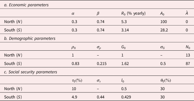
Assume first that a period spreads over 30 years. Supposing individuals enter the job market at 20 and, following the demographic features of 2010, we set ρ N = 1 in the North, which corresponds to a 60-year lifespan at 20 [United Nations (2017)]. Thereafter, as life expectancy at 20 is nearly 53 years in the South, we set (1 + ρ S,0)/2 = 53/60, then ρ S,0 = 0.764. From the United Nations (2017), the share of the world population aged between 20 and 49 in the South was 87% in 2010. Accordingly, at the initial period, we set N N,0 = 13 and N S,0 = 87. In addition, the share of the world population aged between 20 and 49 in the South was 80% in 1980, i.e., N S,−1/(N S,−1 + N N,−1) = 0.8. Fixing from the beginning a stable population in the North, i.e., G N = 1, the relative increase in the young population in the South as compared to the North gives the following equation:

With N N,0 = 13 and N S,0 = 87, this then leads to G S,0 = 1.62. With these values, the structure of the world population is satisfyingly reproduced for the first period of the model (2010) as exhibited in Table 1.
Calibration of the demographic transition: South's share of the world population

To characterize the demographic transition in the South, we assume that both its mortality and fertility rates converge toward the stationary levels prevailing in the North, which is supposed to have already completed its transition. Here, G S,t corresponds to half the fertility rate (net of child mortality), and 1 + ρ S,t is life expectancy at 20. The increased life expectancy in the South is then described by $\rho _{S,t}/\rho _{S,t-1} = \rho _{S,t-1}^{\sigma _\rho}$ and the decrease in its fertility rate evolves as follows: $G_{S,t}/G_{S,t-1} = G_{S,t-1}^{\sigma _G}$
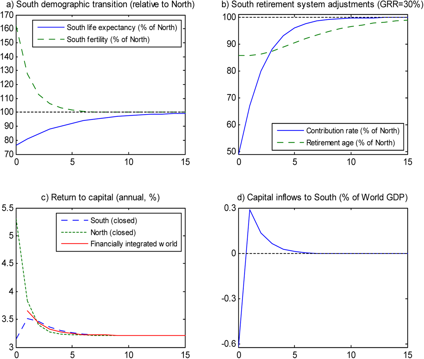
 for t ≥ 1, σ ρ and σ G denoting respectively the speed convergence of life expectancy and fertility toward a stable population. Note that if these speeds are nil, there is no demographic transition, whereas the transition ends after one period if they are equal to one. Speed σ G is chosen to reproduce the share of the world population aged between 20 and 49 in the South as forecast by the United Nations (2017) for 2040, 2070, and 2100. The results described in Table 1 obtain with σ G = 0.5, which characterizes a fast convergence toward the steady-state fertility level, that is, two children per woman. We then set σ ρ = 0.215 to account for the share of the world population over 20 in the South, which reflects a lower mortality convergence speed than the one prevailing for fertility. The respective evolutions of the fertility rate and life expectancy in the South are given in Figure 2a. Using this simple method to evaluate the structure of the world population after 2100 leads to the stabilization of the share of the world population over 20 in the South at 91.6%.
The benchmark scenario.

Besides, we assume a 0.99 annual discount time factor, so that β = 0.9930 ≈ 0.74 (Table 2). As usual, we set capital's share in output to α = 0.3. Put under pressure by population aging, social security in the South must adjust. Different options are available: postponing the legal retirement age, raising the pension contribution rate, reducing the pension benefits, or any combination of the three. As suggested in Figure 1-b3, pension benefits from 2010 should stabilize at a gross replacement rate $\theta _S = 30\%$ . In addition, even if stabilization in the North takes place a little later than in the South, the same level of pension indexing ($\theta _N = 30\%$
 ) also appears relevant for the former. For these reasons, we assume for both regions a permanent 30% gross replacement rate. Assuming the legal retirement age is 65 in the North, i.e., l N = 0.5, the required contribution rate τ N for a balanced budget [equation (4)] is then about 10% (against 11.7% actually observed in 2010). In the South, in the first period, as the social security size is 49% of the North's (Figure 1-b2), i.e., $\tau _{S,0} = 4.9\%$
 , the legal retirement age allowing pension benefits to be financed with a balanced budget corresponds to a little less than 63 years, or l S,0 = 0.429. We set the TFP in the North A N = 100 as the technological leader. To mimic the near 25% South-to-North ratio of GDP per capita (see Appendix A), we set A S = 28.2. Moreover, this benchmark scenario considers that there is neither technological innovation in the North nor technological convergence of the South with the North: $\hat{A}_N = \hat{A}_S = 0$
 .
Calibration

Assuming a 30% gross replacement rate in the South implies that the required adjustments in its retirement system consist in delaying the legal retirement age or raising the contribution rate. From Figure 1-b2, the relative size of the pension scheme in the South is expected to increase from 49% in 2010 to 68% in 2040. From that perspective, we assume that the contribution rate converges with the North's, according to an exogenous dynamics described by $\tau _{S,t}/\tau _{S,t-1} = \lpar {\tau_N/\tau_{S,t-1}} \rpar ^{\sigma _\tau}$ , σ τ denoting the speed of institutional convergence. This leads to σ τ = 0.44. Thereafter, the legal retirement age in the South will be supposed to adjust endogenously to maintain both a balanced budget and an unchanged gross replacement rate $\lpar {\theta_{t,S} = 30\%, {\rm \; for\; all\;} t} \rpar$
 . The corresponding evolutions of the contribution rate and the legal retirement age are given in Figure 2b.
Finally, assuming the return to capital (before tax) calculated by Piketty (Reference Piketty2013) for the period 1950–2012 is characteristic of the North's, we set $R_{N,0} = 5.3\%$ . Also, we set the risk-free return to capital in the South at $R_{S,0} = 3.14\%$
 so as to reproduce a net capital outflow in the South amounting to 0.62% of world GDP in 2010 (9-year moving average centered on 2010), as specified in the introduction.
In our simulation, reflecting the Lucas Paradox in line with Gourinchas and Jeanne (Reference Gourinchas and Jeanne2013) and Wang et al. (Reference Wang, Wen and Xu2015), a positive capital flowing from the South to the North is observed in period 0 because, one period after opening, the (equivalent) closed-economy risk-free interest rate in the North is still higher than in the South (Proposition 2). These upstream capital flows contribute to explain the fall in the interest rate observed over the past 25 years in the industrial world [see Eggertsson et al. (Reference Eggertsson, Mehrotra and Robbins2019)]. This global imbalance does not last, due to the swap of the relative positions of the two closed-economy interest rates. In effect, from the second period on, capital flows are directed from the North to the South (Figure 2d). However, the benchmark scenario evidences that the interest rate should go on decreasing due to the fast aging of the South population. Afterward, these positive flows in percentage of world GDP are decreasing and become insignificant after period 7.
As a matter of fact, with the population in the South converging toward a similar demographic structure as the North's, and the same trend prevailing for pension schemes, both closed-economies converge toward the same interest rate. As exhibited by equation

characterizing the closed-economy interest rate at steady state, the different TFP levels in the two regions (A S and A N) do not imply that their interest rates differ. As put forward by Proposition 2, capital flows then dry up.
3.2 The specific effects of the reduction in fertility
To study the specific effects of the reduction in fertility, we now compare the benchmark scenario with one assuming an unchanged fertility.
The effects of the drop in fertility G S,t in the South are unveiled primarily through the induced decline in its labor force growth leading to a decrease in both capital productivity and demand for capital. This results in a twofold decrease in the world interest rate (Figure 3a) and in capital inflows to South (Figure 3c).
The specific effects of fertility decline in the South depending on the retirement system adjustment (GRR = 30%).

Note that when capital flows are evaluated in percentage of world GDP as in Figure 3c, the fertility reduction seems to have no effect on them at steady state. On the one hand, as already described in the benchmark scenario, the convergence of population and social security structures equalizes the equivalent closed-economy regional interest rates, thus ending capital flows (Proposition 2). On the other hand, when the South population goes on growing forever, the world demographic share of the North becomes negligible and world GDP tends to infinity. Hence, the capital flows expressed as a share of world GDP tend to zero. Also, as the world interest rate decreases, the saving rates in the South and in the North are shown to decrease (Figure 3b).
As exhibited in Figure 3, the effects of the drop in fertility G S,t in the South must also be analyzed through the decline in the ratio of contributors (workers) to beneficiaries (retirees), that is, the dependency ratio (ρ S,t − l S,t)/(G S,t + l S,t). Induced aging puts pressure on pension systems to adjust. Maintaining the replacement rate θ S,t at 30%, where θ S,t = ((G S,t + l S,t)/(ρ S,t − l S,t))τ S,t, then requires, everything else being equal, either a progressive increase up to 3 percentage points in the retirement contribution rate τ i,t (Figure 3, left column) or a progressive increase up to 15 percentage points in the working period l S,t (Figure 3, right column). The increase in the contribution rate reduces workers' disposable income, which in turn contributes to reducing their savings to maintain their level of consumption when young. This fall in the saving rate is however insufficient to offset the decline in the investment rate as the capital inflow expressed as a share of world GDP decreases. Lengthening the working period also contributes to reducing the need for savings, thanks to a reduction in the period of life without income from work when old. In addition, this longer working period has a positive impact on the size of the labor force, which reduces the decline in the return to capital as compared to a contribution increase. However, this increase is insufficient to offset the decrease in the number of new workers. Similarly, the drop in savings is not enough to offset the effect of the decline in capital demand in the South. As a consequence, the world interest rate decreases. In the end, the Southern economy is always less dependent on incoming capital flows, regardless of the way its retirement system is adjusted.
Finally, from the second period (t = 1) onward, reducing the capital flowing to the South positively impacts the North, despite the decline in the interest rate. A smaller world population makes it possible to produce and consume more (Figure 3d). This is especially true in the South when the choice is made to work longer. In this case, the average consumption level increases by 6% at steady state. Conversely, when the adjustment of the pension schemes is done through the level of contribution, consumption increases by only 4% at steady state, and even decreases a little during the first two periods (this reflects the sharp fall in the interest rate during these periods).
3.3 The specific effects of the mortality reduction
Similarly to what has just been examined for fertility, we study the specific effects of a mortality reduction by comparing the benchmark scenario with one assuming an unchanged mortality.
The impact of the drop in mortality is twofold. First, as described before, it has a direct impact on savings behavior in the South: with a constant lifecycle income, living longer requires greater savings. Second, the increased number of retirees as compared to workers requires an adjustment of the pension system to comply with the permanent 30% replacement rate. In the case where the adjustment rests on higher contributions (Figure 4, left column), the contribution rate increases progressively to reach 15 percentage points as compared to the scenario with no mortality decline. Disposable income is then reduced, though not enough to offset the increased savings needs: people in the South save more with an unchanged labor force. Besides, on the world capital market, as the supply of capital increases, the interest rate declines progressively to reach −0.25 percentage point. In return, people in the North save less. Obviously capital flows to the South shrink, by 0.2 percentage point first, then progressively by 0.45 percentage point as mortality goes on declining in the South to reach the North's level. The gain in longevity in the South benefits the North since more capital per worker is available, which boosts consumption up to 1.5% at steady state.
The specific effects of mortality decline in the South depending on the retirement system adjustment (GRR = 30%).

On the other hand, consider that the retirement system adjustment is based on an increase in the working period, which would progressively reach 17 percentage points (Figure 4, right column). So, the increase in the South labor force makes the capital more profitable and generates an additional demand for capital with respect to what prevails in the contribution adjustment case. As evidenced by our simulation, the additional supply of capital in the South induced by increased longevity is completely offset by the additional demand for capital in the South, so that the world interest rate remains unchanged. Note that the very weak change in the saving rate observed in the South (Figure 4b, right column) implies that individual savings evolve proportionally to GDP:

Accordingly, the capital flows as well as consumption in the North remain unchanged as compared to the scenario with fixed mortality. From that perspective, an adjustment in the South retirement system through an increase in the pension contribution rates would benefit the North more than would an adjustment through the legal retirement age, although with only a small gain (1.5% at steady state). As the working period lengthens in the South, the increase in consumption over the life-cycle is about 30% stronger at steady state, as compared to 25% stronger in case of a pure contribution adjustment (Figure 4d). Interestingly enough, the lengthening of the working period allows the annual consumption flow to stay put. This means that consumption over the life-cycle increases by 30% at steady state due to the fact that life expectancy increases by 30%. Also, if the retirement system is adjusted through higher pension contributions, the annual consumption flow decreases by 5% at steady state.
4. Technological catching-up and capital flows: a robustness analysis
Previous simulations were made by assuming no technological catching-up of the South with the North. As a consequence, as observed in Figure 5, the South's GDP per capita expressed relatively to the North's, specified byFootnote 6

where ∂Γt/∂G S,t ≥ 0, ∂Γt/∂ρ S,t ≤ 0, and ∂Γt/∂l S,t ≥ 0, decreases after opening. After peaking in 2010 at 25%, it re-reaches its former level as observed between 1960 and 2000, at around 18%, based on the population over 20 (see Appendix A). This is due to the simultaneous decrease in fertility G S and increase in longevity ρ s, whereas the increase in the South working period l S is not sufficient to offset the demographic trend.
South's technological catch-up: past and forthcoming evolutions.

Contrasting to such a perspective, studies from Maddison (Reference Maddison2008) and Wang et al. (Reference Wang, Medianu and Whalley2011) tend to support that the South–North wealth gap will continue to narrow as observed since the beginning of the 21st century. In our setting, as underlined by equation (17), this narrowing requires a technological catching-up of the South with the North. Though our paper does not focus on the South's technological catch-up, it is worth testing our results for robustness by considering different scenarios for the convergence speed.
To that effect, the South's technological catch-up is modeled according to the following process: $A_{S,t}/A_{S,t-1} = \lpar {A_N/A_{S,t-1}} \rpar ^{\sigma _A}$ for t ≥ 1 with σ A < 1, where σ A measures the speed of technological convergence. In our previous benchmark scenario, σ A was set to zero to have no TFP growth in the South, i.e., $g_{A_S,t} = (A_{S,t}-A_{S,t-1})/A_{S,t-1} = 0$
 for all t ≥ 1. Now, we contemplate a fast technological catch-up (σ A = 0.45) which mimics the GDP per capita trends observed at the beginning of the 21st century (Figure 5b). In this new scenario, technological convergence is completed at the horizon of 2300 (period 10) and the TFP in the South stops growing. Finally, we investigate a slow technological catch-up scenario (σ A = 0.1) in which only half of the technological gap has been filled at the same horizon so that productivity continues to grow. As shown in Figure 6a, the TFP growth rate with slow convergence becomes greater than the one prevailing in case of fast convergence from period 5.Footnote 7 As to the curves of world interest rate associated to the two speeds of convergence, they exhibit similar shapes because their dynamics are linked to $g_{A_S,t}$
 through ΦS,t. The return to capital under fast convergence is greater than otherwise until the fifth period (Figure 6b).
The benchmark scenario: sensitivity to the speed of catching-up.

Considering the capital flow toward the South, the technological catch-up exerts two effects on the Southern economy. First, it increases its attractivity on the world capital market, which in turn pushes up the investment in the South. Second, the South's development due to catching-up increases the disposable income leading to higher households' savings. The world market financial tension is impacted by these two effects in opposite directions. However, the former effect dominates the latter: both world interest rate and capital flow toward the South increase with respect to a scenario without technological convergence (Figures 6b and 6c).
Let us now compare the impacts of the South's demographic transition under the three convergence scenarios. Figure 7 evidences the specific impacts of fertility and mortality declines on return to capital and capital flows. Thus, as illustrated in Figures 7a and 7c (left column for the latter), the interest rate drops caused by the fall in fertility or in mortality are all stronger in the first periods in case of fast technological catch-up.
Sensitivity of the effects of the South demographic transition to the technological catching-up speed.

Considering a fertility decline, the differences in the levels of impact are only temporary. Indeed, at steady state, if there is no convergence in fertility, the North economy becomes relatively negligible as compared to that of the South's (the share of world population in the South tends to 100%).
As for a decrease in mortality, we observe that the intensity of its impact differs, but this difference is permanent when the social security adjustment is exerted through the pension contribution rate: −0.26 percentage point without catching-up at steady state, −0.38 otherwise. Note that the fall in the interest rate is completely offset by the increase in the working period. This general result obtains whatever the speed of technological catch-up (Figure 7c, right column).
Turn now to the impact on capital flows (Figures 7b and 7d, left) when social security is adjusted through the contribution rate. Considering a fertility decline (Figure 7b, left), its impact deserves particular attention because the speed of technological catch-up matters qualitatively. The quicker the TFP growth, the weaker the relative variations of the saving and investment rates. Then, in the first periods, the decline in capital flows directed to the South is smaller the faster the catching-up. Afterward, we observe that the effect can be reversed in case of a slow technological convergence. To understand this effect, consider formally what is precisely depicted in the above figures referenced to:

We know from the convergence processes that KF S(G S → 1, A S → A N) → 0, and Y W(G S >1, A S → A N) → +∞. So both ratios tend to zero, but at potentially different speeds. If the former goes to zero more quickly than the latter, this measured difference stays negative through the whole process. Since fertility convergence in our calibration is assumed to be rapid, this is what prevails when there is no or fast technological catching-up. Conversely, the measured difference can become positive if the technological catch-up is slow.
Considering a mortality decline (Figures 7d, left), at steady state, the reduction in the capital flows goes from −0.47 percentage point with no catching-up to −0.16 point otherwise.
If the adjustment of the pension scheme is achieved through postponing the legal retirement age, the result obtained without catching-up remains consistent with technological catching-up: the additional supply of capital in the South generated by increased longevity is completely offset by the additional demand for capital in the South (Figure 7d, right column).
5. Conclusion
This paper develops a tractable two-period two-region OLG model. It permits a thorough analytical expression of the dynamics of the world interest rate and a clear exposition of the underlying interactions between the different regional components of world equilibrium. This contributes to a better understanding of the main mechanisms triggered by globalization. The advantages of our approach rooted in an analytical framework are twofold. First, tractability allows us to evidence clear-cut transitory dynamics. Second, it opens a path to possible investigations of general analytical properties of demographic changes.
Thus, we show that a declining fertility or increasing longevity may have an ambiguous impact on the direction of international capital flows. Although it triggers different mechanisms, the decline in mortality or fertility leads to similar effects, which result in a decrease in the need for capital. In the first case, the effect is induced mainly by an initial decline in the growth of the labor force. In the second case, a longer life increases incentives to save. Second, these initial changes may or may not be counterbalanced by the adjustment of pension schemes that can reduce or expand incentives to save or increase the labor force by delaying the legal retirement age, which in turn increases the investment demand. Finally, the decline in regional financial tensions affects the world interest rate, which in turn increases regional investment demands, which may increase the investment rate in the South.
To clear-up any ambiguity and to study the South's demographic transition, which involves a succession of shocks, the model is then calibrated on data characterizing the economies of the North and the South. The simulations show that the demographic transition tends, in a rather general way, to reduce the relative capital needs of the economies of the South. This, in turn, generates beneficial effects for the economies of the North, where the capital intensity and level of consumption are increased. The overall result depends on the choice of adjustment to guarantee the balance of the pension system. If delaying the legal retirement age is chosen to face an increased life expectancy, the relative capital needs to remain unchanged. Also, the results are sensitive to the development context. First, the magnitude of the initial impact of the demographic shock is reduced with catching-up. Second, over a finite horizon, in case of slow catching-up, the relative capital requirements in the South may also increase.
For future research, it is worth noting that the model has three main limitations. First, supposing an exogenous labor supply implies it is harmless in terms of welfare to delay the legal retirement age. In this perspective, this policy choice may appear misleadingly better than its alternative, an increase in contributions. Second, global heterogeneity bears only on the demographic and productive dimensions. To extend the long-run realism of the model, it would be wise to integrate other factors of production such as land or non-renewable resources. Finally, the perfect market equilibrium assumptions could be relaxed. For example, the model of Eggertsson and Mehrotra (Reference Eggertsson and Mehrotra2014) with rationed financial and labor markets, along with binding zero lower bound, opens up new research opportunities to study a global equilibrium with some economies potentially in secular stagnation and to see how an asynchronous demographic transition could explain some regional excess of savings and the very low rate of interest prevailing across many countries at the moment.
Acknowledgements
Without implication for any responsibility, we thank the co-editor and the reviewers of the journal for stimulating suggestions that have enabled us to significantly reformulate the paper's arguments and structure.
Appendix A: Data
A.1 Definition of the geographical areas North and South
A.1.1 Countries in the North (27 countries)
The countries belonging to the North are the following: Australia, Austria, Belgium, Canada, Switzerland, Czech Republic, Germany, Denmark, Spain, Finland, France, UK, Greece, Ireland, Iceland, Italy, Japan, Korea, Luxembourg, Netherlands, Norway, New Zealand, Portugal, Slovakia, Slovenia, Sweden, and USA.
Note that this definition of the North is similar to the one in Clements et al. (Reference Clements, Coady, Soto, Eich, Kangur, Kapsoli, Kashiwase, Nozaki, Shang and Thakoor2011).
A.1.2 Countries in the South (170 countries)
The countries belonging to the South are all the countries of the World (197 countries, United Nations) minus those belonging to the North (27 countries).
A.1.3 Sources
Demographic data: World Population Prospect. The 2015 Revision [United Nations (2017)] and authors' calculations.
First, we compute the population by age group j in each region (I = N, S) at date t as: ${\rm Po}{\rm p}_{I,j,t} = \mathop \sum \nolimits_{i\in I}{\rm Po}{\rm p}_{i,j,t}$ , where Popi,j,t denotes the population by age group (of 5 years) in country i at date t from the World Population Prospect. Note that, after 2015, we use the data from the medium variant. Then, we can calculate the total population in each region at date t, ${\rm Pop}T_{I,t} = \mathop \sum \nolimits_j{\rm Po}{\rm p}_{I,j,t}$
 , the population over age 20, ${\rm Po}{\rm p}_{I,20,t} = \mathop \sum \nolimits_{j \ge 20}{\rm Po}{\rm p}_{I,j,t}$
 , and the demographic dependency ratio as

The population growth at date t as given in Figure 1-a2 is then obtained by

and the demographic dependency ratio of the South to the North as given in Figure 1-a3 by

We also calculate the life expectancy LEI,j,t at age j and the fertility rate TFRI,t in each region I at each date t. By simplicity, these are calculated in proportion to the populations:

and

where LEI,j,t and TFRI,t denote respectively the life expectancy at age j and the total fertility rate in country i at date t in the United Nations' (2017) World Population Prospects. Figure 1-a1 depicts then the evolution of the relative life expectancy at birth in the South compared to the North, LES,0,t/LEN,0,t × 100, and likewise for the relative fertility rate in the South: TFRS,0,t/TFRN,0,t × 100.
GDP per capita data: Penn World Table, version 9.0 [Feenstra et al. (Reference Feenstra, Inklaar and Timmer2015)], and authors' calculations.
From the Penn World Table we compute the GDP per capita YpcI,t(PWT) in each region at each date t according to:

where Y i,t(PWT) denotes the real GDP and PopT i,t(PWT) the total population in country i at date t. Then, we construct data in a 9-year moving average ${\bar{\rm Y}p}{\rm h}_{I,t}\lpar {{\rm PWT}} \rpar$ , and we use our demographic data to establish the GDP per capita for the population over age 20: ${\rm Yp}{\rm c}_{I, + 20,t} = {\bar{\rm Y}p}{\rm h}_{I,t}\lpar {{\rm PWT}} \rpar ({\rm Po}{\rm p}_{I,t}/{\rm Po}{\rm p}_{I,20,t})$
 . Finally, as given in Figure 5, the relative GDP per capita in the South as compared to the North is Γt = (YpcS,+20,t/YpcN,+20,t) × 100.
Social security data: Clements et al. (Reference Clements, Coady, Soto, Eich, Kangur, Kapsoli, Kashiwase, Nozaki, Shang and Thakoor2011), and authors' calculations.
As our definition of the North is the same as Clements et al. (Reference Clements, Coady, Soto, Eich, Kangur, Kapsoli, Kashiwase, Nozaki, Shang and Thakoor2011), we can directly use their data on the size of the North retirement system as a percentage of GDP (Figure 1-b1). By contrast, as they focus only on emerging countries, we modify their data by incorporating the sub-Saharan countries. In 2010, the size of the retirement system amounted to $\gamma _{AfSS,2010} = 0.7\%$ of GDP in the latter [Marchiori (Reference Marchiori2011)]. Accordingly, as their GDP represents 6% of the GDP of the South (authors' calculations based on Penn World Table data) and as the size for the emerging countries calculated by Clements et al. is $\gamma _{{\rm Emerging},2010} = 4.2\%$
 , in 2010 we set that the social security size in the South is $\gamma _{S,2010} = 0.06 \times \gamma _{AfSS,2010} + 0.94 \times \gamma _{{\rm Emerging},2010} = 4.0\%$
 . Thereafter, as given in Figure 1-b1, we compute the evolution of the South social security size as: γ S,t = γ Emerging,t × (ΨS,2010/γ Emerging,2010). The relative evolution of the South social security size (Figure 1-b2) is then obtained at each date by γ S,t/γ N,t × 100.
To get the gross replacement rate in percentage of the last wages θ, as given in Figure 1-b3, we first assume a balanced budget, namely θ I,t = τ I,t/DR I,t, where DR I,t denotes the dependency ratio and τ i,t the pension contribution rate in each region I at each date t. Then, assuming that capital's share in output is α = 0.3, this implies that τ I,t = γ I,t/(1 − α) = γ I,t/0.7, and we assume that DR I,t = DDR I,t. Note that this method enables us to obtain in 2010 in the North a gross replacement rate equal to 43.2%. To compare with an alternate method, we have also calculated the gross replacement rate using the gross replacement rates provided by the OECD in proportion to the GDP of the Northern countries, and we obtain for the same year a rate equal to 42.2%.
Appendix B: Proofs of the propositions
B.1 Proposition 1
From equations (1), (8)–(12), and (15) we have:

From equation (11), it follows that the wage and the capital per worker depend on the world interest rate such that:

where

Introduction of equations (8) and (B.2) into equation (B.1) then yields:

Using equations (B.3) and (B.4), the dynamics of the world general equilibrium can be specified as:

where

This then yields straightforwardly that Φt can be rewritten as

or equivalently

where

and

B.2 Proposition 2
From equations (11), (8), and (B.3), in an economy with fully integrated capital markets both in period t and t + 1, this yields $KF_{i,t} = L_{i,t + 1}A_{i,t + 1}^{1/(1-\alpha )} {\bi k}\lpar {R_{t + 1}} \rpar -N_{i,t}{\bi S}_{i,t}\lpar {R_t,R_{t + 1}} \rpar$ , where ${\bi S}_{i,t}\lpar {R_t,R_{t + 1}} \rpar \equiv s_{i,t}\lpar {1-\tau_{i,t}} \rpar A_{i,t}^{1/(1-\alpha )} {\bi w}\lpar {R_t} \rpar -\lpar {1-s_{i,t}} \rpar b_{i,t + 1}((1-\alpha )/\alpha )A_{i,t + 1}^{1/(1-\alpha )} {\bi k}\lpar {R_{t + 1}} \rpar$
 .
By contrast, in an economy open in t but in autarky in t + 1, it yields $L_{i,t + 1}A_{i,t + 1}^{1/(1-\alpha )} {\bi k}\lpar {{{\tilde R}}_{i,t + 1}} \rpar = N_{i,t}S_i\lpar {R_t,{{\tilde R}}_{i,t + 1}} \rpar$ .
We deduce that the capital flow in region i and in period t can be rewritten as:

As k (.) is a decreasing function of the interest factor, we conclude that:

Appendix C: Sensitivity of the world capital allocation to demographic changes: the case of non-permanent anticipated shocks
The demographic shocks directly impact the population size (consumers, workers, and retirees) and the life-cycle saving tradeoff. They also convey many indirect effects through the institutional adjustment of pension systems and price changes on the domestic and international markets.
To analyze their impacts on the world capital allocation at a regional level, it is worth decomposing the effects transiting through either the demand for capital, i.e., the investment, or its supply, i.e., the savings, in each region. To that end, denote by invri,t = K i,t+1/Y i,t, i = N, S, the macroeconomic investment rate in region i and in period t. As k i,t+1 = K i,t+1/L i,t+1, it follows according to equations (1), (12), and (B.2) that the investment rate can be rewritten as

Using equations (16) and (B.3), this also yields

Accordingly, this rate can be rewritten as ${\rm inv}{\rm r}_{i,t} = (G_{i,t}/(G_{i,t} + l_{i,t})) \; \widetilde{{{\rm invr}}}_{i,t}$ where the multiplier G i,t/(G i,t + l i,t) is the share of young workers in the total labor force and

denotes the investment rate per young worker as a percentage of the added value per worker.
Similarly, denote by savri,t = (N i,tS i,t)/Y i,t the macroeconomic saving rate. From equations (1), (8), (12), and (B.2), this yields

The use of equations (16) and (B.3) allows us to rewrite the saving rate as

It can also be rewritten as ${\rm sav}{\rm r}_{i,t} = (G_{i,t}/(G_{i,t} + l_{i,t}))\widetilde{{{\rm savr}}}_{i,t}$ , where $\widetilde{{{\rm savr}}}_{i,t}$
 is the saving rate expressed in percentage of the added value per worker:

The net capital inflow in a region i being defined as the difference between the demand and the supply of capital, i.e., KF i,t = (invri,t − savri,t)Y i,t, we can then express the ratio KFr i,t = KF i,t/Y i,t as:

Accordingly, the impact of the demographic changes on the international capital flows can be split into three expressions:

where

The two components of the first expression measure the impact on the investment and savings behaviors, expressed as a proportion of the added value per worker, assuming a constant tension on the world capital market (ΔΦt = 0). The following expression measures the change in the young workers' share in the labor force. As a whole, these two expressions result in a global impact, denoted ${\Delta KFr_{i,t}} \vert _{\Delta \Phi _t = 0}$ , characterizing a small open economy. Indeed, as $R_{t + 1} = R_t^\alpha \Phi _t^{1-\alpha}$
 , considering ΔΦt = 0 is equivalent to assuming a constant interest rate in period t + 1, i.e., ΔR t+1 = 0. The last expression measures the intensity of the feedback effect induced by the changes in the demand and supply of capital in the world capital market. It depends on the variation of the tension indicator Φt. ΔΦt > 0 (resp. < 0) means a higher (resp. lower) financial tension, inducing a decrease (resp. an increase) in the capital-to-labor ratio. The variation of Φt captures the international spillover effects of a demographic change.
Note that $\widetilde{{{\rm invr}}}_{i,t}-\widetilde{{{\rm savr}}}_{i,t}$ can be either positive or negative. However, for reasonable parameters, it appears that ΦS,t+j − ΦN,t+j is positive for all j >1 (see section 3) so that, from Proposition 2, we can infer that capital flows from the North to the South. Accordingly, the following assumption applies:

C.1 Negative fertility shock
Consider a negative non-permanent shock in fertility rate in the South in period t + 1, ΔG S,t+1 < 0, anticipated in period t. Before investigating its impact on the international capital flows, it is crucial to underline that this shock requires in period t + 1 a social security adjustment, because it means fewer workers pay for the pension benefits. From equation (10), ΔG S,t+1 < 0 implies in period t + 1 a social security adjustment (SSA) through either:
(1) a pension contribution increase:
(C.5)$$\Delta \tau _{S,t + 1} = -\displaystyle{{\tau _{S,t + 1}} \over {G_{S,t + 1} + l_{S,t + 1}}}\Delta G_{S,t + 1} \gt 0,$$
(2) or a pension reduction:
(C.6)$$ \hskip-1.4pc\Delta \theta _{S,t + 1} = \displaystyle{{\tau _{S,t + 1}} \over {\rho _{_{S,t + 1}} -l_{_{S,t + 1}}}} \Delta G_{S,t + 1} \lt 0,$$(3) or the postponing of the legal retirement age:
(C.7)$$\Delta l_{S,t + 1} = -\displaystyle{{\tau _{S,t + 1}} \over {\tau _{S,t + 1} + \theta _{S,t + 1}}}\Delta G_{S,t + 1} \gt 0.$$


Considering these various possibilities, to disentangle the different channels through which the fertility shock in the South impacts the South and the North, we consider in a first step the South as a small economy by assuming ΔΦt = 0. In that case, the shock is supposed to have no effect on the North. In a second step, we consider the feedback effects induced by the changes in the demand and supply of capital in the world capital market that affect both the South and the North. We then review the capital accumulation at the global level.
C.1.1 The South as a small open economy
As specified in equation (C.4), capital flows in the South are impacted through the change in its investment, its savings or its young workers' share.
C.1.1.1 Mathematics
(a)
$$ {\Delta {\widetilde{{{\rm invr}}}}_{S,t + j}} \vert _{\Delta \Phi _{t + j} \,=\, 0}\fleqno$$

From equation (C.1), this yields in period t:

With the first two SSAs [equations (C.5) and (C.6)], it follows that:

With the third SSA [equation (C.7)], it is worth noting that the working population increases, but not enough to offset the initial effect:

Therefore, from equation (C.1), it follows that:

For other periods t + j, j ≥ 1:

(b)
$${\Delta {\widetilde{{{\rm savr}}}}_{S,t + j}} \vert _{\Delta \Phi _{t + j} = 0}\fleqno$$

From equation (C.2), it yields in period t:

where from equations (7) and (10) b i,t+1 = l i,t+1 + G i,t+1τ i,t+1 and then:
• with equation (C.5)
$$\hskip-3pc\eqalign{\Delta b_{S,t + 1} & = \tau _{S,t + 1}\Delta G_{S,t + 1} + G_{S,t + 1}\Delta \tau _{S,t + 1} \cr & = \tau _{S,t + 1}\left( {1-\displaystyle{{G_{S,t + 1}} \over {G_{S,t + 1} + l_{S,t + 1}}}} \right)\Delta G_{S,t + 1} \lt 0,}$$• with equation (C.6) Δb S,t+1 = τ S,t+1ΔG S,t+1 < 0,
• with equation (C.7)
$$\Delta b_{S,t + 1} = \Delta l_{i,t + 1} + \tau _{S,t + 1}\Delta G_{S,t + 1} = \tau _{S,t + 1}\left[ {\displaystyle{{\theta_{S,t + 1}-\lpar {1-\tau_{S,t + 1}} \rpar } \over {\tau_{S,t + 1} + \theta_{S,t + 1}}}} \right]\Delta G_{S,t + 1}.$$


In that case,

The first two SSAs [equations (C.5) and (C.6)] reduce households' expected future income when old, yielding the current saving rate to increase:

The impact of the third SSA [equation (C.7)] depends on the gap between the net wage and pension, a function of (1 − τ S,t+1) − θ S,t+1, or the pension net replacement rate, defined by θ S,t+1/(1 − τ S,t+1).
From equation (C.2), this yields in period t + 1:

and then according to equations (C.5)–(C.7):

In period t + j, j >1, equation (C.2) yields:

(c)
$$\hskip-26pc\Delta \displaystyle{{G_{S,t + j}} \over {G_{S,t + j} + l_{S,t + j}}}$$


The fertility drop reduces the share of the young workers in period t + 1 but not in periods t and t + j for j >1:

If the social security adjustment consists in postponing the legal retirement age [equation (C.7)], the reduction in t + 1 is amplified.
C.1.1.2 Analysis
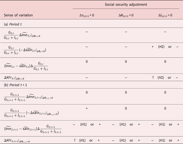
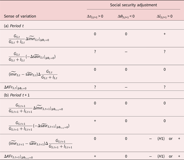
Table C.1 summarizes the domestic effects for the current (t) and next (t + 1) periods when the world financial tension is supposed unchanged (small open economy). In the South, the negative fertility shock in t results first in a reduction in the labor force of the next period, even if the retirement age is postponed as specified in the third social security adjustment. As a consequence, whatever the social security adjustment, the marginal productivity of capital is reduced in t + 1, which explains the investment rate decline in period t: $\Delta \widetilde{{{\rm invr}}}_{S,t} \lt 0$ . As the fertility rate returns to its initial level in period t + 2, the shock has no effect on the investment rate from the period t + 1 onward: $\Delta \widetilde{{{\rm invr}}}_{S,t + j} = 0,\;j \ge 1$
 .
Negative fertility shock in t + 1 (ΔG S,t+1 < 0): South domestic impact (small open economy)

As to the saving rate, it must be noted that individual income is affected differently by the negative fertility shock depending on the social security adjustment. Indeed, if the social security adjustment does not entail a lengthening of the working period in t + 1, the fertility shock in period t results in a lower income when old in t + 1: ${\Delta b_{S,t + 1}} \vert _{\Delta \Phi _t = 0,\Delta l_{S,t + 1} = 0} \lt 0$ . As a result, the current saving rate increases: ${\Delta {\widetilde{{{\rm savr}}}}_{S,t}} \vert _{\Delta \Phi _t = 0,\Delta l_{S,t + 1} = 0} \gt 0$
 . On the other hand, the impact of the third adjustment depends on the gap between the net wage and pension, tied to (1 − τ S,t+1) − θ S,t+1. If the pension net replacement rate, defined by θ S,t+1/(1 − τ S,t+1), is greater (resp. lesser) than 1, the saving rate is increased (resp. decreased). For reasonable parameters (see section 3) it appears that this ratio is less than 1, hence we assume:

so that ${\Delta {\widetilde{{{\rm savr}}}}_{S,t}} \vert _{\Delta \Phi _t = 0,\Delta l_{S,t + 1} \gt 0} \lt 0$ . Considering the next period saving rate, the adjustment through the pension contribution rate reduces the net wage of future young workers, which in turn leads to a contraction of the future saving rate ${\Delta {\widetilde{{{\rm savr}}}}_{S,t + 1}} \vert _{\Delta \Phi _{t + 1} = 0,\Delta \tau _{S,t + 1} \gt 0} \lt 0$
 . In the other cases, the fertility shock has no impact on the saving rate: ${\Delta {\widetilde{{{\rm savr}}}}_{S,t + 1}} \vert _{\Delta \Phi _{t + 1} = 0,\Delta \tau _{S,t + 1} = 0} = 0$
 . Note that, in case the future fertility shock is unexpected, only this saving impact will occur.
Finally, the fertility drop reduces the share of the young workers in period t + 1 (Δ(G S,t+1/(G S,t+1 + l S,t+1)) < 0) but not in periods t + j for j ≠ 1. This reduction is amplified if the legal retirement age is postponed. Assuming by H1 that $\widetilde{{{\rm invr}}}_{S,t + j}-\widetilde{{{\rm savr}}}_{S,t + j} \gt 0$ , it then yields

According to assumptions H1 and H2, the net result measured by ${\Delta KFr_{S,t + j}} \vert _{\Delta \Phi _{t + j} = 0}$ is clear-cut in most of the cases and highlights the decline in capital flows entering the South as a result of declining fertility. However, when the legal retirement age is postponed and when the contribution rate is increased the net impact is indeterminate in periods t and t + 1 respectively.
C.1.2 The spillover effects and the North
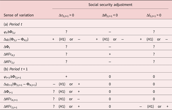
The above small open economy hypothesis goes with the assumption that the South demo-economic weight is insignificant, i.e., φ t+j ≈ 0. In that case, as Φt = φ tΦS,t + (1 − φ t)ΦN,t, a change in the South financial tension entails no significant change at the world market level: ΔΦt+j ≈ 0 even if ΔΦS,t+j ≠ 0. Relaxing the small open economy hypothesis requires then to take into account the impact of the fertility shock on the world financial market. As specified by the following equation, this impact decomposes into two distinct effects:

The first term measures the change in financial tension in the South, while the second term measures the change in the South demo-economic weight.
C.1.2.1 Mathematics
(a) ΔΦS,t+j
In period t,

and it follows that:

where


Accordingly:
• with equation (C.6),
$$\hskip-21pc\Delta \Phi _{S,t} = \displaystyle{{\partial \Phi _{S,t}} \over {\partial G_{S,t + 1}}}\Delta G_{S,t + 1} \lt 0,$$• with equation (C.5),
$$\eqalign{\Delta \Phi _{S,t} & = \displaystyle{{\partial \Phi _{S,t}} \over {\partial G_{S,t + 1}}}\Delta G_{S,t + 1} + \displaystyle{{\partial \Phi _{S,t}} \over {\partial \tau _{S,t + 1}}}\Delta \tau _{S,t + 1} \cr & = \displaystyle{{ [ {\alpha + \lpar {1-\alpha} \rpar \lpar {1-s_{S,t}} \rpar \tau_{S,t + 1}\lpar {1-(G_{S,t + 1}/(G_{S,t + 1} + l_{S,t + 1}))} \rpar } ] {\lpar {A_{S,t + 1}/A_{S,t}} \rpar }^{1/(1-\alpha )}} \over {s_{S,t}\lpar {1-\tau_{S,t}} \rpar \lpar {1-\alpha} \rpar }}\Delta G_{S,t + 1} \lt 0,}$$• with equation (C.7),
$$\eqalign{\Delta \Phi _{S,t} & = \displaystyle{{\partial \Phi _{S,t}} \over {\partial G_{S,t + 1}}}\Delta G_{S,t + 1} + \displaystyle{{\partial \Phi _{S,t}} \over {\partial l_{S,t + 1}}}\Delta l_{S,t + 1} \cr & = {\displaystyle{\matrix{{\lpar [ \alpha (\theta_{S,t + 1}/(\tau_{S,t + 1} + \theta_{S,t + 1})) + \lpar {1-\alpha} \rpar \lpar {1-s_{S,t}} \rpar (\tau_{S,t + 1}/(\tau_{S,t + 1} + \theta_{S,t + 1}))}\cr{{[ \theta_{S,t + 1}-\lpar {1-\tau_{S,t + 1} \rpar} ] } ]} \rpar {\lpar {A_{S,t + 1}/A_{S,t}} \rpar }^{1/(1-\alpha )}} \over {s_{S,t}\lpar {1-\tau_{S,t}} \rpar \lpar {1-\alpha} \rpar }}\Delta G_{S,t + 1} \gt 0.} $$


In this case,

Note that, by defining X = (G S,t+1 + l S,t+1)(A S,t+1/A S,t)1/(1−α)α, Y = s S,t(1 − τ S,t)(1 − α), Z = (1 − s S,t)b S,t+1(A S,t+1/A S,t)1/(1−α)(1 − α), we can rewrite $\widetilde{{{\rm invr}}}_{i,t} = (X/\Phi _t)$ and $\widetilde{{{\rm savr}}}_{i,t} = Y-(Z/\Phi _t)$
 , and it follows that:

On the other hand, ΦS,t = (X + Z)/Y and then

As ΔY = 0, we can verify in period t that $\Delta \Phi _{S,t} = (\Phi _t/Y) {\lpar {\Delta {\widetilde{{{\rm invr}}}}_{S,t}-\Delta {\widetilde{{{\rm savr}}}}_{S,t}} \rpar } \vert _{\Delta \Phi _t = 0}$ .
In period t + 1,

which yields:

where

In period t + j for j >1, ΔΦS,t+j = 0.
(b) Δφ t+j(ΦS,t+j − ΦN,t+j)
As

we can infer that in period t the South demo-economic weight does not change:

Otherwise, differentiating φ t+j in period t + 1 yields:

and for all the other periods t + j for j >1:

To determine the sense of variation of φ t+j for j ≥ 1, we derive first

or equivalently:

Second,

or:

Besides, as $\lambda _{S,t + j} = N_{S,t + j}/\sum _iN_{i,t + j}$ , it follows that

or equivalently:

From equation (1), $N_{S,t + j} = \mathop \prod \nolimits_{k = 1}^j G_{S,t + k}N_{S,t}$ yields $\log N_{S,t + j} = \mathop \sum \nolimits_{k = 1}^j \log G_{S,t + k} + \log N_{S,t}$
 and:

To summarize, this then yields that:

and then that:

C.1.2.2 Analysis
In period t, the changes in the tension in South domestic capital demand can be derived from the previous analyses. Indeed, it can be shown that

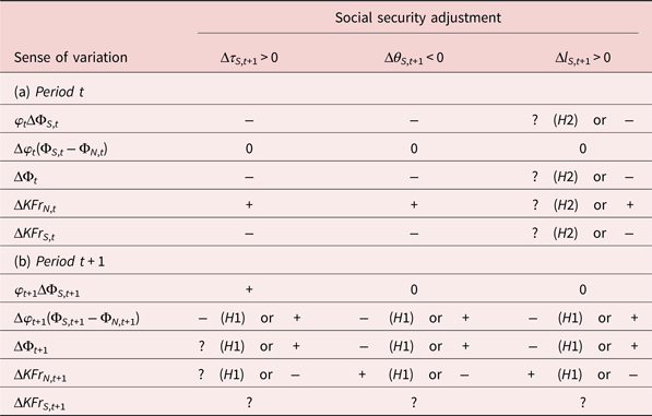
Since, as long as the retirement age stays put, financial tension in the South is decreased by the negative fertility shock: ${\Delta \Phi_{S,t}} \vert _{\Delta l_{S,t + 1} = 0} \lt 0$ . As described in Table C.1, either increased contributions or decreased pensions lead to both a lower investment rate and a higher saving rate. By contrast, a delayed retirement age, under assumption H2, decreases the saving rate, and the change in the South domestic tension is now indeterminate. In the period immediately preceding the shock, the South demo-economic weight is not impacted: Δφ t = 0. As highlighted in Table C.2, the global effect in period t is then expressed solely by the change in the South financial tension ΦS,t.
Conversely, in period t + 1, unless the social security adjustment is operated through the contribution rate, the financial tension in the South is no longer impacted by the fertility shock: ${\Delta \Phi_{S,t + 1}} \vert _{\Delta \tau _{S,t + 1} = 0} = 0$ . Only if the contribution rate increases does the saving rate decrease so that this tension grows: ${\Delta \Phi_{S,t + 1}} \vert _{\Delta \tau _{S,t + 1} \gt 0} \gt 0$
 . On the other hand, from period t + 1, the negative transitory fertility shock in the South will have a permanent negative effect on its population share in the world. The South demo-economic weight is then permanently impacted so that Δφ t+j < 0 for all j ≥ 1. Assuming a stronger tension in the South than in the North (H1) yields Δφ t+j(ΦS,t+j − ΦN,t+j) < 0. So, unless a social security adjustment goes with a higher contribution rate, financial tension at the world level is reduced in period t + 1 (see Table C.2).
Negative fertility shock in t + 1 (ΔG S,t+1 < 0): the spillover effects

Through the impact on tension on the world capital market, the fertility shock in the South spills over to the North such that, according to equation (C.4),

Therefore, when it is determinate and according to our assumptions, the negative fertility shock in the South in period t + 1, by entailing a lower world financial tension in periods t and t + 1 (see Table C.2), leads to

if ΔΦt+j < 0, for j = 0, 1.
C.1.3 Overall impact on the South and the world capital
By affecting the world interest rate, the spillover effects also bear consequences in the South, inducing an increase in its investment rate and a decrease in its saving rate when ΔΦt < 0. The overall effect on the South obtained from equation (C.4) is then indeterminate. To test whether the overall effect of the negative fertility shock on the relative South capital flows is truly indeterminate, one may also consider the following relation:

(as it is obvious that $\mathop \sum \nolimits_{i}KF_{i,t} = 0$ ) such that:

where

In period t, Δ(Y N,t/Y S,t) = 0 and it follows that

by assuming H1 (KFr S,t > 0 and KFr N,t < 0). We can deduce that in this period, the spillover effects conveyed through the variation of the interest rate reduce the effect acknowledged in the small open economy without altering its sense of variation: $\vert {\Delta KFr_{S,t}} \vert \lt \vert {{ {\Delta KFr_{S,t}} \vert }_{\Delta \Phi_t = 0}} \vert$ and ${\rm sign}\lpar {\Delta KFr_{S,t}} \rpar = {\rm sign}\lpar {{ {\Delta KFr_{S,t}} \vert }_{\Delta \Phi_t = 0}} \rpar$
 . This result depends on the channel through which the international financial tension is affected, i.e., a change in the South regional tension: ΔΦt = φ tΔΦS,t. However, by definition, if the South was in autarky, its domestic feedback would be measured by ΔΦS,t implying ΔKFr S,t = 0. This means that in the international context here considered, the spillover effects in the South are not sufficient to totally offset the small-open-economy effect: |ΔΦt| <|ΔΦS,t|.
Differently, in period t + 1, unless Δτ S,t+1 > 0, the South regional tension is unaffected, i.e., ΔΦS,t+1 = 0. Hence, the spillover effects do not depend on it but are still linked to the demo-economic weight of the South. As can be seen in equation (C.9),

where ΔKFr N,t+1/KFr N,t+1 < 0 if assuming H1 and Δτ S,t+1 = 0, whereas

(labor in the South is always decreased by the negative fertility shock, even if the legal retirement age is postponed). By a denominator effect, we can no longer assert that the capital flow-to-GDP ratio in the South systematically changes in the same direction as its counterpart in a small open economy. It is then indeterminate.
Note that in our simulations, in order to compare the capital flows from the different regions directly, we consider the flows with respect to the world GDP instead of the regional GDPs, such that

However, as

where

using this ratio does not help to clear-up the analytical indeterminacy evidenced in period t + 1 in the South.
C.2 Positive longevity shock
Consider now in period t + 1 a positive non-permanent shock in life expectancy in the South, Δρ S,t+1 > 0, anticipated in period t As this entails more pensioners, this shock requires a social security adjustment. From equation (10), Δρ S,t+1 > 0 implies in period t + 1 a social security adjustment through either:
(1) a pension contribution increase:
(C.10)$$\Delta \tau _{S,t + 1} = \displaystyle{{\tau _{S,t + 1}} \over {\rho _{S,t + 1}-l_{S,t + 1}}}\Delta \rho _{S,t + 1} \gt 0,$$(2) or a pension reduction:
(C.11)$$\Delta \theta _{S,t + 1} = -\displaystyle{{\theta _{S,t + 1}} \over {\rho _{S,t + 1}-l_{S,t + 1}}}\Delta \rho _{S,t + 1} \lt 0,$$(3) or the postponing of the legal retirement age:
(C.12)$$\Delta l_{S,t + 1} = \displaystyle{{\theta _{S,t + 1}} \over {\theta _{S,t + 1} + \tau _{S,t + 1}}}\Delta \rho _{S,t + 1} \gt 0.$$


To assess the impact of this shock, we proceed similarly as for the fertility shock. First, we consider the South as a small open economy. Then, we consider the feedback effects induced by the changes in the demand and supply of capital in the world capital market, and we finally review the changes in capital flows in the North and the South.
C.2.1 The South as a small open economy
C.2.1.1 Mathematics
(a) ${\Delta {\widetilde{{{\rm invr}}}}_{S,t + j}} \vert _{\Delta \Phi _{t + j} = 0}$

From equation (C.1), this yields:

With the first two SSAs [equations (C.10) and (C.11)], it follows that:

With the third SSA [equation (C.12)]:

(b) ${\Delta {\widetilde{{{\rm savr}}}}_{S,t + j}} \vert _{\Delta \Phi _{t + j} = 0}$

From equation (C.2), it follows in period t:

where

and b S,t+1 = l S,t+1 + G S,t+1τ S,t+1, and then:
• with equation (C.10), Δb S,t+1 = G S,t+1Δτ S,t+1 = G S,t+1(τ S,t+1/(ρ S,t+1 − l S,t+1))Δρ S,t+1 > 0
• with equation (C.11), Δb S,t+1 = 0,
• with equation (C.12), Δb S,t+1 = Δl S,t+1 = (θ S,t+1/(θ S,t+1 + τ S,t+1))Δρ S,t+1 > 0.
Accordingly, from equation (C.13) this yields:

In the other cases (Δτ S,t+1 > 0 or Δl S,t+1 > 0), the sign of $\Delta \widetilde{{{\rm savr}}}_{S,t}$ is indeterminate in period t.
From equation (C.2), it follows in period t + 1:

and then:

In period t + j, j >1:

(c) $\quad\Delta \displaystyle{{G_{S,t + j}} \over {G_{S,t + j} + l_{S,t + j}}}$

Differentiating

leads to

Then, increased longevity in t + 1 has no effect on the share of the young workers in period t + 1 unless the legal retirement age is postponed:

For the other periods t + j, j = 0 or j >1, the impact is nil.
C.2.1.2 Analysis
As exhibited by equation (8), for young domestic households in period t, the positive longevity shock that will occur in period t + 1 modifies in two ways their saving choice to sustain their consumption when old. First, it requires a higher saving effort (Δs S,t > 0). Second, as the future net income increases if social security is adjusted through the contribution rate or postponement of the legal retirement age (Δb S,t+1 > 0), it lowers the incentive to save. In these two cases, the responsiveness of savings is indeterminate in period t. In the last (third) case, the pension is reduced (Δθ S,t+1 < 0) but received for longer such that Δb S,t+1 = 0; only the first effect matters, and savings is then increased: ${\Delta {\widetilde{{{\rm savr}}}}_{S,t}} \vert _{\Delta \Phi _t = 0,\Delta \theta _{S,t + 1} \lt 0} \gt 0$ . As before, solely a contribution adjustment reduces the saving rate in period t + 1.
The positive longevity shock has no direct impact on the investment rate. Therefore, the latter upgrades only in period t if labor is increased through the postponement of the legal retirement age in period t + 1. Also, in this case, the young workers' share in period t + 1 is decreased, Δ(G S,t+1/(G S,t+1 + l S,t+1)) < 0, whereas it stays unchanged for the other periods t + j, j = 0 and j > 1.
Taking all these effects into account, as reported in Table C.3, it appears that the impact of the positive longevity shock in the South on the relative capital flow may be different, depending on the social security adjustment and the period. Hence, in period t, the effect is unambiguously negative only if pensions are reduced. In period t + 1, the impact is positive if the contribution rate is increased, negative (under H1) if the retirement age is postponed, or nil if pensions are decreased.
Positive longevity shock in t + 1 (Δρ S,t+1 > 0): South domestic impact (small open economy)

C.2.2 The spillover effects
The channels through which the world capital market is affected by the longevity shock in the South are the same as for the fertility shock, i.e., the changes in the domestic tension in the South ΔΦS,t and in its demo-economic weight Δφ t as specified in equation (C.8).
C.2.2.1 Mathematics
(a) ΔΦS,t+j
Differentiating

gives:

where ∂s S,t/∂ρ S,t+1 > 0, ∂ΦS,t/∂τ S,t+1 > 0, ∂ΦS,t/∂l S,t+1 > 0 (see the fertility shock) and

It follows that the sign of ΔΦS,t is only determinate if the SSA implies less pension benefits such that:

In period t + 1:

where ∂ΦS,t+1/∂τ S,t+1 > 0 (see the fertility shock).
(b) Δφ t+j(ΦS,t+j − ΦN,t+j)
In period t, differentiating

leads to:

where

and

In period t + 1, one gets:

where

It follows that:

In period t + j, j >1:

(c) ${\Delta \Phi_t} \vert _{\Delta \theta _{S,t + 1} \lt 0}$

Note that, in period t, as the result of indeterminate or opposing effects, the sense of variation of the spillover effect seems massively indeterminate. However, if considering the following specification

if pensions are lowered [equation (C.11)], and only in this case, the indeterminacy clears up such that the dominant effect is always brought through the South domestic tension:

C.2.2.2 Analysis
In period t, as the change in the saving rate is indeterminate if social security is adjusted through contributions or the legal retirement age, the change in the domestic tension in the South is also indeterminate. Only if the social security adjustment goes with less pension benefits, as savings hence capital supply are increased, do we know that the domestic tension is lowered in the South. In period t + 1, for the same reason as for the negative fertility shock, the domestic tension is impacted and increased only if the contribution rate is increased.
Contrary to the fertility shock, the South demo-economic weight is impacted and increased as early as period t by the positive longevity shock through the savings channel: Δφ t > 0. Under assumption H1, it follows that Δφ t(ΦS,t − ΦN,t) > 0. From period t + 1 on, unless the social security adjustment yields an increase in contributions characterized by

the demo-economic weight of the South is no longer affected by the longevity shock, ${\Delta \varphi_{t + 1}} \vert _{\Delta \tau _{S,t + 1} = 0} = \Delta \varphi _{t + j,\,j \gt 1} = 0$ , reflecting the transitory nature of a longevity shock on demographics, unlike a fertility shock.
Table C.4 summarizes the net effect of each impact for the current and next period. In period t, as the result of indeterminate or opposing effects, the sense of variation of the spillover effect may appear massively indeterminate. However, it can be shown that if pensions are lowered, the dominant effect always passes through the South domestic tension so that ${\Delta \Phi_t} \vert _{\Delta \theta _{S,t + 1} \lt 0} \lt 0$ . Only in this case can we assert, under H1, that the capital flows from the North to the South expressed relatively to North GDP decrease in period t: ${\Delta KFr_{N,t}} \vert _{\Delta \theta _{S,t + 1} \lt 0} \gt 0$
 . In period t + 1, if the social security adjustment does not entail a higher contribution rate, the world financial tension stays unchanged, as do the capital flows with respect to North GDP: ${\Delta \Phi_{t + 1}} \vert _{\Delta \tau _{S,t + 1} = 0} = {\Delta KFr_{N,t + 1}} \vert _{\Delta \tau _{S,t + 1} = 0} = 0$
 . In the opposite case, the variation of the world financial tension is indeterminate under H1.
Positive longevity shock in t + 1 (Δρ S,t+1 > 0): the spillover effect

C.2.3 Overall impact on the South
In period t, as for the fertility shock, the global effect of a positive longevity shock in the South can be obtained by equation (C.9). As labor in the South is not impacted, the change in the relative capital flows in the South is always of the opposite sign to the change in the relative capital flows in the North: ΔKFr S,t/KFr S,t = ΔKFr N,t/KFr N,t, where KFr S,t > 0 and KFr N,t < 0 according to H1.
In period t + 1, if the social security adjustment entails a higher contribution rate, the effect is globally indeterminate, both in the North, as already seen, and in the South. By contrast, otherwise, as there is no spillover effect, the global effect in the South is the same as the one prevailing in the small open economy, i.e., none if a social security adjustment entails less pension benefits, or less capital flows entering expressed relatively to GDP if the legal age of retirement is postponed. Note that, in the latter case, the effect is a pure denominator effect: the flows stay unchanged but South GDP increases thanks to more available labor. As ΔKFr N,t+1 = 0, we can verify from equation (C.9) that