1 Introduction
The stratification of the Earth’s atmosphere gives rise to internal gravity waves (GWs) which obtain kinetic energy and momentum from the mean flow when excited, transport them vertically as well as horizontally, and redistribute them by nonlinear interaction and breaking. By these processes, gravity waves have a major impact on the large-scale middle atmospheric circulation (Fritts Reference Fritts2003; Becker Reference Becker2012). In fact, when wave packets propagate upwards in a density-stratified medium, they amplify and ultimately tend to break, generate turbulence and transfer heat and momentum to the mean flow. At the same time, internal waves appear on a considerable spectrum of wavelengths, so that even high-resolution numerical models can only resolve the long-wave part of this spectrum whereas the small-scale part together with the effects of wave breaking and turbulence need to be parametrized (McLandress Reference Mclandress1998; Alexander & Dunkerton Reference Alexander and Dunkerton1999).
In developing such parametrizations it is observed that wave breaking and the subsequently developing turbulence are the result of wave instabilities. Numerous different instability mechanisms are known and provide wave-breaking criteria in gravity wave parametrizations. Specifically, these schemes aim to predict those positions where wave drag is produced and affects the mean flow; for example, if the perturbation of the background state due to a wave leads to unstable stratification locally, then the wave is said to be statically unstable. Yet, even statically stable waves can generate strongly growing modes and become unstable subsequently if their local Richardson number is less than a quarter (Lelong & Dunkerton Reference Lelong and Dunkerton1998; Achatz Reference Achatz2007; Liu et al. Reference Liu, Bretherton, Liu, Smith, Lu and Rutland2010).
By means of Floquet theory, which is applicable to linear partial differential equations with periodic coefficients, parametric instabilities were considered by Mied (Reference Mied1976), Lombard & Riley (Reference Lombard and Riley1996) and others. These authors exploited the fact that monochromatic plane waves in a uniformly stratified background are exact solutions of the Boussinesq equations that are nonlinear in a particular way. More recently, effects of modulational instability in a weakly nonlinear regime, in which wave-induced mean flows are of the order of the wave amplitude squared, were analysed by Sutherland (Reference Sutherland2001, Reference Sutherland2006) and Tabaei & Akylas (Reference Tabaei and Akylas2007).
The underlying basis for analytical stability studies are travelling wave solutions. They are defined as stationary wave-like solutions in a translational coordinate system moving with a constant relative velocity. The aforementioned plane waves are prime examples of this kind. Once travelling wave solutions are found, linearization of the chosen fluid flow equation system relative to these stationary solutions generates an eigenvalue problem. If the spectrum of the resulting linear operator exhibits a positive real part, then the travelling wave solution is linearly unstable.
All above-mentioned stability analyses assume a Boussinesq-type fluid. While this is appropriate for small-scale flows, it is of limited value for flows covering scales comparable to the pressure scale height or larger. Hence, Achatz, Klein & Senf (Reference Achatz, Klein and Senf2010), Klein et al. (Reference Klein, Achatz, Bresch, Knio and Smolarkiewicz2010) and Klein (Reference Klein2011) discussed the validity of various flow models for the description of internal wave dynamics in comparison with the full compressible Euler equations. They found that, in this sequence, the Boussinesq, anelastic, pseudo-incompressible and full compressible flow equations have an increasing range of validity.
In particular, Achatz et al. (Reference Achatz, Klein and Senf2010) presented a theory that simultaneously covers (i) finite-amplitude, (ii) nonlinear wave packets with (iii) wave envelopes extending over a pressure scale height or more in (iv) strong, non-uniform stratification. This is of interest, for example, in studying breaking waves in the stratosphere. The theory is derived from the full compressible flow equations through a multiple-scales approach combined with Wentzel–Kramer–Brillouin (WKB) theory that assumes slow variation of the wave envelope and phase. Out of the family of soundproof models (Boussinesq, anelastic, pseudo-incompressible), only the latter covers this and all the less demanding regimes and yields results in all of them that are identical, to leading order, to those obtained from the full compressible model. In this sense, this theory is, to the best of the authors’ knowledge, the most general description of internal wave packets in the atmosphere currently available, and is thus adopted as the basis for the present work. The theory was tested favourably against numerical simulations by Rieper, Achatz & Klein (Reference Rieper, Achatz and Klein2013a ).
The main motivation for the present work is to prepare the ground for internal wave stability analysis of internal wave packets in a deep atmosphere covering at least a pressure scale height and for the development of related subgrid-scale parametrizations. To this end we derive travelling wave solutions of the large-scale WKB equations derived by Achatz et al. (Reference Achatz, Klein and Senf2010) as references for linearizations. Being exact solutions of a nonlinear flow model valid in a physically relevant regime, however, these solutions may also be of interest independently of the stability question: the horizontally travelling wave solutions strongly resemble mountain lee waves in their co-moving frame of reference, so that the present theory may provide a new analytical handle on studying nonlinear properties of the latter. The class of vertically travelling wave solutions includes narrowly supported structures that redistribute the kinetic energy of the background flow to produce propagating shock-like transitions with strong vertical shear somewhat reminiscent of the wave patterns that induce the quasi-biennial oscillation (QBO), albeit on much larger horizontal scales (Baldwin et al. Reference Baldwin, Gray, Dunkerton, Hamilton, Haynes, Randel, Holton, Alexander, Hirota and Horinouchi2001). Our main focus here is on the small-scale part of the spectrum, however, so we defer more detailed analyses of larger-scale flows by related methods to future work.
This paper is structured as follows. In § 2 we will revisit the scaling assumptions of Achatz et al. (Reference Achatz, Klein and Senf2010) to derive the governing equations. A spectral WKB ansatz for finite-amplitude waves will be exploited in § 3. We will examine, in addition to that, the existence of weak asymptotic solutions. This will put the already well-established theory on a stronger mathematical basis. Solvability constraints for the ansatz functions lead to the modulation equations predicting the evolution of the wave properties. In § 4 we will investigate the energy budget of the wave–mean-flow interaction and show that the modulation equations conserve the sum of wave and mean-flow energy, which allows us to compute an energy exchange rate. Section 5 contains our main results. Here, we derive travelling wave solutions for the modulation equations by means of a translational coordinate transformation. These travelling waves give us leading-order solutions for the governing equations. We will find two distinct classes of travelling wave solutions. For the first class we will present an analytic solution, and for the second we can show the structure of the wave and for which initial conditions and set of parameters a solution exists. The exact travelling wave solutions are asymptotic solutions to the fully nonlinear Euler equations. We will test the validity of the solutions with respect to the Euler dynamics numerically in § 6. In § 7 we will show consistency of hydrostatic gravity waves with the modulation equations. The paper will be concluded with some final remarks in § 8.
2 The governing equations
In this section we will present a derivation of equations that describe the dynamics of saturated gravity waves in a hydrostatic background flow, starting from the dimensionless Euler equations.
2.1 Scaling the Euler equations for finite-amplitude internal waves
We consider gravity waves in a two-dimensional domain, neglecting the Coriolis force. Viscous effects as well as external heating sources are also ignored. With respect to these basic assumptions, the time evolution of the flow is governed by the compressible Euler equations for an ideal gas, which may be written in non-dimensionalized form as
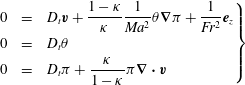 $$\begin{eqnarray}\displaystyle \left.\begin{array}{@{}rcl@{}}\displaystyle 0 & = & \displaystyle D_{t}\boldsymbol{v}+\frac{1-\unicode[STIX]{x1D705}}{\unicode[STIX]{x1D705}}\frac{1}{Ma^{2}}\unicode[STIX]{x1D703}\unicode[STIX]{x1D735}\unicode[STIX]{x1D70B}+\frac{1}{Fr^{2}}\boldsymbol{e}_{z}\\ \displaystyle 0 & = & \displaystyle D_{t}\unicode[STIX]{x1D703}\\ \displaystyle 0 & = & \displaystyle D_{t}\unicode[STIX]{x1D70B}+\frac{\unicode[STIX]{x1D705}}{1-\unicode[STIX]{x1D705}}\unicode[STIX]{x1D70B}\unicode[STIX]{x1D735}\boldsymbol{\cdot }\boldsymbol{v}\end{array}\right\} & & \displaystyle\end{eqnarray}$$
with
 $(x,z)$
the horizontal and vertical coordinates and
 $\boldsymbol{e}_{x}$
and
 $\boldsymbol{e}_{z}$
the corresponding unit vectors. Here,
 $D_{t}=\unicode[STIX]{x2202}_{t}+\boldsymbol{v}\boldsymbol{\cdot }\unicode[STIX]{x1D735}$
is the material derivative. The velocity vector field is denoted by
 $\boldsymbol{v}$
. The Exner pressure is related to the usual pressure by
 $$\begin{eqnarray}\unicode[STIX]{x1D70B}=p^{\unicode[STIX]{x1D705}},\end{eqnarray}$$
where
 $\unicode[STIX]{x1D705}=2/7$
is the ratio of the ideal gas constant
 $R$
to the specific heat capacity at constant pressure
 $c_{p}$
. From the temperature
 $T$
we define the potential temperature to be
 $$\begin{eqnarray}\unicode[STIX]{x1D703}=T/\unicode[STIX]{x1D70B}.\end{eqnarray}$$
The independent and dependent variables are non-dimensionalized according to table 1. The Mach and the Froude numbers are given by
 $Ma=v_{ref}/C_{s}$
and
 $Fr=v_{ref}/\sqrt{gL_{ref}}$
where
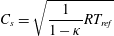 $$\begin{eqnarray}C_{s}=\sqrt{\frac{1}{1-\unicode[STIX]{x1D705}}RT_{ref}}\end{eqnarray}$$
is the speed of sound and
 $g$
the gravitational acceleration. Let
 $H_{p},H_{\unicode[STIX]{x1D703}}$
,
 $L_{ref}$
and
 $N_{ref}$
denote the pressure and potential temperature scale height, a typical wavelength and the reference Brunt–Väisälä frequency, respectively. The distinguished asymptotic limit adopted by Grimshaw (Reference Grimshaw1974) and Achatz et al. (Reference Achatz, Klein and Senf2010) is reproduced by assuming:
-
(i) low Mach number,
(2.5) $$\begin{eqnarray}\sqrt{\frac{\unicode[STIX]{x1D705}}{1-\unicode[STIX]{x1D705}}}Ma=\unicode[STIX]{x1D700}\ll 1;\end{eqnarray}$$
-
(ii) leading-order stable stratification,
(2.6)
$$\begin{eqnarray}\frac{H_{p}}{\overline{\unicode[STIX]{x1D6E9}}}\frac{\text{d}\overline{\unicode[STIX]{x1D6E9}}}{\text{d}z}=O(1)\;(\unicode[STIX]{x1D700}\rightarrow 0)\quad \text{where }H_{p}=\frac{RT_{ref}}{g}\approx 10~\text{km};\end{eqnarray}$$
-
(iii) non-hydrostatic motions,
(2.7)
$$\begin{eqnarray}x_{ref}=z_{ref}\equiv L_{ref}\approx 4~\text{km};\quad \text{and}\end{eqnarray}$$
-
(iv) large internal wave Froude number
(2.8)
$$\begin{eqnarray}Fr_{int}=\frac{v_{ref}}{N_{ref}L_{ref}}=O(1)\;(\text{as }\unicode[STIX]{x1D700}\rightarrow 0)\quad \text{where }N_{ref}=\sqrt{\frac{g}{\overline{\unicode[STIX]{x1D6E9}}}\frac{\text{d}\overline{\unicode[STIX]{x1D6E9}}}{\text{d}z}}\approx 0.02~\text{Hz}.\end{eqnarray}$$
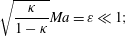



On account of (2.5), (2.6) and (2.8) we find that
 $L_{ref}/H_{p}=O(\unicode[STIX]{x1D700})$
, and we let
 $$\begin{eqnarray}L_{ref}=\unicode[STIX]{x1D700}H_{\unicode[STIX]{x1D703}}\quad \text{where }H_{\unicode[STIX]{x1D703}}=H_{p}/\unicode[STIX]{x1D705}\approx 40~\text{km}\end{eqnarray}$$
for specificity. Combining the scaling assumptions (i)–(iv), we obtain the distinguished limit
 $Fr=\unicode[STIX]{x1D700}^{1/2}$
which links the Froude number to the Mach number, so that
 $\unicode[STIX]{x1D700}$
is the only parameter appearing in (2.1).
Non-dimensionalization of variables.

2.2 Asymptotic scalings
Here we prepare the ground for the subsequent summary of the WKB analysis in § 3 by anticipating the essential spatio-temporal and amplitude scalings of the dependent variables from Achatz et al. (Reference Achatz, Klein and Senf2010). Let
 $$\begin{eqnarray}(X,Z,T)=(\unicode[STIX]{x1D700}x,\unicode[STIX]{x1D700}z,\unicode[STIX]{x1D700}t)\end{eqnarray}$$
denote compressed coordinates that resolve spatial scales comparable to the pressure scale height and the associated advection time scale. Furthermore, for any variable
 $V$
, let
 $$\begin{eqnarray}V_{0}(Z)\quad \text{and}\quad V_{\unicode[STIX]{x1D700}}^{(i)}(x,z,t;\unicode[STIX]{x1D700})\end{eqnarray}$$
denote its slowly varying leading-order horizontal background and the collection of its
 $i$
th and higher-order contributions in
 $\unicode[STIX]{x1D700}$
with wave-induced variations on the fast and slow scales. Then the asymptotic scaling of the WKB solutions to be discussed below can be summarized as
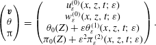 $$\begin{eqnarray}\displaystyle \left(\begin{array}{@{}c@{}}\boldsymbol{v}\\ \unicode[STIX]{x1D703}\\ \unicode[STIX]{x03C0}\end{array}\right)=\left(\begin{array}{@{}c@{}}u_{\unicode[STIX]{x1D700}}^{(0)}(x,z,t;\unicode[STIX]{x1D700})\\ w_{\unicode[STIX]{x1D700}}^{(0)}(x,z,t;\unicode[STIX]{x1D700})\\ \unicode[STIX]{x1D703}_{0}(Z)+\unicode[STIX]{x1D700}\unicode[STIX]{x1D703}_{\unicode[STIX]{x1D700}}^{(1)}(x,z,t;\unicode[STIX]{x1D700})\\ \unicode[STIX]{x1D70B}_{0}(Z)+\unicode[STIX]{x1D700}^{2}\unicode[STIX]{x1D70B}_{\unicode[STIX]{x1D700}}^{(2)}(x,z,t;\unicode[STIX]{x1D700})\end{array}\right). & & \displaystyle\end{eqnarray}$$
In the velocity field the wave appears at
 $O(1)$
, whereas potential temperature and Exner pressure decompose into leading-order hydrostatic background variations
 $\unicode[STIX]{x1D703}_{0}$
and
 $\unicode[STIX]{x1D70B}_{0}$
satisfying
 $$\begin{eqnarray}\frac{\text{d}\unicode[STIX]{x1D70B}_{0}}{\text{d}Z}=-\frac{1}{\unicode[STIX]{x1D703}_{0}},\end{eqnarray}$$
and higher-order fluctuations. Potential temperature perturbations are of order
 $O(\unicode[STIX]{x1D700})$
, whereas Exner pressure deviations appear first at
 $O(\unicode[STIX]{x1D700}^{2})$
. See Achatz et al. (Reference Achatz, Klein and Senf2010) and § 3 below for more detail.
For later reference, we use the ideal gas equation of state to express the leading-order density and temperature as
 $$\begin{eqnarray}\unicode[STIX]{x1D70C}_{0}=\frac{\unicode[STIX]{x1D70B}_{0}^{(1-\unicode[STIX]{x1D705})/\unicode[STIX]{x1D705}}}{\unicode[STIX]{x1D703}_{0}}\end{eqnarray}$$
and
 $$\begin{eqnarray}T_{0}=\unicode[STIX]{x1D703}_{0}\unicode[STIX]{x1D70B}_{0},\end{eqnarray}$$
respectively. In addition we also define the ‘logarithmic background derivative’ of any
 $f_{0}\in \{\unicode[STIX]{x1D703}_{0},\unicode[STIX]{x1D70B}_{0},\unicode[STIX]{x1D70C}_{0},T_{0}\}$
by
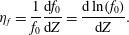 $$\begin{eqnarray}\unicode[STIX]{x1D702}_{f}=\frac{1}{f_{0}}\frac{\text{d}f_{0}}{\text{d}Z}=\frac{\text{d}\ln (f_{0})}{\text{d}Z}.\end{eqnarray}$$
Taking the derivative with respect to
 $Z$
of (2.14) and substituting with (2.16) we find that
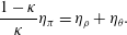 $$\begin{eqnarray}\frac{1-\unicode[STIX]{x1D705}}{\unicode[STIX]{x1D705}}\unicode[STIX]{x1D702}_{\unicode[STIX]{x1D70B}}=\unicode[STIX]{x1D702}_{\unicode[STIX]{x1D70C}}+\unicode[STIX]{x1D702}_{\unicode[STIX]{x1D703}}.\end{eqnarray}$$
We can identify
 $\unicode[STIX]{x1D702}_{\unicode[STIX]{x1D703}}=N^{2}$
as the local Brunt–Väisälä frequency squared, and
 $-\unicode[STIX]{x1D702}_{\unicode[STIX]{x1D70C}}^{-1}$
may be interpreted as the local density scale height. Combining (2.13)–(2.17), it turns out that all background variables can be expressed by the background temperature,
 $$\begin{eqnarray}\unicode[STIX]{x1D702}_{\unicode[STIX]{x1D70C}}=-\unicode[STIX]{x1D702}_{T}-\frac{1}{\unicode[STIX]{x1D705}T_{0}}\quad \text{and}\quad N^{2}=\unicode[STIX]{x1D702}_{T}+\frac{1}{T_{0}}.\end{eqnarray}$$
So once the vertical background temperature profile is known, all profiles of the remaining background variables are determined. If we now insert the distinguished limit (2.9) as well as the multiple-scale representation from (2.12) into the Euler equations (2.1) and substitute by (2.17), we arrive at a system of evolution equations
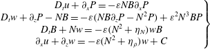 $$\begin{eqnarray}\left.\begin{array}{@{}c@{}}\displaystyle D_{t}u+\unicode[STIX]{x2202}_{x}P=-\unicode[STIX]{x1D700}NB\unicode[STIX]{x2202}_{x}P\\ \displaystyle D_{t}w+\unicode[STIX]{x2202}_{z}P-NB=-\unicode[STIX]{x1D700}(NB\unicode[STIX]{x2202}_{z}P-N^{2}P)+\unicode[STIX]{x1D700}^{2}N^{3}BP\\ \displaystyle D_{t}B+Nw=-\unicode[STIX]{x1D700}(N^{2}+\unicode[STIX]{x1D702}_{N})wB\\ \displaystyle \unicode[STIX]{x2202}_{x}u+\unicode[STIX]{x2202}_{z}w=\displaystyle -\unicode[STIX]{x1D700}(N^{2}+\unicode[STIX]{x1D702}_{\unicode[STIX]{x1D70C}})w+C\end{array}\right\}\end{eqnarray}$$
for the new set of prognostic variables
 $$\begin{eqnarray}\boldsymbol{U}=(u,w,B,P)^{\text{T}}:=\left(u_{\unicode[STIX]{x1D700}}^{(0)},w_{\unicode[STIX]{x1D700}}^{(0)},\frac{1}{N}\frac{\unicode[STIX]{x1D703}_{\unicode[STIX]{x1D700}}^{(1)}}{\unicode[STIX]{x1D703}_{0}},\unicode[STIX]{x1D703}_{0}\unicode[STIX]{x1D70B}_{\unicode[STIX]{x1D700}}^{(2)}\right)^{\text{T}},\end{eqnarray}$$
where
 $B$
and
 $P$
relate to the buoyancy and the kinetic pressure, respectively.
The expression
 $$\begin{eqnarray}C=\unicode[STIX]{x1D700}^{2}(N^{2}+\unicode[STIX]{x1D702}_{\unicode[STIX]{x1D70C}})\left(D_{t}P+\frac{\unicode[STIX]{x1D705}}{1-\unicode[STIX]{x1D705}}P(\unicode[STIX]{x2202}_{x}u+\unicode[STIX]{x2202}_{z}w)\right)-\unicode[STIX]{x1D700}^{3}(N^{2}+\unicode[STIX]{x1D702}_{\unicode[STIX]{x1D70C}})N^{2}wP\end{eqnarray}$$
in (2.19) represents higher-order terms which do not contribute to the leading-order WKB solutions because either they are literally of higher order and just do not appear, or they do appear in the expanded equations up to the order considered but cancel each other. We note in passing that (2.19) without the
 $C$
-terms constitutes Durran’s pseudo-incompressible model equations, and this corroborates the conclusion of Achatz et al. (Reference Achatz, Klein and Senf2010) that the full compressible and pseudo-incompressible models share the WKB wave packet solutions in the considered flow regime. We will refer to system (2.19) henceforth as the scaled Euler equations.
3 WKB theory for finite-amplitude gravity waves with non-uniform stratification
In this section we will apply a weak asymptotic scheme to derive the modulation equations whose travelling wave solutions are the main objective of this survey.
3.1 A spectral WKB expansion
The scaled Euler equations are a set of nonlinear, first-order partial differential equations (PDEs) whose coefficients depend only on the stretched coordinate
 $Z$
due to the background stratification. To account for the nonlinearities we exploit an asymptotic spectral expansion approach,
 $$\begin{eqnarray}\boldsymbol{U}=\mathop{\sum }_{n=0}^{M}\mathop{\sum }_{|m|\leqslant n+1}\unicode[STIX]{x1D700}^{n}\hat{U} _{n,m}\text{e}^{\text{i}m\unicode[STIX]{x1D700}^{-1}\unicode[STIX]{x1D6F7}}+o(\unicode[STIX]{x1D700}^{M}),\end{eqnarray}$$
for the vector (2.20). The subscript
 $n$
keeps track of the order in
 $\unicode[STIX]{x1D700}$
while the
 $m$
-subscript carries the order of the harmonics. So, resonant coupling of the wave with the mean flow, i.e. zeroth harmonics, occurs already at leading order (Chu & Mei Reference Chu and Mei1970; Miura & Kruskal Reference Miura and Kruskal1974). We restrict
 $\hat{U} _{n,-m}=\hat{U} _{n,m}^{\ast }$
to maintain real values, where
 $^{\ast }$
indicates the complex conjugate of a variable. To account for the slowly varying background state we apply the WKB assumption that the coefficients and the phase are functions of only the slow variables
 $(X,Z,T)$
, such that
 $$\begin{eqnarray}(X,Z,T)\mapsto \hat{U} _{n,m}(X,Z,T),\;\unicode[STIX]{x1D6F7}(X,Z,T).\end{eqnarray}$$
The differential operators become
 $$\begin{eqnarray}\unicode[STIX]{x2202}_{t}=\unicode[STIX]{x1D700}\unicode[STIX]{x2202}_{T}\quad \text{and}\quad \unicode[STIX]{x1D735}=\unicode[STIX]{x1D700}\unicode[STIX]{x1D735}_{\unicode[STIX]{x1D700}}=\unicode[STIX]{x1D700}(\unicode[STIX]{x2202}_{X},\unicode[STIX]{x2202}_{Z})^{\text{T}}.\end{eqnarray}$$
The phase should be also expanded in
 $\unicode[STIX]{x1D700}$
, like
 $$\begin{eqnarray}\unicode[STIX]{x1D6F7}=\unicode[STIX]{x1D6F7}^{(0)}+\unicode[STIX]{x1D700}^{2}\unicode[STIX]{x1D6F7}^{(2)}+O(\unicode[STIX]{x1D700}^{4}).\end{eqnarray}$$
We need only the even gauge functions because effects of any
 $\unicode[STIX]{x1D6F7}^{(1)}$
are already captured by
 $\arg (\hat{U} _{0,1})$
. Similarly, higher-order odd phases are also included in the corresponding coefficients. Since we will only analyse the system up to
 $M=1$
, these higher-order effects do not matter in this work, so we keep simply
 $\unicode[STIX]{x1D6F7}\equiv \unicode[STIX]{x1D6F7}^{(0)}$
. By means of (3.3) we can define the local wave vector and the frequency,
 $$\begin{eqnarray}\displaystyle & \displaystyle \unicode[STIX]{x1D714}=-\unicode[STIX]{x2202}_{T}\unicode[STIX]{x1D6F7}, & \displaystyle\end{eqnarray}$$
 $$\begin{eqnarray}\displaystyle & \displaystyle \boldsymbol{k}=\unicode[STIX]{x1D735}_{\unicode[STIX]{x1D700}}\unicode[STIX]{x1D6F7}. & \displaystyle\end{eqnarray}$$
By inserting the ansatz (3.1) into the governing equations (2.19), we obtain an equation of the form
 $$\begin{eqnarray}\mathop{\sum }_{k=0}^{M}\mathop{\sum }_{|l|\leqslant k+2}\unicode[STIX]{x1D700}^{k}{\mathcal{C}}_{k,l}(X,Z,T)\text{e}^{\text{i}l\unicode[STIX]{x1D700}^{-1}\unicode[STIX]{x1D6F7}(X,Z,T)}+o(\unicode[STIX]{x1D700}^{M})=0.\end{eqnarray}$$
The coefficients
 ${\mathcal{C}}_{k,l}$
represent the terms which contain the ansatz functions
 $\hat{U} _{n,m},\unicode[STIX]{x1D6F7}$
, their derivatives and the background variables. One can now establish that in the limit
 $\unicode[STIX]{x1D700}\rightarrow 0$
the coefficients must vanish independently of the order in
 $\unicode[STIX]{x1D700}$
and the order of the harmonics, i.e.
 ${\mathcal{C}}_{k,l}=0$
for all possible
 $k$
and
 $l$
. The result is an equation hierarchy providing constraints on the ansatz functions which will give us the modulation equations. In order to achieve independence with respect to the harmonics Whitham (Reference Whitham1965), Grimshaw (Reference Grimshaw1974), Miura & Kruskal (Reference Miura and Kruskal1974) and Tabaei & Akylas (Reference Tabaei and Akylas2007) assumed a priori that the solution vector
 $\boldsymbol{U}$
is, in addition to its spatio-temporal dependence, also a periodic function of the fast phase
 $\unicode[STIX]{x1D700}^{-1}\unicode[STIX]{x1D6F7}$
, so
 $$\begin{eqnarray}\boldsymbol{U}(\unicode[STIX]{x1D700}^{-1}\unicode[STIX]{x1D6F7},X,Z,T;\unicode[STIX]{x1D700})=\boldsymbol{U}(\unicode[STIX]{x1D700}^{-1}\unicode[STIX]{x1D6F7}+2\unicode[STIX]{x03C0},X,Z,T;\unicode[STIX]{x1D700}).\end{eqnarray}$$
If one now averages (3.7) with respect to the fast phase over a period
 $2\unicode[STIX]{x03C0}$
, then one can exploit the fact that the harmonics are mutually orthogonal. In terms of this argument it was justified that the claim of independently vanishing coefficients must hold with regard to the average.
We encounter two issues when we want to apply this technique to our approach in order to establish independently vanishing coefficients: (i) the fast phase depends on
 $\unicode[STIX]{x1D700}$
and (ii) it also depends itself on space and time. Due to these properties the assumption of periodicity must be justified in terms of the asymptotic series expansion of
 $\boldsymbol{U}$
. Miura & Kruskal (Reference Miura and Kruskal1974), who applied the nonlinear WKB method to the Korteweg–DeVries equation, wrote in this regard: ‘it remains unsettled whether or in what sense the series
 $\boldsymbol{U}\,[\ldots ]$
approximates the solution of the original problem’. However, we show in appendix A an alternative approach where periodicity is not needed by introducing the notion of weak asymptotic solutions based on Danilov, Omelyanov & Shelkovich (Reference Danilov, Omelyanov, Shelkovich and Karasev2003). It requires only that the ansatz functions be twice differentiable and is hence more general than the averaging method. The key ideas for overcoming the aforementioned issues are (i) to formulate (3.7) in a weak sense and (ii) to replace the Cartesian coordinates by a map onto some phase-following coordinates.
3.2 Leading-order analysis
In the following sections we present the equation hierarchy obtained by the weak asymptotic analysis. From
 ${\mathcal{C}}_{0,0}=0$
we find solenoidality of the velocity field of the primary harmonics,
 $$\begin{eqnarray}\text{i}k_{x}\hat{u} _{0,1}+\text{i}k_{z}{\hat{w}}_{0,1}=0,\end{eqnarray}$$
and constraints for some mean-flow components (the zeroth harmonics),
 $$\begin{eqnarray}\hat{B}_{0,0}={\hat{w}}_{0,0}=0.\end{eqnarray}$$
From
 ${\mathcal{C}}_{0,1}=0$
we get a linear homogeneous system of equations for the primary harmonics,
 $$\begin{eqnarray}\unicode[STIX]{x1D648}(-\text{i}\hat{\unicode[STIX]{x1D714}},\text{i}\boldsymbol{k})\hat{U} _{0,1}=0,\end{eqnarray}$$
with the anti-Hermitian coefficient matrix
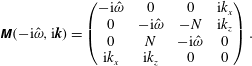 $$\begin{eqnarray}\unicode[STIX]{x1D648}(-\text{i}\hat{\unicode[STIX]{x1D714}},\text{i}\boldsymbol{k})=\left(\begin{array}{@{}cccc@{}}-\text{i}\hat{\unicode[STIX]{x1D714}} & 0 & 0 & \text{i}k_{x}\\ 0 & -\text{i}\hat{\unicode[STIX]{x1D714}} & -N & \text{i}k_{z}\\ 0 & N & -\text{i}\hat{\unicode[STIX]{x1D714}} & 0\\ \text{i}k_{x} & \text{i}k_{z} & 0 & 0\end{array}\right).\end{eqnarray}$$
Here,
 $\hat{\unicode[STIX]{x1D714}}=\unicode[STIX]{x1D714}-\hat{u} _{0,0}k_{x}$
represents the intrinsic frequency, which is the frequency one observes in a reference frame moving with the leading-order mean flow. It differs from
 $\unicode[STIX]{x1D714}$
only by a Doppler shift term. Equations
 ${\mathcal{C}}_{0,2}=0$
hold by the same solenoidality (3.9).
3.3 First-order analysis
From
 ${\mathcal{C}}_{1,0}=0$
we obtain next-order constraints for the mean flow:
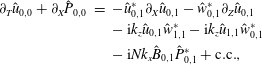 $$\begin{eqnarray}\displaystyle \unicode[STIX]{x2202}_{T}\hat{u} _{0,0}+\unicode[STIX]{x2202}_{X}\hat{P}_{0,0} & = & \displaystyle -\hat{u} _{0,1}^{\ast }\unicode[STIX]{x2202}_{X}\hat{u} _{0,1}-{\hat{w}}_{0,1}^{\ast }\unicode[STIX]{x2202}_{Z}\hat{u} _{0,1}\nonumber\\ \displaystyle & & \displaystyle -\,\text{i}k_{z}\hat{u} _{0,1}{\hat{w}}_{1,1}^{\ast }-\text{i}k_{z}\hat{u} _{1,1}{\hat{w}}_{0,1}^{\ast }\nonumber\\ \displaystyle & & \displaystyle -\,\text{i}Nk_{x}\hat{B}_{0,1}\hat{P}_{0,1}^{\ast }+\text{c.c.},\end{eqnarray}$$
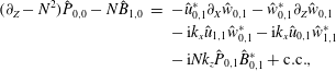 $$\begin{eqnarray}\displaystyle (\unicode[STIX]{x2202}_{Z}-N^{2})\hat{P}_{0,0}-N\hat{B}_{1,0} & = & \displaystyle -\hat{u} _{0,1}^{\ast }\unicode[STIX]{x2202}_{X}{\hat{w}}_{0,1}-{\hat{w}}_{0,1}^{\ast }\unicode[STIX]{x2202}_{Z}{\hat{w}}_{0,1}\nonumber\\ \displaystyle & & \displaystyle -\,\text{i}k_{x}\hat{u} _{1,1}{\hat{w}}_{0,1}^{\ast }-\text{i}k_{x}\hat{u} _{0,1}{\hat{w}}_{1,1}^{\ast }\nonumber\\ \displaystyle & & \displaystyle -\,\text{i}Nk_{z}\hat{P}_{0,1}\hat{B}_{0,1}^{\ast }+\text{c.c.},\end{eqnarray}$$
 $$\begin{eqnarray}\displaystyle N{\hat{w}}_{1,0} & = & \displaystyle -\hat{u} _{0,1}^{\ast }\unicode[STIX]{x2202}_{X}\hat{B}_{0,1}-{\hat{w}}_{0,1}^{\ast }\unicode[STIX]{x2202}_{Z}\hat{B}_{0,1}\nonumber\\ \displaystyle & & \displaystyle -\,(N^{2}+\unicode[STIX]{x1D702}_{N}){\hat{w}}_{0,1}^{\ast }\hat{B}_{0,1}+\text{c.c.},\end{eqnarray}$$
 $$\begin{eqnarray}\displaystyle \unicode[STIX]{x2202}_{X}\hat{u} _{0,0} & = & \displaystyle 0,\end{eqnarray}$$
where
 $\text{c.c.}$
stands for the complex conjugate of the previous terms. Primary harmonics are fixed by
 ${\mathcal{C}}_{1,1}=0$
: it follows a linear inhomogeneous system for
 $\hat{U} _{1,1}$
,
 $$\begin{eqnarray}\unicode[STIX]{x1D648}(-\text{i}\hat{\unicode[STIX]{x1D714}},\text{i}\boldsymbol{k})\hat{U} _{1,1}=-\unicode[STIX]{x1D64D}(\hat{U} _{1,2},\text{i}\boldsymbol{k})\hat{U} _{0,-1}-\boldsymbol{L}(\unicode[STIX]{x1D6FF}_{T},\unicode[STIX]{x1D735}_{\unicode[STIX]{x1D700}})\hat{U} _{0,1},\end{eqnarray}$$
with
 $\unicode[STIX]{x1D64D}$
being a matrix
 $$\begin{eqnarray}\unicode[STIX]{x1D64D}(\hat{U} _{1,2},\text{i}\boldsymbol{k})=\left(\begin{array}{@{}cccc@{}}\text{i}k_{x}\hat{u} _{1,2}-\text{i}k_{z}{\hat{w}}_{1,2} & 2\text{i}k_{z}\hat{u} _{1,2} & 0 & 0\\ 2\text{i}k_{x}{\hat{w}}_{1,2} & \text{i}k_{z}{\hat{w}}_{1,2}-\text{i}k_{x}\hat{u} _{1,2} & 0 & 0\\ 2\text{i}k_{x}\hat{B}_{1,2} & 2\text{i}k_{z}\hat{B}_{1,2} & -\text{i}k_{x}\hat{u} _{1,2}-\text{i}k_{z}{\hat{w}}_{1,2} & 0\\ 0 & 0 & 0 & 0\end{array}\right)\end{eqnarray}$$
and
 $\boldsymbol{L}$
being a linear differential operator
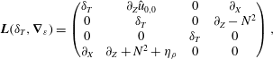 $$\begin{eqnarray}\boldsymbol{L}(\unicode[STIX]{x1D6FF}_{T},\unicode[STIX]{x1D735}_{\unicode[STIX]{x1D700}})=\left(\begin{array}{@{}cccc@{}}\unicode[STIX]{x1D6FF}_{T} & \unicode[STIX]{x2202}_{Z}\hat{u} _{0,0} & 0 & \unicode[STIX]{x2202}_{X}\\ 0 & \unicode[STIX]{x1D6FF}_{T} & 0 & \unicode[STIX]{x2202}_{Z}-N^{2}\\ 0 & 0 & \unicode[STIX]{x1D6FF}_{T} & 0\\ \unicode[STIX]{x2202}_{X} & \unicode[STIX]{x2202}_{Z}+N^{2}+\unicode[STIX]{x1D702}_{\unicode[STIX]{x1D70C}} & 0 & 0\end{array}\right),\end{eqnarray}$$
where
 $\unicode[STIX]{x1D6FF}_{T}=\unicode[STIX]{x2202}_{T}+\hat{u} _{0,0}\unicode[STIX]{x2202}_{X}+\text{i}k_{x}\hat{u} _{1,0}+\text{i}k_{z}{\hat{w}}_{1,0}$
. Equations
 ${\mathcal{C}}_{1,2}={\mathcal{C}}_{1,3}=0$
yield the solenoidality,
 $$\begin{eqnarray}\text{i}k_{x}\hat{u} _{1,2}+\text{i}k_{z}{\hat{w}}_{1,2}=0,\end{eqnarray}$$
for the velocity field of the secondary harmonics.
3.4 Second-order analysis
From
 ${\mathcal{C}}_{2,0}=0$
we obtain, among others,
 $$\begin{eqnarray}\unicode[STIX]{x2202}_{X}\hat{u} _{1,0}+(\unicode[STIX]{x2202}_{Z}+N^{2}+\unicode[STIX]{x1D702}_{\unicode[STIX]{x1D70C}}){\hat{w}}_{1,0}=0.\end{eqnarray}$$
Here, we have already used the solenoidality (3.9). At this point we can stop the iteration as we have found enough constraints to construct leading-order solutions.
3.5 Derivation of the modulation equations
The objective of this section is to exploit solvability constraints from the asymptotic analysis (3.9)–(3.21) in order to derive a closed set of equations which we will refer to as modulation equations. Equation (3.11) has non-trivial solution only if
 $\det (\unicode[STIX]{x1D648})=0$
, yielding the dispersion relation
 $$\begin{eqnarray}\hat{\unicode[STIX]{x1D714}}^{2}=\frac{N^{2}k_{x}^{2}}{k_{x}^{2}+k_{z}^{2}}.\end{eqnarray}$$
Note that
 $\text{sgn}(\hat{\unicode[STIX]{x1D714}})=\pm 1$
indicates two different branches of the solution. By definition (3.5), the dispersion relation is essentially a prognostic equation for
 $\unicode[STIX]{x1D6F7}$
, which is by definition (3.6) in the form of a Hamilton–Jacobi equation. We find a particular vector
 ${\mathcal{U}}\in \ker (\unicode[STIX]{x1D648})$
providing the polarization relation
 $$\begin{eqnarray}{\mathcal{U}}(\hat{\unicode[STIX]{x1D714}},\boldsymbol{k})=\left(-\text{i}\frac{k_{z}}{k_{x}}\frac{\hat{\unicode[STIX]{x1D714}}}{N},\text{i}\frac{\hat{\unicode[STIX]{x1D714}}}{N},1,-\text{i}\frac{k_{z}}{k_{x}^{2}}\frac{\hat{\unicode[STIX]{x1D714}}^{2}}{N}\right)^{\text{T}},\end{eqnarray}$$
which is exactly the same polarization one would obtain in Boussinesq theory. For a detailed discussion on polarization relations in different soundproof approximations we refer to Davies et al. (Reference Davies, Staniforth, Wood and Thuburn2003). We deduce that
 $\operatorname{rank}(\unicode[STIX]{x1D648})=3$
. Since
 $\dim (\ker (\unicode[STIX]{x1D648}))=1$
, we get a general solution for (3.11) by
 $$\begin{eqnarray}\hat{U} _{0,1}=A{\mathcal{U}}(\hat{\unicode[STIX]{x1D714}},\boldsymbol{k})\quad \text{where }\hat{U} _{0,1}=(\hat{u} _{0,1},{\hat{w}}_{0,1},\hat{B}_{0,1},\hat{P}_{0,1})^{\text{T}},\end{eqnarray}$$
with a complex-valued scalar
 $A$
that we later refer to as the wave amplitude. Note in particular that
 $\hat{B}_{0,1}\equiv A$
. By means of solenoidality of the several harmonics in the velocity, (3.9) and (3.20), we can show that
 $\unicode[STIX]{x1D64D}(\hat{U} _{1,2},\boldsymbol{k})\hat{U} _{0,-1}=0$
, which simplifies (3.17). A necessary condition for the solvability of (3.17) is that any vector
 $\boldsymbol{L}\hat{U} _{0,1}\in \operatorname{img}(\unicode[STIX]{x1D648})$
has to be orthogonal to every
 ${\mathcal{U}}\in \ker (\unicode[STIX]{x1D648})$
by the rank–nullity theorem:
 $$\begin{eqnarray}0={\mathcal{U}}^{\ast T}\boldsymbol{L}\hat{U} _{0,1}.\end{eqnarray}$$
If equation (3.25) holds, then
 $$\begin{eqnarray}\displaystyle & \displaystyle 0=\hat{U} _{0,1}^{\ast T}\boldsymbol{L}\hat{U} _{0,1}+\text{c.c.}, & \displaystyle\end{eqnarray}$$
 $$\begin{eqnarray}\displaystyle & \displaystyle 0=\hat{U} _{0,1}^{\ast T}\boldsymbol{L}\hat{U} _{0,1}-\text{c.c.} & \displaystyle\end{eqnarray}$$
must be true independently, if
 $A\neq 0$
, which will serve to fix the degrees of freedom in
 $$\begin{eqnarray}A=|A|\exp (\text{i}\arg (A)).\end{eqnarray}$$
This argument essentially means that the real and imaginary parts of the right-hand side of (3.25) must vanish. Equation (3.26) is true if
 $$\begin{eqnarray}\unicode[STIX]{x2202}_{T}|A|^{2}+(\unicode[STIX]{x1D735}_{\unicode[STIX]{x1D700}}+\unicode[STIX]{x1D702}_{\unicode[STIX]{x1D70C}}\boldsymbol{e}_{z})\boldsymbol{\cdot }(\boldsymbol{c}_{g}|A|^{2})+|A|^{2}\frac{k_{x}}{\hat{\unicode[STIX]{x1D714}}}\frac{\unicode[STIX]{x2202}\hat{\unicode[STIX]{x1D714}}}{\unicode[STIX]{x2202}k_{z}}\unicode[STIX]{x2202}_{Z}\hat{u} _{0,0}=0,\end{eqnarray}$$
which is derived using (3.16). This equation of motion yields essentially the evolution of the wave energy
 $\widetilde{E}\equiv 2\unicode[STIX]{x1D70C}_{0}|A|^{2}$
, which will be extensively discussed in § 4. With the help of the consistency relations,
 $\unicode[STIX]{x2202}_{T}\boldsymbol{k}+\unicode[STIX]{x1D735}_{\unicode[STIX]{x1D700}}\unicode[STIX]{x1D714}=0$
and
 $\unicode[STIX]{x2202}_{X}k_{z}=\unicode[STIX]{x2202}_{Z}k_{x}$
, that we obtain by cross-differentiating the definitions (3.5) and (3.6), we find
 $$\begin{eqnarray}(\unicode[STIX]{x2202}_{T}+\boldsymbol{c}_{g}\boldsymbol{\cdot }\unicode[STIX]{x1D735}_{\unicode[STIX]{x1D700}})\hat{\unicode[STIX]{x1D714}}=-k_{x}\frac{\unicode[STIX]{x2202}\hat{\unicode[STIX]{x1D714}}}{\unicode[STIX]{x2202}k_{z}}\unicode[STIX]{x2202}_{Z}\hat{u} _{0,0},\end{eqnarray}$$
with the group velocity
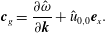 $$\begin{eqnarray}\boldsymbol{c}_{g}=\frac{\unicode[STIX]{x2202}\hat{\unicode[STIX]{x1D714}}}{\unicode[STIX]{x2202}\boldsymbol{k}}+\hat{u} _{0,0}\boldsymbol{e}_{x}.\end{eqnarray}$$
Combining
 $\unicode[STIX]{x1D70C}_{0}\times$
(3.29) with (3.30) and exploiting that
 $\unicode[STIX]{x1D70C}_{0}(\unicode[STIX]{x2202}_{Z}+\unicode[STIX]{x1D702}_{\unicode[STIX]{x1D70C}})\,\cdot \,=\unicode[STIX]{x2202}_{Z}(\unicode[STIX]{x1D70C}_{0}\,\cdot \,)$
results in a conservation law
 $$\begin{eqnarray}\unicode[STIX]{x2202}_{T}{\mathcal{A}}+\unicode[STIX]{x1D735}_{\unicode[STIX]{x1D700}}\boldsymbol{\cdot }(\boldsymbol{c}_{g}{\mathcal{A}})=0\end{eqnarray}$$
for the wave action density
 ${\mathcal{A}}=\widetilde{E}/\hat{\unicode[STIX]{x1D714}}$
.
Let us return to the orthogonality of the kernel vector and the image vector (3.25). Exploiting (3.27) gives an equation of motion for the argument of
 $A$
being basically some slow phase in addition to the fast phase
 $\unicode[STIX]{x1D700}^{-1}\unicode[STIX]{x1D6F7}$
, i.e.
 $$\begin{eqnarray}(\unicode[STIX]{x2202}_{T}+\boldsymbol{c}_{g}\boldsymbol{\cdot }\unicode[STIX]{x1D735}_{\unicode[STIX]{x1D700}})\arg (A)=-k_{x}\hat{u} _{1,0},\end{eqnarray}$$
which contains the first-order mean-flow horizontal wind. With the aid of the derivations from above, we can handle the mean-flow equations (3.13)–(3.16) and (3.21). Using once more solenoidality from (3.9) and (3.20), it is possible to settle all the terms depending on
 $\hat{U} _{1,1}$
, so
 $$\begin{eqnarray}\displaystyle & \displaystyle \unicode[STIX]{x2202}_{T}\hat{u} _{0,0}+\unicode[STIX]{x2202}_{X}\hat{P}_{0,0}=-\unicode[STIX]{x2202}_{X}|\hat{u} _{0,1}|^{2}-(\unicode[STIX]{x2202}_{Z}+\unicode[STIX]{x1D702}_{\unicode[STIX]{x1D70C}})(\hat{u} _{0,1}^{\ast }{\hat{w}}_{0,1})+\text{c.c.}, & \displaystyle\end{eqnarray}$$
 $$\begin{eqnarray}\displaystyle & \displaystyle {\hat{w}}_{1,0}=0, & \displaystyle\end{eqnarray}$$
 $$\begin{eqnarray}\displaystyle & \displaystyle \unicode[STIX]{x2202}_{X}\hat{u} _{0,0}=0, & \displaystyle\end{eqnarray}$$
 $$\begin{eqnarray}\displaystyle & \displaystyle \unicode[STIX]{x2202}_{X}\hat{u} _{1,0}=0. & \displaystyle\end{eqnarray}$$
If we plug (3.24) into (3.34), we obtain an equation of motion for the leading-order mean-flow horizontal wind,
 $$\begin{eqnarray}\unicode[STIX]{x1D70C}_{0}(\unicode[STIX]{x2202}_{T}\hat{u} _{0,0}+\unicode[STIX]{x2202}_{X}\hat{P}_{0,0})=-\unicode[STIX]{x1D735}_{\unicode[STIX]{x1D700}}\boldsymbol{\cdot }((\boldsymbol{c}_{g}-\hat{u} _{0,0}\boldsymbol{e}_{x})k_{x}{\mathcal{A}}).\end{eqnarray}$$
The six equations (3.22), (3.32), (3.33), (3.36), (3.37) and (3.38) that we derived in this section constitute a coupled system of equations for the six unknowns
 $$\begin{eqnarray}\unicode[STIX]{x1D6F7},\quad |A|,\quad \arg (A),\quad \hat{u} _{0,0},\quad \hat{P}_{0,0}\quad \text{and}\quad \hat{u} _{1,0}.\end{eqnarray}$$
These are the aforementioned modulation equations. Once they are solved, the leading-order, weak asymptotic solution of the scaled Euler equations has been found. It is worth mentioning that further solvability constraints for the first-order mean flow will show up when we keep iterating the asymptotic scheme. The equations are in line with the calculations of Achatz et al. (Reference Achatz, Klein and Senf2010). However, in addition, we provide explicitly a prognostic equation for the slow phase
 $\arg (A)$
and a constraint for the first-order mean-flow horizontal wind since they contribute to the leading-order solution. Equation (3.14) containing
 $\hat{B}_{1,0}$
can be considered to be uncoupled as it does not affect the leading-order solution and it does not appear in one of the other modulation equations.
4 Energy balance
An important aspect of wave dynamics is the energy budget. As our theory allows for a wave–mean-flow interaction, we want to investigate the energy exchange. We can rewrite (3.29) in terms of the wave energy density, which we define as
 $\widetilde{E}=2\unicode[STIX]{x1D70C}_{0}|A|^{2}$
, so
 $$\begin{eqnarray}\unicode[STIX]{x2202}_{T}\widetilde{E}+\unicode[STIX]{x1D735}_{\unicode[STIX]{x1D700}}\boldsymbol{\cdot }(\boldsymbol{c}_{g}\widetilde{E})=-c_{gz}k_{x}{\mathcal{A}}\unicode[STIX]{x2202}_{Z}\hat{u} _{0,0}.\end{eqnarray}$$
On the left-hand side we find a conservative flux that transports energy with the group velocity, and on the right-hand side is an energy source term that is associated with the vertical shear of the mean-flow horizontal wind. Let us now consider the mean-flow equation (3.38). Multiplying it by
 $\hat{u} _{0,0}$
and using the chain rule and (3.16) gives us an evolution equation for the mean-flow kinetic energy density
 $\overline{E}=\unicode[STIX]{x1D70C}_{0}\hat{u} _{0,0}^{2}/2$
, so
 $$\begin{eqnarray}\unicode[STIX]{x2202}_{T}\overline{E}+\unicode[STIX]{x1D735}_{\unicode[STIX]{x1D700}}\boldsymbol{\cdot }(\unicode[STIX]{x1D70C}_{0}\hat{u} _{0,0}\hat{P}_{0,0}\boldsymbol{e}_{x}+\boldsymbol{c}_{g}k_{x}{\mathcal{A}}\hat{u} _{0,0})=c_{gz}k_{x}{\mathcal{A}}\unicode[STIX]{x2202}_{Z}\hat{u} _{0,0}.\end{eqnarray}$$
On the left-hand side we find also a conservative flux and on the right-hand side the same energy source term as in (4.1) but with the opposite sign, making it an energy exchange rate. Hence, if we add (4.1) and (4.2), we obtain a conservation law for the total energy density
 $E=\widetilde{E}+\overline{E}$
. We will refer to the energy exchange rate, i.e. the right-hand side of (4.2), as
 $q$
. In conclusion, the total energy is conserved by the modulation equations. The sign of the exchange rate determines the direction of energy flow. For example, an upward-propagating wave packet with downward-facing phase speed vector transfers energy to the mean flow if the vertical shear is positive and vice versa.
5 Travelling wave solutions of the modulation equations
A key aspect for derivations of stability properties are travelling wave solutions. These are stationary, i.e. time-independent, solutions in a translational coordinate system moving with relative velocity
 $\boldsymbol{C}$
. Performing a coordinate transformation of the governing equations and linearizing at the travelling wave solution results in an eigenvalue problem (due to the stationarity in the translational coordinates) for the time evolution of a small perturbation. The eigenvalues tell us whether the perturbation is bounded or grows in time, which implies instability. If we find travelling waves for the modulation equations, we automatically obtain weak asymptotic travelling wave solutions for the scaled Euler equations. Consider the translational coordinate system
 $\unicode[STIX]{x1D6E4}=(\unicode[STIX]{x1D709},\unicode[STIX]{x1D701},\unicode[STIX]{x1D70F})$
defined by the transformation
 $(X,Z,T)\mapsto \unicode[STIX]{x1D6E4}(X,Z,T)$
:
 $$\begin{eqnarray}\left(\begin{array}{@{}c@{}}\unicode[STIX]{x1D709}\\ \unicode[STIX]{x1D701}\end{array}\right)=\left(\begin{array}{@{}c@{}}X\\ Z\end{array}\right)-\boldsymbol{C}T\quad \text{and}\quad \unicode[STIX]{x1D70F}=T,\end{eqnarray}$$
with
 $\boldsymbol{C}=(C_{x},C_{z})^{\text{T}}$
being the constant relative velocity. Note that the unit vectors are preserved and the mapping is one to one. The nabla operator and the time derivative become
 $$\begin{eqnarray}\unicode[STIX]{x1D735}_{\unicode[STIX]{x1D700}}=\boldsymbol{e}_{x}\unicode[STIX]{x2202}_{\unicode[STIX]{x1D709}}+\boldsymbol{e}_{z}\unicode[STIX]{x2202}_{\unicode[STIX]{x1D701}}\end{eqnarray}$$
and
 $$\begin{eqnarray}\unicode[STIX]{x2202}_{T}=\unicode[STIX]{x2202}_{\unicode[STIX]{x1D70F}}-\boldsymbol{C}\boldsymbol{\cdot }\unicode[STIX]{x1D735}_{\unicode[STIX]{x1D700}},\end{eqnarray}$$
respectively. The modulation equations in the new coordinates may be written as
 $$\begin{eqnarray}\displaystyle & \displaystyle -(\unicode[STIX]{x2202}_{\unicode[STIX]{x1D70F}}-\boldsymbol{C}\boldsymbol{\cdot }\unicode[STIX]{x1D735}_{\unicode[STIX]{x1D700}})\unicode[STIX]{x1D6F7}=\hat{\unicode[STIX]{x1D714}}(\boldsymbol{k})+\hat{u} _{0,0}k_{x}, & \displaystyle\end{eqnarray}$$
 $$\begin{eqnarray}\displaystyle & \displaystyle (\unicode[STIX]{x2202}_{\unicode[STIX]{x1D70F}}-\boldsymbol{C}\boldsymbol{\cdot }\unicode[STIX]{x1D735}_{\unicode[STIX]{x1D700}})a+(\unicode[STIX]{x1D735}_{\unicode[STIX]{x1D700}}+\unicode[STIX]{x1D702}_{\unicode[STIX]{x1D70C}}\boldsymbol{e}_{z})\boldsymbol{\cdot }(\boldsymbol{c}_{g}a)=0, & \displaystyle\end{eqnarray}$$
 $$\begin{eqnarray}\displaystyle & \displaystyle (\unicode[STIX]{x2202}_{\unicode[STIX]{x1D70F}}+(\boldsymbol{c}_{g}-\boldsymbol{C})\boldsymbol{\cdot }\unicode[STIX]{x1D735}_{\unicode[STIX]{x1D700}})\arg (A)=-k_{x}\hat{u} _{1,0}, & \displaystyle\end{eqnarray}$$
 $$\begin{eqnarray}\displaystyle & \displaystyle (\unicode[STIX]{x2202}_{\unicode[STIX]{x1D70F}}-C_{z}\unicode[STIX]{x2202}_{\unicode[STIX]{x1D701}})\hat{u} _{0,0}+\unicode[STIX]{x2202}_{\unicode[STIX]{x1D709}}\hat{P}_{0,0}=-(\unicode[STIX]{x1D735}_{\unicode[STIX]{x1D700}}+\unicode[STIX]{x1D702}_{\unicode[STIX]{x1D70C}}\boldsymbol{e}_{z})\boldsymbol{\cdot }((\boldsymbol{c}_{g}-\hat{u} _{0,0}\boldsymbol{e}_{x})k_{x}a), & \displaystyle\end{eqnarray}$$
 $$\begin{eqnarray}\displaystyle & \displaystyle \unicode[STIX]{x2202}_{\unicode[STIX]{x1D709}}\hat{u} _{0,0}=0, & \displaystyle\end{eqnarray}$$
 $$\begin{eqnarray}\displaystyle & \displaystyle \unicode[STIX]{x2202}_{\unicode[STIX]{x1D709}}\hat{u} _{1,0}=0. & \displaystyle\end{eqnarray}$$
For the sake of the following arguments, we replaced
 ${\mathcal{A}}$
by the ‘mass-specific’ wave action density
 $a=\unicode[STIX]{x1D70C}_{0}^{-1}{\mathcal{A}}$
. These equations depend on the background variables
 $N$
and
 $\unicode[STIX]{x1D702}_{\unicode[STIX]{x1D70C}}$
which are functions of
 $Z=\unicode[STIX]{x1D701}+C_{z}\unicode[STIX]{x1D70F}$
due to the transformation, so they now depend in particular on time. In other words, the background in the translational reference frame is not hydrostatic anymore since the frame moves relatively to the background. We conclude that stationary solutions can only exist in two disjoint cases:
-
(C1) The reference frame does not move vertically, such that
$C_{z}=0$
. In this case we find that
$Z=\unicode[STIX]{x1D701}$
and hence the background is again time-independent. We will refer to this case as the horizontally travelling wave solution. It will be examined in § 5.1. -
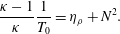
(C2) The background variables are constant in the first place and in general
$C_{z}\neq 0$
. If we combine the definition of the background temperature (2.15) with (2.17), we obtain (5.10)From this brief calculation we can deduce that the background temperature must be constant if the right-hand side is constant. Because of this point we will refer to this case as the isothermal travelling wave solution, which will be investigated in § 5.2.
$$\begin{eqnarray}\frac{\unicode[STIX]{x1D705}-1}{\unicode[STIX]{x1D705}}\frac{1}{T_{0}}=\unicode[STIX]{x1D702}_{\unicode[STIX]{x1D70C}}+N^{2}.\end{eqnarray}$$


In both cases, a stationary solution in the co-moving reference frame to (5.4) is given by
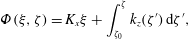 $$\begin{eqnarray}\unicode[STIX]{x1D6F7}(\unicode[STIX]{x1D709},\unicode[STIX]{x1D701})=K_{x}\unicode[STIX]{x1D709}+\int _{\unicode[STIX]{x1D701}_{0}}^{\unicode[STIX]{x1D701}}k_{z}(\unicode[STIX]{x1D701}^{\prime })\,\text{d}\unicode[STIX]{x1D701}^{\prime },\end{eqnarray}$$
where
 $K_{x}$
is a constant that is, without loss of generality, positive and
 $k_{z}$
is the root of the fourth-order polynomial derived from the dispersion relation
 $$\begin{eqnarray}(C_{z}k_{z}+(C_{x}-\hat{u} _{00})K_{x})^{2}=\frac{N^{2}K_{x}^{2}}{K_{x}^{2}+k_{z}^{2}}.\end{eqnarray}$$
The point
 $\unicode[STIX]{x1D701}_{0}$
denotes a reference point for the boundary conditions and may be chosen as
 $\unicode[STIX]{x1D701}_{0}=0$
, i.e. the bottom.
5.1 The horizontally travelling wave solution
In this section we want to investigate the horizontally travelling wave solution (C1), because it is possible to find analytic, explicit solutions in this case, even for arbitrary stratification. These solutions already possess some interesting properties such as nonlinear phase and amplitude, as well as arbitrary mean-flow horizontal wind.
If
 $C_{z}=0$
, then
 $\hat{u} _{0,0}$
disappears in (5.7), and hence (5.8) is solved by any real function
 $$\begin{eqnarray}\hat{u} _{0,0}(\unicode[STIX]{x1D701})=u_{f0}(\unicode[STIX]{x1D701}).\end{eqnarray}$$
Although we did not show the equation, an evolution equation for
 $\hat{u} _{1,0}$
emerges at higher order in the asymptotic iteration. But fortunately the same argument holds due to (5.9), so it turns out that
 $\hat{u} _{1,0}(\unicode[STIX]{x1D701})=u_{f1}(\unicode[STIX]{x1D701})$
is also an arbitrary function. Equation (5.12) reduces to a quadratic polynomial that is solved by
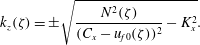 $$\begin{eqnarray}k_{z}(\unicode[STIX]{x1D701})=\pm \sqrt{\frac{N^{2}(\unicode[STIX]{x1D701})}{(C_{x}-u_{f0}(\unicode[STIX]{x1D701}))^{2}}-K_{x}^{2}}.\end{eqnarray}$$
It is worth pointing out that a negative discriminant results in exponential growth or decay of the wave in the vertical direction corresponding to a reflective layer. To prevent this, we constrain
 $N/K_{x}>|C_{z}-u_{f0}|$
at any point. Also, we must not have
 $u_{f0}=C_{x}$
at any point as it possibly causes singularities, which corresponds to a critical layer.
To solve (5.5), we drop the time derivative and rewrite it as
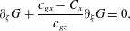 $$\begin{eqnarray}\unicode[STIX]{x2202}_{\unicode[STIX]{x1D701}}G+\frac{c_{gx}-C_{x}}{c_{gz}}\unicode[STIX]{x2202}_{\unicode[STIX]{x1D709}}G=0,\end{eqnarray}$$
which is an equation for the vertical wave action flux
 $G=\unicode[STIX]{x1D70C}_{0}c_{gz}a$
. Its validity requires that
 $c_{gz}\neq 0$
, which is fulfilled if
 $k_{z}\neq 0$
and bounded. This manipulation is feasible as
 $\boldsymbol{c}_{g}$
depends only on
 $\unicode[STIX]{x1D701}$
due to (5.13) and (5.14). As soon as we find a solution for
 $G$
, the amplitude can then be computed by
 $|A|=\sqrt{G\hat{\unicode[STIX]{x1D714}}/(2\unicode[STIX]{x1D70C}_{0}c_{gz})}$
. By the method of characteristics a solution is given by
 $$\begin{eqnarray}G(\unicode[STIX]{x1D709},\unicode[STIX]{x1D701})=G_{0}(\unicode[STIX]{x1D6F9}),\end{eqnarray}$$
with
 $$\begin{eqnarray}\unicode[STIX]{x1D6F9}(\unicode[STIX]{x1D709},\unicode[STIX]{x1D701})=K_{x}\unicode[STIX]{x1D709}-K_{x}\int _{\unicode[STIX]{x1D701}_{0}}^{\unicode[STIX]{x1D701}}\frac{c_{gx}(\unicode[STIX]{x1D701}^{\prime })-C_{x}}{c_{gz}(\unicode[STIX]{x1D701}^{\prime })}\,\text{d}\unicode[STIX]{x1D701}^{\prime }.\end{eqnarray}$$
The function
 $G_{0}$
can be determined by a boundary condition at
 $\unicode[STIX]{x1D701}_{0}$
. Equation (5.17) can be further simplified if we plug in the definition (3.31) and use the dispersion relation (5.4), yielding
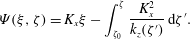 $$\begin{eqnarray}\unicode[STIX]{x1D6F9}(\unicode[STIX]{x1D709},\unicode[STIX]{x1D701})=K_{x}\unicode[STIX]{x1D709}-\int _{\unicode[STIX]{x1D701}_{0}}^{\unicode[STIX]{x1D701}}\frac{K_{x}^{2}}{k_{z}(\unicode[STIX]{x1D701}^{\prime })}\,\text{d}\unicode[STIX]{x1D701}^{\prime }.\end{eqnarray}$$
Note that the characteristic curves given through
 $\unicode[STIX]{x1D6F9}$
are locally orthogonal on every line with constant phase
 $\unicode[STIX]{x1D6F7}$
. This remarkable property will be investigated in detail in appendix B and used to construct the substitution that was postulated in order to obtain weak asymptotic solutions in § 3 and appendix A. Taking advantage of (5.9), we can compute a solution to (5.6) by separation of variables, so
 $$\begin{eqnarray}\arg (A)(\unicode[STIX]{x1D709},\unicode[STIX]{x1D701})=L_{\unicode[STIX]{x1D6F9}}\unicode[STIX]{x1D6F9}(\unicode[STIX]{x1D709},\unicode[STIX]{x1D701})-K_{x}\int _{\unicode[STIX]{x1D701}_{0}}^{\unicode[STIX]{x1D701}}\frac{u_{f1}(\unicode[STIX]{x1D701}^{\prime })}{c_{gz}(\unicode[STIX]{x1D701}^{\prime })}\,\text{d}\unicode[STIX]{x1D701}^{\prime },\end{eqnarray}$$
with
 $L_{\unicode[STIX]{x1D6F9}}$
some constant which may be interpreted as a slow wavenumber. A general solution to (5.7) is found upon inserting (5.5):
 $$\begin{eqnarray}P_{0,0}(\unicode[STIX]{x1D709},\unicode[STIX]{x1D701})=K_{x}(u_{f0}(\unicode[STIX]{x1D701})-C_{x})a(\unicode[STIX]{x1D709},\unicode[STIX]{x1D701})+P_{f}(\unicode[STIX]{x1D701}),\end{eqnarray}$$
where
 $P_{f}$
is some function.
Before we proceed to derive an explicit, analytic solution, let us consider the energy budget. With the aid of (5.16) we can compute the energy exchange rate presented in § 4 as
 $$\begin{eqnarray}q=K_{x}G\unicode[STIX]{x2202}_{Z}u_{f0}.\end{eqnarray}$$
If
 $G$
is locally confined, the energy exchange between wave and mean flow happens on the characteristic curves defined by
 $\unicode[STIX]{x1D6F9}$
, and is strongest where the characteristic curve of the peak of
 $G$
meets the level of strongest vertical shear.
We were able to derive a complete general solution in the case of a horizontally travelling wave. However, the solution is still not explicit since integrals emerged for
 $\unicode[STIX]{x1D6F7}$
,
 $\unicode[STIX]{x1D6F9}$
and
 $\arg (A)$
. They may be computed numerically, although for some particular background stratification profiles and horizontal mean-flow winds these integrals may have analytic solutions.
Consider a background with constant mean flow, such that
 $$\begin{eqnarray}u_{f0}=U_{f}=\text{const.}\quad \text{and}\quad u_{f1}=0,\end{eqnarray}$$
and a stratification profile
 $$\begin{eqnarray}N^{2}(\unicode[STIX]{x1D701})=N_{min}^{2}+(N_{max}^{2}-N_{min}^{2})\left(1+\left(\frac{\unicode[STIX]{x1D701}-\unicode[STIX]{x1D701}_{0}}{\unicode[STIX]{x0394}\unicode[STIX]{x1D701}}\right)^{2}\right)^{-2},\end{eqnarray}$$
which represents a bell function with a peak of
 $N_{max}^{2}$
centred at
 $\unicode[STIX]{x1D701}_{0}$
and width
 $\unicode[STIX]{x0394}\unicode[STIX]{x1D701}$
. For
 $\unicode[STIX]{x1D701}\rightarrow \pm \infty$
it converges to
 $N_{min}^{2}$
. When we insert these assumptions into (5.14), we obtain
 $$\begin{eqnarray}k_{z}(\unicode[STIX]{x1D701})=\pm K_{x}\frac{\sqrt{N_{max}^{2}-N_{min}^{2}}}{N_{min}}\left(1+\left(\frac{\unicode[STIX]{x1D701}-\unicode[STIX]{x1D701}_{0}}{\unicode[STIX]{x0394}\unicode[STIX]{x1D701}}\right)^{2}\right)^{-1}.\end{eqnarray}$$
Here, we chose
 $C_{x}=N_{min}/K_{x}+U_{f}$
. This can be integrated by means of standard antiderivatives, so
 $$\begin{eqnarray}\unicode[STIX]{x1D6F7}(\unicode[STIX]{x1D709},\unicode[STIX]{x1D701})=K_{x}\unicode[STIX]{x1D709}\pm K_{x}\unicode[STIX]{x0394}\unicode[STIX]{x1D701}\frac{\sqrt{N_{max}^{2}-N_{min}^{2}}}{N_{min}}\arctan \left(\frac{\unicode[STIX]{x1D701}-\unicode[STIX]{x1D701}_{0}}{\unicode[STIX]{x0394}\unicode[STIX]{x1D701}}\right)\end{eqnarray}$$
and
 $$\begin{eqnarray}\unicode[STIX]{x1D6F9}(\unicode[STIX]{x1D709},\unicode[STIX]{x1D701})=K_{x}\unicode[STIX]{x1D709}\mp K_{x}\unicode[STIX]{x0394}\unicode[STIX]{x1D701}\frac{|N_{min}|}{\sqrt{N_{max}^{2}-N_{min}^{2}}}\left(\frac{\unicode[STIX]{x1D701}-\unicode[STIX]{x1D701}_{0}}{\unicode[STIX]{x0394}\unicode[STIX]{x1D701}}+\frac{1}{3}\left(\frac{\unicode[STIX]{x1D701}-\unicode[STIX]{x1D701}_{0}}{\unicode[STIX]{x0394}\unicode[STIX]{x1D701}}\right)^{3}\right).\end{eqnarray}$$
The slow phase becomes simply
 $\arg (A)=L_{\unicode[STIX]{x1D6F9}}\unicode[STIX]{x1D6F9}$
.
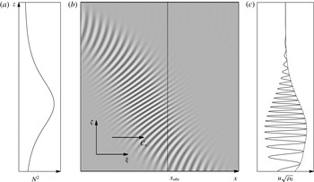
Illustration of the horizontally travelling wave solution without mean flow experiencing non-uniform stratification. (a) Squared Brunt–Väisälä frequency profile. (b) Horizontal wind component multiplied by the square root of the background density in the stationary coordinate system
 $(x,z)$
; also, the translational coordinate system
 $(\unicode[STIX]{x1D709},\unicode[STIX]{x1D701})$
that moves with the constant velocity
 $C_{x}$
to the right. (c) Profile that one would observe at
 $x_{obs}$
.
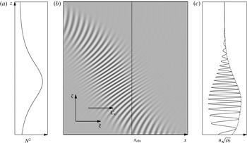
In conclusion, for this particular stratification we found an analytic travelling wave solution. It is plotted in figure 1 for some choice of
 $O(1)$
parameters and
 $G_{0}$
a bell function. This travelling wave is characterized by spatial modulation of phase as well as amplitude which is completely controlled by the stratification (see figure 1
a). The structure is that of a locally confined wave packet. For
 $\unicode[STIX]{x0394}\unicode[STIX]{x1D701}\rightarrow \infty$
the background tends to uniformity and the travelling wave merges with a plane wave. As the wave travels to the right, an observer at position
 $x_{obs}$
(see figure 1
b) would experience an upward-propagating wave packet with downward travelling wave troughs and crests. As we decided on a constant mean-flow horizontal wind, there is no shear. So, there is no energy exchange between the wave and the mean flow.
If
 $C_{x}=0$
, the result resembles a stationary wave in the original
 $(X,Z)$
coordinates. Such a wave can be interpreted as a mountain lee wave. The orography then may fix the boundary condition for
 $G_{0}$
. It is also possible to construct analytic travelling wave solutions in the same fashion, where
 $N=\text{const.}$
, corresponding to an isothermal background, and
 $u_{f0}(\unicode[STIX]{x1D701})$
is a prescribed profile. For example, choosing
 $u_{f0}(\unicode[STIX]{x1D701})=u_{0}+\unicode[STIX]{x1D6EC}\unicode[STIX]{x1D701}$
linear also provides standard antiderivatives. Here, the energy exchange rate
 $q$
is controlled by the constant shear
 $\unicode[STIX]{x1D6EC}$
. This could be used to study the energy transport due to orography in circulation models.
5.2 The isothermal, horizontally periodic travelling wave
The previous section was dedicated to the horizontally travelling wave solutions (C1) where we found exact analytic solutions to the modulation equations. This section examines case (C2), that is, the isothermal travelling wave solutions, where the local Brunt–Väisälä frequency,
 $N$
, and the logarithmic background derivative of the density,
 $\unicode[STIX]{x1D702}_{\unicode[STIX]{x1D70C}}$
, are constant. In this case a complete leading-order solution of the scaled Euler equations cannot be achieved as we did not provide the explicit evolution equation for
 $\hat{u} _{1,0}$
, which is mandatory for computing
 $\arg (A)$
in (5.6). This is because the argument in (5.13), where
 $\hat{u} _{1,0}$
disappeared in the evolution equation, does not hold since in general we allow for a non-zero vertical relative velocity,
 $C_{z}\neq 0$
. However, the remaining modulation equations are uncoupled, so they may possess some insightful solution.
Even though the fourth-order polynomial in (5.12) has an analytic solution, its calculation does not provide any further enlightenment. We differentiate (5.4) instead with respect to
 $\unicode[STIX]{x1D701}$
, which avoids lengthy terms and gives us an evolution equation for the vertical wavenumber. Closure of the system as well as substantial simplification can be gained if we restrict ourselves to horizontally periodic travelling waves, such that the horizontal derivatives in the modulation equations drop out. So, we may rewrite the modulation equations as
 $$\begin{eqnarray}\displaystyle & \displaystyle (\unicode[STIX]{x2202}_{\unicode[STIX]{x1D70F}}-C_{z}\unicode[STIX]{x2202}_{\unicode[STIX]{x1D701}})k_{z}+\unicode[STIX]{x2202}_{\unicode[STIX]{x1D701}}(\hat{\unicode[STIX]{x1D714}}+K_{x}\hat{u} _{0,0})=0, & \displaystyle\end{eqnarray}$$
 $$\begin{eqnarray}\displaystyle & \displaystyle (\unicode[STIX]{x2202}_{\unicode[STIX]{x1D70F}}-C_{z}\unicode[STIX]{x2202}_{\unicode[STIX]{x1D701}})a+(\unicode[STIX]{x2202}_{\unicode[STIX]{x1D701}}+\unicode[STIX]{x1D702}_{\unicode[STIX]{x1D70C}})(\hat{\unicode[STIX]{x1D714}}^{\prime }a)=0, & \displaystyle\end{eqnarray}$$
 $$\begin{eqnarray}\displaystyle & \displaystyle (\unicode[STIX]{x2202}_{\unicode[STIX]{x1D70F}}-C_{z}\unicode[STIX]{x2202}_{\unicode[STIX]{x1D701}})\hat{u} _{0,0}=-(\unicode[STIX]{x2202}_{\unicode[STIX]{x1D701}}+\unicode[STIX]{x1D702}_{\unicode[STIX]{x1D70C}})(\hat{\unicode[STIX]{x1D714}}^{\prime }K_{x}a). & \displaystyle\end{eqnarray}$$
The prime indicates the derivative with respect to
 $k_{z}$
, such that
 $\hat{\unicode[STIX]{x1D714}}^{\prime }(k_{z})=c_{gz}(k_{z})$
.
This system has been studied numerically by Rieper et al. (Reference Rieper, Achatz and Klein2013a ). A similar system has been investigated by Dosser & Sutherland (Reference Dosser and Sutherland2011). If we combine (5.28) with (5.29) and integrate, we obtain
 $$\begin{eqnarray}\hat{u} _{0,0}=K_{x}a+u_{0},\end{eqnarray}$$
with
 $u_{0}=u_{0}(\unicode[STIX]{x1D701}+C_{z}\unicode[STIX]{x1D70F})$
being fixed by some boundary conditions. Substituting into (5.27) gives
 $$\begin{eqnarray}\displaystyle & \displaystyle \unicode[STIX]{x2202}_{\unicode[STIX]{x1D70F}}k_{z}+\unicode[STIX]{x2202}_{\unicode[STIX]{x1D701}}(\hat{\unicode[STIX]{x1D714}}-C_{z}k_{z}+K_{x}^{2}a+K_{x}u_{0})=0, & \displaystyle\end{eqnarray}$$
 $$\begin{eqnarray}\displaystyle & \displaystyle \unicode[STIX]{x2202}_{\unicode[STIX]{x1D70F}}a+\unicode[STIX]{x2202}_{\unicode[STIX]{x1D701}}((\hat{\unicode[STIX]{x1D714}}^{\prime }-C_{z})a)=-\unicode[STIX]{x1D702}_{\unicode[STIX]{x1D70C}}\hat{\unicode[STIX]{x1D714}}^{\prime }a, & \displaystyle\end{eqnarray}$$
reducing the number of equations. As we seek stationary solutions in the translational reference frame, we drop the time derivatives and constrain
 $u_{0}=\text{const.}$
, making it some mean-flow horizontal wind offset, to get rid of its
 $\unicode[STIX]{x1D70F}$
-dependency. By that we can integrate (5.31) and solve for
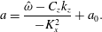 $$\begin{eqnarray}a=\frac{\hat{\unicode[STIX]{x1D714}}-C_{z}k_{z}}{-K_{x}^{2}}+a_{0}.\end{eqnarray}$$
The constant
 $a_{0}$
has absorbed
 $u_{0}$
. Hereinafter, we treat
 $a=a(k_{z})$
as function of
 $k_{z}$
, so it becomes a diagnostic quantity. Inserting it into (5.32) yields a single, nonlinear, autonomous ordinary differential equation (ODE) for
 $k_{z}$
, which can be written after some basic manipulation as
 $$\begin{eqnarray}\unicode[STIX]{x2202}_{\unicode[STIX]{x1D701}}k_{z}=f(k_{z})\quad \text{with }f(k_{z})=\frac{2\unicode[STIX]{x1D702}_{\unicode[STIX]{x1D70C}}}{K_{x}^{2}}\frac{\hat{\unicode[STIX]{x1D714}}^{\prime }(k_{z})a(k_{z})}{{a^{2}}^{\prime \prime }(k_{z})}.\end{eqnarray}$$
The denominator of
 $f$
arises after differentiating (5.33) and using the identity
 $$\begin{eqnarray}\frac{{a^{2}}^{\prime \prime }(k_{z})}{2}={a^{\prime }}^{2}(k_{z})+a(k_{z})a^{\prime \prime }(k_{z}).\end{eqnarray}$$
The ODE (5.34) has equilibrium solutions if the numerator of
 $f$
vanishes, which happens either for
 $\hat{\unicode[STIX]{x1D714}}^{\prime }(k_{z}^{-})=0$
or for
 $a(k_{z}^{+})=0$
. By definition (3.31) it turns out that
 $k_{z}^{-}=0$
. Instead of solving (5.33) for
 $k_{z}^{+}$
, which means again finding the root of a quartic function, we can use it to fix its constant
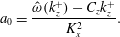 $$\begin{eqnarray}a_{0}=\frac{\hat{\unicode[STIX]{x1D714}}(k_{z}^{+})-C_{z}k_{z}^{+}}{K_{x}^{2}}.\end{eqnarray}$$
Both equilibria seem uninteresting at first glance: for
 $k_{z}^{+}$
the amplitude vanishes and for
 $k_{z}^{-}$
there is no oscillation in the vertical direction, such that wave vector is purely horizontal. But maybe there exists some solution connecting asymptotically the two equilibria, which can then be considered as asymptotic rest states, such that
 $$\begin{eqnarray}\lim _{\unicode[STIX]{x1D701}\rightarrow \pm \infty }k_{z}=k_{z}^{\pm }.\end{eqnarray}$$
Such a solution may be called a wave front. Consider, without loss of generality,
 $k_{z}^{+}<0$
and an initial condition
 $k_{z}(0)=k_{z}^{0}\in I=(k_{z}^{+},k_{z}^{-})$
. We want to settle two questions: first, for which initial condition and set of parameters does a solution exist? And second, to which of the two asymptotic rest states does the solution converge? That is, to determine the sign of
 $f$
in (5.34). As we seek upward-propagating wave packets, we shall set
 $\text{sgn}(\hat{\unicode[STIX]{x1D714}})=+1$
, such that
 $\hat{\unicode[STIX]{x1D714}}^{\prime }>0$
on
 $I$
. To guarantee that
 $|A|\in \mathbb{R}^{+}$
, we must constrain
 $a>0$
on
 $I$
. In particular, we require
 $a(k_{z}^{-})=a_{-}>0$
, which we can use to determine
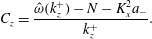 $$\begin{eqnarray}C_{z}=\frac{\hat{\unicode[STIX]{x1D714}}(k_{z}^{+})-N-K_{x}^{2}a_{-}}{k_{z}^{+}}.\end{eqnarray}$$
It emerges that
 $C_{z}>0$
, because we can estimate
 $\hat{\unicode[STIX]{x1D714}}(k_{z}^{+})<N$
for all
 $k_{z}^{+}<0$
. Our wave therefore always travels upwards. Note that by (2.18) and
 $\unicode[STIX]{x1D702}_{T}=0$
(isothermal background), we get
 $\unicode[STIX]{x1D702}_{\unicode[STIX]{x1D70C}}=-\unicode[STIX]{x1D705}^{-1}N^{2}$
. So, the numerator of
 $f$
is negative on
 $I$
. In order to obtain the sign of the denominator, we must consider (5.35) where
 $$\begin{eqnarray}a^{\prime }(k_{z})=\frac{\hat{\unicode[STIX]{x1D714}}^{\prime }(k_{z})-C_{z}}{-K_{x}^{2}}\quad \text{and}\quad a^{\prime \prime }(k_{z})=\frac{\hat{\unicode[STIX]{x1D714}}^{\prime \prime }(k_{z})}{-K_{x}^{2}}.\end{eqnarray}$$
If we evaluate (5.35) at
 $k_{z}^{-}=0$
, we find that
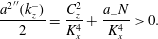 $$\begin{eqnarray}\frac{{a^{2}}^{\prime \prime }(k_{z}^{-})}{2}=\frac{C_{z}^{2}}{K_{x}^{4}}+\frac{a_{-}N}{K_{x}^{4}}>0.\end{eqnarray}$$
As the denominator must not assume a root,
 $a$
cannot have a saddle point on
 $I$
. Neither is
 $a$
allowed to exhibit a local maximum, because
 ${a^{2}}^{\prime \prime }$
would switch sign and would in particular assume a root as it is continuous. The continuity of
 $a$
prohibits also a local minimum, since it would imply a local maximum, which we have already ruled out. In conclusion,
 $a$
must not have any critical points, which yields the restriction
 $a^{\prime }>0$
on
 $I$
, i.e.
 $a$
is strictly increasing in
 $k_{z}$
. This is fulfilled regarding (5.39) if
 $\hat{\unicode[STIX]{x1D714}}^{\prime }<C_{z}$
on
 $I$
. It turns out that
 $$\begin{eqnarray}\underset{k_{z}\in I}{\text{arg}\,\text{max}}\,\hat{\unicode[STIX]{x1D714}}^{\prime }(k_{z})=\max \left(k_{z}^{+},-\frac{K_{x}}{\sqrt{2}}\right).\end{eqnarray}$$
This gives us a critical relative velocity for the existence of bounded travelling wave solutions
 $$\begin{eqnarray}C_{z}^{crit}(k_{z}^{+})=\left\{\begin{array}{@{}ll@{}}\hat{\unicode[STIX]{x1D714}}^{\prime }(-K_{x}/\sqrt{2}),\quad & \text{if }k_{z}^{+}<-K_{x}/\sqrt{2},\\ \hat{\unicode[STIX]{x1D714}}^{\prime }(k_{z}^{+}),\quad & \text{if }-K_{x}/\sqrt{2}\leqslant k_{z}^{+}<0,\end{array}\right.\end{eqnarray}$$
where
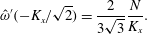 $$\begin{eqnarray}\hat{\unicode[STIX]{x1D714}}^{\prime }(-K_{x}/\sqrt{2})=\frac{2}{3\sqrt{3}}\frac{N}{K_{x}}.\end{eqnarray}$$
Demanding
 $C_{z}>C_{z}^{crit}(k_{z}^{+})$
generates by (5.38) a lower bound on
 $$\begin{eqnarray}a_{-}>a_{-}^{crit}(k_{z}^{+})=\frac{\hat{\unicode[STIX]{x1D714}}(k_{z}^{+})-k_{z}^{+}C_{z}^{crit}(k_{z}^{+})-N}{K_{x}^{2}}.\end{eqnarray}$$
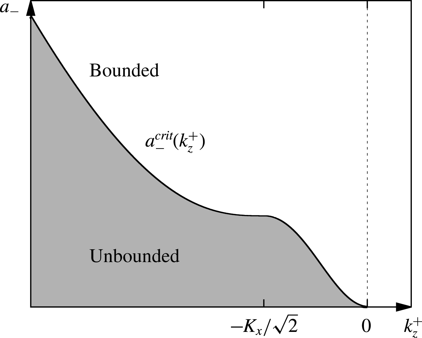
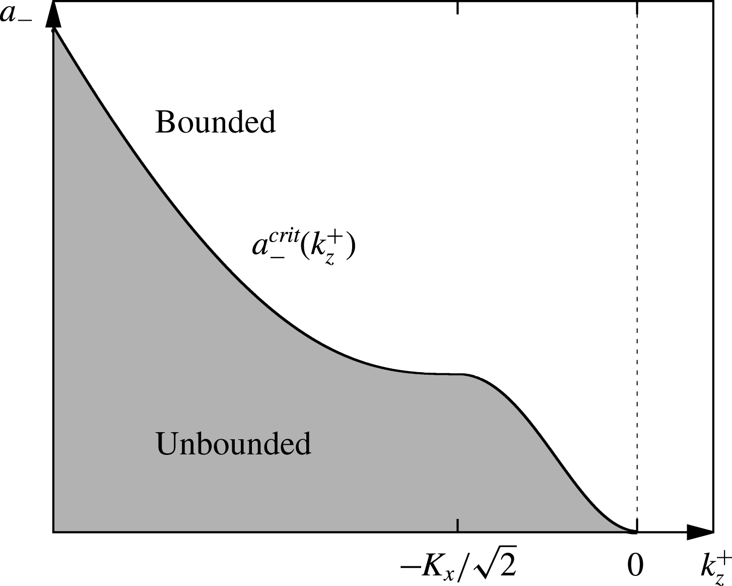
The critical asymptotic mass-specific wave action density
 $a_{-}^{crit}$
is illustrated in figure 2. Given that the previous constraints hold, by continuity
 ${a^{2}}^{\prime \prime }$
is positive on
 $I$
and the sign of
 $f$
is therefore negative. This means that for any
 $k_{z}^{0}\in I$
the solution converges to the asymptotic rest state
 $k_{z}^{+}$
as
 $\unicode[STIX]{x1D701}\rightarrow +\infty$
. Vice versa, for
 $\unicode[STIX]{x1D701}\rightarrow -\infty$
the solution tends to
 $k_{z}^{-}=0$
. So, as long as for some
 $k_{z}^{+}$
we choose
 $a_{-}$
such that it is in the white zone in figure 2, the solution converges. As soon as
 $a_{-}<a_{-}^{crit}$
(grey zone), the solution will run into a singularity and grow without bound.
Critical asymptotic mass-specific wave action density. The isothermal travelling wave solutions cannot exist if the asymptotic rest states
 $k_{z}^{+}$
and
 $a_{-}$
belong to the grey zone.
We want to point out that
 $C_{z}$
is also the vertical component of the phase velocity. Multiplying by
 $k_{z}$
therefore gives us the frequency in the stationary coordinate system. We may interpret (5.42) in terms of a critical frequency for a front-like travelling wave. In particular, for a lower boundary condition on
 $k_{z}$
, i.e. an initial condition in the stationary system, this leads to a minimal frequency for the existence of travelling wave solutions.
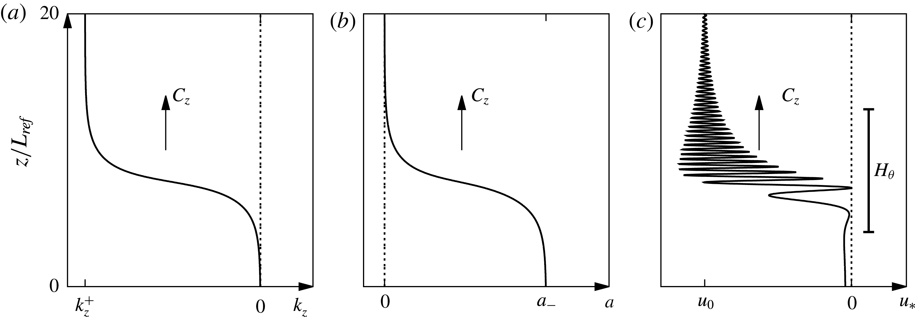
The ODE (5.34) can be solved with the explicit Euler method. For some
 $O(1)$
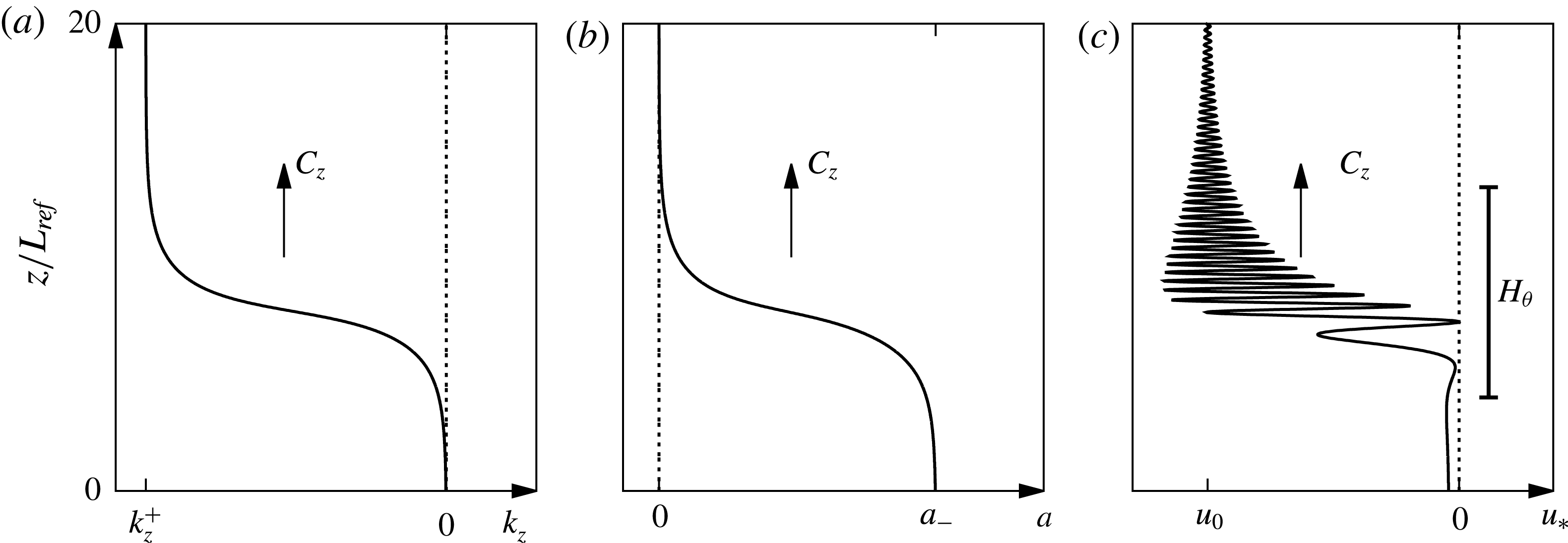
parameters (table 2) that fulfil the requirements, a particular solution illustrating the travelling wave front’s properties is plotted in figure 4. Panel (a) shows the directly computed solution of the vertical wavenumber
 $k_{z}$
, panel (b) has the mass-specific wave action density
 $a$
diagnosed from (5.33), and panel (c) displays the leading-order horizontal wind
 $$\begin{eqnarray}u_{\ast }=\hat{u} _{0,0}+(\hat{u} _{0,1}\text{e}^{\text{i}\unicode[STIX]{x1D6F7}\unicode[STIX]{x1D700}^{-1}}+\text{c.c.}),\end{eqnarray}$$
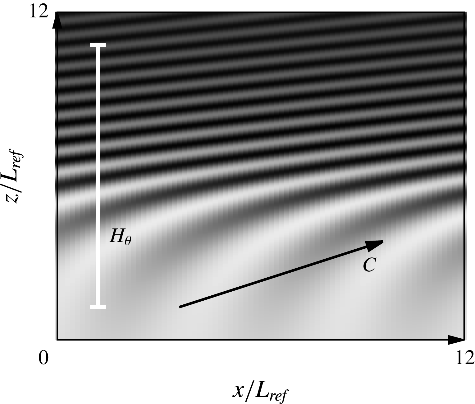
which is also shown in figure 3 from a two-dimensional perspective. We chose
 $u_{0}=-K_{x}a_{-}$
for (5.30), so the mean-flow horizontal wind drops to zero after the front has propagated through. To compute
 $\unicode[STIX]{x1D6F7}$
from (5.11), we applied the very same Euler method. To compute
 $\hat{u} _{0,1}$
according to (3.24), we set
 $\arg (A)=\text{const.}$
because we lack an equation for it. The error produced by this oversimplification occurs in the wake of the front when
 $k_{z}$
tends to zero, such that the slow phase
 $\arg (A)$
becomes vertically dominant and maybe produces some long-wavelength vertical oscillation. From the two-dimensional point of view, the leading term in
 $\unicode[STIX]{x1D6F7}$
is then still
 $K_{x}\unicode[STIX]{x1D709}$
. However, this will not change the overall picture as the induced mean-flow regarding (5.30) is not affected by the slow phase. Again this travelling wave is characterized by spatial modulation of amplitude as well as phase.
Illustration of the isothermal travelling wave front in two dimensions propagating with velocity
 $\boldsymbol{C}$
. Horizontal wind
 $u_{\ast }$
is as given by (5.45); the potential temperature scale height
 $H_{\unicode[STIX]{x1D703}}$
is shown for comparison.
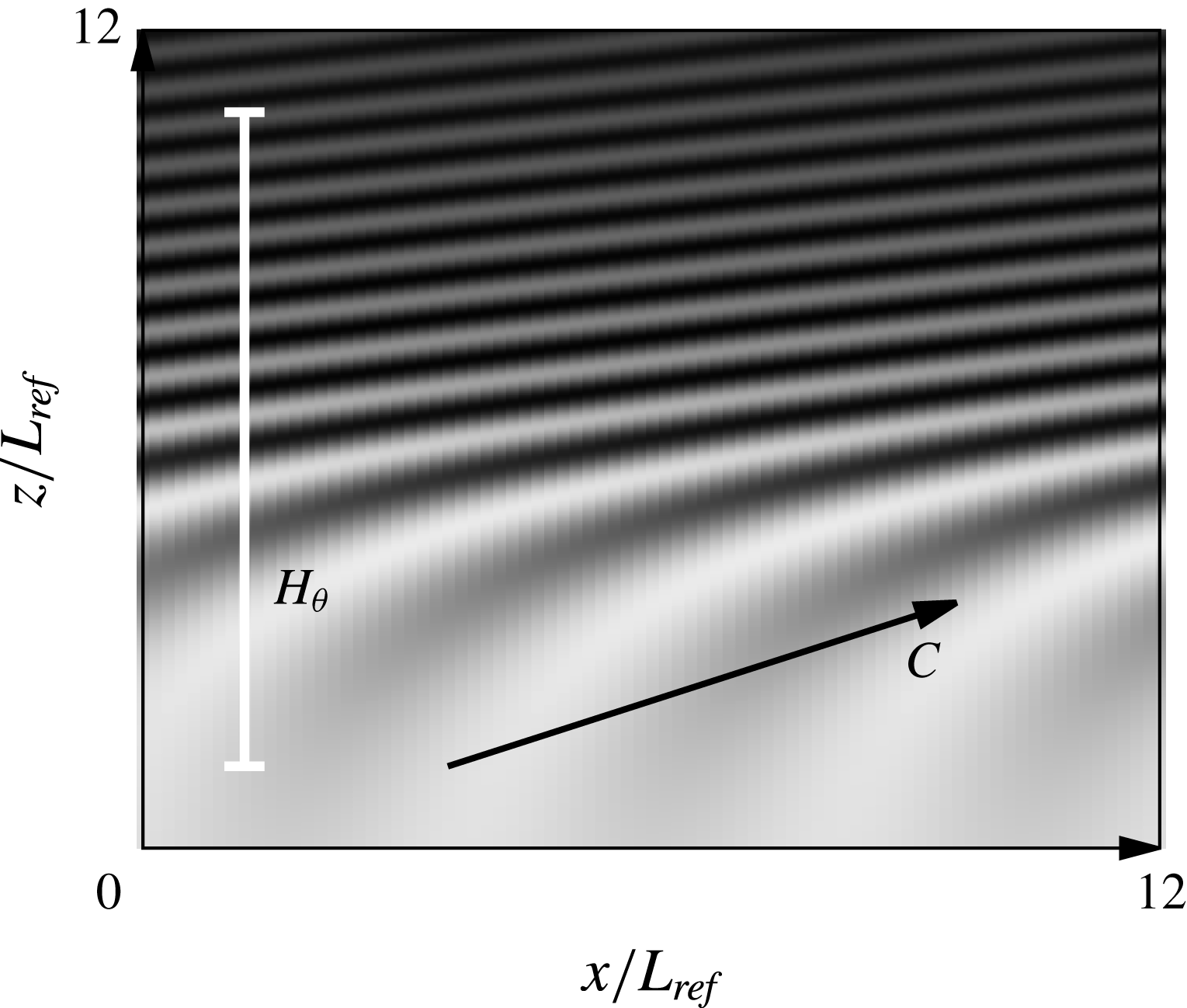
Illustration of the isothermal travelling wave front in one dimension. (a) Vertical wavenumber. (b) Mass-specific wave action density. (c) Horizontal wind as given by (5.45) and the potential temperature scale height
 $H_{\unicode[STIX]{x1D703}}$
for comparison.
 $O(1)$
parameters defining an isothermal, horizontally periodic travelling wave.

The mass-specific wave action density and therefore the amplitude remain constant in the wake of the front. So, at first glance, it seems that the wave induces wave energy into the mean flow. Because one would usually expect increasing amplitude with height due to the thinning air when the wave propagates upwards and due to the fact that the wave energy scales with the background density, this ‘extra’ energy should then accelerate the mean flow. This interpretation turns out to be incorrect, which becomes clear if we compute the wave–mean-flow energy exchange rate from § 4 in the stationary (
 $X,Z$
) coordinate system,
 $$\begin{eqnarray}q=K_{x}^{2}\unicode[STIX]{x1D70C}_{0}a(k_{z})\hat{\unicode[STIX]{x1D714}}^{\prime }(k_{z})a^{\prime }(k_{z})\unicode[STIX]{x2202}_{Z}k_{z}<0.\end{eqnarray}$$
Here, we used (5.30) and the estimates from this section. We can already conclude that energy is exchanged directly in the front where the gradient is located. The rate is always negative. On the other hand, the wave gains energy from the mean flow and the mean-flow horizontal wind decelerates. This surprising behaviour is demystified if we consider also the wave energy flux from (4.1). It tells us that the wave energy is transported with the group velocity
 $\hat{\unicode[STIX]{x1D714}}^{\prime }$
. But the front moves with
 $C_{z}$
, which is always greater than
 $\hat{\unicode[STIX]{x1D714}}^{\prime }$
as we suppressed any critical points for
 $a$
.
In summary, the fast travelling wave front can only be sustained if it obtains energy from the mean flow. One may ask if inverted travelling wave fronts could exist as solutions to the isothermal, horizontally periodic modulation equations. These would be solutions where the asymptotic rest states switched. So,
 $k_{z}^{-}\neq 0$
and
 $a_{-}=0$
but
 $k_{z}^{+}=0$
and
 $a_{+}\neq 0$
. These solutions would be referred to as travelling wave backs. It turns out that backs cannot be solutions under any circumstances. We state this claim here unproved as the argumentation goes beyond the scope of this survey.
6 Numerical validation of the travelling wave solutions under the full Euler dynamics
In the previous sections we found that travelling wave solutions for the modulation equations appear in two distinct cases. For the first case (C1), when the atmosphere is non-uniformly stratified, we were able to derive exact analytic solutions. The wave vectors can point in any direction but vertical, though the entire wave travels only in the horizontal direction. For the second case (C2), when the atmosphere is uniformly stratified (isothermal), we managed to show existence and the structure of the travelling wave solutions: assuming horizontal periodicity it turns out to be a front-like solution. These travelling waves propagate both horizontally and vertically. We found exact solutions to the modulation equations; they are, however, asymptotic solutions to the fully nonlinear Euler equations. In this section we want to test the consistency of these solutions. The travelling wave solutions in the (C1) case will be challenged numerically, so we can check the range of validity as the travelling wave solutions could be unstable intrinsically or only be sustained for very small, even unrealistic
 $\unicode[STIX]{x1D700}$
. For this purpose, we will use a conservative solver of the Euler equations, the pincFloit model.
PincFloit stands for pseudo-incompressible flow solver with implicit turbulence and was introduced by Rieper, Hickel & Achatz (Reference Rieper, Hickel and Achatz2013b ). This finite-volume flow solver conserves energy, momentum and mass and therefore suits the purpose well. Within the framework of the model it is possible to simulate with almost unconstrained background stratifications apart from the uniform, weakly stratified atmosphere. The fidelity of the model was tested against standard cases. Rieper et al. (Reference Rieper, Achatz and Klein2013a ) applied pincFloit to check the range of validity of the extended WKB theory for the gravity waves of Achatz et al. (Reference Achatz, Klein and Senf2010), which provides the basis for our travelling wave solutions. Recently, Muraschko et al. (Reference Muraschko, Fruman, Achatz, Hickel and Toledo2015) and Bölöni et al. (Reference Bölöni, Ribstein, Muraschko, Sgoff, Wei and Achatz2016) derived a numerical solver for the modulation equations based on a Lagrangian ray-tracing approach for horizontally homogeneous GW packets that was also tested with the aid of pincFloit. It discretizes the governing equations on an equidistant staggered C-grid. From the alternative schemes that the model provides, it proved practical to apply the third-order, low-storage Runge–Kutta time-stepping scheme, which is total variation diminishing. This is combined with the MUSCL scheme for spatial discretization and a monotonized central flux limiter. As the name of the model implies, it is capable of solving the compressible Navier–Stokes equations. But since this survey is only interested in the Euler equations, any diffusion or dissipation was switched off.
Fixed parameters that define the travelling wave and experimental set-up.

We validate the (C1) travelling wave solution with non-uniform stratification as given by the equations (5.22)–(5.26). They are not compactly supported on the two-dimensional domain. Inevitably, the wave will touch the boundary of the computational domain. In order to prevent reflection, we prescribe the analytic solution on the boundary cells for all times. We choose a particularly challenging test case such that the background stratification and the amplitude varies like
 $O(1)$
on the whole domain. The mean-flow horizontal wind is chosen in such a way that the horizontal translational relative velocity
 $C_{x}$
vanishes, so
 $$\begin{eqnarray}U_{f}=-N_{min}/K_{x}.\end{eqnarray}$$
By this choice the travelling wave is stationary in the fixed coordinate system, such that
 $(\unicode[STIX]{x1D709},\unicode[STIX]{x1D701})=(X,Z)$
, which makes it convenient to compare the initial condition with the final state. The wave amplitude is set to be of the same order as the mean flow to provoke nonlinear coupling. So, the set-up can be viewed as a wave that inherently wants to migrate towards the right side with a constant horizontal group velocity but faces an opposing wind of the exact same velocity. If the model manages to balance these tendencies, the outcome stands at rest.
The parameters that define the travelling wave and the background are presented in table 3. They were chosen in such a way that they resemble a typically unresolved wave in weather and climate models. Here,
 $l_{x}$
and
 $l_{z}$
are the domain sizes in
 $x$
- and
 $z$
-directions, respectively. The initial wave action flux is given by a bell-shaped function
 $$\begin{eqnarray}G(X,Z)=G_{max}\left(1+\left(\frac{\unicode[STIX]{x1D6F9}(X,Z)-\unicode[STIX]{x1D6F9}(X_{pos},Z_{pos})}{\unicode[STIX]{x0394}\unicode[STIX]{x1D6F9}}\right)^{4}\right)^{-2},\end{eqnarray}$$
where
 $G_{max}$
is the maximum flux at the peak.
To prescribe the stratification in the model, we have to provide the background density, Exner pressure and potential temperature. The latter can be computed by means of standard antiderivatives from (5.23). The background Exner pressure is defined through the hydrostatic equation (2.13), which we must integrate numerically. This is achieved by a simple Euler forward scheme with very high resolution. It looks costly at first glance but only needs to be computed once at the start.
Deviations between simulation and theory are measured by the weighted norms of the numerically simulated field (num) minus the analytically expected (true) field. Hereinafter, we consider the horizontal wind field as we did not find any significant differences from the other fields in terms of errors. We define the weighted error norms as
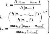 $$\begin{eqnarray}\left.\begin{array}{@{}c@{}}\displaystyle l_{1}=\frac{I(|u_{true}-u_{num}|)}{I(|u_{true}|)}\\ \displaystyle l_{2}=\left(\frac{I(|u_{true}-u_{num}|^{2})}{I(|u_{true}|^{2})}\right)^{1/2}\\ \displaystyle l_{\infty }=\frac{\max _{x,z}(|u_{true}-u_{num}|)}{\max _{x,z}(|u_{true}|)},\end{array}\right\}\end{eqnarray}$$
where
 $I$
denotes the numerical approximation to the integral
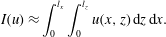 $$\begin{eqnarray}I(u)\approx \int _{0}^{l_{x}}\int _{0}^{l_{z}}u(x,z)\,\text{d}z\,\text{d}x.\end{eqnarray}$$
The numerical quadrature exploits the trapezoidal rule.
In order to test the consistency of the travelling wave solutions, the scale separation parameter
 $\unicode[STIX]{x1D700}$
is altered while all other parameters, as given in table 3 determining the properties of the travelling wave, are kept constant. The analytical asymptotic solution in non-dimensional form can be written as
 $$\begin{eqnarray}U_{true}=\hat{U} _{0,0}+(\hat{U} _{0,1}\text{e}^{\text{i}\unicode[STIX]{x1D700}^{-1}\unicode[STIX]{x1D6F7}}+\text{c.c.})+O(\unicode[STIX]{x1D700})\end{eqnarray}$$
for
 $\unicode[STIX]{x1D700}\rightarrow 0$
and
 $(X,Z,T)$
fixed. We call the solution consistent if we can reproduce the analytically expected order of convergence from (3.1) of
 $M=1$
numerically for a broad range of
 $\unicode[STIX]{x1D700}$
. In § 2 we defined
 $$\begin{eqnarray}\unicode[STIX]{x1D700}=\frac{L_{ref}}{H_{\unicode[STIX]{x1D703}}}.\end{eqnarray}$$
As we vary
 $\unicode[STIX]{x1D700}$
, we keep
 $L_{ref}$
fixed, such that the spatial resolution per wave period remains constant. This choice provides the benefit that we do not need to adapt the resolution for each value of
 $\unicode[STIX]{x1D700}$
. If we did so, then we could not distinguish effects on the error of the varying
 $\unicode[STIX]{x1D700}$
from the varying resolution. All experiments were performed with a resolution of
 $256\times 512$
grid cells, which corresponds to approximately 18 grid cells per wave period, which is a reasonable value to resolve all important features.
As we change
 $\unicode[STIX]{x1D700}$
from one experiment to another, we must constrain that
 $T=\unicode[STIX]{x1D700}t=O(1)$
, which fulfils a necessary condition of the asymptotic ansatz, and hence the dimensionful overall simulation time must change like
 $$\begin{eqnarray}t_{end}^{\ast }=O\left(\frac{t_{ref}}{\unicode[STIX]{x1D700}}\right)=O(\unicode[STIX]{x1D700}^{-2/3})\quad \text{since }t_{ref}=\sqrt{H_{\unicode[STIX]{x1D703}}/g}=O(\unicode[STIX]{x1D700}^{-1/2}).\end{eqnarray}$$
Table 4 presents the parameters defining each of the five experiments. In particular, the simulation time
 $t_{end}^{\ast }$
is shown in the rightmost column. The potential temperature scale height varies from approximately 20 to 46 km throughout the simulations, which gives us a considerable range for the scale separation.
Varying parameters for the experiments testing the consistency of the travelling wave.
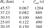
Computational corroboration of the existence of horizontally travelling wave solutions. (a,d,g) Stratification represented by the local squared Brunt–Väisälä frequency. (b,e,h) Initial total horizontal wind
 $u_{true}$
in
 $\text{m}~\text{s}^{-1}$
. (c,f,i) Deviation between the numerical and the approximate asymptotic solutions after simulation time
 $t_{end}^{\ast }$
(see table 4), i.e.
 $u_{true}-u_{num}$
. In (h) the filled white curve depicts a streamline being inflated by a factor 64.

The simulation results are plotted in figure 5. The stratification, the horizontal wind and its relative deviation from the analytic solution are depicted for three of the experiments. For smallest
 $\unicode[STIX]{x1D700}=0.067$
(a–c) the stratification is moderate and the amplitude envelope, which is given by the wave action flux
 $G$
, is also rather broad in width. The horizontal wind oscillates around a mean flow of approximately
 $12~\text{m}~\text{s}^{-1}$
with an amplitude of
 $3~\text{m}~\text{s}^{-1}$
.
The lines of constant phase are nearly straight, and so are the characteristic lines
 $\unicode[STIX]{x1D6F9}$
, which define the shape of the envelope. With even smaller
 $\unicode[STIX]{x1D700}$
the wave will get closer to the uniformly stratified regime with infinitesimal amplitude which can be captured by the Boussinesq theory. The relative error after the simulation is, as expected, very small, much less than 1 % at the peaks. Remarkably, the error is almost perfectly in phase with the initial wave, at least in the middle of the domain. This means that errors are not generated by non-stationary effects. The wave does not move at all, and the peaks are slightly smeared out, probably by some numerical dissipation. By increasing
 $\unicode[STIX]{x1D700}$
, the width of the stratification peak narrows. Also, the envelope confines and its maximum increases. The mean-flow horizontal wind gets stronger and we can expect nonlinear effects.
For
 $\unicode[STIX]{x1D700}=0.1$
(figure 5
d–f) the mean flow approaches
 $15~\text{m}~\text{s}^{-1}$
and the horizontal wind varies with an amplitude of approximately
 $\pm 10~\text{m}~\text{s}^{-1}$
, which produces substantial shear. In this case, we observe clearly some error sources at the upper boundary. These are numerical errors. As we prescribe the expected analytic solution at the boundaries, even small deviations of the numerical solution in the domain can cause discontinuities directly at the boundary. These shocks then propagate into the domain.
For even higher
 $\unicode[STIX]{x1D700}$
, nonlinear effects start to dominate the error production. In the experiment where
 $\unicode[STIX]{x1D700}=0.15$
(figure 5
g–i), the mean flow is approximately
 $18~\text{m}~\text{s}^{-1}$
and the horizontal wind oscillates with an amplitude of approximately
 $40~\text{m}~\text{s}^{-1}$
, which is not captured by the colour scale of figure 5. Here, we find some quadrupole structure in the relative error field that indicates phase shifts by some instability process which are triggered most likely by the boundary discontinuities. The local error exceeds
 $3~\text{m}~\text{s}^{-1}$
at some points.
For this particular case we also plotted a streamline in figure 5(h) which is amplified for better visibility. This line represents just as well a mountain ridge of about 200 m height that could have excited the wave.
Convergence of the error norms with regard to
 $\unicode[STIX]{x1D700}$
: (solid line) linear regression on a log–log scale with the least squares method reveals an order of convergence
 $M$
and its standard deviation; (long dashed) first-order, (medium dashed) second-order and (short dashed) third-order lines.
For all five experiments, we computed the error norms according to (6.3). The results are shown in figure 6 where we have plotted the error norms against
 $\unicode[STIX]{x1D700}$
on a log–log scale. A least squares fit gives us the order of convergence
 $M$
assuming that the error norms converge like
 $$\begin{eqnarray}l_{n}=C\unicode[STIX]{x1D700}^{M}\quad \text{for }n=1,2,\infty .\end{eqnarray}$$
We also computed its standard deviation, depicted alongside the fitted lines in figure 6. For all three norms we obtain convergence like
 $O(\unicode[STIX]{x1D700}^{3})$
. Even after subtracting the rounded error margin of 1 from the order, it is apparently still included in the expected
 $O(\unicode[STIX]{x1D700})$
-convergence with a comfortable cushion. For larger
 $\unicode[STIX]{x1D700}$
the model probably overestimates the norms due to the numerical errors at the boundaries propagating into the domain and triggering instabilities. We tested the influence of this effect by changing the integration domain of the norms as follows:
 $$\begin{eqnarray}I(u)\approx \int _{\unicode[STIX]{x1D6FF}}^{l_{x}-\unicode[STIX]{x1D6FF}}\int _{\unicode[STIX]{x1D6FF}}^{l_{z}-\unicode[STIX]{x1D6FF}}u(x,z)\,\text{d}z\,\text{d}x\end{eqnarray}$$
with
 $\unicode[STIX]{x1D6FF}$
some positive fixed number. So, we focus on a smaller box and ignore cells that are potentially influenced by the boundaries. For some values of
 $\unicode[STIX]{x1D6FF}$
we recalculated the error norms for every
 $\unicode[STIX]{x1D700}$
. There was no significant effect on the order of convergence. So either the hypothesis of boundary discontinuities propagating into the domain causing instabilities is wrong, or they already contaminate the whole domain after the simulation time as they propagate faster than expected, or instabilities are excited by other processes. This remains an open question.
However, for small
 $\unicode[STIX]{x1D700}$
the norms are presumably also overrated as the amplitudes become so small that nonlinear coupling between the wave and the mean flow becomes inefficient and numerical damping takes over. Taking these effects into account, with an order of convergence of about three, we can safely conclude that the travelling waves are consistent for a significant parameter range.
7 Hydrostatic gravity waves
In the previous section, we showed that the horizontally travelling wave solutions (C1) resemble stationary mountain lee waves at least qualitatively. In the numerical experiments, though, we used rather small wavelengths of approximately 3 km in both vertical and horizontal directions. As the overall motivation of this survey is to lay the foundation for more realistic instability criteria in gravity wave parametrizations, the natural choice to test the asymptotic consistency of the travelling wave solutions was to use typically unresolved small wavelengths. But mountain waves in nature are mostly hydrostatic waves, i.e. they exhibit much longer horizontal than vertical wavelengths, such that their dynamics is anisotropic. For the derivation of the modulation equations we assumed a non-hydrostatic, isotropic scaling. This section is concerned with the question of whether our modulation equations and their travelling wave solutions still apply in the hydrostatic limit.
In this regard Achatz et al. (Reference Achatz, Klein and Senf2010, Reference Achatz, Ribstein, Senf and Klein2017) showed that the consistency between the scale asymptotics of the Euler equations and the pseudo-incompressible equations also holds for hydrostatic gravity waves. Bölöni et al. (Reference Bölöni, Ribstein, Muraschko, Sgoff, Wei and Achatz2016) investigated the non-hydrostatic modulation equations numerically by applying a ray-tracer method. The model was validated, among others, by initializing hydrostatic waves with a horizontal-to-vertical wavelength ratio of 10. The results were compared with reference simulations computed with pincFloit (Rieper et al. Reference Rieper, Hickel and Achatz2013b ). Both models were in excellent agreement.
Based on these considerations we will rescale the Euler equations (2.19) for hydrostatic gravity waves and solve them asymptotically with the spectral WKB method presented in § 3. We assume the horizontal-to-vertical wavelength ratio to be
 $O(\unicode[STIX]{x1D700})$
whereas the same distinguished limit provided in § 2 shall hold. In particular, the vertical wavelength is small in comparison to the scale height and the background varies slowly with respect to the fast oscillations. In order to capture the anisotropic dynamics, we introduce rescaled coordinates
 $$\begin{eqnarray}(X,Z,T)=(\unicode[STIX]{x1D700}^{2}x,\unicode[STIX]{x1D700}z,\unicode[STIX]{x1D700}^{2}t)\end{eqnarray}$$
and consider the following ansatz for the WKB approximation:
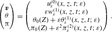 $$\begin{eqnarray}\displaystyle \left(\begin{array}{@{}c@{}}\boldsymbol{v}\\ \unicode[STIX]{x1D703}\\ \unicode[STIX]{x03C0}\end{array}\right)=\left(\begin{array}{@{}c@{}}u_{\unicode[STIX]{x1D700}}^{(0)}(x,z,t;\unicode[STIX]{x1D700})\\ \unicode[STIX]{x1D700}w_{\unicode[STIX]{x1D700}}^{(1)}(x,z,t;\unicode[STIX]{x1D700})\\ \unicode[STIX]{x1D703}_{0}(Z)+\unicode[STIX]{x1D700}\unicode[STIX]{x1D703}_{\unicode[STIX]{x1D700}}^{(1)}(x,z,t;\unicode[STIX]{x1D700})\\ \unicode[STIX]{x1D70B}_{0}(Z)+\unicode[STIX]{x1D700}^{2}\unicode[STIX]{x1D70B}_{\unicode[STIX]{x1D700}}^{(2)}(x,z,t;\unicode[STIX]{x1D700})\end{array}\right). & & \displaystyle\end{eqnarray}$$
Note that, in contrast to (7.2), the vertical wind occurs at
 $O(\unicode[STIX]{x1D700})$
(cf. Achatz et al.
Reference Achatz, Klein and Senf2010) while all the other symbols have their usual meaning. If we insert (7.2) into the Euler equations (2.1) and substitute by
 $$\begin{eqnarray}\boldsymbol{U}=(u,w,B,P)^{\text{T}}:=\left(u_{\unicode[STIX]{x1D700}}^{(0)},\unicode[STIX]{x1D700}w_{\unicode[STIX]{x1D700}}^{(1)},\frac{1}{N}\frac{\unicode[STIX]{x1D703}_{\unicode[STIX]{x1D700}}^{(1)}}{\unicode[STIX]{x1D703}_{0}},\unicode[STIX]{x1D703}_{0}\unicode[STIX]{x1D70B}_{\unicode[STIX]{x1D700}}^{(2)}\right)^{\text{T}},\end{eqnarray}$$
then we can exploit the series expansion (3.1) combined with the WKB assumption
 $$\begin{eqnarray}(X,Z,T)\mapsto \hat{U} _{n,m}(X,Z,T),\;\unicode[STIX]{x1D6F7}(X,Z,T).\end{eqnarray}$$
By the weak asymptotic approach of appendix A we can order terms in powers of
 $\unicode[STIX]{x1D700}$
and thereby obtain to leading order a homogenous linear system for the primary harmonics
 $\unicode[STIX]{x1D648}\hat{U} _{0,1}=0$
with the coefficient matrix
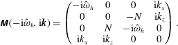 $$\begin{eqnarray}\unicode[STIX]{x1D648}(-\text{i}\hat{\unicode[STIX]{x1D714}}_{h},\text{i}\boldsymbol{k})=\left(\begin{array}{@{}cccc@{}}-\text{i}\hat{\unicode[STIX]{x1D714}}_{h} & 0 & 0 & \text{i}k_{x}\\ 0 & 0 & -N & \text{i}k_{z}\\ 0 & N & -\text{i}\hat{\unicode[STIX]{x1D714}}_{h} & 0\\ \text{i}k_{x} & \text{i}k_{z} & 0 & 0\end{array}\right).\end{eqnarray}$$
The intrinsic frequency for the hydrostatic waves is found to be
 $\hat{\unicode[STIX]{x1D714}}_{h}=\unicode[STIX]{x1D714}-k_{x}\hat{u} _{0,0}$
where
 $\unicode[STIX]{x1D714}$
and
 $\boldsymbol{k}$
are the time and spatial derivatives of the phase
 $\unicode[STIX]{x1D6F7}$
, respectively. The homogenous system for
 $\hat{U} _{0,1}$
has non-trivial solution only if
 $\det (\unicode[STIX]{x1D648}(-\text{i}\hat{\unicode[STIX]{x1D714}}_{h},\text{i}\boldsymbol{k}))=0$
, which yields the dispersion relation
 $$\begin{eqnarray}\hat{\unicode[STIX]{x1D714}}_{h}^{2}=\frac{N^{2}k_{x}^{2}}{k_{z}^{2}}.\end{eqnarray}$$
The kernel of
 $\unicode[STIX]{x1D648}$
provides the polarization relation
 ${\mathcal{U}}\in \ker (\unicode[STIX]{x1D648})$
, which turns out to be the same as the non-hydrostatic (3.23), so that the solution can be written as
 $$\begin{eqnarray}\hat{U} _{0,1}=A{\mathcal{U}}(\hat{\unicode[STIX]{x1D714}}_{h},\boldsymbol{k}),\end{eqnarray}$$
with
 $A\in \mathbb{C}$
being the scalar amplitude. To leading order, we also get constraints for the mean flow:
 $$\begin{eqnarray}{\hat{w}}_{0,0}=0,\quad \hat{B}_{0,0}=0\quad \text{and}\quad \unicode[STIX]{x2202}_{X}\hat{u} _{0,0}=0.\end{eqnarray}$$
At the next order, we obtain an inhomogeneous system for the primary harmonics of the same form as (3.17) with only a change in the linear differential operator,
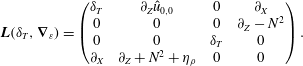 $$\begin{eqnarray}\boldsymbol{L}(\unicode[STIX]{x1D6FF}_{T},\unicode[STIX]{x1D735}_{\unicode[STIX]{x1D700}})=\left(\begin{array}{@{}cccc@{}}\unicode[STIX]{x1D6FF}_{T} & \unicode[STIX]{x2202}_{Z}\hat{u} _{0,0} & 0 & \unicode[STIX]{x2202}_{X}\\ 0 & 0 & 0 & \unicode[STIX]{x2202}_{Z}-N^{2}\\ 0 & 0 & \unicode[STIX]{x1D6FF}_{T} & 0\\ \unicode[STIX]{x2202}_{X} & \unicode[STIX]{x2202}_{Z}+N^{2}+\unicode[STIX]{x1D702}_{\unicode[STIX]{x1D70C}} & 0 & 0\end{array}\right).\end{eqnarray}$$
Multiplying the inhomogeneous equation from the left by the conjugate transpose of the kernel vector and adding its complex conjugate, we obtain a conservation law
 $$\begin{eqnarray}\unicode[STIX]{x2202}_{T}{\mathcal{A}}+\unicode[STIX]{x1D735}_{\unicode[STIX]{x1D700}}\boldsymbol{\cdot }(\boldsymbol{c}_{gh}{\mathcal{A}})=0\end{eqnarray}$$
for the wave action density
 ${\mathcal{A}}=\unicode[STIX]{x1D70C}_{0}|A|^{2}/\hat{\unicode[STIX]{x1D714}}_{h}$
, which constitutes an equation of motion for the absolute wave amplitude
 $|A|$
. By subtracting its complex conjugate, we get an equation of motion for the argument of the amplitude,
 $$\begin{eqnarray}(\unicode[STIX]{x2202}_{T}+\boldsymbol{c}_{gh}\boldsymbol{\cdot }\unicode[STIX]{x1D735}_{\unicode[STIX]{x1D700}})\arg (A)=-k_{x}\hat{u} _{1,0}.\end{eqnarray}$$
The hydrostatic group velocity is given by
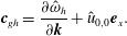 $$\begin{eqnarray}\boldsymbol{c}_{gh}=\frac{\unicode[STIX]{x2202}\hat{\unicode[STIX]{x1D714}}_{h}}{\unicode[STIX]{x2202}\boldsymbol{k}}+\hat{u} _{0,0}\boldsymbol{e}_{x}.\end{eqnarray}$$
Also at the next order, we find the very same equation of motion for the non-hydrostatic mean-flow horizontal wind (3.34), which can be recast with the aid of the hydrostatic polarization (7.7) as
 $$\begin{eqnarray}\unicode[STIX]{x1D70C}_{0}(\unicode[STIX]{x2202}_{T}\hat{u} _{0,0}+\unicode[STIX]{x2202}_{X}\hat{P}_{0,0})=-\unicode[STIX]{x1D735}_{\unicode[STIX]{x1D700}}\boldsymbol{\cdot }((\boldsymbol{c}_{gh}-\hat{u} _{0,0}\boldsymbol{e}_{x})k_{x}{\mathcal{A}}).\end{eqnarray}$$
In conclusion, we find hydrostatic modulation equations (7.10), (7.11) and (7.13), which differ from the non-hydrostatic ones (3.32), (3.33) and (3.38) only in the dispersion relation (7.6). If we perform a Taylor expansion of the non-hydrostatic dispersion relation (3.22) for
 $|k_{x}|\ll |k_{z}|$
in the variable
 $k_{x}/k_{z}$
, i.e. assuming steep wave vectors (Bühler Reference Bühler2009, p. 121), we obtain
 $$\begin{eqnarray}\hat{\unicode[STIX]{x1D714}}=\hat{\unicode[STIX]{x1D714}}_{h}+O(|k_{x}/k_{z}|^{2}).\end{eqnarray}$$
Therefore, we deduce that the non-hydrostatic modulation equations also hold in the hydrostatic limit. This statement also implies that the travelling wave solutions, which we found for the non-hydrostatic case, are equally valid for large horizontal wavelength or small
 $K_{x}$
, accordingly. The result is of particular interest for the (C1) class since it demonstrates that these solutions indeed describe typical mountain lee waves.
8 Conclusion
We started our derivations from the dimensionless, fully compressible Euler equations. By assuming low Mach number, leading-order stable stratification, non-hydrostatic motion and a large internal Froude number, we found a distinguished limit similar to that in Achatz et al. (Reference Achatz, Klein and Senf2010). The scale separation parameter
 $\unicode[STIX]{x1D700}$
, which is now the only parameter appearing in the equations, is the ratio of the dominant wavelength to the scale height.
The scaled Euler equations were derived from a multiple-scale ansatz that divided the wave from a hydrostatic background. We combined a spectral expansion approach with the WKB assumption of slow modulation of amplitude and phase. So, the frequency and wavenumbers are defined locally as the temporal and spatial derivatives of the phase, respectively. Since the system is nonlinear and we allowed for wave–mean-flow interaction, even the leading-order equations are contaminated by higher harmonics.
Instead of an averaging technique (e.g. Grimshaw Reference Grimshaw1974; Tabaei & Akylas Reference Tabaei and Akylas2007) that assumes a priori periodicity of the asymptotic solution with respect to the fast phase, we applied the more general approach presented in Danilov et al. (Reference Danilov, Omelyanov, Shelkovich and Karasev2003) of weak asymptotic solutions.
Investigating the results of the asymptotic analysis leads to the modulation equations: equations of motion for the phase, wave action density and leading-order mean-flow variables. These equations are in line with the findings of Achatz et al. (Reference Achatz, Klein and Senf2010). But in addition we found an evolution equation for the argument of the complex-valued amplitude and a constraint for the higher-order mean-flow horizontal wind which becomes necessary to close the equation system. Computing the energy budget revealed that these equations conserve the sum of wave and mean-flow energy.
We found two distinct classes of travelling wave solutions for the modulation equations: the horizontally travelling wave solution and the isothermal travelling wave solution. For the former, we were able to construct analytic solutions. The horizontally travelling wave solution with
 $C_{x}=0$
may be applied to model mountain lee waves for arbitrary stratification, background horizontal wind and orography. Typically, mountain lee waves are hydrostatic. Although the modulation equations were derived for non-hydrostatic gravity waves, it was shown that they also hold in the hydrostatic limit where the wave vector becomes steep. With the additional assumption that the wave is horizontally periodic, we investigated the existence and the shape of the isothermal travelling wave solution. It resembles an upward-propagating wave front. Quite surprisingly, the isothermal travelling wave front decelerates the mean flow in order to sustain its constant amplitude.
The horizontally travelling waves were validated numerically against the fully nonlinear Euler equations. Exact solutions of the modulation equations fulfil the Euler dynamics asymptotically. The purpose of the numerical simulations was to clarify the consistency of the solutions, i.e. range of validity of the asymptotic approximation. The travelling wave solutions performed surprisingly well: they exceeded the analytically expected order of convergence of one as the scale separation parameter tends to zero. The numerically computed order turned out to be around three. This result holds over a broad range of scale separation parameters, which proves the consistency of the travelling wave solutions presented in this survey.
In a companion paper we will analyse the travelling waves that we found here, with respect to stability, by analytical and numerical methods.
Acknowledgements
The authors thank the German Research Foundation (DFG) for partial support through the research unit Multiscale Dynamics of Gravity Waves (MS-GWaves) and through grants AC 71/8-1, AC 71/9-1, AC 71/10-1 and KL 611/25-1. M.S. thanks G. Bölöni for vital support with pincFloit.
Appendix A
This appendix introduces the weak asymptotic scheme which allows us to successively iterate the asymptotic solution in order to achieve an equation hierarchy. Our objective is to establish that the coefficients
 ${\mathcal{C}}_{k,l}$
from (3.7) vanish independently of
 $k$
and
 $l$
. This is usually achieved by an orthogonality argument that the harmonics are mutually orthogonal with respect to the inner product given by the average over the interval
 $[0,2\unicode[STIX]{x03C0}]$
with respect to the fast phase
 $\unicode[STIX]{x1D700}^{-1}\unicode[STIX]{x1D6F7}$
(Miura & Kruskal Reference Miura and Kruskal1974; Grimshaw Reference Grimshaw1974; Tabaei & Akylas Reference Tabaei and Akylas2007). There are two issues with this approach: first, the fast phase does depend on
 $\unicode[STIX]{x1D700}$
, such that the phase lines squeeze together when
 $\unicode[STIX]{x1D700}$
tends to zero. Second and most importantly,
 $\unicode[STIX]{x1D6F7}$
is actually a function of space and time, so solving the integral requires an integration by substitution. We can circumvent these issues if we seek asymptotic solutions in a weak sense (Danilov et al.
Reference Danilov, Omelyanov, Shelkovich and Karasev2003). Consider a differentiable, compactly supported test function
 $S$
. We want to multiply
 $S$
together with some test harmonic
 $\exp (-\text{i}m\unicode[STIX]{x1D700}^{-1}\unicode[STIX]{x1D6F7})$
to (3.7) and integrate over the entire real line with respect to the phase
 $\unicode[STIX]{x1D6F7}$
. The aforementioned substitution must be an injective, continuously differentiable mapping, say
 $$\begin{eqnarray}(X,Z,T)\mapsto F(X,Z,T),\end{eqnarray}$$
which is independent of
 $\unicode[STIX]{x1D700}$
with
 $F=(\unicode[STIX]{x1D6F7},\unicode[STIX]{x1D6F9},\unicode[STIX]{x1D70F})$
. We will present a particular mapping of this kind in appendix B. The weak formulation of (3.7) then reads
 $$\begin{eqnarray}\mathop{\sum }_{k=0}^{M}\mathop{\sum }_{|l|\leqslant k+2}\unicode[STIX]{x1D700}^{k}\int _{\mathbb{R}}S(\unicode[STIX]{x1D6F7})({\mathcal{C}}_{k,l}\circ F^{-1})(\unicode[STIX]{x1D6F7},\unicode[STIX]{x1D6F9},\unicode[STIX]{x1D70F})\text{e}^{\text{i}(l-m)\unicode[STIX]{x1D700}^{-1}\unicode[STIX]{x1D6F7}}\,\text{d}\unicode[STIX]{x1D6F7}+o(\unicode[STIX]{x1D700}^{M})=0.\end{eqnarray}$$
Holding
 $\unicode[STIX]{x1D70F}$
and
 $\unicode[STIX]{x1D6F9}$
constant, we call (3.1) a weak asymptotic solution if it fulfils (A 2) for all
 $m\in \mathbb{N}$
and all well-behaved
 $S$
. We may rewrite (A 2) for the following argument as
 $$\begin{eqnarray}\mathop{\sum }_{k=0}^{M}\unicode[STIX]{x1D700}^{k}\int _{\mathbb{R}}S\left({\mathcal{C}}_{k,m}\circ F^{-1}+\mathop{\sum }_{\substack{ |l|\leqslant k+2 \\ l\neq m}}({\mathcal{C}}_{k,l}\circ F^{-1})\text{e}^{\text{i}(l-m)\unicode[STIX]{x1D700}^{-1}\unicode[STIX]{x1D6F7}}\right)\,\text{d}\unicode[STIX]{x1D6F7}+o(\unicode[STIX]{x1D700}^{M})=0.\end{eqnarray}$$
One can show via integration by parts that the sum over
 $l$
in (A 3) vanishes like
 $O(\unicode[STIX]{x1D700})$
when
 $\unicode[STIX]{x1D700}$
tends to zero, as
 $$\begin{eqnarray}\int _{\mathbb{R}}S({\mathcal{C}}_{k,l}\circ F^{-1})\text{e}^{\text{i}(l-m)\unicode[STIX]{x1D700}^{-1}\unicode[STIX]{x1D6F7}}\,\text{d}\unicode[STIX]{x1D6F7}=-\frac{\unicode[STIX]{x1D700}}{\text{i}(l-m)}\int _{\mathbb{R}}\frac{\unicode[STIX]{x2202}S({\mathcal{C}}_{k,l}\circ F^{-1})}{\unicode[STIX]{x2202}\unicode[STIX]{x1D6F7}}\text{e}^{\text{i}(l-m)\unicode[STIX]{x1D700}^{-1}\unicode[STIX]{x1D6F7}}\,\text{d}\unicode[STIX]{x1D6F7}=O(\unicode[STIX]{x1D700}).\end{eqnarray}$$
Here, we exploited the fact that
 $S$
has compact support. The existence of the integral requires that
 ${\mathcal{C}}_{k,l}$
be differentiable, which means in terms of the ansatz functions and background variables that their second derivative must also exist. With (A 4) we can safely apply the limit
 $\unicode[STIX]{x1D700}\rightarrow 0$
for (A 3) and iterate the solution: the sum over
 $l$
in (A 3), i.e. the second summation, does not contribute to the leading order due to (A 4), such that
 ${\mathcal{C}}_{0,m}=0$
for all
 $m$
and
 $S$
. In the next order these terms appear, but we can insert the leading-order solution and find that they cancel out, such that also
 ${\mathcal{C}}_{1,m}=0$
for all
 $m$
and
 $S$
. We can successively proceed to order
 $o(\unicode[STIX]{x1D700}^{M})$
. In a nutshell, the scaled Euler equations (2.19) possess weak asymptotic solutions in the limit
 $\unicode[STIX]{x1D700}\rightarrow 0$
of the form (3.1) only if
 ${\mathcal{C}}_{k,m}=0$
holds for all possible
 $k$
and
 $m$
.
Appendix B
This appendix investigates the existence of weak asymptotic solutions as introduced in § 3 and appendix A. We already stated in § 5.1 that the characteristic curves (5.18) are locally orthogonal on every line with constant phase
 $\unicode[STIX]{x1D6F7}$
. This motivates us to introduce a curvilinear, translational, orthogonal coordinate system
 $\unicode[STIX]{x1D6E9}=(\unicode[STIX]{x1D6F7},\unicode[STIX]{x1D6F9},\unicode[STIX]{x1D70F})$
via
 $(\unicode[STIX]{x1D709},\unicode[STIX]{x1D701},\unicode[STIX]{x1D70F})\mapsto \unicode[STIX]{x1D6E9}(\unicode[STIX]{x1D709},\unicode[STIX]{x1D701},\unicode[STIX]{x1D70F})$
. The orthogonality can be proven when we write down the contravariant local basis vectors,
 $$\begin{eqnarray}\boldsymbol{e}_{\unicode[STIX]{x1D6F7}}=\frac{K_{x}}{\Vert \boldsymbol{k}\Vert }\boldsymbol{e}_{x}+\frac{k_{z}}{\Vert \boldsymbol{k}\Vert }\boldsymbol{e}_{z}\quad \text{and}\quad \boldsymbol{e}_{\unicode[STIX]{x1D6F9}}=\frac{k_{z}}{\Vert \boldsymbol{k}\Vert }\boldsymbol{e}_{x}-\frac{K_{x}}{\Vert \boldsymbol{k}\Vert }\boldsymbol{e}_{z},\end{eqnarray}$$
that we obtain from computing the Jacobian of the coordinate transformation
 $\unicode[STIX]{x1D6E9}$
. It now becomes obvious that
 $\boldsymbol{e}_{\unicode[STIX]{x1D6F7}}\boldsymbol{\cdot }\boldsymbol{e}_{\unicode[STIX]{x1D6F9}}=0$
, which proves the orthogonality. Since we require
 $k_{z}\neq 0$
, its sign cannot change and hence the integrals in (5.11) and (5.18), which determine
 $\unicode[STIX]{x1D6F7}$
and
 $\unicode[STIX]{x1D6F9}$
, respectively, are monotone, continuous and, especially, injective. The mapping
 $F=\unicode[STIX]{x1D6E9}\circ \unicode[STIX]{x1D6E4}(X,Z,T)$
satisfies therefore the requirements for the substitution presented in appendix A. The existence of such a mapping was at this point only postulated. As (5.11) holds also for the isothermal travelling wave solution (C2), we can construct the curvilinear transformation there as well. So, this brief appendix justifies in hindsight the validity of the weak asymptotic scheme.