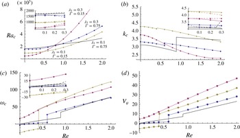
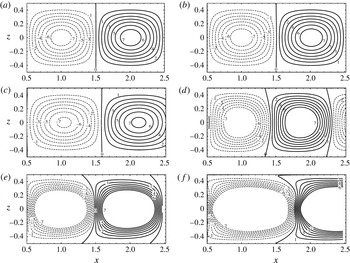
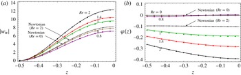
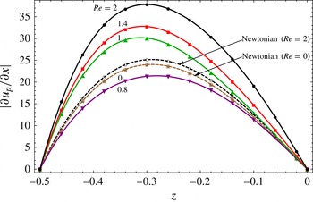
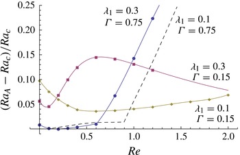
1. Introduction
The classical Rayleigh–Bénard–Poiseuille (RBP) problem consists of a fully-developed mixed convection bounded by horizontal rectangular walls, which results from the superposition of a horizontal pressure gradient and a vertical temperature gradient. Two types of instability can develop in RBP systems: (i) buoyancy-driven instabilities governed by the Rayleigh number
 $\mathit{Ra}$
, which give rise to structures in the form of thermoconvective rolls; and (ii) shear-flow instabilities governed by the Reynolds number
 $\mathit{Re}$
, which lead to Tollmien–Schlichting waves at high flow rates. In the present analysis, we will focus on buoyancy-driven instabilities and, hence, this study is restricted to low values of the Reynolds number in order to maintain all Tollmien–Schlichting modes stable.
In most cases, RBP systems are uniformly heated from below and subjected to a unidirectional throughflow with a laminar parabolic velocity profile due to the low Reynolds number imposed. In the conductive state, i.e. when the Rayleigh number is smaller than its first critical value, a Poiseuille flow is observed. When buoyancy forces are strong enough to overcome viscous forces, different types of thermoconvective structures can appear. We do not review here the numerous studies devoted to RBP flows of Newtonian fluids, but instead refer to the exhaustive bibliographical review presented by Nicolas (Reference Nicolas2002) and provide a summary of its major findings. Temporal linear stability analysis of such a flow in a duct of infinite lateral extent showed that the critical Rayleigh number is
 $\mathit{Ra}_{c}=1708$
for the appearance of longitudinal rolls (LRs), whose axes are parallel to the main flow direction. This critical value is Reynolds number independent and equal to the one found in the classical Rayleigh–Bénard (RB) problem. On the other hand, the throughflow stabilizes transverse rolls (TRs), whose axes are orthogonal to the main flow direction and to the temperature gradient direction. This linear analysis was also able to demonstrate that lateral confinement of the channel leads to stabilization of the flow and selects either TRs at small Reynolds numbers or LRs otherwise.
Contrary to the previously mentioned temporal analysis, in open systems (such as the RBP system), both the temporal and spatial growth of the disturbances must be considered and one must distinguish between the convective and the absolute nature of the instability (Briggs Reference Briggs1964). A methodology for doing so was applied to two-dimensional hydrodynamic instabilities by Huerre & Monkewitz (Reference Huerre and Monkewitz1985, Reference Huerre and Monkewitz1990). It was later extended to three-dimensional instabilities by Brevdo (Reference Brevdo1991). It consists of analysing the evolution and asymptotic behaviour of wave packets initially subjected to an impulse excitation. If its amplitude decays as it is advected downstream by the base flow, the system is convectively stable. Otherwise, the system is unstable. Two possibilities arise in the latter case. If the amplitude of an initially localized disturbance envelope eventually decays at any fixed location while it grows when observed in a coordinate system moving with its group speed, the system is convectively unstable. Otherwise, the system is absolutely unstable. Hence, all disturbances eventually leave a convectively unstable system in the absence of external forcing capable of providing a continuous perturbation source, allowing the system to return to its base state. On the other hand, certain disturbances initially present in an absolutely unstable system will eventually grow in time, forcing this system away from its original base state. In such cases, low-amplitude forcing plays a marginal role because the system becomes self-excited.
The transition from convective to absolute instability in RBP convection of Newtonian fluids has been studied by Muller, Lucke & Kamps (Reference Muller, Lucke and Kamps1992), Carrière & Monkewitz (Reference Carrière and Monkewitz1999) and Martinand, Carrière & Monkewitz (Reference Martinand, Carrière and Monkewitz2006) in the case of a pure fluid. These studies have been extended by Delache, Ouarzazi & Combarnous (Reference Delache, Ouarzazi and Combarnous2007), Delache & Ouarzazi (Reference Delache and Ouarzazi2008) and Ouarzazi et al. (Reference Ouarzazi, Mejni, Delache and Labrosse2008) to include the presence of a solid but porous matrix. In both systems, for a channel of infinite lateral extent, it has been shown that LRs are always convectively unstable whereas TRs can experience a transition to absolute instability. Comparisons with numerical and experimental studies validate these findings. Carrière & Monkewitz (Reference Carrière and Monkewitz1999) found that their marginal absolute instability curve for TRs predicts very accurately the instability transition observed in the two-dimensional numerical simulations performed by Nicolas, Mojtabi & Platten (Reference Nicolas, Mojtabi and Platten1997). Moreover, recent laboratory experiments conducted by Grandjean & Monkewitz (Reference Grandjean and Monkewitz2009) using water and mineral oil as working fluids proved that TRs indeed experience a transition to absolute instability as predicted by linear stability. Delache et al. (Reference Delache, Ouarzazi and Combarnous2007) reached the same conclusion when comparing their theoretical predictions with experimental data reported by Combarnous & Bories (Reference Combarnous and Bories1975).
Even though buoyancy-driven instabilities in Newtonian fluids have been extensively studied, the same cannot be said about their non-Newtonian counterparts. This is probably due to the fact that there is often a highly non-trivial coupling between the thermal–hydrodynamic problem and the rheological constitutive equation of the fluid. Recently, both theoreticians (Coelho, Pinho & Oliveira Reference Coelho, Pinho and Oliveira2002; Sheela-Francisca et al. Reference Sheela-Francisca, Tso, Hung and Rilling2012; Mokarizadeh, Asgharian & Raisi Reference Mokarizadeh, Asgharian and Raisi2013) and experimentalists (Nouar, Benaouda-Zouaoui & Desaubry Reference Nouar, Benaouda-Zouaoui and Desaubry2000; Peixinho, Desaubry & Lebouché Reference Peixinho, Desaubry and Lebouché2008) have been showing an increasing interest in mixed convection of non-Newtonian fluids. The reason for this is that such fluids can be found in a great number of applications, such as those in the food, cosmetics, pharmaceutical and petroleum industries, among others. More specifically, mixed convection of viscoelastic fluids through pipes and channels are relevant in polymer processing, where the melt flows at high temperatures before the extrusion process. In order to avoid the appearance of non-homogeneities in the final product, it is necessary to control the instabilities in the melt flow. Therefore, knowledge of the convective behaviour of the flow is an essential requirement in the design of polymer processing equipment.
For viscoelastic fluids, most of the existing studies focus either on hydrodynamic instabilities under isothermal conditions (Zhang et al.
Reference Zhang, Lashgari, Zaki and Brandt2013, and references therein), or on natural (RB) convection (see e.g. Green Reference Green1968; Vest & Arpaci Reference Vest and Arpaci1969; Sokolov & Tanner Reference Sokolov and Tanner1972; Eltayeb Reference Eltayeb1977; Rosenblat Reference Rosenblat1986; Martinez-Mardones & Perez-Garcia Reference Martinez-Mardones and Perez-Garcia1990; Larson Reference Larson1992; Martinez-Mardones & Perez-Garcia Reference Martinez-Mardones and Perez-Garcia1992; Martinez-Mardones et al.
Reference Martinez-Mardones, Tiemann, Walgraef and Zeller1996; Park & Lee Reference Park and Lee1996; Kolodner Reference Kolodner1998; Li & Khayat Reference Li and Khayat2005). In the latter case, linear stability analysis reveals that the onset of RB convection of viscoelastic fluids can be oscillatory instead of stationary, depending on the fluid elasticity. This behaviour was confirmed by the experimental results of Kolodner (Reference Kolodner1998) using DNA suspensions. Such a viscoelastic instability is usually observed in dilute polymer solutions, consisting of a Newtonian solvent and a polymeric solute. These solutions can be highly elastic while maintaining an essentially constant viscosity. They are, therefore, well represented by the Oldroyd-B constitutive model (Bird, Armstrong & Hassager Reference Bird, Armstrong and Hassager1987). As argued by Li & Khayat (Reference Li and Khayat2005), two regimes can be distinguished in the RB convection of an Oldroyd-B fluid: the weakly and strongly elastic fluid regimes. In the absence of throughflow, weakly (strongly) elastic fluids are identified as fluids with elasticity number smaller (larger) than
 ${\it\lambda}_{1}^{f}$
, where
 ${\it\lambda}_{1}^{f}$
is the critical elasticity number for the onset of oscillatory convection. It is important to emphasize that linear stability of RB convection in viscoelastic fluids was verified through a temporal analysis in the related aforementioned studies.
To the best of our knowledge, RBP convection of a viscoelastic fluid has not been considered before in the literature. Therefore, the major goal of the current work is to investigate the influence of elasticity effects on the physical mechanisms driving linear spatio-temporal instabilities in this flow of great technological importance. Our focus lies on a three-dimensional temporal linear stability analysis to determine the onset of convective instability. A two-dimensional spatial linear stability analysis is also utilized to distinguish it from the onset of absolute instability for TRs. A comprehensive study that includes the onset of absolute instability for LRs and oblique rolls (ORs) as well is beyond the scope of the present paper, but is the subject of current research in our group. Such an analysis has been presented by Brevdo (Reference Brevdo2009) and Diaz & Brevdo (Reference Diaz and Brevdo2011) for the mixed convection of a Newtonian fluid in porous media. However, it was made possible by the relatively simple algebraic nature of the dispersion relation in their problem. Whenever this is not the case, such as the differential dispersion relation derived in the present paper, the search for a zero group velocity vector subject to a simultaneous pinching condition in two complex wavenumber maps becomes a tremendous task, still in need of an efficient computational procedure (Suslov Reference Suslov2006). This contribution may be viewed as an extension of the stability of purely conducting quiescent states, i.e. the RB convection of a viscoelastic fluid, to the RBP configuration as well as an extension of RBP problem of Newtonian fluids to viscoelastic fluids. From a phenomenological standpoint, there is a close analogy between the current problem and the RBP convection of a Newtonian binary mixture with Soret effects (Jung, Lücke & Büchel Reference Jung, Lücke and Büchel1996; Büchel & Lücke Reference Büchel and Lücke2000a ; Hu, Ben Hadid & Henry Reference Hu, Ben Hadid and Henry2007).
This paper is organized as follows. Governing equations for this problem, including the steady base state and the formulation of its linear stability, are presented in § 2. After a description of numerical and analytical methods in § 3, a short review of the linear stability results for the version of this problem without throughflow is presented in § 4. In § 5, the combined influence of viscoelastic and throughflow parameters on the linear instability characteristics at the onset of convection is discussed. Section 6 presents the regions of convective and absolute instability for TRs in the Reynolds–Rayleigh number plane for various combinations of rheological parameters. In the latter two sections, results are presented and discussed for both weakly and strongly elastic fluids. The main conclusions of the present study are summarized in § 7.
2. Problem formulation
2.1. Governing equations
Consider an incompressible Oldroyd-B fluid layer of depth
 $h$
in the vertical
 $z$
-direction, with
 $z^{\ast }=0$
at its centre. This layer has an infinite extent in the
 $x$
and
 $y$
directions. Upper and lower horizontal walls are kept at constant temperatures
 $T_{0}^{\ast }$
and
 $T_{1}^{\ast }$
(
 ${>}T_{0}^{\ast }$
), respectively, and a constant pressure gradient is imposed in the
 $x$
-direction. All physical properties are assumed constant and evaluated at
 $T_{0}^{\ast }$
. They are given by
 ${\it\nu}$
for kinematic viscosity,
 ${\it\mu}$
for dynamic viscosity,
 $K$
for thermal diffusivity,
 ${\it\rho}$
for density,
 ${\it\beta}$
for thermal expansion coefficient,
 $g$
for gravitational acceleration,
 $e_{z}$
for the unit vector in the upward direction and, finally,
 ${\it\lambda}_{1}^{\ast }$
and
 ${\it\lambda}_{2}^{\ast }$
for relaxation and retardation times of the viscoelastic fluid, respectively. Assuming the Oberbeck–Boussinesq approximation holds, the governing equations for this problem are
 $$\begin{eqnarray}\displaystyle & \boldsymbol{{\rm\nabla}}\boldsymbol{\cdot }\boldsymbol{u}^{\ast }=0, & \displaystyle\end{eqnarray}$$
 $$\begin{eqnarray}\displaystyle & \displaystyle {\it\rho}\left(\frac{\partial \boldsymbol{u}^{\ast }}{\partial t^{\ast }}+(\boldsymbol{u}^{\ast }\boldsymbol{\cdot }\boldsymbol{{\rm\nabla}})\boldsymbol{u}^{\ast }\right)=-\boldsymbol{{\rm\nabla}}P^{\ast }+\boldsymbol{{\rm\nabla}}\boldsymbol{\cdot }{\bf\tau}^{\ast }+{\it\rho}{\it\beta}(T^{\ast }-T_{0}^{\ast })g\boldsymbol{e}_{\boldsymbol{z}}, & \displaystyle\end{eqnarray}$$
 $$\begin{eqnarray}\displaystyle & \displaystyle \frac{\partial T^{\ast }}{\partial t^{\ast }}+(\boldsymbol{u}^{\ast }\boldsymbol{\cdot }\boldsymbol{{\rm\nabla}})T^{\ast }=K{\rm\nabla}^{2}T^{\ast }, & \displaystyle\end{eqnarray}$$
 $$\begin{eqnarray}\displaystyle & {\bf\tau}^{\ast }+{\it\lambda}_{1}^{\ast }({\bf\tau}^{\ast })^{{\rm\nabla}}={\it\mu}\left({\bf\gamma}^{\ast }+{\it\lambda}_{2}^{\ast }({\bf\gamma}^{\ast })^{{\rm\nabla}}\right)\!. & \displaystyle\end{eqnarray}$$
 $$\begin{eqnarray}({\bf\tau}^{\ast })^{{\rm\nabla}}=\frac{\partial {\bf\tau}^{\ast }}{\partial t^{\ast }}+(\boldsymbol{u}^{\ast }\boldsymbol{\cdot }\boldsymbol{{\rm\nabla}}){\bf\tau}^{\ast }-(\boldsymbol{{\rm\nabla}}\boldsymbol{u}^{\ast })^{\text{T}}\boldsymbol{\cdot }{\bf\tau}^{\ast }-{\bf\tau}^{\ast }\boldsymbol{\cdot }(\boldsymbol{{\rm\nabla}}\boldsymbol{u}^{\ast }),\end{eqnarray}$$
where
 $\boldsymbol{u}^{\ast },P^{\ast }$
and
 $T^{\ast }$
represent the velocity, hydrostatic pressure, and temperature fields, respectively,
 ${\bf\tau}^{\ast }$
is the stress tensor and
 ${\bf\gamma}^{\ast }$
is the strain rate tensor. The above equations are subject to the following horizontal wall boundary conditions:
 $$\begin{eqnarray}\boldsymbol{u}^{\ast }=0\quad \text{at }z^{\ast }=\pm \frac{h}{2},\end{eqnarray}$$
 $$\begin{eqnarray}T^{\ast }=\left\{\begin{array}{@{}ll@{}}T_{0}^{\ast }\quad & \text{at }z^{\ast }=+{\displaystyle \frac{h}{2}}\\ T_{1}^{\ast }\quad & \text{at }z^{\ast }=-{\displaystyle \frac{h}{2}}.\end{array}\right.\end{eqnarray}$$
2.2. Base state
System (2.1)–(2.5), subjected to boundary conditions (2.6) and (2.7), has a steady state that corresponds to a combination of plane Poiseuille flow with vertical thermal stratification. This base flow is written as
 $$\begin{eqnarray}\displaystyle & \displaystyle \boldsymbol{u}_{b}^{\ast }=U_{0}^{\ast }\left(1-4\frac{z^{\ast 2}}{h^{2}}\right)\boldsymbol{e}_{\boldsymbol{x}}, & \displaystyle\end{eqnarray}$$
 $$\begin{eqnarray}\displaystyle & \displaystyle T_{b}^{\ast }=T_{0}^{\ast }+(T_{1}^{\ast }-T_{0}^{\ast })\left(\frac{1}{2}-\frac{z^{\ast }}{h}\right), & \displaystyle\end{eqnarray}$$
 $$\begin{eqnarray}\displaystyle & \displaystyle P_{b}^{\ast }=P_{0}^{\ast }+\frac{{\it\rho}{\it\beta}gh(T_{1}^{\ast }-T_{0}^{\ast })}{2}\left(\frac{z^{\ast }}{h}-\frac{z^{\ast 2}}{h^{2}}\right)-\frac{8{\it\mu}U_{0}^{\ast }}{h}\left(\frac{x^{\ast }}{h}\right), & \displaystyle\end{eqnarray}$$
 $U_{0}^{\ast }$
being defined as the maximum steady-state throughflow velocity. This solution has an associated stress tensor given by
 $$\begin{eqnarray}{\bf\tau}_{b}^{\ast }(z^{\ast })=\left(\begin{array}{@{}ccc@{}}\displaystyle 128\frac{{\it\mu}({\it\lambda}_{1}^{\ast }-{\it\lambda}_{2}^{\ast })(U_{0}^{\ast })^{2}}{h^{2}}\frac{z^{\ast 2}}{h^{2}} & 0 & -8{\displaystyle \frac{U_{0}^{\ast }{\it\mu}}{h}}{\displaystyle \frac{z^{\ast }}{h}}\\ 0 & 0 & 0\\ \displaystyle -8\frac{U_{0}^{\ast }{\it\mu}}{h}\frac{z^{\ast }}{h} & 0 & 0\end{array}\right),\end{eqnarray}$$
where shear stress components
 $({\bf\tau}_{b}^{\ast })^{(1,3)}=({\bf\tau}_{b}^{\ast })^{(3,1)}=-8(U_{0}^{\ast }{\it\mu}/h^{2})z^{\ast }$
also appear for Newtonian fluids and vary linearly across the vertical channel section. For the Oldroyd-B model, this linear variation in the vertical direction of the shear stress components induces quadratic variations in the normal stress component
 $({\bf\tau}_{b}^{\ast })^{(1,1)}=128{\it\mu}({\it\lambda}_{1}^{\ast }-{\it\lambda}_{2}^{\ast })(U_{0}^{\ast 2}/h^{4})(z^{\ast })^{2}$
. This component vanishes for Newtonian fluids (i.e.
 ${\it\lambda}_{1}^{\ast }={\it\lambda}_{2}^{\ast }$
).
A separate scaling is now introduced for the base flow in order to write it in dimensionless form. This scaling is based on
 $h,U_{0}^{\ast },{\it\mu}U_{0}^{\ast }/h$
and
 ${\rm\Delta}T^{\ast }=T_{1}^{\ast }-T_{0}^{\ast }$
as reference quantities for length, velocity, stress components and temperature, respectively. The base flow solutions (2.8)–(2.11) can now be re-written in dimensionless form as
 $$\begin{eqnarray}\displaystyle & \boldsymbol{u}_{b}=(1-4z^{2})\boldsymbol{e}_{\boldsymbol{x}}=f(z)\boldsymbol{e}_{\boldsymbol{x}}, & \displaystyle\end{eqnarray}$$
 $$\begin{eqnarray}\displaystyle & \displaystyle T_{b}={\textstyle \frac{1}{2}}-z, & \displaystyle\end{eqnarray}$$
 $$\begin{eqnarray}\displaystyle & {\it\tau}_{b}^{(1,3)}=-8z, & \displaystyle\end{eqnarray}$$
 $$\begin{eqnarray}\displaystyle & \displaystyle {\it\tau}_{b}^{(1,1)}=128\mathit{De}\left(1-\frac{{\it\lambda}_{2}^{\ast }}{{\it\lambda}_{1}^{\ast }}\right)z^{2}, & \displaystyle\end{eqnarray}$$
 $\mathit{De}$
is the Deborah number defined as
 $\mathit{De}={\it\lambda}_{1}^{\ast }U_{0}^{\ast }/h$
. This parameter is a measure of fluid elasticity or, in other words, a measure of the fluid delayed reaction to its own advection. It is important to note that the dimensionless expressions for
 ${\it\tau}_{b}^{(1,3)}$
and
 ${\it\tau}_{b}^{(1,1)}$
above show that these two stress components are related according to the formula
 $$\begin{eqnarray}{\it\tau}_{b}^{(1,1)}=2\mathit{De}\left(1-\frac{{\it\lambda}_{2}^{\ast }}{{\it\lambda}_{1}^{\ast }}\right)({\it\tau}_{b}^{(1,3)})^{2}.\end{eqnarray}$$
2.3. Linear stability analysis
Once the base flow (2.8)–(2.11) has been defined, one can verify its asymptotic (
 $t\rightarrow \infty$
) stability by following the classical linear stability formalism. In order to do so, dependent variables in the governing equations (2.1)–(2.7) are replaced by this base flow superposed with infinitesimal perturbations. Since these perturbations are considered small, one can linearize the resulting equations to deduce the perturbation governing equations. It should be noted that the pressure field is eliminated here by taking the double curl of the momentum perturbation equation. These equations are written in dimensionless form by introducing a new scaling based on
 $h,h^{2}/K,K/h,{\it\mu}K/h^{2}$
and
 ${\rm\Delta}T^{\ast }=T_{1}^{\ast }-T_{0}^{\ast }$
as reference quantities for length, time, perturbation velocity, stress components and temperature, respectively. They can be combined in such a way as to reduce this system to only two equations: one for the vertical component of the perturbation velocity
 $w_{p}$
and the other for the temperature perturbation
 ${\it\theta}_{p}$
,
 $$\begin{eqnarray}\displaystyle & & \displaystyle \frac{1}{\mathit{Pr}}\left(\frac{\partial }{\partial t}{\rm\nabla}^{2}w_{p}\right)+\mathit{Re}\left(\,f(z){\rm\nabla}^{2}-f^{\prime \prime }(z)\right)\frac{\partial w_{p}}{\partial x}-\mathit{Ra}{\rm\nabla}_{\bot }^{2}{\it\theta}_{p}\nonumber\\ \displaystyle & & \displaystyle \quad +\,\frac{\partial }{\partial z}\left(\frac{\partial ^{2}{\it\tau}_{p}^{(1,1)}}{\partial x^{2}}+\frac{\partial ^{2}{\it\tau}_{p}^{(2,2)}}{\partial y^{2}}+2\frac{\partial ^{2}{\it\tau}_{p}^{(1,2)}}{\partial x\partial y}\right)\nonumber\\ \displaystyle & & \displaystyle \quad +\left(\frac{\partial ^{2}}{\partial z^{2}}-\frac{\partial ^{2}}{\partial x^{2}}-\frac{\partial ^{2}}{\partial y^{2}}\right)\left(\frac{\partial {\it\tau}_{p}^{(1,3)}}{\partial x}+\frac{\partial {\it\tau}_{p}^{(2,3)}}{\partial y}\right)-\frac{\partial }{\partial z}{\rm\nabla}_{\bot }^{2}{\it\tau}_{p}^{(3,3)}=0,\end{eqnarray}$$
 $$\begin{eqnarray}\displaystyle & & \displaystyle \left(\frac{\partial }{\partial t}-{\rm\nabla}^{2}+\mathit{Re}\,\mathit{Pr}\,f(z)\frac{\partial }{\partial x}\right){\it\theta}_{p}-w_{p}=0,\end{eqnarray}$$
 $$\begin{eqnarray}{\rm\nabla}^{2}=\frac{\partial ^{2}}{\partial x^{2}}+\frac{\partial ^{2}}{\partial y^{2}}+\frac{\partial ^{2}}{\partial z^{2}}\quad \text{and}\quad {\rm\nabla}_{\bot }^{2}=\frac{\partial ^{2}}{\partial x^{2}}+\frac{\partial ^{2}}{\partial y^{2}},\end{eqnarray}$$
which are subject to dimensionless boundary conditions at the upper and lower walls,
 $$\begin{eqnarray}\displaystyle & \displaystyle w_{p}=\frac{\partial w_{p}}{\partial z}=0\quad \text{at }z=\pm 1/2, & \displaystyle\end{eqnarray}$$
 $$\begin{eqnarray}\displaystyle & {\it\theta}_{p}=0\quad \text{at }z=\pm 1/2. & \displaystyle\end{eqnarray}$$
Dimensionless governing equations for the perturbation stress components
 ${\it\tau}_{p}^{(i,j)}$
have been obtained from constitutive relation (2.4), linearized around the base state. These components depend on the other perturbations, and their functional dependence is given in modal form in appendix B for the two-dimensional case. Nevertheless, it is important to remark that the nonlinear character of constitutive relation (2.4) introduces velocity and stress tensor components associated with the base state into these governing equations. Such a feature increases considerably the model complexity and, hence, its numerical simulation, compared to its two limiting cases: the RB convection of Oldroyd-B fluids (
 $\mathit{Re}=0$
) and the RBP convection of Newtonian fluids (
 ${\it\Gamma}=1$
).
The dimensionless parameters appearing in the governing equations (2.17) and (2.18) are the Rayleigh number
 $\mathit{Ra}$
, Reynolds number
 $\mathit{Re}$
, Prandtl number
 $\mathit{Pr}$
, dimensionless relaxation time or elasticity number
 ${\it\lambda}_{1}$
and dimensionless retardation time
 ${\it\lambda}_{2}$
. These numbers are respectively defined as
 $$\begin{eqnarray}\displaystyle & \displaystyle \mathit{Ra}=\frac{g{\it\beta}{\rm\Delta}T^{\ast }h^{3}}{{\it\nu}K}, & \displaystyle\end{eqnarray}$$
 $$\begin{eqnarray}\displaystyle & \displaystyle \mathit{Re}=\frac{U_{0}^{\ast }h}{{\it\nu}}, & \displaystyle\end{eqnarray}$$
 $$\begin{eqnarray}\displaystyle & \displaystyle \mathit{Pr}=\frac{{\it\nu}}{K}, & \displaystyle\end{eqnarray}$$
 $$\begin{eqnarray}\displaystyle & \displaystyle {\it\lambda}_{1}=\frac{{\it\lambda}_{1}^{\ast }}{h^{2}/K}, & \displaystyle\end{eqnarray}$$
 $$\begin{eqnarray}\displaystyle & \displaystyle {\it\lambda}_{2}=\frac{{\it\lambda}_{2}^{\ast }}{h^{2}/K}, & \displaystyle\end{eqnarray}$$
 $$\begin{eqnarray}{\it\Gamma}=\frac{{\it\lambda}_{2}^{\ast }}{{\it\lambda}_{1}^{\ast }},\end{eqnarray}$$
is used in this study instead of
 ${\it\lambda}_{2}$
. Typical fluids satisfying constitutive relation (2.4) are solutions composed of a Newtonian solvent and a polymeric solute with viscosities
 ${\it\mu}_{s}$
and
 ${\it\mu}_{p}$
, respectively. The viscosity of the solution is given by
 ${\it\mu}={\it\mu}_{s}+{\it\mu}_{p}$
and, hence, the ratio between retardation and relaxation times is
 ${\it\Gamma}={\it\mu}_{s}/{\it\mu}$
(Bird et al.
Reference Bird, Armstrong and Hassager1987). Furthermore,
 ${\it\lambda}_{1}$
is employed instead of
 $\mathit{De}$
as a measure of fluid elasticity in almost all available literature on thermal convection of viscoelastic fluids (Green Reference Green1968; Vest & Arpaci Reference Vest and Arpaci1969; Sokolov & Tanner Reference Sokolov and Tanner1972; Eltayeb Reference Eltayeb1977; Rosenblat Reference Rosenblat1986; Martinez-Mardones & Perez-Garcia Reference Martinez-Mardones and Perez-Garcia1990; Larson Reference Larson1992; Martinez-Mardones & Perez-Garcia Reference Martinez-Mardones and Perez-Garcia1992; Martinez-Mardones et al.
Reference Martinez-Mardones, Tiemann, Walgraef and Zeller1996; Park & Lee Reference Park and Lee1996; Kolodner Reference Kolodner1998; Li & Khayat Reference Li and Khayat2005). However, the former is now a measure of the fluid delayed reaction to its own thermal diffusion, instead of advection, because of the dimensionless form chosen in definition (2.25). This is an appropriate choice for the present study since it is restricted to low Reynolds numbers. Therefore,
 $\mathit{De}$
is replaced by
 ${\it\lambda}_{1}$
in relation (2.15) using
 $\mathit{De}={\it\lambda}_{1}\mathit{Re}\mathit{Pr}$
. Finally, it should be noted that
 ${\it\lambda}_{1}\geqslant {\it\lambda}_{2}$
, i.e.
 ${\it\Gamma}\in [0,1]$
and that the Maxwellian model is recovered when
 ${\it\Gamma}=0$
(or
 ${\it\lambda}_{2}=0$
) whereas the Newtonian model is recovered when
 ${\it\Gamma}=1$
(or
 ${\it\lambda}_{1}={\it\lambda}_{2}$
).
We seek three-dimensional normal modes in the form
 $$\begin{eqnarray}\left\{w_{p},{\it\theta}_{p},{\it\tau}_{p}^{(i,j)}\right\}(x,y,z,t)=\left\{w_{n},{\it\theta}_{n},{\it\tau}_{n}^{(i,j)}\right\}(z)\exp (\text{i}(k_{x}x+k_{y}y-{\it\omega}t)),\end{eqnarray}$$
where
 $k_{x}$
and
 $k_{y}$
are the wavenumbers in the
 $x$
- and
 $y$
-directions, respectively, and
 ${\it\omega}$
is the frequency. All three parameters are complex numbers, since both temporal and spatial stability analyses were performed in the present study. Upon substitution of functional form (2.28) into (2.17) and (2.18), as well as the associated perturbation stress component equations, it is possible to reduce the resulting system to two coupled ordinary differential equations (ODEs) for the linear perturbation normal mode amplitudes
 $w_{n}(z)$
and
 ${\it\theta}_{n}(z)$
. They are given by
 $$\begin{eqnarray}\displaystyle & & \displaystyle \frac{\text{i}}{\mathit{Pr}}((k_{x}\mathit{Re}\,\mathit{Pr}\,f(z)-{\it\omega})\left(\text{D}^{2}-k^{2}\right)-k_{x}\mathit{Re}\,\mathit{Pr}\,f^{\prime \prime }(z))w_{n}(z)+k^{2}\text{D}{\it\tau}_{n}^{(3,3)}(z)\nonumber\\ \displaystyle & & \displaystyle \quad +\,\text{D}\text{L}(w_{n}(z))+\left(\text{D}^{2}+k^{2}\right)\text{J}(w_{n}(z))+\mathit{Ra}k^{2}{\it\theta}_{n}(z)=0,\end{eqnarray}$$
 $$\begin{eqnarray}w_{n}(z)+\left(\text{D}^{2}-k^{2}-\text{i}k_{x}\mathit{Re}\,\mathit{Pr}\,f(z)+\text{i}{\it\omega}\right){\it\theta}_{n}(z)=0\end{eqnarray}$$
where
 $k^{2}=k_{x}^{2}+k_{y}^{2}$
,
 $\text{D}=\text{d}/\text{d}z$
, and the dependence of operators
 $\text{L}$
and
 $\text{J}$
, as well as stress component
 ${\it\tau}^{(3,3)}(z)$
, on
 $w_{n}(z)$
is given by the expressions
 $$\begin{eqnarray}\displaystyle \text{L}(w_{n}(z)) & = & \displaystyle -k_{x}^{2}{\it\tau}_{n}^{(1,1)}(z)-k_{y}^{2}{\it\tau}_{n}^{(2,2)}(z)-2k_{x}k_{y}{\it\tau}_{n}^{(1,2)}(z)\nonumber\\ \displaystyle & = & \displaystyle \left[2\text{i}k_{x}\mathit{Re}\,\mathit{Pr}\,{\it\lambda}_{1}f^{\prime }(z)\text{J}(w_{n}(z))+ (\!2\text{i}k_{x}\mathit{Re}\,\mathit{Pr}\,{\it\lambda}_{1}(2{\it\Gamma}-1)f^{\prime }(z)\text{D}^{2}\right.\nonumber\\ \displaystyle & & \displaystyle +\,4k_{x}^{2}\mathit{Re}^{2}\mathit{Pr}^{2}{\it\lambda}_{1}^{2}(1-{\it\Gamma})(f^{\prime }(z))^{2}+2k^{2}+2\text{i}k^{2}k_{x}\mathit{Re}\,\mathit{Pr}\,{\it\lambda}_{1}{\it\Gamma}f(z)\nonumber\\ \displaystyle & & \displaystyle -\,2\text{i}k^{2}{\it\omega}{\it\lambda}_{1}{\it\Gamma}\text{D}+4k_{x}^{2}\mathit{Re}^{2}\mathit{Pr}^{2}{\it\lambda}_{1}^{2}(1-{\it\Gamma})f^{\prime }(z)f^{\prime \prime }(z)\nonumber\\ \displaystyle & & \displaystyle +\left.2\text{i}k^{2}k_{x}\mathit{Re}\,\mathit{Pr}\,{\it\lambda}_{1}{\it\Gamma}f^{\prime }(z)\!)w_{n}(z)\right]/[1+\text{i}k_{x}\mathit{Re}\,\mathit{Pr}\,{\it\lambda}_{1}f(z)-\text{i}{\it\omega}{\it\lambda}_{1}],\end{eqnarray}$$
 $$\begin{eqnarray}\displaystyle \text{J}(w_{n}(z)) & = & \displaystyle \text{i}k_{x}{\it\tau}_{n}^{(1,3)}(z)+\text{i}k_{y}{\it\tau}_{n}^{(2,3)}(z)\nonumber\\ \displaystyle & = & \displaystyle \left[\text{i}k_{x}\mathit{Re}\,\mathit{Pr}\,{\it\lambda}_{1}f^{\prime }(z){\it\tau}_{n}^{(3,3)}(z)- (\!2\text{i}k_{x}\mathit{Re}\,\mathit{Pr}\,{\it\lambda}_{1}{\it\Gamma}f^{\prime }(z)\text{D}-\text{i}{\it\omega}{\it\lambda}_{1}{\it\Gamma}\text{D}^{2}\right.\nonumber\\ \displaystyle & & \displaystyle +\,(1+k^{2})(1+\text{i}k_{x}\mathit{Re}\,\mathit{Pr}\,{\it\lambda}_{1}{\it\Gamma}f(z))+\text{i}k_{x}\mathit{Re}\,\mathit{Pr}\,{\it\lambda}_{1}(1-{\it\Gamma})f^{\prime \prime }(z)-\text{i}{\it\omega}k^{2}{\it\lambda}_{1}{\it\Gamma}\nonumber\\ \displaystyle & & \displaystyle +\left.2k_{x}^{2}\mathit{Re}^{2}\mathit{Pr}^{2}{\it\lambda}_{1}^{2}(1-{\it\Gamma})(f^{\prime }(z))^{2}\! )w_{n}(z)\right]/[1+\text{i}k_{x}\mathit{Re}\,\mathit{Pr}\,{\it\lambda}_{1}f(z)-\text{i}{\it\omega}{\it\lambda}_{1}],\end{eqnarray}$$
 $$\begin{eqnarray}\displaystyle {\it\tau}_{n}^{(3,3)}(z) & = & \displaystyle \left[((2+2\text{i}k_{x}\mathit{Re}\,\mathit{Pr}\,{\it\lambda}_{1}{\it\Gamma}f(z)-2\text{i}{\it\omega}{\it\lambda}_{1}{\it\Gamma})\text{D}\right.\nonumber\\ \displaystyle & & \displaystyle +\left.2\text{i}k_{x}\mathit{Re}\,\mathit{Pr}\,{\it\lambda}_{1}(1-{\it\Gamma})f^{\prime }(z)\!)/(1+\text{i}k_{x}\mathit{Re}\,\mathit{Pr}\,{\it\lambda}_{1}f(z)-\text{i}{\it\omega}{\it\lambda}_{1})\right]w_{n}(z),\end{eqnarray}$$
 $$\begin{eqnarray}\displaystyle & w_{n}=\text{D}w_{n}=0\quad \text{at }z=\pm 1/2, & \displaystyle\end{eqnarray}$$
 $$\begin{eqnarray}\displaystyle & {\it\theta}_{n}=0\quad \text{at }z=\pm 1/2, & \displaystyle\end{eqnarray}$$
3. Solution methodology
3.1. Galerkin method
Approximate solutions for system (2.29)–(2.35) can be generated using the standard Galerkin method, where the vertical velocity and temperature normal mode perturbation amplitudes are expanded as
 $$\begin{eqnarray}w_{n}(z)=\mathop{\sum }_{i=0}^{N}{\it\psi}_{i}(z)\bar{w}_{i}\quad \text{with }{\it\psi}_{i}(z)=(1-4z^{2})^{2}z^{i}\end{eqnarray}$$
and
 $$\begin{eqnarray}{\it\theta}_{n}(z)=\mathop{\sum }_{i=0}^{N}{\it\phi}_{i}(z)\bar{{\it\theta}}_{i}\quad \text{with }{\it\phi}_{i}(z)=(1-4z^{2})z^{i},\end{eqnarray}$$
respectively. In these expansions,
 ${\it\psi}_{i}(z)$
and
 ${\it\phi}_{i}(z)$
are the eigenfunctions whereas
 $\bar{w}_{i}$
and
 $\bar{{\it\theta}}_{i}$
are the amplitude coefficients. Multiplying (2.29) by
 ${\it\psi}_{i}(z)$
as well as (2.30) by
 ${\it\phi}_{i}(z)$
, and integrating both results over the domain length, leads to
 $$\begin{eqnarray}\mathop{\sum }_{j=0}^{N}\mathscr{A}_{i,j}\bar{w}_{j}+\mathop{\sum }_{j=0}^{N}\mathscr{B}_{i,j}\bar{{\it\theta}}_{j}=0\quad \text{and}\quad \bar{w}_{i}+\mathop{\sum }_{j=0}^{N}\mathscr{C}_{i,j}\bar{{\it\theta}}_{j}=0,\end{eqnarray}$$
which can be combined into the single equation
 $$\begin{eqnarray}\mathop{\sum }_{j=0}^{N}\mathscr{D}_{i,j}\bar{{\it\theta}}_{j}=0\quad \text{with }\mathscr{D}=\mathscr{B}-\mathscr{A}\,\mathscr{C},\end{eqnarray}$$
which yields non-trivial solutions only when
 $$\begin{eqnarray}\mathfrak{D}=\det [\mathscr{D}]=0\end{eqnarray}$$
is satisfied, which is the resulting algebraic dispersion relation.
In the present work, an initial analysis is performed using the approximate version of the algebraic dispersion relation obtained by setting
 $N=0$
, i.e. using a single-term truncation. Such an approximation was employed by Kolka & Ierley (Reference Kolka and Ierley1987) to investigate the linear onset of RB convection with Oldroyd-B fluids. That problem is similar to the present one, but without throughflow. They also generated accurate numerical solutions using a spectral Chebyshev
 ${\it\tau}$
-method and noted that the single-term Galerkin solutions were accurate to within 5 %, but only when the boundary conditions used in the present work are considered.
Carrière & Monkewitz (Reference Carrière and Monkewitz1999) also employed a single-term truncation in their work. When studying the RB convection of Newtonian fluids, they found a critical Rayleigh number of 1749.98, which is only 2.5 % higher than the exact value. Moreover, these authors also considered the influence of throughflow in their work, which was included in their single-term approximation as well. The behaviour extracted from this analytical formula is in excellent agreement with the small-Reynolds-number expansion obtained by Muller et al. (Reference Muller, Lucke and Kamps1992).
These two studies motivated us to examine the single-term Galerkin expansion, or single-term truncation, for the present problem. It allows the generation of analytical expressions that can guide a more computationally intensive numerical analysis as well as future laboratory experiments, owing to its simplicity. Even when their error in quantitative predictions was high, their qualitative behaviour prediction was accurate enough to guide additional numerical efforts. Setting
 $N=0$
and performing some symbolic manipulations, such an algebraic dispersion relation is obtained. It is provided in appendix A, owing due to its very long coefficients. However, in the limit of small values of the Deborah number (
 $\mathit{De}={\it\lambda}_{1}\mathit{Re}\mathit{Pr}$
), this dispersion relation can be written as
 $$\begin{eqnarray}\mathfrak{D}=G(F_{1}+k_{x}\mathit{Re}\,F_{2})-{\textstyle \frac{27}{4}}k^{2}\mathit{Ra}(1-\text{i}{\it\omega}{\it\lambda}_{1})^{2}=0,\end{eqnarray}$$
where the additional parameters are defined as
 $$\begin{eqnarray}\displaystyle & \displaystyle G=6k_{x}\mathit{Re}\,\mathit{Pr}-7({\it\omega}+\text{i}\,f_{1}), & \displaystyle\end{eqnarray}$$
 $$\begin{eqnarray}\displaystyle & \displaystyle F_{1}=(1-\text{i}{\it\omega}{\it\lambda}_{1})^{2}\frac{{\it\omega}}{\mathit{Pr}}\,f_{2}+\text{i}(1-\text{i}{\it\omega}{\it\lambda}_{1})(1-\text{i}{\it\omega}{\it\lambda}_{1}{\it\Gamma})\,f_{4}, & \displaystyle\end{eqnarray}$$
 $$\begin{eqnarray}\displaystyle & \displaystyle F_{2}=-{\textstyle \frac{2}{11}}(1-\text{i}{\it\omega}{\it\lambda}_{1})^{2}\,f_{3}+{\it\lambda}_{1}(1-{\it\Gamma})\mathit{Pr}\,f_{5}, & \displaystyle\end{eqnarray}$$
 $$\begin{eqnarray}f_{1}=k^{2}+10,\quad f_{2}=k^{2}+12,\quad f_{3}=5k^{2}+22,\end{eqnarray}$$
 $$\begin{eqnarray}f_{4}=f_{2}^{2}+360\quad \text{and}\quad f_{5}={\textstyle \frac{10}{11}}k^{4}+24k^{2}+432.\end{eqnarray}$$
It is important to note that expression (3.6) reduces to the dispersion relation derived by Kolka & Ierley (Reference Kolka and Ierley1987) for the RB convection of Oldroyd-B fluids when
 $\mathit{Re}=0$
and
 ${\it\Gamma}\neq 1$
, as well as the dispersion relation derived by Carrière & Monkewitz (Reference Carrière and Monkewitz1999) for the RBP convection of Newtonian fluids when
 ${\it\Gamma}=1$
and
 $\mathit{Re}\neq 0$
.
As shown in the following sections, the single-term Galerkin truncation does not present accurate results over the entire range of parameters under consideration, and higher-order truncation becomes necessary. However, the Galerkin expansion requires the calculation of several integral coefficients inside matrices
 $\mathscr{A}$
,
 $\mathscr{B}$
and
 $\mathscr{C}$
. This is a difficult task because the complexity of the governing equations makes the evaluation of (3.5) a higher computational time consuming task, especially when increasing the number of terms
 $N$
. Therefore, a shooting method is preferred in order to generate the numerical results. Converged Galerkin method results with up to
 $N=20$
terms are used only to verify the accuracy of the shooting method, which is explained next.
3.2. Shooting method
The solution obtained from the truncated Galerkin method derived in the previous section provides the initial estimates for the root-searching algorithm developed to find their respective accurate solutions for all existing modes. A similar algorithm was employed in previous studies to analyse the linear instability of spatially developing mixing layers in transverse jets (de B. Alves, Kelly & Karagozian Reference de B. Alves, Kelly and Karagozian2008; Kelly & Alves Reference Kelly and de B. Alves2008). It is a shooting method based on built-in functions from the software Mathematica (Wolfram Reference Wolfram2003).
System (2.29)–(2.33) is first changed from a boundary value problem into an initial value one by re-writing boundary conditions (2.34) and (2.35) as
 $$\begin{eqnarray}w_{n}=\text{D}w_{n}=0,\quad \text{D}^{2}w_{n}=\mathfrak{C}_{1},\quad \text{D}^{3}w_{n}=\mathfrak{C}_{2}\quad \text{at }z=-1/2,\end{eqnarray}$$
 $$\begin{eqnarray}{\it\theta}_{n}=0\quad \text{and}\quad \text{D}{\it\theta}_{n}=\mathfrak{C}_{3}\quad \text{at }z=-1/2,\end{eqnarray}$$
respectively. Additional constants
 $\mathfrak{C}_{1}$
,
 $\mathfrak{C}_{2}$
and
 $\mathfrak{C}_{3}$
must then be chosen in such a way as to guarantee that solutions
 $w_{n}$
and
 ${\it\theta}_{n}$
satisfy the three boundary conditions at
 $z=+(1/2)$
from (2.34) and (2.35) left behind when writing their initial condition counterparts in (3.12) and (3.13). Since this is an eigenvalue problem, one of these constants must remain undetermined. In the present work, the entire problem is re-scaled by
 $\mathfrak{C}_{3}$
. Such a scaling is equivalent to setting
 $\mathfrak{C}_{3}=1$
, which is done to avoid having to redefine our dependent variables. Two unknown real parameters, called here
 $\mathscr{P}_{1}$
and
 $\mathscr{P}_{2}$
, can now be determined in conjunction with
 $\mathfrak{C}_{1}$
and
 $\mathfrak{C}_{2}$
by solving this modified system because
 $\mathfrak{C}_{3}$
is a complex number in general. The choice of parameters
 $\mathscr{P}_{1}$
and
 $\mathscr{P}_{2}$
to be determined, however, depends on the problem at hand.
Before presenting the shooting method results, the two numerical procedures employed are briefly described. The first one uses built-in function NDSolve to march ODEs (2.29) and (2.30) from
 $z=-(1/2)$
to
 $+(1/2)$
using initial conditions (2.34) and (2.35), with given estimates for
 $\mathscr{P}_{1},\mathscr{P}_{2},\text{Re}[\mathfrak{C}_{1}],\text{Im}[\mathfrak{C}_{1}]$
,
 $\text{Re}[\mathfrak{C}_{2}]$
and
 $\text{Im}[\mathfrak{C}_{2}]$
as well as fixed values for the remaining parameters. It switches between Adams, backwards-differencing-formula (BDF) and Runge–Kutta schemes depending on local problem stiffness. Furthermore, explicit and implicit versions of these schemes are selected based on the local step size, which is adjusted automatically according to the prescribed absolute and relative errors. They are imposed a priori by fixing the number of digits to be used in the computations. In the current study, this number was set to 16, 18 and 20 in order to verify solution convergence. Such a procedure is programed into function
 $\mathfrak{F}_{1}$
, which yields a real vector whose six elements are the values of
 $\text{Re}[w_{n}],\text{Im}[w_{n}],\text{Re}[\text{D}w_{n}],\text{Im}[\text{D}w_{n}],\text{Re}[{\it\theta}_{n}]$
and
 $\text{Im}[{\it\theta}_{n}]$
evaluated at
 $z=+(1/2)$
. Now the second procedure can be employed. It uses built-in function FindRoot to search for estimates that satisfy
 $\mathfrak{F}_{1}\simeq 0$
according to the absolute and relative tolerances prescribed. Brent’s method is used with this function in the present work, requiring two initial guesses for each estimate. The search for unstable modes is intrinsically related to the search for adequate initial guesses. Hence, this process also depends on the nature of the instability mechanism, which is discussed in more detail in the following two subsections.
3.3. Temporal stability analysis
The onset of convection in spatially developing flows may be induced by convective and/or absolute instability mechanisms. In order to determine the onset of convective instability, a temporal stability analysis is employed first. It considers only spatially sinusoidal disturbances, i.e. normal modes with real wavenumbers
 $k_{x}$
and
 $k_{y}$
and a complex frequency
 ${\it\omega}={\it\omega}_{r}+\text{i}{\it\omega}_{i}$
. The neutral stability boundary separating stable and unstable regions is defined by
 ${\it\omega}_{i}=0$
, where the critical Rayleigh number
 $\mathit{Ra}_{c}$
is found at its minimum. This onset will be induced by a stationary mode of instability when
 ${\it\omega}_{r}=0$
, otherwise it will be induced by an oscillatory mode of instability when
 ${\it\omega}_{r}\neq 0$
. Hence, in accordance with the definitions introduced in the previous subsection, the additional parameters to be determined in this analysis are
 $\mathscr{P}_{1}={\it\omega}_{r}$
and
 $\mathscr{P}_{2}=\mathit{Ra}$
.
We first focus our attention on the convective instability of LRs, whose wave vector is perpendicular to the throughflow, i.e.
 $k_{x}=0$
. Since
 $\mathit{Re}$
only appears multiplied by
 $k_{x}$
in the system (2.29)–(2.33), stability results for LRs are the same as those obtained in the absence of throughflow, i.e.
 $\mathit{Re}=0$
. Both stationary and oscillatory instabilities can develop depending on the choice of
 ${\it\lambda}_{1}$
and
 ${\it\Gamma}$
. A literature review of this particular case is presented in § 4.
The Squire theorem, which states that two-dimensional disturbances are more unstable than three-dimensional ones, is not valid in this problem. For TRs and ORs, which represent general three-dimensional disturbances, wavenumber
 $k_{y}$
enters the problem through the modified wavenumber
 $k$
, defined earlier as
 $k^{2}=k_{x}^{2}+k_{y}^{2}$
. Hence, one can operate on system (2.29)–(2.33) with the following Squire transformation:
 $$\begin{eqnarray}k_{x}\mathit{Re}_{3D}=k\mathit{Re},\end{eqnarray}$$
before solving it. This transformation reduces the general three-dimensional problem to an equivalent two-dimensional counterpart of TRs, since the wave vector of TRs is parallel to the throughflow, i.e.
 $k_{y}=0$
.
In order to determine the values of
 $\mathscr{P}_{1}={\it\omega}_{r}$
and
 $\mathscr{P}_{2}=\mathit{Ra}$
for the most unstable temporal modes, estimates are first generated using (3.6). This is achieved by identifying the lines where real and imaginary parts of this equation are zero with respect to
 ${\it\omega}_{r}$
and
 $\mathit{Ra}$
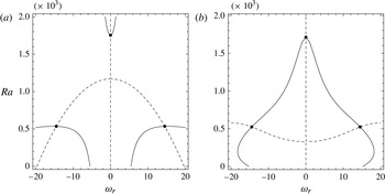
. Hence, unstable modes appear as the points where the two lines intersect. Figure 1(a) shows this behaviour for
 $\mathit{Re}=0,\mathit{Pr}=10,{\it\lambda}_{1}=0.3$
and
 ${\it\Gamma}=0.15$
obtained at
 $k=3$
, confirming the presence of three modes at this wavenumber. They are located at
 $({\it\omega}_{r},\mathit{Ra})\simeq (-14.527,534.96)$
,
 $(0,1753.6)$
and
 $(+14.527,534.96)$
.
Temporally unstable modes (solid points) for
 $\mathit{Re}=0,\mathit{Pr}=10,{\it\lambda}_{1}=0.3$
and
 ${\it\Gamma}=0.15$
with
 $k=3$
. Solid lines represent
 $\text{Re}[\mathfrak{D}]=0$
whereas dashed lines represent
 $\text{Im}[\mathfrak{D}]=0$
according to: (a) algebraic dispersion relation (3.6) from single-term Galerkin expansion and (b) differential dispersion relation (3.15) solved with the shooting method variation.

Having estimated the number of modes and their respective locations, a variation of the shooting method is employed to improve these estimates. This is necessary because the single-term Galerkin approximation loses accuracy as the Reynolds number increases. In this variation,
 ${\it\omega}_{r}$
and
 $\mathit{Ra}$
are also provided to function
 $\mathfrak{F}_{1}$
with the original input parameters. Furthermore, this variation of
 $\mathfrak{F}_{1}$
, named
 $\mathfrak{F}_{2}$
, yields a real vector with four elements, which are the values of
 $\text{Re}[w_{n}],\text{Im}[w_{n}],\text{Re}[\text{D}w_{n}]$
and
 $\text{Im}[\text{D}w_{n}]$
evaluated at
 $z=+(1/2)$
. Hence, FindRoot now searches for
 $\text{Re}[\mathfrak{C}_{1}]$
,
 $\text{Im}[\mathfrak{C}_{1}]$
,
 $\text{Re}[\mathfrak{C}_{2}]$
and
 $\text{Im}[\mathfrak{C}_{2}]$
only, resulting in a much improved convergence rate. Under this framework, the differential dispersion relation given by (2.29) and (2.30) can be written as
 $$\begin{eqnarray}\mathfrak{D}={\it\theta}_{n}(z=+1/2)=0,\end{eqnarray}$$
which provides a system of two equations and two unknowns. Figure 1(b) shows the same data as presented in figure 1(a), but obtained from (3.15) instead. All three modes are there, although at slightly different points. It is important to note that this procedure also yields the respective values of
 $\mathfrak{C}_{1}$
and
 $\mathfrak{C}_{2}$
. This information is then used by the original shooting method to find the accurate solution for each mode at the same
 $k$
, which are
 $({\it\omega}_{r},\mathit{Ra})\simeq (-14.516,523.42)$
,
 $(0,1711.3)$
and
 $(+14.516,523.42)$
for this case. Since this overall procedure can be computationally intensive, it is repeated only once more at a slightly different
 $k$
. From this point on, extrapolation is employed for all unknowns to generate additional estimates as
 $k$
is varied in a loop. Although a linear extrapolation is utilized first, it automatically switches to quadratic and then cubic extrapolation as the data set accumulated increases. Finally, this loop is limited to the estimated critical point surroundings in most searches, only sporadically reverting to a search over
 $0\leqslant k\leqslant 9$
in order to confirm that the critical point
 $(k_{c},{\it\omega}_{c},\mathit{Ra}_{c})$
comes from a global minimum.
In order to further verify the accuracy of the shooting method just described, its results are compared to their respective converged Galerkin expansion results for a few selected cases as well. These expansion results were generated with
 $N=20$
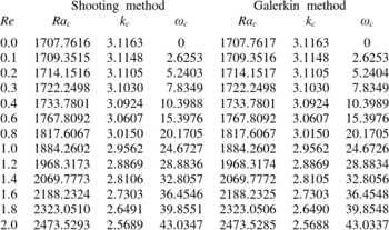
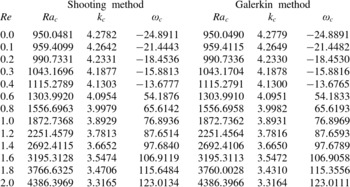
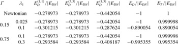
terms, which can be considered enough for convergence in all cases. Such a comparison is presented in table 1 for weakly elastic solutions and in table 2 for strongly elastic solutions. The definitions of weakly and strongly elastic solutions are given in § 4, which also provides the background to justify the cases selected to be analysed in the present study. Regardless, these tables show only small deviations, in the fourth digit at most, for all critical numbers at the Reynolds numbers considered. The shooting method can be considered accurate.
Critical parameters for a weakly elastic fluid at the onset of convective instability:
 $\mathit{Pr}=10$
,
 ${\it\lambda}_{1}=0.025$
and
 ${\it\Gamma}=0.15$
.

Critical parameters for a strongly elastic fluid at the onset of convective instability:
 $\mathit{Pr}=10$
,
 ${\it\lambda}_{1}=0.1$
and
 ${\it\Gamma}=0.15$
.

3.4. Spatio-temporal stability analysis
Once the onset of convective instability
 $\mathit{Ra}_{c}$
has been identified as a function of the control parameters
 $(\mathit{Re},\mathit{Pr},{\it\lambda}_{1},{\it\Gamma})$
, it is also important to determine the onset of absolute instability
 $\mathit{Ra}_{A}(\mathit{Re},\mathit{Pr},{\it\lambda}_{1},{\it\Gamma})$
as well. If both onsets coincide, the fluid flow transitions from stable to absolutely unstable directly. Otherwise, there will be a finite region of convective instability in the control parameter space, i.e.
 $\mathit{Ra}_{A}(\mathit{Re},\mathit{Pr},{\it\lambda}_{1},{\it\Gamma})>\mathit{Ra}_{c}(\mathit{Re},\mathit{Pr},{\it\lambda}_{1},{\it\Gamma})$
, between stable and absolutely unstable regions. Since the flow behaviour is dramatically different in each region, it is vital to identify these boundaries.
At the onset of absolute instability the dispersion relation
 $\mathfrak{D}({\it\omega}_{0},k_{0},\mathit{Ra},\mathit{Re},\mathit{Pr},$
 ${\it\lambda}_{1},{\it\Gamma})=0$
must be satisfied, as well as the mathematical necessary conditions (Huerre & Monkewitz Reference Huerre and Monkewitz1985; Brevdo Reference Brevdo1991)
 $$\begin{eqnarray}\left.\frac{\text{d}{\it\omega}}{\text{d}k}\right|_{k_{0}}=0\quad \text{and}\quad {\it\omega}_{i}(k_{0})=0,\end{eqnarray}$$
which is true only for a two-dimensional transition to absolute instability. Taking the derivative of the dispersion relation with respect to the wavenumber
 $k=k_{x}$
and applying conditions (3.16) to the result leads to the additional relation
 $$\begin{eqnarray}\left.\frac{\text{d}\mathfrak{D}({\it\omega},k,\mathit{Ra},\mathit{Re},\mathit{Pr},{\it\lambda}_{1},{\it\Gamma})}{\text{d}k}\right|_{k_{0}}=0.\end{eqnarray}$$
Real and imaginary parts of both relations (3.6) and (3.17) lead to a system of four equations that is able to generate initial estimates for the four unknowns
 ${\it\omega}_{r}^{0},\mathit{Ra}_{A},\text{Re}[k_{x}^{0}]$
and
 $\text{Im}[k_{x}^{0}]$
. Their existence might indicate a possible onset of absolute instability. This particular problem can also be solved with the built-in function FindRoot. However, due to the analytical nature of this algebraic system of equations, the Newton method is employed here instead and only one guess for each unknown is required. When applied to the same control parameters as utilized to generate figure 1, this method yields
 $$\begin{eqnarray}{\it\omega}_{A}\simeq 15.66,\quad \mathit{Ra}_{A}\simeq 523.2,\quad \text{Re}[k_{xA}]\simeq 3.414\quad \text{and}\quad \text{Im}[k_{xA}]\simeq -0.5481.\end{eqnarray}$$
Although necessary, condition (3.17) is not sufficient for the critical points it generates, such as (3.18), to represent a transition to absolute instability. In addition, one must verify that the spatial branches in the complex-
 $k$
plane, which are solutions of the dispersion relation
 $\mathfrak{D}=0$
, satisfy the Briggs–Bers collision criterion (Briggs Reference Briggs1964). This criterion dictates that all the spatial branches involved in the pinching process at the saddle point must originate from different imaginary half-planes in a complex-wavenumber map. Hence, we search for pinching points through the behaviour of their spatial branches. In other words, the parameters to be determined by the shooting method become
 $\mathscr{P}_{1}=\text{Re}[k_{x}]$
and
 $\mathscr{P}_{2}=\text{Im}[k_{x}]$
. Such a calculation is performed for fixed values of
 ${\it\omega}_{r}$
and
 $\mathit{Ra}$
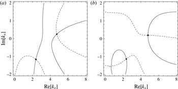
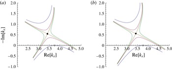
, in addition to the remaining control parameters. A procedure similar to the one used in the temporal stability analysis is repeated here to generate estimates for the shooting method. They are obtained by identifying where the dispersion relation lines with zero real and imaginary values intersect. Figure 2(a) presents these lines using (3.6) for
 $\mathit{Re}=0,\mathit{Pr}=10,{\it\lambda}_{1}=0.3$
and
 ${\it\Gamma}=0.15$
at
 ${\it\omega}_{r}=20$
and
 $\mathit{Ra}=511$
, which is a point near (3.18). Two modes are found,
 $k_{x}\simeq 4.732+0.2541\text{i}$
and
 $2.388-1.16\text{i}$
.
Now, these mode estimates are improved upon using a new shooting method variation. It first modifies
 $\mathfrak{F}_{2}$
into the new function
 $\mathfrak{F}_{3}$
, which receives
 $\text{Re}[k_{x}]$
and
 $\text{Im}[k_{x}]$
as input variables instead of
 ${\it\omega}_{r}$
and
 $\mathit{Ra}$
. It then solves (3.15) in the same way as explained before in § 3.3, but using
 $\mathfrak{F}_{3}$
instead of
 $\mathfrak{F}_{2}$
. Figure 2(b) presents the respective lines for this differential dispersion relation for the same parameters in as figure 2(a). These two modes appear once again, but with slightly different values in conjunction with their respective constants
 $\mathfrak{C}_{1}$
and
 $\mathfrak{C}_{2}$
. This improved estimate is then provided to the original shooting method, which yields the modes
 $k_{x}\simeq 4.798+0.1979\text{i}$
and
 $2.364-1.137\text{i}$
. Both branches are now constructed by varying
 ${\it\omega}_{r}$
at the same
 $\mathit{Ra}$
. However, this overall procedure is repeated for one additional
 ${\it\omega}_{r}$
only. From this point on, linear, quadratic and cubic extrapolations are consecutively employed, stopping at the latter one, as the data set increases to generate new estimates. The Briggs–Bers criterion as well as the pinching point are then identified through the behaviour of these spatial branches with respect to
 $\mathit{Ra}$
.
Figure 3 shows the behaviour of both spatial branches within
 $20\geqslant {\it\omega}_{r}\geqslant 10$
at four different Rayleigh numbers, obtained from both algebraic and differential dispersion relations in figures 3(a) and 3(b), respectively. The dominant mode in question is the bottom one in both plots, where the lowest curve is generated at
 $\mathit{Ra}=\mathit{Ra}_{c}$
and the grey dot shows the critical point in each plot. As the Rayleigh number is increased a little further, this mode crosses into the upper complex-half-plane and becomes convectively unstable. By increasing the Rayleigh number further, two spatial branches pinch when the saddle-point value is reached (the black dot locates the pinching point for
 $\mathit{Ra}=\mathit{Ra}_{A}$
). Since the collision criterion was satisfied, this point indeed represents a transition to absolute instability. The differential dispersion relation yields
 $k_{xA}\simeq 3.42-0.5607\text{i}$
, which is obtained by interpolating the closest point between spatial branches as soon as the pinching is observed, with an error of
 ${\rm\Delta}\mathit{Ra}=\pm 0.5$
. Although critical points in each plot are different, this difference is small and the qualitative mode behaviour is similar. Hence, the single-term Galerkin expansion does provide a valuable initial estimate for the onset of absolute instability as well.
Spatially unstable modes (solid points) for
 $\mathit{Re}=0,\mathit{Pr}=10,{\it\lambda}_{1}=0.3$
and
 ${\it\Gamma}=0.15$
with
 ${\it\omega}_{r}=20$
and
 $\mathit{Ra}=511$
. Solid lines represent
 $\text{Re}[\mathfrak{D}]=0$
whereas dashed lines represent
 $\text{Im}[\mathfrak{D}]=0$
according to: (a) algebraic dispersion relation (3.6) from single-term Galerkin expansion and (b) differential dispersion relation (3.15) solved with the shooting method variation.

Behaviour of the two spatial branches shown in figure 2 for different Rayleigh numbers within
 $20\geqslant {\it\omega}_{r}\geqslant 10$
. Grey and black points represent the onset of convective and absolute instabilities, respectively. (a) Algebraic dispersion relation (3.6) data at
 $\mathit{Ra}=495.97$
, 520, 523.19 and 526 and (b) differential dispersion relation (3.15) data at
 $\mathit{Ra}=484.57$
, 509, 512 and 515.

Another attempt was made to verify the shooting method accuracy, this time for the onset of absolute instability, by comparing it with the Galerkin method. However, the computational time required for the derivation of relation (3.17), which is subjected to condition (3.16), also known as zero group velocity condition, from algebraic dispersion relation (3.5) dramatically increases with the number of terms
 $N$
. Hence, we were not able to generate results for
 $N>3$
within an acceptable computational time. Nevertheless, figures 2 and 3 provide enough proof of the shooting method accuracy for this onset.
3.5. Test case in relation to experiments
As we were confronted by a lack of published results on RBP mixed convection for viscoelastic fluids, we first test the validity of our numerical scheme against the results of Nicolas et al. (Reference Nicolas, Mojtabi and Platten1997) and Carrière & Monkewitz (Reference Carrière and Monkewitz1999) obtained in the limiting case of Newtonian fluids.
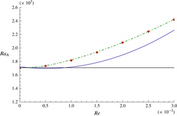
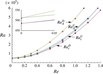
In figure 4 we compare our results (symbols) – corresponding to the transition curve from convective to absolute instability of TRs in the Reynolds–Rayleigh number plane – with the results computed by Carrière & Monkewitz (Reference Carrière and Monkewitz1999) using a Chebyshev collocation method (dash-dotted line). Both results are obtained for
 $\mathit{Pr}=450$
. Also included in figure 4 is the quadratic fit (solid line) of the experimental measurements of the convective–absolute transition of TRs conducted by Grandjean & Monkewitz (Reference Grandjean and Monkewitz2009) with oil as a working fluid, namely,
 $$\begin{eqnarray}\mathit{Ra}_{A}=9.296\times 10^{5}\mathit{Re}^{2}-9.897\times 10^{3}Re+1.723\times 10^{3}.\end{eqnarray}$$
As can be seen from the figure, our results are in very good agreement with the numerical computation of Carrière & Monkewitz (Reference Carrière and Monkewitz1999). Nevertheless, this figure reveals that the experimental convective–absolute transition curve lies below the theoretical curves. This difference was already noticed by Grandjean & Monkewitz (Reference Grandjean and Monkewitz2009) and was attributed by these authors to the finite heat diffusivity of the boundaries of the experimental cell.
Stability boundaries of the convective–absolute transition of TRs for mineral oil (
 $\mathit{Pr}=450$
). Symbols represent results of the present work compared with that computed numerically (dash-dotted line) by Carrière & Monkewitz (Reference Carrière and Monkewitz1999), while the solid line is a least-square quadratic fit (3.19) of the experimental work conducted by Grandjean & Monkewitz (Reference Grandjean and Monkewitz2009). The horizontal line represents the well-known threshold for RB instability,
 $\mathit{Ra}=1707.762$
(Chandrasekhar Reference Chandrasekhar1961).

Nicolas et al. (Reference Nicolas, Mojtabi and Platten1997) reported results on the properties of TRs obtained by a two-dimensional direct numerical simulation (DNS) of the RBP problem for
 $\mathit{Pr}=6.4$
. For a Reynolds number
 $\widetilde{Re}$
based on the average base flow velocity such that
 $\widetilde{Re}<0.21$
(
 $\widetilde{Re}>0.21$
), they found that the oscillation frequency of TRs decreases (increases) when Rayleigh number increases. At
 $\widetilde{Re}=0.21$
, the frequency remained constant for all Rayleigh numbers employed. Qualitatively, this finding compares well with the experimental data obtained by laser-Doppler anemometry (LDA) measurements in Ouazzani, Platten & Mojtabi (Reference Ouazzani, Platten and Mojtabi1990) with water as the working fluid. In the present work we found that the dimensionless frequency of TR oscillations computed for
 $\mathit{Pr}=6.4$
at the absolute instability threshold is
 ${\it\omega}_{A}=5.41$
at
 $\mathit{Re}=0.315$
which corresponds to
 $\widetilde{Re}=0.21$
(note the factor of 1.5 between
 $\widetilde{Re}$
and the current Reynolds number based on the maximum base flow velocity). This frequency can be expressed in dimensional form by using the scaling factor
 $h^{2}/K$
with
 $h=4.15~\text{mm}$
and
 $K=0.145~\text{mm}^{2}~\text{s}^{-1}$
(Ouazzani et al.
Reference Ouazzani, Platten and Mojtabi1990). In table 3 we compare the dimensional oscillation frequencies of TRs at the absolute instability threshold, and for
 $\mathit{Re}=0.315$
, obtained by our theoretical prediction, DNS results (Nicolas et al.
Reference Nicolas, Mojtabi and Platten1997), and experimental measurements (Ouazzani et al.
Reference Ouazzani, Platten and Mojtabi1990). Table 3 demonstrates that our computed frequency at the onset of absolute instability of TRs compares well with the value obtained by DNS. The discrepancy between the two values is 1.4 %. Also, table 3 reveals that the results of the present work and of the DNS tend to overestimate the oscillation frequency.
Validation of our numerical scheme against the results in Ouazzani et al. (Reference Ouazzani, Platten and Mojtabi1990) and Nicolas et al. (Reference Nicolas, Mojtabi and Platten1997), for
 $\mathit{Pr}=6.4$
.

4. Review of the linear stability in the absence of throughflow
Before discussing throughflow effects on viscoelastic instabilities, an overview of linear stability results in the absence of throughflow is presented. Li & Khayat (Reference Li and Khayat2005) distinguish two different regimes in this limit, i.e. when
 $\mathit{Re}=0$
. The so-called weakly elastic regime corresponds to the parameter set where the conductive base state first bifurcates to a stationary convective state. Otherwise, in the strongly elastic regime, the onset of convection is oscillatory. Approximate results for both regimes can be generated with algebraic dispersion relation (3.6), obtained from a single-term Galerkin expansion. The marginal stability curve for the onset of stationary convection is independent of viscoelastic parameters. It is same as obtained for Newtonian fluids, given by
 $$\begin{eqnarray}\mathit{Ra}^{s}=\frac{28}{27}\frac{f_{1}\,f_{4}}{k^{2}},\end{eqnarray}$$
which yields the critical values
 $\mathit{Ra}_{c}^{s}=1749.98$
and
 $k_{c}^{s}=3.11652$
. The same is not true for the onset of oscillatory convection, since Kolka & Ierley (Reference Kolka and Ierley1987) have shown that
 $$\begin{eqnarray}\mathit{Ra}^{o}=\mathit{Ra}^{s}-\frac{28{\it\omega}^{2}}{27k^{2}}\left[\frac{f_{2}}{\mathit{Pr}}-\frac{{\it\lambda}_{1}\,f_{4}(1-{\it\Gamma})(1-{\it\lambda}_{1}\,f_{1})}{1+{\it\lambda}_{1}^{2}{\it\omega}^{2}}\right],\end{eqnarray}$$
where the frequency
 ${\it\omega}$
of the oscillatory mode is obtained from
 $$\begin{eqnarray}{\it\omega}^{2}=\frac{1}{{\it\lambda}_{1}^{2}}\left(({\it\lambda}_{1}\,f_{1}(1-{\it\Gamma})-1)f_{4}-\frac{f_{1}\,f_{2}}{\mathit{Pr}}\right)\Big/\left({\it\Gamma}f_{4}+\frac{f_{1}\,f_{2}}{\mathit{Pr}}\right),\end{eqnarray}$$
since both the critical Rayleigh number
 $\mathit{Ra}_{c}^{o}$
and critical wavenumber
 $k_{c}^{o}$
for the onset of oscillatory convection depend on the viscoelastic parameters
 ${\it\lambda}_{1}$
and
 ${\it\Gamma}$
, as well as
 $\mathit{Pr}$
.
Using the above results, it is possible to estimate the parameter set that locates the boundary separating weakly and strongly elastic regimes. For fixed values of
 ${\it\Gamma}$
and
 $\mathit{Pr}$
, there exists a value of
 ${\it\lambda}_{1}={\it\lambda}_{1}^{f}$
where
 $\mathit{Ra}_{c}^{s}=\mathit{Ra}_{c}^{o}$
. In other words, the critical Rayleigh numbers for the onsets of both stationary and oscillatory convection coincide at well-defined parametric conditions and, therefore, a codimension-two bifurcation occurs. Furthermore, as shown by Martinez-Mardones & Perez-Garcia (Reference Martinez-Mardones and Perez-Garcia1990) as well as Li & Khayat (Reference Li and Khayat2005),
 ${\it\lambda}_{1}^{f}$
decreases with an increasing
 $\mathit{Pr}$
for a fixed
 ${\it\Gamma}$
. In the limiting case of
 ${\it\Gamma}\rightarrow 0$
(Maxwell fluid) and
 $Pr\rightarrow \infty$
,
 ${\it\lambda}_{1}^{f}$
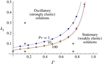
reaches the minimum value of 0.039. This behaviour is illustrated in figure 5, which shows
 ${\it\lambda}_{1}^{f}$
isolines on a (
 ${\it\Gamma},{\it\lambda}_{1}$
) plane for different values of
 $\mathit{Pr}$
obtained from the single-term Galerkin expansion (3.6). These studies guided our selection of test cases to investigate how the presence of throughflow affects both weakly and strongly elastic solutions. Three cases for each solution type plus a Maxwell fluid were analysed, and they are marked with asterisks in figure 5. Each case is correlated with one or two more cases, enabling a qualitative trend analysis. Furthermore, throughout this paper we shall assume
 $\mathit{Pr}=10$
unless stated otherwise.
Elasticity levels
 ${\it\lambda}_{1}^{f}$
defining the crossover between stationary (weakly elastic) and oscillatory (strongly elastic) bifurcations, for
 $\mathit{Re}=0$
and
 $\mathit{Pr}=1$
, 10 and 100. Results were obtained with the single-term Galerkin expansion (3.6). Stars indicate representative pairs of
 $({\it\Gamma},{\it\lambda}_{1})$
used in computations throughout the paper.

It should also be pointed out that the influence of fluid elasticity
 ${\it\lambda}_{1}$
on pattern selection without throughflow has been studied using nonlinear analysis as well. Li & Khayat (Reference Li and Khayat2005) investigated the onset of stationary instabilities in the weakly elastic regime, focusing on steady hexagon and square patterns. On the other hand, Martinez-Mardones et al. (Reference Martinez-Mardones, Tiemann, Walgraef and Zeller1996) investigated Hopf bifurcations in the strongly elastic regime, demonstrating that time-periodic patterns selected by nonlinear effects correspond to standing waves.
5. Temporal stability approach
After this brief discussion of the main thermal instability mechanisms that exist for viscoelastic fluids in the absence of throughflow, its effect can now be properly studied. When doing so, weakly and strongly elastic regimes are analysed separately through an appropriate selection of elasticity
 ${\it\lambda}_{1}$
and viscosity ratio
 ${\it\Gamma}$
pairs for
 $\mathit{Pr}=10$
, as discussed in the previous section, and for a wide range of Rayleigh and Reynolds numbers:
 $\mathit{Ra}\leqslant 8000$
and
 $\mathit{Re}\leqslant 2$
. Here, the Reynolds number
 $\mathit{Re}$
is increased from zero to uncover the effect of throughflow. The onset of convective instability is determined first using a temporal stability analysis, since critical spatial growth rates are zero at this onset. In other words, perturbations can be decomposed into normal modes with complex frequencies and real wavenumbers.
As argued before, LRs (
 $k_{x}=0$
,
 $k=k_{y}$
), which are helicoidal rolls with their axes parallel to the throughflow direction, are not affected by the throughflow. Their instability characteristics are the same as those obtained without throughflow (
 $\mathit{Re}=0$
). Hence, they appear as stationary rolls in the weakly elastic regime and oscillatory rolls in the strongly elastic regime. In the latter case, the marginal curve and associated frequency are given by (4.2) and (4.3), respectively, according to the approximate dispersion equation. Since these results are already known, the remainder of the section focuses on linear properties of TRs (
 $k_{x}=k$
,
 $k_{y}=0$
), whose axes are perpendicular to the throughflow direction. The characteristics of three-dimensional ORs can be easily deduced from TRs using the inverse Squire transformation.
5.1. Results for weakly elastic fluids
We first consider the transition from stable to convectively unstable regimes of weakly elastic fluids. In the framework of approximate algebraic dispersion relation (3.6), the following analytical results are obtained for TRs:
 $$\begin{eqnarray}{\it\omega}^{(TRs)}(k,\mathit{Re},\mathit{Pr},{\it\lambda}_{1},{\it\Gamma})=k\mathit{Re}\,\mathit{Pr}\,F(k^{2},\mathit{Pr},{\it\lambda}_{1},{\it\Gamma}),\end{eqnarray}$$
and
 $$\begin{eqnarray}\mathit{Ra}^{(TRs)}(k^{2},\mathit{Re},\mathit{Pr},{\it\lambda}_{1},{\it\Gamma})-\mathit{Ra}(\mathit{Re}=0)={\textstyle \frac{4}{27}}\mathit{Re}^{2}\mathit{Pr}{\it\Phi}(k^{2},\mathit{Pr},{\it\lambda}_{1},{\it\Gamma}),\end{eqnarray}$$
with additional functions defined as
 $$\begin{eqnarray}F(k^{2},\mathit{Pr},{\it\lambda}_{1},{\it\Gamma})=\frac{{\textstyle \frac{6}{7}}\mathit{Pr}\,f_{4}+{\textstyle \frac{2}{11}}f_{1}\,f_{3}-\mathit{Pr}f_{1}\,f_{5}{\it\lambda}_{1}(1-{\it\Gamma})}{\mathit{Pr}\,f_{4}+f_{1}\,f_{2}-\mathit{Pr}f_{1}\,f_{4}{\it\lambda}_{1}(1-{\it\Gamma})},\end{eqnarray}$$
and
 $$\begin{eqnarray}\displaystyle {\it\Phi}(k^{2},\mathit{Pr},{\it\lambda}_{1},{\it\Gamma}) & = & \displaystyle (7F-6)({\textstyle \frac{2}{11}}\,f_{3}-f_{2}\,F-\mathit{Pr}\,f_{4}F{\it\lambda}_{1}(1+{\it\Gamma})\mathit{Pr}-\mathit{Pr}f_{5}{\it\lambda}_{1}(1-{\it\Gamma}))\nonumber\\ \displaystyle & & \displaystyle +\,7f_{1}\,F{\it\lambda}_{1}({\textstyle \frac{4}{11}}\,f_{3}-2\,f_{2}\,F+\mathit{Pr}\,f_{4}F{\it\lambda}_{1}(1-{\it\Gamma})),\end{eqnarray}$$
where a close inspection of (5.1) and (5.2) reveals that these expressions for
 ${\it\omega}^{(TRs)}$
and
 $\mathit{Ra}^{(TRs)}$
coincide exactly with equations (4.2) and (4.3) from Carrière & Monkewitz (Reference Carrière and Monkewitz1999) in the limiting case of Newtonian fluids (
 ${\it\Gamma}=1$
).
Since throughflow has a weak effect on the critical wavenumber in the limit of a small product
 ${\it\lambda}_{1}\mathit{Re}\mathit{Pr}$
, we set
 $k_{c}^{(TRs)}=k_{c}^{s}(\mathit{Re}=0)=3.11652$
and derive a simple formula for the marginal TR frequency, given by
 $$\begin{eqnarray}{\it\omega}_{c}^{(TRs)}=\mathit{Re}\mathit{Pr}\frac{0.9480+2.6713\mathit{Pr}-55.4647\mathit{Pr}{\it\lambda}_{1}(1-{\it\Gamma})}{0.5148+\mathit{Pr}-19.7126\mathit{Pr}{\it\lambda}_{1}(1-{\it\Gamma})},\end{eqnarray}$$
which is zero at
 $\mathit{Re}=0$
. This expression indicates that the critical frequency grows linearly with Reynolds number, since the rate of change
 $\partial {\it\omega}_{c}^{(TRs)}/\partial Re$
is found to be positive for all combinations (
 ${\it\Gamma},{\it\lambda}_{1}$
) in the weakly elastic regime. Furthermore, the expression for
 ${\it\omega}_{c}^{(TRs)}$
given by Carrière & Monkewitz (Reference Carrière and Monkewitz1999) is recovered from (5.5) when
 ${\it\Gamma}=1$
.
Based on the above results, the dimensionless critical phase velocity is given by
 $$\begin{eqnarray}\frac{V_{{\it\varphi}}^{\ast }}{U_{0}^{\ast }}=\frac{{\it\omega}_{c}^{(TRs)}}{k_{c}^{(TRs)}}\frac{1}{\mathit{Re}\mathit{Pr}},\end{eqnarray}$$
using the base flow length and time scales for
 $V_{{\it\varphi}}^{\ast }$
on the left-hand side of (5.6) but their perturbation counterparts on its right-hand side. Since this phase velocity is positive, the travelling wave induced by the presence of throughflow propagates in the downstream direction. With
 $\mathit{Pr}=10$
imposed in this study, one finds
 $V_{{\it\varphi}}^{\ast }/U_{0}=0.844$
in the limit of
 ${\it\Gamma}=1$
. It compares well with the value of 0.867 obtained numerically by Nicolas, Luijks & Platten (Reference Nicolas, Luijks and Platten2000) (see table 5 of that paper and note the factor of 1.5 between their Reynolds number based on the average base flow velocity and the current Reynolds number based on the maximum base flow velocity). The relative difference between the two numbers is 2.6 %. The effect of rheological parameters
 ${\it\lambda}_{1}$
and
 ${\it\Gamma}$
on
 $V_{{\it\varphi}}^{\ast }/U_{0}^{\ast }$
will be discussed later in this section.
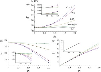
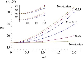
Having used the approximate dispersion relation to provide initial estimates of the throughflow influence, converged results are generated by applying the shooting method to the full dispersion relation and are analysed in detail next. Figure 6 shows critical stability curves for the Rayleigh number, wavenumber and oscillation frequency as functions of the Reynolds number for
 ${\it\lambda}_{1}=0.025$
and different values of
 ${\it\Gamma}$
. It can be observed from these figures that, in the absence of throughflow (
 $\mathit{Re}=0$
), the weak elasticity of the fluid does not influence the onset of convective instability and the critical values
 $\mathit{Ra}_{c},k_{c}$
and
 ${\it\omega}_{c}$
are the same as those of a Newtonian fluid (
 ${\it\Gamma}=1$
). As expected in this case, a pitchfork bifurcation is observed for all
 ${\it\Gamma}$
, even in the limiting case of a Maxwell fluid (
 ${\it\Gamma}=0$
), also presented for comparison purposes.
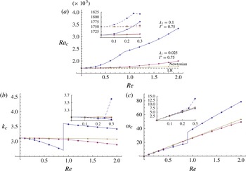
Critical (a) Rayleigh number, (b) wavenumber, and (c) oscillation frequency at the onset of convective instability for weakly elastic TRs with
 ${\it\lambda}_{1}=0.025$
and different values of
 ${\it\Gamma}$
, including the Newtonian fluid case (
 ${\it\Gamma}=1$
). The threshold of LRs (dashed line) is also presented. TR comparisons between full dispersion relation (solid lines) and approximate dispersion relation (dashed lines) are shown in the insets.

At any given finite but non-vanishing throughflow (
 $\mathit{Re}\neq 0$
), it is clear from figure 6(a) that an increase in
 ${\it\Gamma}$
leads to flow destabilization, i.e. to a reduction in the respective critical Rayleigh number. The least unstable condition corresponds to a Maxwell fluid (
 ${\it\Gamma}=0$
) whereas the most unstable one corresponds to a Newtonian fluid (
 ${\it\Gamma}=1$
). It is important to note that an opposite trend has been observed in a porous medium by Hirata & Ouarzazi (Reference Hirata and Ouarzazi2010). Such a qualitative difference in behaviour with respect to the viscosity ratio is likely to be due to the linear character of Darcy’s law, used to model the momentum equations in the porous medium.
Figure 6(a) also shows the stabilizing effect of throughflow for any fixed value of the viscosity ratio. The critical Rayleigh number at the onset of convective instability
 $\mathit{Ra}_{c}$
for the Newtonian fluid case (
 ${\it\Gamma}=1$
) only shows a weak dependence on
 $\mathit{Re}$
. However, as the viscosity ratio
 ${\it\Gamma}$
decreases, the throughflow stabilization increases. In other words,
 $\mathit{Ra}_{c}$
is an increasing function of
 $\mathit{Re}$
. Furthermore, the smaller the value of
 ${\it\Gamma}$
, the more pronounced is this effect. Figure 6(b) on the other hand, shows a decrease in critical wavenumber
 $k_{c}$
with increasing
 $\mathit{Re}$
as well as decreasing
 ${\it\Gamma}$
, both in the weakly elastic regime. This implies that emerging transversal convection rolls have a larger cross-section when the throughflow is moderate and/or the polymer concentration is high. The dependence of the critical oscillatory frequency
 ${\it\omega}_{c}$
on
 $\mathit{Re}$
is shown in figure 6(c). Its value decreases with decreasing
 ${\it\Gamma}$
, although this effect is nearly negligible at small
 $\mathit{Re}$
. The dimensionless critical phase velocity
 $V_{{\it\varphi}}^{\ast }/U_{0}^{\ast }$
, averaged over the range of Reynolds numbers shown in this figure, varies from 0.83 for Maxwellian fluids (
 ${\it\Gamma}=0$
) to 0.86 for Newtonian fluids (
 ${\it\Gamma}=1$
). Hence, the addition of polymer molecules to a solution with very weak elasticity has no significant effect on the phase velocity of TRs.
Finally, the insets in figure 6 show comparisons between the converged numerical results obtained from the full dispersion relation using a shooting method and the approximate analytical results obtained from the algebraic dispersion relation generated using a single-term Galerkin expansion. A fairly good agreement is observed for low values of the Reynolds number. Approximate results are in qualitative agreement with converged ones, where an excellent quantitative agreement is observed up to
 $\mathit{Re}\leqslant 0.3$
, with a maximum relative error for
 $\mathit{Ra}_{c}$
smaller than 2.5 %. When the Reynolds number exceeds
 $\mathit{Re}=0.3$
, the approximate results start to significantly diverge from the converged numerical ones.
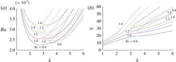
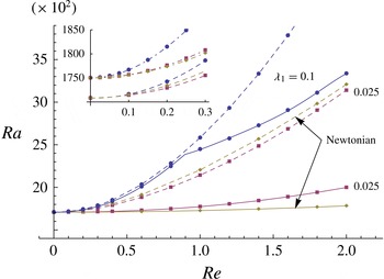
It is now possible to study the influence of fluid elasticity by considering the throughflow dependence at a higher value of
 ${\it\lambda}_{1}$
for a fixed value of
 ${\it\Gamma}$
. Figure 7 presents results for
 ${\it\lambda}_{1}=0.1$
and
 ${\it\Gamma}=0.75$
, a typical viscosity ratio value for Boger fluids. Curves for the critical parameters at
 ${\it\lambda}_{1}=0.025$
and
 ${\it\Gamma}=0.75$
as well as the Newtonian case (
 ${\it\Gamma}=1$
) are also presented for comparison purposes. Figure 7(a) shows that for
 $\mathit{Re}=0$
, once again, the first bifurcation to occur is stationary (
 ${\it\omega}_{c}=0$
) and the critical Rayleigh number is the same as the one derived for Newtonian fluids. Furthermore, it is now clear that an increase in fluid elasticity strongly increases the stabilization of the base state against TRs when
 $\mathit{Re}\neq 0$
. On the other hand, a qualitative difference is observed between figures 6 and 7, where discontinuities appear when increasing
 $\mathit{Re}$
. Figure 7(a) shows a discontinuity in the first derivative of
 $\mathit{Ra}_{c}$
whereas figure 7(b,c) shows a discontinuity in the functions
 $k_{c}$
and
 ${\it\omega}_{c}$
themselves, respectively. The critical wavenumber decreases with an increase in
 $\mathit{Re}$
, but jumps to a larger value at approximately
 $\mathit{Re}\simeq 0.9$
. Nevertheless, it still decreases with an increase in
 $\mathit{Re}$
beyond this point. The critical frequency always increases with an increase in
 $\mathit{Re}$
, initially with a slope similar to the Newtonian fluid case, but jumps to a higher value at
 $\mathit{Re}\simeq 0.9$
. Consequently, a jump in the average value of
 $V_{{\it\varphi}}^{\ast }/U_{0}^{\ast }$
is also observed, from 0.8 to 1.13. This increase in dimensionless phase velocity when
 $\mathit{Re}\gtrsim 0.9$
means that a downstream moving most unstable TR becomes faster than the base flow that feeds energy to it. Finally, the insets shown in figure 7 provide a similar comparison between approximate and full dispersion relation results to that shown in figure 6. There is good qualitative and quantitative agreement, but only up to
 $\mathit{Re}\lesssim 0.25$
, where the maximum relative error for
 $\mathit{Ra}_{c}$
is smaller than 3.46 %. However, it is important to mention that the Reynolds number where the discontinuity is located is poorly predicted by the approximate algebraic dispersion relation.
Critical (a) Rayleigh number, (b) wavenumber and (c) oscillation frequency at the onset of convective instability for weakly elastic TRs with
 ${\it\lambda}_{1}=0.1$
and
 ${\it\Gamma}=0.75$
. The Newtonian fluid case as well as the
 ${\it\lambda}_{1}=0.025$
and
 ${\it\Gamma}=0.75$
case are also presented. TR comparisons between full dispersion relation (solid lines) and approximate dispersion relation (dashed lines) are shown in the insets. Codimension-two bifurcation at
 $\mathit{Re}_{c2}=0.896791$
.

Neutral stability curves in the (a)
 $(k,\mathit{Ra})$
and (b)
 $(k,{\it\omega})$
planes for different values of the Reynolds number
 $\mathit{Re}$
with
 ${\it\lambda}_{1}=0.1$
and
 ${\it\Gamma}=0.75$
. They show the presence of two convectively unstable modes as solid and dashed lines.

In order to uncover the origin of this discontinuity, neutral stability curves in the
 $(k,\mathit{Ra})$
and
 $(k,{\it\omega})$
planes are displayed in figure 8, for different values of the Reynolds number around
 $\mathit{Re}=1$
with
 ${\it\lambda}_{1}=0.1$
and
 ${\it\Gamma}=0.75$
. Two modes can be distinguished in these figures, where the first one is represented by a parabolic-shaped curve and the second one by a finger-shaped curve. The neutral stability curve associated with the first mode in figure 8(a) is a traditional one, where the temporal growth rate associated with this mode is negative below it and positive above it. On the other hand, a different behaviour is observed for the second mode in the same figure. This mode is amplified inside its neutral stability curve and damped outside it. Hence, two minima exist, one for each curve, and they compete for the position of global minimum. The first mode is the most unstable one when
 $\mathit{Re}=0.8$
, with the global minimum located at
 $\mathit{Ra}_{c}=2246.07,k_{c}=2.77644$
and
 ${\it\omega}_{c}=17.4039$
. However, it is the second mode that yields a global minimum when
 $\mathit{Re}=1.0$
, which is located at
 $\mathit{Ra}_{c}=2447,k_{c}=3.58395$
and
 ${\it\omega}_{c}=39.1393$
. Hence, a codimension-two bifurcation exists and occurs at
 $\mathit{Re}_{c2}=0.896791$
, which is the Reynolds number at which the two modes are equally unstable. This switch between modes is responsible for the discontinuities observed in figure 7. It appears to be due to the higher value of the fluid elasticity. The physical mechanisms behind the transition between these two unstable modes are elucidated by the energy analysis performed in § 5.3.2.
5.2. Results for strongly elastic fluids
The onset of convective instability is now addressed for strongly elastic solutions. A detailed discussion of the
 ${\it\lambda}_{1}=0.3$
and
 ${\it\Gamma}=0.75$
case is provided first. Three bifurcating convective solutions exist. Their respective bifurcation thresholds and critical frequencies are presented in figure 9. In the absence of throughflow
 $(\mathit{Re}=0)$
, the numerically obtained threshold of stationary convection is
 $\mathit{Ra}_{c}^{s}=1707.76$
. On the other hand, the Hopf bifurcation threshold for the same Reynolds number is
 $\mathit{Ra}_{c}^{o}=1574.77$
for symmetry-degenerate right or left propagating travelling waves with opposite critical Hopf frequencies
 ${\it\omega}_{c}=\pm 2.68$
. Since
 $\mathit{Ra}_{c}^{o}<\mathit{Ra}_{c}^{s}$
in the absence of throughflow, the system undergoes a Hopf bifurcation, which characterizes it as strongly elastic.
(a) Critical Rayleigh number and (b) critical frequency for the three modes of instability in a strongly elastic solution (
 ${\it\lambda}_{1}=0.3$
and
 ${\it\Gamma}=0.75$
) as a function of the Reynolds number. The superscripts
 $S$
,
 $D$
and
 $U$
refer to the stationary, downstream and upstream mode respectively. The inset in (a) shows that the critical Rayleigh curves of the upstream and downstream modes intersect at
 $\mathit{Re}=\mathit{Re}_{c2}\simeq 0.6$
.

The presence of throughflow breaks the mirror symmetry (
 $x\rightarrow -x$
), but the selection process differs from that observed for weakly elastic solutions. In order to distinguish between the three unstable modes for
 $\mathit{Re}>0$
, we use superscripts
 $S$
,
 $U$
and
 $D$
. The superscript
 $S$
characterizes the stationary unstable mode in the
 $\mathit{Re}=0$
limit, i.e.
 ${\it\omega}_{c}(\mathit{Re}\rightarrow 0)=0$
. The superscript
 $D$
(
 $U$
) identifies the mode for which
 ${\it\omega}_{c}(\mathit{Re}\rightarrow 0)$
is positive (negative) and the associated travelling waves will be denoted TWD (TWU). As shown in figure 9(a), the three patterns yield three different values of the critical Rayleigh number that evolve differently with
 $\mathit{Re}$
. The stabilizing effect of throughflow is found more important for the
 $S$
mode than for TWD and TWU modes. The most critical Rayleigh number corresponds either to
 $\mathit{Ra}_{c}^{D}$
or to
 $\mathit{Ra}_{c}^{U}$
depending on Reynolds number. When
 $\mathit{Re}\lesssim 0.6$
, the TWU mode, which has
 ${\it\omega}_{c}<0$
when
 $\mathit{Re}=0$
(see figure 9
b), is the most unstable, i.e.
 $\mathit{Ra}_{c}^{U}<\mathit{Ra}_{c}^{D}$
. For larger
 $\mathit{Re}$
, as
 $\mathit{Ra}_{c}^{D}<\mathit{Ra}_{c}^{U}$
, a transition occurs from TWU to TWD. Hence, a codimension-two bifurcation point exists when
 $\mathit{Ra}_{c}^{U}=\mathit{Ra}_{c}^{D}$
and is in fact located at
 $\mathit{Re}_{c2}=0.603077$
. The transition from TWU to TWD is well illustrated in figure 10 for
 $\mathit{Re}=0.4$
, 0.6 and 0.8, where the parabolic shaped curve (solid line) and a finger shaped curve (dashed line) represent the neutral stability curves for TWU and TWD respectively. We emphasize that the observed transition is accompanied by a substantial jump in oscillation frequency, from
 ${\it\omega}_{c}=4.97404$
to 28.0336 and in wavenumber, from
 $k_{c}=3.0828$
to 3.23644, leading to a discontinuous change in phase speed. Such a jump leads to a significant increase in the average ratio
 $V_{{\it\varphi}}^{\ast }/U_{0}^{\ast }$
from 0.267539 to 1.43628, indicating that TWD travels faster than the maximum base flow velocity when
 $\mathit{Re}>\mathit{Re}_{c2}$
.
Neutral stability curves in the (a)
 $(k,\mathit{Ra})$
and (b)
 $(k,{\it\omega})$
planes for different values of the Reynolds number
 $\mathit{Re}$
with
 ${\it\lambda}_{1}=0.3$
and
 ${\it\Gamma}=0.75$
. The parabolic-shaped curve and finger-shaped curve represent the neutral stability curves for TWU and TWD respectively.

Having analysed in detail the
 ${\it\lambda}_{1}=0.3$
and
 ${\it\Gamma}=0.75$
case, it can now be used as a reference in the examination of the effects of the two viscoelastic parameters on the flow stability properties. In the remainder of this subsection, instead of presenting the three unstable modes, we focus solely on the properties of the most unstable one, which may be TWU or TWD depending on the rheological parameters and on the prescribed Reynolds number. In order to evaluate the effect of elasticity alone,
 ${\it\lambda}_{1}=0.1$
and
 ${\it\lambda}_{1}=0.3$
cases are investigated for a fixed
 ${\it\Gamma}=0.15$
. On the other hand, the effect of viscosity ratio alone is studied by fixing
 ${\it\lambda}_{1}=0.3$
and investigating the
 ${\it\Gamma}=0.15$
and
 ${\it\Gamma}=0.75$
cases. The four different cases are shown in figure 11, which represents the true critical Rayleigh number, wavenumber, oscillatory frequency and phase speed at the onset of convective instability. It includes all possible parameter combinations between
 ${\it\lambda}_{1}=0.1$
and 0.3 and
 ${\it\Gamma}=0.15$
and 0.75. It is important to note that the case with
 ${\it\lambda}_{1}=0.1$
and
 ${\it\Gamma}=0.75$
represents a weakly elastic solution and is included as a solid line without symbols for comparison purposes. As expected for strongly elastic solutions, a Hopf bifurcation occurs for all three combinations of rheological parameters in the limit of zero Reynolds number. In this limit, the critical Rayleigh numbers which mark the onset of oscillatory convective instability are
 $\mathit{Ra}_{c}^{o}=950.05$
for
 ${\it\lambda}_{1}=0.1$
and
 ${\it\Gamma}=0.15$
,
 $\mathit{Ra}_{c}^{o}=484.57$
for
 ${\it\lambda}_{1}=0.3$
and
 ${\it\Gamma}=0.15$
, and
 $\mathit{Ra}_{c}^{o}=1574.77$
for
 ${\it\lambda}_{1}=0.3$
and
 ${\it\Gamma}=0.75$
. This indicates that
 $\mathit{Ra}_{c}^{o}$
decreases with increasing
 ${\it\lambda}_{1}$
and increases with increasing
 ${\it\Gamma}$
when
 $\mathit{Re}=0$
. Such a respectively destabilizing/stabilizing role of these rheological parameters is maintained at non-zero but still low Reynolds numbers, but is reversed beyond a high enough Reynolds number. Figure 11(a) also shows the role reversal induced by both fluid elasticity and solute viscosity ratio in the cases being compared here, which occur at
 $\mathit{Re}=0.497597$
and 0.759447, respectively.
Two additional remarks about figure 11 are necessary. The first one is the absence of any discontinuities for the
 ${\it\lambda}_{1}=0.3$
and
 ${\it\Gamma}=0.15$
case. Secondly, for the other cases, the observed discontinuities induce a substantial change in the magnitude of the phase velocity. For instance, in the
 ${\it\lambda}_{1}=0.1$
and
 ${\it\Gamma}=0.15$
case, the average ratio
 $V_{{\it\varphi}}^{\ast }/U_{0}^{\ast }$
jumps from
 $-$
0.78829 to 2.54131 at
 $\mathit{Re}=\mathit{Re}_{c2}$
. In other words, the relative average phase velocity switches between almost two times the maximum base flow velocity travelling upstream, for
 $\mathit{Re}<\mathit{Re}_{c2}$
, to almost two times the same value but travelling downstream, for
 $\mathit{Re}>\mathit{Re}_{c2}$
.
Critical (a) Rayleigh number, (b) wavenumber, (c) oscillation frequency, and (d) phase speed at the onset of convective instability for strongly elastic TRs with
 ${\it\lambda}_{1}=0.3$
and
 ${\it\Gamma}=0.75$
(
 $\mathit{Re}_{c2}=0.603077$
),
 ${\it\lambda}_{1}=0.3$
and
 ${\it\Gamma}=0.15$
, as well as
 ${\it\lambda}_{1}=0.1$
and
 ${\it\Gamma}=0.15$
(
 $\mathit{Re}_{c2}=0.41291$
). Weakly elastic TRs with
 ${\it\lambda}_{1}=0.1$
and
 ${\it\Gamma}=0.75$
(solid lines without symbols) also presented.

Finally, it is important to note that critical Rayleigh numbers for three-dimensional disturbances (i.e. ORs), can be obtained from Squire transformation (3.14), i.e.
 $$\begin{eqnarray}\mathit{Ra}_{c}^{3D}(k_{x}^{2}+k_{y}^{2},k_{x}\mathit{Re}_{3D})={\mathit{Ra}_{c}}^{\!2D}(k^{2},k\mathit{Re})\quad \text{with}~\mathit{Re}_{3D}=(k/k_{x})\mathit{Re},\end{eqnarray}$$
which means a higher values of
 $\mathit{Re}_{3D}$
compared to
 $\mathit{Re}$
is required, since
 $k^{2}=k_{x}^{2}+k_{y}^{2}>k_{x}^{2}$
. Furthermore, temporal stability results indicate that the
 $\mathit{Ra}_{c}^{2D}$
curve increases with an increase in
 $\mathit{Re}$
for all viscoelastic parameters considered here. Hence, the
 $\mathit{Ra}_{c}^{3D}$
curve lies below the one for
 $\mathit{Ra}_{c}^{2D}$
independent of the Reynolds number. This means that ORs are more unstable than the pure TRs. However, as stated before, the critical Rayleigh number associated with
 $3\text{D}$
-pattern ORs is still higher than the corresponding threshold for LRs. Hence, LRs are favoured at the onset of convective instability. As it is well known, this linear pattern selection also holds for Newtonian fluids. In general, an oscillatory roll may be a wave oscillating in situ (a standing wave) or may propagate in the
 $(x,y)$
plane (a travelling wave). A nonlinear stability analysis is needed to resolve the question of whether standing or travelling waves are preferred.
5.3. Physical mechanism of instability
The physical mechanisms leading to the appearance of both unstable modes are explored here by computing the two-dimensional perturbation eigenfields in the vicinity of the codimension-two bifurcation point and also by performing an energy analysis.
5.3.1. Spatial structure of the critical convective patterns
In this section, we present the spatial structures of the perturbation eigenfields at the onset of convection. We focus on the qualitative change of such structures as a result of the coupling between throughflow and viscoelasticity of the fluid. To that end, the critical vertical velocity disturbance
 $w_{p}$
as well as the elongation rate
 $\partial u_{p}/\partial x$
are computed. The former variable may be written as
 $$\begin{eqnarray}w_{p}(x,z,t)=|w_{n}(z)|\cos (k_{c}x-{\it\omega}_{c}t+{\it\varphi}(z))\end{eqnarray}$$
where
 ${\it\varphi}(z)$
represents its phase and
 $w_{n}(z)$
its complex eigenfunction. Since the true amplitude of this eigenfunction cannot be determined by a linear stability analysis, the shooting method computed results have all been normalized by setting
 $\mathfrak{C}_{3}=1$
in boundary condition (3.13).
Iso-contours of the velocity field
 $w_{p}$
in the
 $(x,z)$
plane for
 $\mathit{Re}=0.6$
and
 $\mathit{Re}=1.4$
. Parameters are (
 ${\it\lambda}_{1}={\it\lambda}_{2}$
and
 ${\it\Gamma}=1$
) for a Newtonian fluid, as well as (
 ${\it\lambda}_{1}=0.1$
and
 ${\it\Gamma}=0.75$
) and (
 ${\it\lambda}_{1}=0.3$
and
 ${\it\Gamma}=0.15$
) for weakly and strongly elastic solutions, respectively. (a) Newtonian,
 $\mathit{Re}=0.6$
; (b) Newtonian,
 $\mathit{Re}=1.4$
; (c) weakly elastic,
 $\mathit{Re}=0.6$
; (d) weakly elastic,
 $\mathit{Re}=1.4$
; (e) strongly elastic,
 $\mathit{Re}=0.6$
; ( f) strongly elastic,
 $\mathit{Re}=1.4$
.

The overall differences between Newtonian and both viscoelastic fluid spatial structures are summarized in figure 12, which compares the iso-contours of
 $w_{p}$
for
 $\mathit{Re}=0.6$
(
 ${<}\mathit{Re}_{c2}\simeq 0.9$
) and
 $\mathit{Re}=1.4$
(
 ${>}\mathit{Re}_{c2}$
). Here the prescribed elasticity number and the viscosity ratio are respectively
 ${\it\lambda}_{1}=0.1$
and
 ${\it\Gamma}=0.75$
in the weakly elastic regime and
 ${\it\lambda}_{1}=0.3$
and
 ${\it\Gamma}=0.15$
in the strongly elastic regime. The contour plots of
 $w_{n}(z)$
indicate that the convective structures of the Newtonian fluid are essentially unaffected by an increase in Reynolds number. However, for non-Newtonian fluids, two noticeable effects of elasticity are evident: (i) cell patterns lose their symmetry, becoming deformed, and (ii) cells change in size as
 $\mathit{Re}$
increases. In the weakly elastic regime, the dominant mode of instability for
 $\mathit{Re}=0.6$
(
 $\mathit{Re}=1.4$
) is one with smaller (larger) wavenumber, implying that the emerging TRs have a larger (smaller) cross-section. On the other hand, the opposite behaviour is observed for strongly elastic solutions.
Quantitative assessments can also be made from these data and they are shown in figures 13 and 14. In figure 13, the vertical profiles of the (a) complex eigenfunction absolute value and (b) phase from
 $w_{p}(z)$
are plotted for several values of the Reynolds number. Figure 14 shows the absolute value of the elongation rate. These figures show in the Newtonian fluid case that the throughflow influence on both
 $|w_{n}(z)|$
and
 $|\partial u_{p}/\partial x|$
is negligible, while
 ${\it\varphi}(z)$
does not vary vertically. Such a behaviour is in contrast with the one observed for viscoelastic fluids. In this case, there is a phase vertical variation that becomes more pronounced with increasing
 $\mathit{Re}$
. Although not shown here, this effect is stronger for strongly elastic fluids when compared to weakly elastic fluids. Thus, we infer that the vertical phase variations induced by the fluid elasticity and the observed deformation of the cell pattern are related to each other. Furthermore, both
 $|w_{n}(z)|$
and
 $|\partial u_{p}/\partial x|$
decrease with an increasing
 $\mathit{Re}$
when
 $\mathit{Re}<\mathit{Re}_{c2}$
, but jump to larger values when
 $\mathit{Re}$
exceeds
 $\mathit{Re}_{c2}$
and then increase with an increasing
 $\mathit{Re}$
. Physically, the abrupt change in the elongation rate from lower to higher values when the codimension-two bifurcation point is crossed indicates that polymers remain in the coiled state up to
 $\mathit{Re}<\mathit{Re}_{c2}$
but are substantially elongated for higher values of Reynolds number. The elasticity effect signature on the transition between the two modes of instability is therefore visible through the changes in vertical velocity as well as elongation rate.
(a) Absolute value and (b) phase of the critical velocity disturbance, symmetric with respect to the midpoint
 $z=0$
, at several
 $\mathit{Re}$
. The solid and dashed lines correspond, respectively, to a weakly elastic solution (
 ${\it\lambda}_{1}=0.1$
and
 ${\it\Gamma}=0.75$
) and to a Newtonian fluid. Note that the curves corresponding to Newtonian and viscoelastic fluids coincide for
 $\mathit{Re}=0$
.

Vertical spatial variation of the elongation rate absolute value for the same conditions as figure 13. The two curves corresponding to Newtonian and viscoelastic fluids coincide for
 $\mathit{Re}=0$
.

5.3.2. Kinetic energy budget analysis
In order to gain further insight into the physical mechanisms underlying the aforementioned instabilities, we have carried out an energy budget analysis (Suslov & Paolucci Reference Suslov and Paolucci1995; Hu et al.
Reference Hu, Ben Hadid and Henry2007). The following relationship for the spatially averaged disturbance kinetic energy
 $\mathit{E}_{\mathit{K}}$
was obtained:
 $$\begin{eqnarray}2{\it\omega}_{i}\mathit{E}_{\mathit{K}}=\mathit{E}_{Re}+\mathit{E}_{\mathit{T}}+\mathit{E}_{\mathit{D}},\end{eqnarray}$$
where
 $\mathit{E}_{Re}$
is the production of disturbance kinetic energy by mean flow shear,
 $\mathit{E}_{\mathit{T}}$
is the thermal buoyancy contribution and
 $\mathit{E}_{\mathit{D}}$
corresponds to the spatially averaged total energy dissipation. It is important to note that
 ${\it\omega}_{i}=0$
at the onset of instability, allowing the use of the above equation to check the results. Expressions for these three terms in (5.9) are defined in appendix B. Furthermore, we highlight here the contribution of each disturbance stress component to the total energy dissipation,
 $$\begin{eqnarray}\mathit{E}_{\mathit{D}}=\mathit{E}_{\mathit{D}}^{(1,1)}+\mathit{E}_{\mathit{D}}^{(3,3)}+\mathit{E}_{\mathit{D}}^{(1,3)},\end{eqnarray}$$
which are given by the three integrals appearing in (B 8), where
 $$\begin{eqnarray}\displaystyle & \displaystyle \mathit{E}_{\mathit{D}}^{(1,1)}=\mathit{Pr}\int _{-1/2}^{1/2}\text{Re}[\text{i}k_{c}{\it\tau}_{n}^{(1,1)}(z)\overline{u}_{n}(z)]\text{d}z, & \displaystyle\end{eqnarray}$$
 $$\begin{eqnarray}\displaystyle & \displaystyle \mathit{E}_{\mathit{D}}^{(3,3)}=\mathit{Pr}\int _{-1/2}^{1/2}\text{Re}[-{\it\tau}_{n}^{(3,3)}(z)\text{D}\overline{w}_{n}(z)]\text{d}z & \displaystyle\end{eqnarray}$$
 $$\begin{eqnarray}\mathit{E}_{\mathit{D}}^{(1,3)}=\mathit{Pr}\int _{-1/2}^{1/2}\text{Re}[\text{i}k_{c}{\it\tau}_{n}^{(1,3)}(z)\overline{w}_{n}(z)-{\it\tau}_{n}^{(1,3)}(z)\text{D}\overline{u}_{n}(z)]\text{d}z;\end{eqnarray}$$
in other words,
 $\mathit{E}_{\mathit{D}}^{(i,j)}$
is the disturbance energy either created or dissipated by the action of disturbance stress
 ${\it\tau}_{p}^{(i,j)}$
.
Table 4 presents the relative contributions to the kinetic energy equation at
 $\mathit{Re}=0$
for a Newtonian fluid as well as for four representative viscoelastic fluid cases. Viscosity ratio and elasticity number pairs are
 $({\it\Gamma}=0.15,{\it\lambda}_{1}=0.025)$
and
 $({\it\Gamma}=0.75,{\it\lambda}_{1}=0.1)$
in the weakly elastic regime as well as
 $({\it\Gamma}=0.15,{\it\lambda}_{1}=0.1)$
and
 $({\it\Gamma}=0.75,{\it\lambda}_{1}=0.3)$
in the strongly elastic regime. All the different contributions have been normalized by the spatially averaged total energy dissipation of a Newtonian fluid flow
 $E_{DN}$
. This table shows that fluid elasticity has no effect on the different contributions to the kinetic energy in the weakly elastic regime, where the non-Newtonian fluid behaves as a Newtonian fluid. Therefore we conclude that the stationary mode of instability, which appears in a weakly elastic regime, develops due to the viscous character of the fluid. A different scenario emerges in the strongly elastic regime. The contribution of the normal (shear) stresses to the total energy dissipation becomes more (less) pronounced due to fluid elasticity. On the other hand, relative values of the total energy dissipation and thermal buoyancy contributions decrease with an increase in elasticity. Consequently, the observed destabilization is therefore responsible for the appearance of an elasticity-induced mode of instability in the form of oscillatory convection, as predicted by linear stability analysis.
Energy budget at
 $\mathit{Re}=0$
near the codimension-two bifurcation points:
 ${\it\lambda}_{1}^{\,f}=0.0436816$
for
 ${\it\Gamma}=0.15$
and
 ${\it\lambda}_{1}^{\,f}=0.205153$
for
 ${\it\Gamma}=0.75$
(see figure 5).

Energy budget in the weakly elastic regime with
 ${\it\lambda}_{1}=0.1$
and
 ${\it\Gamma}=0.75$
. Bold values refer to the most amplified mode of instability.

It is now possible to investigate how these different contributions to the disturbance kinetic energy change in the presence of throughflow for both viscous and elastic modes of instability. Energy budgets associated with figure 8(a) are given in table 5 for
 ${\it\lambda}_{1}=0.1$
,
 ${\it\Gamma}=0.75$
and different values of Reynolds number. Subscripts 1 and 2 for the different contributions shown in this table refer to the two different modes of instability: one with a lower (mode 1) and the other with a higher (mode 2) wavenumber. Contributions arising from the spatially averaged ‘Reynolds stress’ term are very small for both modes of instability, leaving the thermal buoyancy contribution as the only destabilizing effect. The dependence of thermal buoyancy and total energy dissipation contributions on the Reynolds number is qualitatively different for the two modes. These contributions are increasing functions of
 $\mathit{Re}$
for mode 1, whereas they decrease (increase) with
 $\mathit{Re}$
when
 $\mathit{Re}<0.9$
(
 $\mathit{Re}>0.9$
) for mode 2. Since the least stable mode is the one with smallest thermal buoyancy and total energy dissipation contributions, the system selects mode 1 when
 $\mathit{Re}<0.9$
and mode 2 otherwise. Another important point can be observed in table 5. The ratio
 $\mathit{E}_{\mathit{D}1}/|\mathit{E}_{\mathit{DN}}|$
is almost equal to
 $-$
1 for
 $\mathit{Re}<0.9$
, indicating that polymeric solutions are almost inelastic and evolve as a Newtonian fluid. As
 $\mathit{Re}$
is increased past 0.9 and mode 2 becomes the dominant mode of instability, the ratio
 $\mathit{E}_{\mathit{D}2}/|\mathit{E}_{\mathit{DN}}|$
decreases significantly from
 $-$
1 with an increase in
 $\mathit{Re}$
, meaning that elastic effects become the most important ones in this range.
The physical reasons underlying the abrupt increase in thermal buoyancy and total energy dissipation contributions at the codimension-two bifurcation point can be found by inspecting the importance of each stress component in (5.10). Figure 15 shows the dependence on Reynolds number of the energy dissipation from each stress component normalized by the total energy dissipation of a Newtonian fluid flow
 $E_{DN}$
. When
 $\mathit{Re}<\mathit{Re}_{c2}$
, the energy dissipated by all three stress components
 ${\it\tau}_{p}^{_{(i,j)}}$
is equivalent to the energy dissipated in a Newtonian fluid case. In other words, mode 1 with lower critical wavenumber, which is dominant in this Reynolds number range, is a viscous mode due to a negligible elasticity contribution. As
 $\mathit{Re}$
is increased beyond the critical value
 $\mathit{Re}_{c2}\simeq 0.9$
, the energy dissipation contribution
 $\mathit{E}_{\mathit{D}}^{_{(1,1)}}$
due to the longitudinal normal stress
 ${\it\tau}_{p}^{_{(1,1)}}$
becomes significantly more negative and it does so quite abruptly, deviating strongly from its Newtonian counterpart. At the same time, the two disturbance energies dissipated by transversal normal stress
 ${\it\tau}_{p}^{_{(3,3)}}$
and shear stress
 ${\it\tau}_{p}^{_{(1,3)}}$
still behave as in the Newtonian fluid case. Hence, the qualitative behaviour change of
 ${\it\tau}_{p}^{_{(1,1)}}$
causes a transition from a viscous (mode 1) to a viscoelastic (mode 2) instability, where polymer molecules drain energy from the flow to increase their elongation.
Vertical variation of the contributions from each disturbance stress component to the total energy dissipation:
 $\mathit{E}_{\mathit{D}}^{_{(1,1)}}/|\mathit{E}_{\mathit{DN}}|$
(circles),
 $\mathit{E}_{\mathit{D}}^{_{(3,3)}}/|\mathit{E}_{\mathit{DN}}|$
(squares) and
 $\mathit{E}_{\mathit{D}}^{_{(1,3)}}/|\mathit{E}_{\mathit{DN}}|$
(triangles). Dashed and solid lines correspond to Newtonian and weakly elastic (
 ${\it\lambda}_{1}=0.1$
and
 ${\it\Gamma}=0.75$
) cases, respectively. Note that
 $\mathit{E}_{\mathit{D}}^{_{(1,1)}}=\mathit{E}_{\mathit{D}}^{_{(3,3)}}$
for the Newtonian fluid case.

So far, the elasticity number
 ${\it\lambda}_{1}$
and the Reynolds number
 $\mathit{Re}$
have been taken as the measures of disturbance stress effects in our results. In a viscoelastic fluid flow however, the time-scale ratio between dimensional relaxation time
 ${\it\lambda}_{1}^{\ast }$
and characteristic advection time scale
 $h/U_{0}^{\ast }$
is a better representative of normal stress effects. The ratio of the two time scales is the Deborah number
 $\mathit{De}={\it\lambda}_{1}^{\ast }/(h/U_{0}^{\ast })$
. When
 $\mathit{De}\ll 1$
, the polymer relaxes relatively quickly and the fluid behaves as a viscous fluid. On the other hand, when
 $\mathit{De}\gg 1$
, the viscoelastic fluid relaxes slower than the flow time scale, acting as an elastic solid. It is important to emphasize that
 $\mathit{De}=\mathit{Pr}\mathit{Re}{\it\lambda}_{1}\simeq 1$
at the codimension-two bifurcation point, where the switch between the two modes of instability occurs.
Table 6 shows the different contributions to the energy balance equation (5.9) obtained from the two modes of instability, distinguished by the subscripts 1 and 2, associated with figure 10. As in the weakly viscoelastic regime, the production of disturbance kinetic energy
 $E_{Re}$
is negligible for both upstream (mode 1) and downstream (mode 2) propagating modes of instability. An inspection of this table reveals that the contribution arising from the thermal buoyancy term increases for both modes with an increase in
 $\mathit{Re}$
, which makes the flow more stable. Nevertheless, it shows that the thermal contribution
 $\mathit{E}_{\mathit{T}1}/|\mathit{E}_{\mathit{DN}}|$
is smaller (higher) than its counterpart
 $\mathit{E}_{\mathit{T}2}/|\mathit{E}_{\mathit{DN}}|$
for
 $\mathit{Re}<\mathit{Re}_{c2}=0.6$
(
 $\mathit{Re}>\mathit{Re}_{c2}$
), meaning that the upstream (downstream) propagating mode is selected at the onset of convection. One can also note that there is a jump in thermal buoyancy and total energy dissipation contributions at
 $\mathit{Re}=\mathit{Re}_{c2}$
, corresponding to the discontinuous change in frequency, wavenumber, and phase speed shown in figure 11. In order to unveil the mechanism underlying this jump in the total energy dissipation contribution, figure 16 shows the dependence on Reynolds number of the energy dissipation from each stress component normalized by the total energy dissipation of a Newtonian fluid flow, as done in figure 15 but now for
 ${\it\lambda}_{1}=0.3$
and
 ${\it\Gamma}=0.75$
. The contribution from
 ${\it\tau}_{p}^{_{(3,3)}}$
is almost constant and negative, indicating a stabilizing contribution. For the contributions from
 ${\it\tau}_{p}^{_{(1,1)}}$
and
 ${\it\tau}_{p}^{_{(1,3)}}$
, two different behaviours can be observed in figure 16. When
 $\mathit{Re}<\mathit{Re}_{c2}$
, the stabilization induced by shear stress component
 ${\it\tau}_{p}^{_{(1,3)}}$
becomes stronger with throughflow, whereas the negative contribution from normal stress component
 ${\it\tau}_{p}^{_{(1,1)}}$
increases to the point where it becomes positive and starts to produce energy, indicating a destabilizing effect. This means that the interaction between polymer molecules and throughflow might lead to a destabilizing effect through the longitudinal normal stress but also to a strong stabilization through the shear stress. A different picture emerges when
 $\mathit{Re}>\mathit{Re}_{c2}$
, since the viscoelastic mode is amplified due to a strong depletion in the longitudinal normal stress contribution accompanied by a growth in the shear stress contribution.
Energy budget in the strongly elastic regime with
 ${\it\lambda}_{1}=0.3$
and
 ${\it\Gamma}=0.75$
. Bold values refer to the most amplified mode of instability.

Same as figure 15, but solid lines now correspond to strongly elastic solutions with
 ${\it\lambda}_{1}=0.3$
and
 ${\it\Gamma}=0.75$
.

6. Transition to absolute instability
Having determined the onset of convective instability for this flow field, it is now possible to verify when a transition to absolute instability occurs, if it occurs at all. In the present paper, this transition is studied for TRs only. As discussed in the introduction, the reason for doing so is twofold. On one hand, there is experimental evidence suggesting that TRs indeed undergo a transition to absolute instability for Newtonian fluids (Delache et al.
Reference Delache, Ouarzazi and Combarnous2007; Grandjean & Monkewitz Reference Grandjean and Monkewitz2009). On the other hand, a differential dispersion relation requires a graphical pursuit of the pinching condition without the aid of the zero group velocity conditions, rendering the computational efforts essentially unsurmountable for three-dimensional disturbances (Suslov Reference Suslov2006). As done in § 5, weakly elastic solutions are considered first, followed by their strongly elastic counterparts. Furthermore,
 $\mathit{Pr}=10$
for all cases examined here.
6.1. Results for weakly elastic fluids
The first set of results presented in this section involves fluids with a weak elasticity of
 ${\it\lambda}_{1}=0.025$
. Viscosity ratio influence is quantified by considering two values of
 ${\it\Gamma}$
, namely
 ${\it\Gamma}=0.15$
and
 ${\it\Gamma}=0.75$
, which correspond to concentrated and diluted solutions, respectively. Figure 17 displays the onset of convective and absolute instability for these two cases, as well as a Newtonian fluid case for comparison purposes, as functions of the Reynolds number.
 $\mathit{Ra}_{c}$
corresponds to the Rayleigh number of the first threshold, beyond which the base state favours the emergence of convectively unstable stationary TRs when
 $\mathit{Re}=0$
and downstream moving TRs when
 $\mathit{Re}>0$
. These bifurcation thresholds have already been determined through a temporal stability analysis in the previous section.
 $\mathit{Ra}_{A}$
corresponds to the Rayleigh number of the second threshold, beyond which the convectively unstable disturbances become absolutely unstable. It has been obtained from a saddle point analysis of the differential dispersion equation solution, which is numerically obtained with the shooting method. In other words, one can say that the base state is stable when
 $\mathit{Ra}<\mathit{Ra}_{c}$
, convectively unstable when
 $\mathit{Ra}_{c}<\mathit{Ra}<\mathit{Ra}_{A}$
and absolutely unstable
 $\mathit{Ra}>\mathit{Ra}_{A}$
, assuming TRs are the first to become absolutely unstable. The onset of instability is absolute for
 $\mathit{Re}=0$
, i.e.
 $\mathit{Ra}_{c}=\mathit{Ra}_{A}$
. However, a region of convective instability is created in the presence of throughflow and this region increases with increasing
 $\mathit{Re}$
. Furthermore, the absolute instability threshold
 $\mathit{Ra}_{A}$
increases with increasing
 ${\it\Gamma}$
, whereas an opposite trend was observed for the convective instability threshold
 $\mathit{Ra}_{c}$
. Such a behaviour reduces (extends) the convectively unstable region for concentrated (diluted) viscoelastic solutions. As a consequence, the boundary between convective and absolute instability for weakly elastic fluids remains below the one corresponding to Newtonian fluids.
Thresholds for the onsets of convective (solid lines) and absolute (dashed lines) instabilities for weakly elastic solutions with
 ${\it\lambda}_{1}=0.025$
and two different values of
 ${\it\Gamma}$
. Newtonian case is included for comparison purposes. A comparison between the full dispersion relation (dashed lines) and approximate dispersion relation (dot-dashed lines) is shown in the inset.

A couple of minor additional remarks should also be made. The inset in figure 17 presents a comparison between the shooting method and the one-mode Galerkin expansion results for small values of the Reynolds number. A good agreement is obtained as observed in previous sections. Furthermore, numerical results indicate that a very small wavenumber
 $k_{A}$
variation is observed with
 $\mathit{Re}$
at the threshold of absolute instability. On the other hand, the oscillatory frequency
 ${\it\omega}_{A}$
strongly decreases with an increasing
 $\mathit{Re}$
.
Fluid elasticity influence on the transition to absolute instability is also studied in the weakly elastic regime, which is achieved here by increasing the elasticity number from
 ${\it\lambda}_{1}=0.025$
to 0.1 for a fixed value of the viscosity ratio, namely
 ${\it\Gamma}=0.75$
. The corresponding variations of the convective and absolute critical Rayleigh numbers
 $\mathit{Ra}_{c}$
and
 $\mathit{Ra}_{A}$
, respectively, as functions of Reynolds number are shown in figure 18, where the Newtonian case is added for comparison. As is well known, the extension of the convective instability region is measured by the difference between
 $\mathit{Ra}_{A}$
and
 $\mathit{Ra}_{c}$
thresholds. As is seen in figure 18, this difference increases with Reynolds number for
 ${\it\lambda}_{1}=0.025$
while it remains practically unaltered for
 ${\it\lambda}_{1}=0.1$
, but only up to
 $\mathit{Re}=0.896791$
. Beyond this Reynolds number, the difference increases with increasing
 $\mathit{Re}$
. Hence, it is possible to conclude that this difference decreases with increasing fluid elasticity, but only as long as both onsets occur for originally (
 $\mathit{Re}=0$
) stationary modes. The presence of a codimension-two point changes this pattern, since the dependence of this difference on fluid elasticity becomes quite weak.
Thresholds for the onsets of convective (solid lines) and absolute (dashed lines) instabilities for weakly elastic solutions with
 ${\it\Gamma}=0.75$
and two different values of
 ${\it\lambda}_{1}$
. Newtonian case included for comparison purposes. A comparison between the full dispersion relation (dashed lines) and approximate dispersion relation (dot-dashed lines) is shown in the inset.

Thresholds for the onsets of convective and absolute instabilities for TWU and TWD propagating waves. Parameters are
 ${\it\lambda}_{1}=0.3$
and
 ${\it\Gamma}=0.15$
. The inset shows a convectively unstable region for
 $\mathit{Re}=0$
.

6.2. Results for strongly elastic fluids
Temporal stability analysis performed in § 5.2 revealed that in strongly elastic solutions, the basic state becomes unstable against three different types of extended perturbations:
 $S$
, TWU and TWD at the bifurcation thresholds
 $\mathit{Ra}_{c}^{S}$
,
 $\mathit{Ra}_{c}^{U}$
and
 $\mathit{Ra}_{c}^{D}$
respectively. The borderlines between convective and absolute instability of the three modes are determined first for a representative case with
 ${\it\lambda}_{1}=0.3$
and
 ${\it\Gamma}=0.15$
. It is found that the absolute instability threshold corresponding to the
 $S$
mode rapidly increases with
 $\mathit{Re}$
and diverges even for a small throughflow. As the threshold of absolute instability for the
 $S$
mode is much higher than the ones corresponding to both TWU and TWD for all Reynolds numbers considered here, figure 19 presents the transition curves from convective to absolute instability only for TWU and TWD, together with their critical thresholds
 $\mathit{Ra}_{c}^{U}$
and
 $\mathit{Ra}_{c}^{D}$
respectively.
Figure 19 presents a few interesting features. First among them is the finite region of convective instability for
 $\mathit{Re}=0$
which does not exist in weakly viscoelastic fluids. Indeed, as shown in the inset of figure 19, the critical threshold of both TWU and TWD propagating modes is
 $\mathit{Ra}_{c}=484.57$
for
 $\mathit{Re}=0$
, while the corresponding threshold of absolute instability is
 $\mathit{Ra}_{A}=512.18$
for the same Reynolds number. This means that in the absence of throughflow the two counter-propagating waves are simultaneously convectively unstable at the onset of instability
 $\mathit{Ra}=\mathit{Ra}_{c}$
and more heating is needed to trigger absolute instability. This is due to the non-zero group velocity of right and left travelling waves at the onset of convection even for
 $\mathit{Re}=0$
, in contrast to the case of Newtonian or weakly elastic fluids. However, in real systems with a finite horizontal size, the combined influence of the vertical endwalls and the nonlinear interaction between the two counter-propagating waves is crucial on the global dynamics as was observed by Kolodner et al. (Reference Kolodner, Surko, Passner and Williams1987) in their experimental investigation of natural binary fluid convection in a finite horizontal layer. As an example, the left wall that is hit by the convectively unstable TWU acts as a natural source of disturbances that may trigger via the nonlinearity of the system the convectively unstable TWD. Therefore, in order to clarify the combined effect of vertical sidewalls and the nonlinear interaction between the two counter-propagating waves it is important to perform a DNS of the problem or at least to conduct a weakly nonlinear stability analysis in the framework of a nonlinear model, namely the coupled Ginzburg–Landau equations, as was done for example by Suslov & Paolucci (Reference Suslov and Paolucci2004).
Second, in the presence of throughflow, four main distinct parts exist in the (
 $\mathit{Re}$
,
 $\mathit{Ra}$
) plane as can be read off from figure 19: a stable region (
 $\mathit{Ra}<\mathit{Ra}_{c}^{D}$
); a region where the basic state is convectively unstable against TWD and stable against TWU (
 $\mathit{Ra}_{c}^{D}<\mathit{Ra}<\mathit{Ra}_{c}^{U}$
); a narrow region where the basic state is convectively unstable against both TWD and TWU (
 $\mathit{Ra}_{c}^{U}<\mathit{Ra}<\mathit{Ra}_{A}^{U}$
); and a region where the system bifurcates to absolute instability against TWU (
 $\mathit{Ra}>\mathit{Ra}_{A}^{U}$
). We emphasize that the stability diagram shown in figure 19 is obtained by treating each of the individual waves TWU and TWD separately from its counterpart since we consider channels with infinite horizontal extent. In reality the imposed inlet and outlet conditions in this open flow system may act as localized perturbations that eventually lead to the amplification of both TWD and TWU in the parameter range where the two counter-propagating waves are individually convectively unstable. Therefore, at asymptotically large times the complete flow region will be perturbed. Such a situation fits the definition of absolute instability in an asymptotic sense. As for the
 $\mathit{Re}=0$
case, we believe that a DNS of the full problem is needed to understand the non-trivial complex dynamics associated with the interaction between two convectively unstable counter-propagating waves in a finite domain. To conclude, the system is convectively unstable if
 $\mathit{Ra}_{c}^{D}<\mathit{Ra}<\mathit{Ra}_{c}^{U}$
. It is absolutely unstable if
 $\mathit{Ra}>\mathit{Ra}_{A}^{U}$
. It may be absolutely unstable in an asymptotic sense if
 $\mathit{Ra}_{c}^{U}<\mathit{Ra}<\mathit{Ra}_{A}^{U}$
.
The onset of absolute instability is now determined for the same four viscoelastic parameter combinations as discussed in figure 11. In the presence of throughflow, TWU is always the first mode to become absolutely unstable in strongly elastic fluids. This means that the threshold of absolute instability with respect to the parabolic mode always occurs at a lower Rayleigh number than the one associated with the finger mode. Therefore, only the characteristics of TWU are discussed in the remainder of this section. Figures 20(a) and 20(b) present the Rayleigh numbers and spatial growth rates, respectively, at the onset of absolute instability as functions of the Reynolds number. The onset of convective instability is also included for comparison purposes. This figure shows the existence of a finite region of convective instability for
 $\mathit{Re}=0$
as was found in the
 ${\it\lambda}_{1}=0.3$
and
 ${\it\Gamma}=0.15$
case. Figure 20 also shows that the thresholds of convective
 $\mathit{Ra}_{c}$
and absolute
 $\mathit{Ra}_{A}$
instability coincide at
 $\mathit{Re}=\mathit{Re}^{\ast }=0.188785$
(see the inset of figure 20
a which corresponds to the
 ${\it\lambda}_{1}=0.3$
and
 ${\it\Gamma}=0.75$
case). Hence, at this Reynolds number, the basic state becomes absolutely unstable without passing through a convective instability region, in contrast to what is observed for all other values of
 $\mathit{Re}$
. Although not entirely clear in the inset of figure 20(a), this can be observed in 20(b), since the spatial growth rate at the onset of absolute instability must be zero under these circumstances. This may be physically interpreted as the point where the group velocity vanishes at the onset of convection (i.e.
 $\mathit{Ra}=\mathit{Ra}_{c}$
). The convectively unstable region decreases when
 $\mathit{Re}<\mathit{Re}^{\ast }$
and increases when
 $\mathit{Re}>\mathit{Re}^{\ast }$
.
There is another way to interpret these results. In the weakly elastic regime, the saddle point is located in a region where modes have a strong spatial growth rate. This is usually the case, since the transition to absolute instability tends to occur near the modes that become convectively unstable first when the neutral stability curve is parabolic-shaped. Such a behaviour is typical of the viscous mode. However, the same is not necessarily true in the strongly elastic regime, as shown in figure 20(b). This occurs because of the finger-shape nature of the neutral stability curve, where its downstream (upstream) branch has positive (negative) spatial growth rates. Hence, the saddle point will appear in a region where the spatial growth rates are in fact negative because it is more likely for an upstream propagating mode to become absolutely unstable first. Such a behaviour is typical of the viscoelastic mode. In a few special cases, such as
 ${\it\lambda}_{1}=0.3$
and
 ${\it\Gamma}=0.75$
, the saddle point switches from the upstream to the downstream branch of the viscoelastic mode as
 $\mathit{Re}$
is increased, passing through the point of zero spatial growth rate. It also seems to happen when
 ${\it\lambda}_{1}=0.1$
and
 ${\it\Gamma}=0.15$
, but at
 $\mathit{Re}>2$
, just outside the range investigated in the present study. Although tracking the position of this point for all cases would amount to an incredible (and tedious) amount of work, we can say that its existence is linked to viscoelastic modes, i.e. to the strongly elastic regime.
(a) Thresholds for the onsets of convective (solid lines) and absolute (dashed lines) instabilities and (b) spatial growth rates at the onset of absolute instability as functions of the Reynolds number for the same weakly and strongly elastic cases as shown in figure 11. Both insets present zoomed in data for one or more specific curves.

Although the additional strongly elastic cases shown in figure 20 behave in a qualitatively similar way to the
 ${\it\lambda}_{1}=0.3$
and
 ${\it\Gamma}=0.75$
case, it is instructive to compare their linear transition to absolute instability. Particular attention is paid to the region of convective instability, which is the gap between convective and absolute instability thresholds, as a function of the Reynolds number. These results are displayed in figure 21 using the function
 $(\mathit{Ra}_{A}-\mathit{Ra}_{c})/\mathit{Ra}_{c}$
. As the Reynolds number is increased from zero, all strongly elastic cases reduce their region of convective instability before reaching a minimum and increasing their region again beyond it. For instance, fixing the elasticity number at
 ${\it\lambda}_{1}=0.3$
while increasing the viscosity ratio from
 ${\it\Gamma}=0.15$
to 0.75 reduces the region of convective instability in the absence of throughflow, i.e. diluted polymeric solutions favour the transition to absolute instability. The same behaviour is observed when increasing the elasticity number from
 ${\it\lambda}_{1}=0.1$
to 0.3 while fixing the viscosity ratio at
 ${\it\Gamma}=0.15$
. This behaviour is maintained up to the Reynolds number at which the minimum is located, which depends on the choice of rheological parameters. Furthermore, this minimum is only zero for the
 ${\it\lambda}_{1}=0.3$
and
 ${\it\Gamma}=0.75$
case. In other words, absolute and convective instability thresholds do not coincide, within the Reynolds number range shown here, for the additional choices of viscoelastic parameters presented. Beyond each minimum point, the influence of the viscoelastic parameters on the convective instability region extent is exactly the opposite of the one observed for
 $\mathit{Re}=0$
. A further increase in Reynolds number leads to an even more complex behaviour, since a maximum exists for both
 ${\it\lambda}_{1}=0.3$
and
 ${\it\Gamma}=0.15$
as well as
 ${\it\lambda}_{1}=0.3$
and
 ${\it\Gamma}=0.75$
cases within
 $0\leqslant \mathit{Re}\leqslant 2$
.
Relative extent of the convectively unstable region as a function of the Reynolds number for the same weakly and strongly elastic cases as shown in figure 11.

From the phenomenological standpoint, there is a fairly close analogy between the RBP problem for viscoelastic fluids and for Newtonian binary fluid mixtures. Indeed, Jung et al. (Reference Jung, Lücke and Büchel1996), Büchel & Lücke (Reference Büchel and Lücke2000a ) and Hu et al. (Reference Hu, Ben Hadid and Henry2007) carried out a spatio-temporal linear stability analysis of RBP flows with binary fluids taking into account the Soret effect. Moreover, the same problem has been addressed by Büchel & Lücke (Reference Büchel and Lücke2000b ) and Hu et al. (Reference Hu, Yin, Henry and Ben Hadid2009) through fully nonlinear two-dimensional numerical simulations initiated by a localized perturbation. In such a problem, the dynamics depend on the sign of the separation ratio, a dimensionless parameter which represents the mass contribution divided by the temperature contribution to buoyancy forces and is proportional to the strength of the Soret effect. In particular, for negative separation ratio these authors found that:
-
(i) For
 $\mathit{Re}=0$
, temporal stability analysis indicated that the system undergoes a Hopf bifurcation at the onset of convection leading to two counter-propagating waves with opposite critical Hopf frequencies. This feature is similar to what is observed for strongly elastic fluids. The numerical simulations indicate that for a sufficiently short time, the two counter-propagating waves remain convectively unstable over a finite range of the supercritical values of
$\mathit{Ra}$
. In that case, the two wave packets evolve separately in the convectively unstable region without any interaction between them, as predicted by the linear stability analysis. In reality, even though the individual envelopes are convectively unstable, each of them will induce distortions that will propagate in the opposite direction once they become sufficiently large to serve as an initial condition for the counter-propagating convectively unstable mode present in the system. This perturbation will eventually reach the origin so that its asymptotic stability as
$t\rightarrow \infty$
will not be preserved. Therefore, the system may become absolutely unstable in an asymptotic sense if there are two or more counter-propagating convectively unstable waves.
-
(ii) For
$\mathit{Re}\neq 0$
, TWU and TWD evolve separately in the convectively unstable regime. The numerical simulations show that TWU first becomes absolutely unstable and also expands downstream, while TWD is blown out of the medium. Once again, it is worth noting that this pattern selection mechanism, which is related to the transition from convective to absolute instability, is qualitatively similar to the one observed in the strongly elastic regime.


The two works Büchel & Lücke (Reference Büchel and Lücke2000b ) and Hu et al. (Reference Hu, Yin, Henry and Ben Hadid2009) show that the numerical simulation results are in very good agreement with the predictions of the linear spatio-temporal stability analysis. Therefore, we expect that the results presented throughout this paper may capture the physical mechanisms of thermal instabilitiy in viscoelastic fluids.
7. Conclusions
In the present paper we investigate the linear stability of viscoelastic fluids subject to a horizontal throughflow and a vertical temperature gradient simultaneously. In the framework of the Oldroyd-B model, we find that the base state is composed of a non-vanishing normal stress component in addition to the shear stress component induced by the Poiseuille flow. The linear and normal perturbation equations are obtained with the software Mathematica and solved analytically, using a one-mode Galerkin expansion, as well as numerically, using a shooting method. In doing so, it is shown that LRs (rolls with axes parallel to the Poiseuille base flow direction) are the most unstable modes at the onset of convective instability, independent of the Reynolds number
 $\mathit{Re}$
selected. Two parameters play a key role when characterizing the temporal behaviour of LRs, namely the elasticity number
 ${\it\lambda}_{1}$
and the ratio between solvent and total viscosity of the polymeric solution
 ${\it\Gamma}$
. These two parameters separate two distinct fluid states, named here weakly and strongly elastic regimes. Oscillatory LRs are the most unstable ones in the strongly elastic regime whereas the onset of convective instability is induced by stationary LRs in the weakly elastic regime, as is the case for Newtonian fluids. Even though LRs were found to be the most unstable according to a temporal stability analysis, recent laboratory experiments that were conducted by Grandjean & Monkewitz (Reference Grandjean and Monkewitz2009) with Newtonian fluids detected the existence of TRs (rolls with axes perpendicular to the Poiseuille base flow direction). This is the reason why the present analysis determines the linear stability properties of TRs as well.
Throughflow stabilization of TRs in the weakly elastic regime was found to be more pronounced when fluid elasticity is increased. This effect is also more pronounced for concentrated polymeric solutions rather than diluted ones. Furthermore, there is a codimension-two bifurcation point for a large enough elasticity number. In other words, two modes become simultaneously convectively unstable at a particular
 $\mathit{Re}$
, leading to a jump in the critical oscillation frequency, wavenumber and phase speed beyond this Reynolds number. Assessments of the structural changes in the perturbation eigenfields and the elongation rate together with an energy analysis shed light on the physical mechanisms behind the two competing modes: while the first one is a viscous mode of instability with the same characteristics as a Newtonian fluid, the second one appears in a regime dominated by elasticity effects. The longitudinal normal stress is found to play a key role in the exchange of energy between the throughflow and the polymers, which elongated substantially in the elastically-induced instability regime. In the strongly elastic regime however, the presence of throughflow changes the stabilization–destabilization role of the rheological parameters. When
 $\mathit{Re}=0$
, the elasticity has a destabilizing effect whereas the viscosity ratio renders the system more stable. In the presence of throughflow, the opposite is observed with respect to the roles of the elasticity and the viscosity ratio. Finally, the onset of convective instability always appears as downstream moving TRs at a high enough
 $\mathit{Re}$
for all combinations of the elasticity number
 ${\it\lambda}_{1}$
and the viscosity ratio
 ${\it\Gamma}$
tested here, even though they might appear as upstream moving TRs at a low enough
 $\mathit{Re}$
.
A complete convective/absolute instability map in the critical Reynolds–Rayleigh number plane is constructed for TRs by sampling representative combinations of rheological parameters in the weakly and strongly elastic regimes. It is shown that the transition to absolute instability in the weakly elastic regime is qualitatively similar to what is observed for Newtonian fluids. When
 $\mathit{Re}=0$
, the instability at the onset of convection is absolute, but a region of convective instability develops and expands when
 $\mathit{Re}$
is increased. Viscoelastic parameters promote absolute instability for a non-vanishing Reynolds number when compared to Newtonian fluids. This picture is modified qualitatively when the transition to absolute instability occurs in the strongly elastic regime. In this regime, there is an onset of convective instability when
 $\mathit{Re}=0$
. More heating is required to trigger absolute instability, which appears in the form of waves propagating symmetrically in opposite directions. In the presence of throughflow, upstream moving TRs are the most unstable at the onset of absolute instability, where no codimension-two point was found. An analysis of onsets of both convective and absolute instability together indicates that the throughflow may reduce and even may suppress the region of convective instability. In the latter case, instability appears as absolute at the onset of convection, even though throughflow is present.
The proximity of the two unstable modes near the codimension-two bifurcation point may lead to their interaction such that the resulting convective pattern may significantly differ from the patterns that appear far from this point. The study of the nonlinear interaction between the two unstable modes in the vicinity of the codimension-two bifurcation point is postponed to a future investigation. Future work also includes a full three-dimensional linear stability analysis for the onset of absolute instability of oblique rolls and LRs. It will be pursued by extending the current Galerkin expansion solution procedure, which allows the use of the zero group velocity conditions to facilitate the search for three-dimensional pinching points. We hope that the present theoretical analysis will stimulate experimental investigations on polymeric solutions with well-defined viscoelastic properties.
Acknowledgements
The authors are grateful to P. Carrière for providing the data used for the validation of our numerical scheme. They would also like to acknowledge the financial support provided by the Brazilian government through grant MCT/CNPq14 – 481072/2012-8, by the University of Lille 1 (France) and by the Military Institute of Engineering (Brazil).
Appendix A. Approximated dispersion equation from the one-mode Galerkin expansion
The dispersion equation stemming from the one-mode Galerkin truncation may be written as
 $$\begin{eqnarray}\displaystyle & & \displaystyle \frac{256\text{i}k^{2}\mathit{Ra}}{525\,525}\left[320k_{x}^{3}\mathit{Re}^{3}\mathit{Pr}^{3}{\it\lambda}_{1}^{3}-1040\text{i}k_{x}^{2}\mathit{Re}^{2}\mathit{Pr}^{2}{\it\lambda}_{1}^{2}\left(1-\text{i}{\it\omega}{\it\lambda}_{1}\right)\right.\nonumber\\ \displaystyle & & \displaystyle \quad -\left.1144k_{x}\mathit{Re}\mathit{Pr}{\it\lambda}_{1}\left(1-\text{i}{\it\omega}{\it\lambda}_{1}\right)^{2}+429\text{i}\left(1-\text{i}{\it\omega}{\it\lambda}_{1}\right)^{3}\right]\nonumber\\ \displaystyle & & \displaystyle \quad +\,\frac{128}{765\,765\mathit{Pr}}\left(\frac{16}{3}+\frac{8}{15}k^{2}+\frac{16}{35}\text{i}k_{x}\mathit{Re}\mathit{Pr}-\frac{8}{15}\text{i}{\it\omega}\right)\nonumber\\ \displaystyle & & \displaystyle \quad \times \left[4352k_{x}^{4}\mathit{Re}^{4}(k^{2}+30)\mathit{Pr}^{5}({\it\Gamma}-1){\it\lambda}_{1}^{4}-2431(k^{2}+12)\left(1-\text{i}{\it\omega}{\it\lambda}_{1}\right)^{3}\text{i}{\it\omega}\right.\nonumber\\ \displaystyle & & \displaystyle \quad +\left.221\mathit{Pr}\left(1-\text{i}{\it\omega}{\it\lambda}_{1}\right)^{2} (\!10\text{i}k^{2}k_{x}\mathit{Re}\left(1-4\text{i}{\it\omega}{\it\lambda}_{1}\right)+44\text{i}k_{x}\mathit{Re}\left(1-10\text{i}{\it\omega}{\it\lambda}_{1}\right)\right.\nonumber\\ \displaystyle & & \displaystyle \quad +\left.5544\left(1-\text{i}{\it\omega}{\it\lambda}_{1}{\it\Gamma}\right)+264k^{2}\left(1-\text{i}{\it\omega}{\it\lambda}_{1}{\it\Gamma}\right)+11k^{4}\left(1-\text{i}{\it\omega}{\it\lambda}_{1}{\it\Gamma}\right)\! )\right.\nonumber\\ \displaystyle & & \displaystyle \quad +\left.34\text{i}k_{x}\mathit{Re}\mathit{Pr}^{2}{\it\lambda}_{1}\left(1-\text{i}{\it\omega}{\it\lambda}_{1}\right) (\!312\text{i}k_{x}\mathit{Re}\left(3-11\text{i}{\it\omega}{\it\lambda}_{1}\right)\right.\nonumber\\ \displaystyle & & \displaystyle \quad +\left.180\text{i}k^{2}k_{x}\mathit{Re}\left(1-2\text{i}{\it\omega}{\it\lambda}_{1}\right)+(30\,888+1716k^{2}+65k^{4})\left(2+{\it\Gamma}-3\text{i}{\it\omega}{\it\lambda}_{1}{\it\Gamma}\right)\! )\right.\nonumber\\ \displaystyle & & \displaystyle \quad -\left.16\text{i}k_{x}^{3}\mathit{Re}^{3}\mathit{Pr}^{4}{\it\lambda}_{1}^{3} (\!680\text{i}k_{x}\mathit{Re}+112\text{i}k^{2}k_{x}\mathit{Re}+119k^{4}{\it\Gamma}\right.\nonumber\\ \displaystyle & & \displaystyle \quad +\left.340k^{2}\left(-1+2\text{i}{\it\omega}{\it\lambda}_{1}+{\it\Gamma}\left(11-2\text{i}{\it\omega}{\it\lambda}_{1}\right)\right)+5304\left(-1+6\text{i}{\it\omega}{\it\lambda}_{1}\right.\right.\nonumber\\ \displaystyle & & \displaystyle \quad +\left.\!\left.{\it\Gamma}\left(11-6\text{i}{\it\omega}{\it\lambda}_{1}\right)\right)\! )-136k_{x}^{2}\mathit{Re}^{2}\mathit{Pr}^{3}{\it\lambda}_{1}^{2}\left(14\text{i}k^{2}k_{x}\mathit{Re}\left(3-4\text{i}{\it\omega}{\it\lambda}_{1}\right)\right.\right.\nonumber\\ \displaystyle & & \displaystyle \quad +\left.\!\left.40\text{i}k_{x}\mathit{Re}\left(6-11\text{i}{\it\omega}{\it\lambda}_{1}\right)+15k^{4}\left(1+2{\it\Gamma}-3\text{i}{\it\omega}{\it\lambda}_{1}{\it\Gamma}\right)\right.\right.\nonumber\\ \displaystyle & & \displaystyle \quad +\left.\!\left.26k^{2}\left(13+2\text{i}{\it\omega}{\it\lambda}_{1}+2{\it\omega}^{2}{\it\lambda}_{1}^{2}+{\it\Gamma}\left(35-50\text{i}{\it\omega}{\it\lambda}_{1}-2{\it\omega}^{2}{\it\lambda}_{1}^{2}\right)\right)\right.\right.\nonumber\\ \displaystyle & & \displaystyle \quad +\left.\!\left.572\left(9+4{\it\omega}^{2}{\it\lambda}_{1}^{2}+{\it\Gamma}\left(27-36\text{i}{\it\omega}{\it\lambda}_{1}-4{\it\omega}^{2}{\it\lambda}_{1}^{2}\right)\right)\right)\right]=0.\end{eqnarray}$$
Appendix B. Energy balance
The linearized two-dimensional Navier–Stokes equations may be written using normal modes as
 $$\begin{eqnarray}\displaystyle & \displaystyle \frac{-\text{i}{\it\omega}}{\mathit{Pr}}u_{n}(z)+\text{i}k\mathit{Re}\,f(z)u_{n}(z)+\mathit{Re}\,f^{\prime }(z)w_{n}(z)=-\text{i}kP_{n}(z)+\text{i}k{\it\tau}_{n}^{(1,1)}(z)+\text{D}{\it\tau}_{n}^{(1,3)}(z), & \displaystyle\end{eqnarray}$$
 $$\begin{eqnarray}\displaystyle & \displaystyle \frac{-\text{i}{\it\omega}}{\mathit{Pr}}w_{n}(z)+\text{i}k\mathit{Re}\,f(z)w_{n}(z)-\mathit{Ra}{\it\theta}_{n}(z)=-\text{D}P_{n}(z)+\text{i}k{\it\tau}_{n}^{(1,3)}(z)+\text{D}{\it\tau}_{n}^{(3,3)}(z). & \displaystyle\end{eqnarray}$$
Equations (B 1) and (B 2) are first multiplied by
 $\overline{u}_{n}(z)$
and
 $\overline{w}_{n}(z)$
respectively, where the overbar stands for the complex conjugate. After adding the two resulting equations, we obtain
 $$\begin{eqnarray}\displaystyle & & \displaystyle -\,\frac{\text{i}({\it\omega}_{r}+\text{i}{\it\omega}_{i})}{\mathit{Pr}}\left(|u_{n}(z)|^{2}+|w_{n}(z)|^{2}\right)+\text{i}k\mathit{Re}\,f(z)\left(|u_{n}(z)|^{2}+|w_{n}(z)|^{2}\right)\nonumber\\ \displaystyle & & \displaystyle \quad +\,\mathit{Re}\,f^{\prime }(z)w_{n}(z)\overline{u}_{n}(z)-\mathit{Ra}{\it\theta}_{n}(z)\overline{w}_{n}(z)=-\text{i}kP_{n}(z)\overline{u}_{n}(z)-\text{D}P_{n}(z)\overline{w}_{n}(z)\nonumber\\ \displaystyle & & \displaystyle \quad +\,\{\text{i}k{\it\tau}_{n}^{(1,1)}(z)\overline{u}_{n}(z)+\text{D}{\it\tau}_{n}^{(1,3)}(z)\overline{u}_{n}(z)+\text{i}k{\it\tau}_{n}^{(1,3)}(z)\overline{w}_{n}(z)+\text{D}{\it\tau}_{n}^{(3,3)}(z)\overline{w}_{n}(z)\}.\end{eqnarray}$$
Integrating the above equation along
 $z$
and after some transformations to eliminate null terms such as the pressure integral, we obtain the relationship for the rate of change of the fluctuating kinetic energy,
 $$\begin{eqnarray}2{\it\omega}_{i}\mathit{E}_{\mathit{K}}=\mathit{E}_{Re}+\mathit{E}_{\mathit{T}}+\mathit{E}_{\mathit{D}},\end{eqnarray}$$
where the different contributions are given by
 $$\begin{eqnarray}\displaystyle \mathit{E}_{\mathit{K}} & = & \displaystyle \frac{1}{2}\int _{-1/2}^{1/2}(|u_{n}(z)|^{2}+|w_{n}(z)|^{2})\text{d}z,\end{eqnarray}$$
 $$\begin{eqnarray}\displaystyle \mathit{E}_{Re} & = & \displaystyle \mathit{Re}\mathit{Pr}\int _{-1/2}^{1/2}(8z)\text{Re}[w_{n}(z)\overline{u}_{n}(z)]\text{d}z,\end{eqnarray}$$
 $$\begin{eqnarray}\displaystyle \mathit{E}_{\mathit{T}} & = & \displaystyle \mathit{Ra}\mathit{Pr}\int _{-1/2}^{1/2}\text{Re}[{\it\theta}_{n}(z)\overline{w}_{n}(z)]\text{d}z,\end{eqnarray}$$
 $$\begin{eqnarray}\displaystyle \mathit{E}_{\mathit{D}} & = & \displaystyle \mathit{Pr}\int _{-1/2}^{1/2}\text{Re}[\!\text{i}k\,{\it\tau}_{n}^{(1,1)}(z)\overline{u}_{n}(z)-\,{\it\tau}_{n}^{(1,3)}(z)\text{D}\overline{u}_{n}(z)\nonumber\\ \displaystyle & & \displaystyle +\,\text{i}k{\it\tau}_{n}^{(1,3)}(z)\overline{w}_{n}(z)-{\it\tau}_{n}^{(3,3)}(z)\text{D}\overline{w}_{n}(z)\!]\text{d}z.\end{eqnarray}$$
 $$\begin{eqnarray}\displaystyle {\it\tau}_{n}^{(1,1)} & = & \displaystyle \left[\frac{2{\it\lambda}_{1}\text{D}u_{b}}{1+{\it\lambda}_{1}\text{i}ku_{b}-\text{i}{\it\omega}{\it\lambda}_{1}}\right]{\it\tau}_{n}^{(1,3)}\nonumber\\ \displaystyle & & \displaystyle +\left[\frac{(2{\it\lambda}_{1}\text{D}u_{b})(1-2{\it\Gamma})\text{D}+4{\it\lambda}_{1}^{2}(1-{\it\Gamma})\text{i}k(\text{D}u_{b})^{2}+2\text{i}k}{1+{\it\lambda}_{1}\text{i}ku_{b}-\text{i}{\it\omega}{\it\lambda}_{1}}\right]u_{n}\nonumber\\ \displaystyle & & \displaystyle +\left[\frac{2{\it\lambda}_{1}{\it\Gamma}{\it\omega}k-2{\it\lambda}_{1}{\it\Gamma}k^{2}u_{b}}{1+{\it\lambda}_{1}\text{i}ku_{b}-\text{i}{\it\omega}{\it\lambda}_{1}}\right]u_{n}\nonumber\\ \displaystyle & & \displaystyle +\left[\frac{-4{\it\lambda}_{1}^{2}(1-{\it\Gamma})\text{D}u_{b}\text{D}^{2}u_{b}-2{\it\lambda}_{1}{\it\Gamma}\text{i}k\text{D}u_{b}}{1+{\it\lambda}_{1}\text{i}ku_{b}-\text{i}{\it\omega}{\it\lambda}_{1}}\right]w_{n},\end{eqnarray}$$
 $$\begin{eqnarray}\displaystyle {\it\tau}_{n}^{(1,3)} & = & \displaystyle \left[\frac{{\it\lambda}_{1}\text{D}u_{b}}{1+{\it\lambda}_{1}\text{i}ku_{b}-\text{i}{\it\omega}{\it\lambda}_{1}}\right]{\it\tau}_{n}^{(3,3)}\nonumber\\ \displaystyle & & \displaystyle +\left[\frac{\text{D}+({\it\lambda}_{1}{\it\Gamma})(\text{i}ku_{b}-\text{i}{\it\omega})\text{D}+{\it\lambda}_{1}(1-{\it\Gamma})\text{i}k\text{D}u_{b}}{1+{\it\lambda}_{1}\text{i}ku_{b}-\text{i}{\it\omega}{\it\lambda}_{1}}\right]u_{n}\nonumber\\ \displaystyle & & \displaystyle +\left[\frac{({\it\lambda}_{1}\text{D}u_{b})(1-3{\it\Gamma})\text{D}+2{\it\lambda}_{1}^{2}(1-{\it\Gamma})\text{i}k(\text{D}u_{b})^{2}+\text{i}k}{1+{\it\lambda}_{1}\text{i}ku_{b}-\text{i}{\it\omega}{\it\lambda}_{1}}\right]w_{n}\nonumber\\ \displaystyle & & \displaystyle +\left[\frac{{\it\lambda}_{1}{\it\Gamma}{\it\omega}k-{\it\lambda}_{1}{\it\Gamma}k^{2}u_{b}-{\it\lambda}_{1}(1-{\it\Gamma})\text{D}^{2}u_{b}}{1+{\it\lambda}_{1}\text{i}ku_{b}-\text{i}{\it\omega}{\it\lambda}_{1}}\right]w_{n},\end{eqnarray}$$
 $$\begin{eqnarray}\displaystyle {\it\tau}_{n}^{(3,3)} & = & \displaystyle \left[\frac{2\text{D}+(2{\it\lambda}_{1}{\it\Gamma})(\text{i}ku_{b}-\text{i}{\it\omega})\text{D}+2{\it\lambda}_{1}(1-{\it\Gamma})\text{i}k\text{D}u_{b}}{1+{\it\lambda}_{1}\text{i}ku_{b}-\text{i}{\it\omega}{\it\lambda}_{1}}\right]w_{n},\end{eqnarray}$$
 $u_{b}=\mathit{Pr}\mathit{Re}(1-4z^{2})$
.