





1. Introduction
Faraday waves, first reported by Faraday (Reference Faraday1831), are parametrically resonant phenomena excited by fluid instability at the interface between two fluids. In a vibrating liquid-filled container, Faraday waves commonly occur in the form of standing surface waves, oscillating at half the driving frequency, above a critical acceleration threshold. However, in 1868, Mathiessen observed harmonic Faraday waves that oscillated at the driving frequency rather than half the driving frequency. To resolve this conundrum, Rayleigh (Reference Rayleigh1883a) undertook new experiments, and found that the resulting wave frequencies agreed with Faraday's observations. Rayleigh (Reference Rayleigh1883b) also developed a theoretical model of Faraday waves, based on maintained vibrations.
In 1954, Benjamin & Ursell (Reference Benjamin and Ursell1954) presented a linear stability analysis of the free surface of an inviscid liquid undergoing vertical vibration, and derived an amplitude equation for a given eigenmode of Faraday waves in an inviscid fluid, in the form of a linearly independent undamped Mathieu equation. The presence of non-overlapping zones of subharmonic or harmonic solutions confirmed that both subharmonic resonance and harmonic resonance can arise in a vibrating fluid, validating the different findings by Faraday, Mathiessen and Rayleigh. In 1994, Kumar & Tuckerman (Reference Kumar and Tuckerman1994) performed a linear stability Floquet analysis of the interface between two viscous fluids, and found that tongue-like stability zones appeared for particular values of amplitude and wavelength at a given driving frequency. Unlike isolated unstable regions that are bounded by the zero-acceleration line in inviscid fluids, tongue-like stability zones in viscous fluid systems experience a minimum acceleration that is always greater than zero. Subsequent validation experiments on threshold acceleration undertaken by Bechhoefer et al. (Reference Bechhoefer, Ego, Manneville and Johnson1995) and Lioubashevski, Fineberg & Tuckerman (Reference Lioubashevski, Fineberg and Tuckerman1997) (amongst others) demonstrated qualitatively the effect of fluid viscosity on wavelength selection and stability threshold. Meanwhile, numerical predictions based on viscous stability analysis by Kumar (Reference Kumar1996) contributed to experimental observations of the harmonic response under certain conditions as determined by Müller et al. (Reference Müller, Wittmer, Wagner, Albers and Knorr1997), where the wavelengths of the resonant waves were of the same order as the depth of liquid.
Benjamin & Ursell (Reference Benjamin and Ursell1954) also carried out experiments using a small cylinder and found that the observed mode  $(2,1)$ was in excellent agreement with the prediction from ideal flow theory. However, the theory was inherently unable to predict dissipation. Bearing this in mind, Benjamin and Ursell argued that dissipation originating from the contact line had a greater effect than bulk dissipation on theoretical estimates of damped fluid motion in the experimental system. They found that contact-line effects through meniscus waves provided the majority of dissipation in a low-viscosity system. Meniscus waves, also called edge waves due to their close connection to the spatial geometry of the edge of the container, cause modal mixing at the onset of a pure mode and have been reported as harmonic resonance at the forcing frequency (Shao et al. Reference Shao, Wilson, Saylor and Bostwick2021b). To avoid the contact-line effect, large aspect-ratio containers (that accommodate many wavelengths in the horizontal direction) with a pinned contact-line condition have commonly been used in physical tests (Douady Reference Douady1990; Bechhoefer et al. Reference Bechhoefer, Ego, Manneville and Johnson1995; Christiansen, Alstrøm & Levinsen Reference Christiansen, Alstrøm and Levinsen1995). Moreover, high concentrations of soluble surfactants can alter surface properties so that meniscus effects are suppressed (Henderson & Miles Reference Henderson and Miles1990, Reference Henderson and Miles1991). Kidambi (Reference Kidambi2009) included meniscus effects in a nonlinear eigenfunction formulation of viscous Faraday waves, and predicted the stability boundaries for various initial static contact angles. Kidambi (Reference Kidambi2013) extended the theoretical work of Benjamin & Ursell (Reference Benjamin and Ursell1954) by including the pinned contact-line condition to generate a system of coupled Mathieu equations for inviscid Faraday waves. This model predicted a dense intersection of stability tongues known as combination resonance tongues (CRTs) that enlarge unstable regions. At a critical frequency, related to the natural frequencies of several fundamental modes, almost periodic and even chaotic oscillation may emerge on CRTs.
Many research studies have used parametric experiments to examine pattern formation involving high spatial symmetry. Experiments conducted in vibrating cylindrical containers over a wide range of driving frequencies have shown that  $N$-fold rotational patterns with several standing waves in the radial direction usually develop (Christiansen, Alstrøm & Levinsen Reference Christiansen, Alstrøm and Levinsen1992; Kumar & Bajaj Reference Kumar and Bajaj1995; Kudrolli & Gollub Reference Kudrolli and Gollub1996; Binks & van de Water Reference Binks and van de Water1997). Apart from the strong correlation with forcing parameters (Miles & Henderson Reference Miles and Henderson1990; Cross & Hohenberg Reference Cross and Hohenberg1993), pattern arrangements of container-bounded Faraday waves have also been determined that include the effects of fluid dissipation (Christiansen et al. Reference Christiansen, Alstrøm and Levinsen1992; Kumar & Bajaj Reference Kumar and Bajaj1995; Wagner, Müller & Knorr Reference Wagner, Müller and Knorr1999) and the boundary shape of the container (Gollub & Meyer Reference Gollub and Meyer1983; Ciliberto & Gollub Reference Ciliberto and Gollub1985b; Simonelli & Gollub Reference Simonelli and Gollub1989; Crawford Reference Crawford1991; Umeki Reference Umeki1991; Crawford, Gollub & Lane Reference Crawford, Gollub and Lane1993). Unbounded Faraday modes with frozen-like patterns composed of stripes, or triangular or square unit cells have been observed in large aspect-ratio containers, under the influence of bulk dissipation driven by fluid viscosity (Christiansen et al. Reference Christiansen, Alstrøm and Levinsen1992; Kudrolli & Gollub Reference Kudrolli and Gollub1996; Chen & Viñals Reference Chen and Viñals1999; Wagner et al. Reference Wagner, Müller and Knorr1999) or surface stiffness (Kharbedia et al. Reference Kharbedia, Caselli, Herráez-Aguilar, López-Menéndez, Enciso, Santiago and Monroy2021). Assorted pattern evolution observed far above the Faraday threshold has triggered interest in the complex spatiotemporal structures of quasi-periodic and chaotic responses. Pattern competition leading to chaotic resonance was studied experimentally and theoretically by Ciliberto & Gollub (Reference Ciliberto and Gollub1984, Reference Ciliberto and Gollub1985b) who found that chaotic oscillations with disorganized patterns can appear in the overlapping zones of certain tongues. A distinctive star-shaped resonant wave was discovered, caused by nonlinear and dispersive effects in water waves and believed to be driven by three-wave resonance (Rajchenbach, Clamond & Leroux Reference Rajchenbach, Clamond and Leroux2013). Analogous experimental evidence addressing issues of pattern selection demonstrated that multi-wave couplings between waves of different wavenumber vectors and angular frequencies contribute to the formation of the symmetric pattern (Phillips Reference Phillips1981; Hammack & Henderson Reference Hammack and Henderson1993). Crucially, such modal patterns are determined by the dispersion relation that is itself closely related to the forcing and dissipation processes (Rajchenbach & Clamond Reference Rajchenbach and Clamond2015).
In analytical studies the free surface of pure Faraday modes in a circular container is always represented as the sum of Bessel modes (Benjamin & Ursell Reference Benjamin and Ursell1954; Kidambi Reference Kidambi2013; Shao et al. Reference Shao, Wilson, Saylor and Bostwick2021b). For resonant waves in a square container, a set of amplitude equations with wavenumber vectors along two perpendicular directions has been derived for inviscid infinite-depth capillary waves (Milner Reference Milner1991). In cases involving a Mathieu equation with a linear damping term, the Bessel forms mismatch, especially for crystal-like waves, large-amplitude standing waves and multi-mode dissipative waves (Meron Reference Meron1987). Zhang & Viñals (Reference Zhang and Viñals1996, Reference Zhang and Viñals1997) derived an amplitude equation, valid for weakly damped Faraday waves excited near the instability threshold. This led to improved prediction of the stability boundary when extended to a wider damping regime by the weakly nonlinear theory proposed by Chen & Viñals (Reference Chen and Viñals1999). The foregoing theoretical hypotheses were demonstrated to be quantitatively consistent with experimental results conducted by Westra, Binks & Van De Water (Reference Westra, Binks and Van De Water2003).
Analytical approaches based on pattern images have often been employed to extract key information from experimental data on two-dimensional (2-D) spatial structures involving frequency components and the resonant magnitude of Faraday waves. Long exposure, time-averaged imaging has proved successful in visualizing the surface pattern in shadowgraph form (Bosch, Lambermont & van de Water Reference Bosch, Lambermont and van de Water1994; Shao et al. Reference Shao, Wilson, Bostwick and Saylor2021a,Reference Shao, Wilson, Saylor and Bostwickb). Time-varying intensity tracking of images was utilised in early research concerning the time-resolved analysis of chaotic patterns (Ciliberto & Gollub Reference Ciliberto and Gollub1985b). Spectral analysis of single-point optical data facilitated analysis of the composition of turbulent waves and their associated energy transfer (Kharbedia et al. Reference Kharbedia, Caselli, Herráez-Aguilar, López-Menéndez, Enciso, Santiago and Monroy2021). With recent advances in visualisation and measurement methodologies, experimental studies are no longer constrained to a 2-D view of pattern evolution. Unlike traditional gauge recording approaches that are intrusive, optical methods (based on analysis of the distortion of the background image) measure free-surface topography without introducing additional interference during the measurement process. Nowadays, numerous fully three-dimensional (3-D) spatial surface reconstruction techniques for surface waves have been developed for high-speed camera applications (Falcon & Mordant Reference Falcon and Mordant2022), including Fourier transform profilometry (Takeda & Mutoh Reference Takeda and Mutoh1983; Cobelli et al. Reference Cobelli, Maurel, Pagneux and Petitjeans2009), diffusing light profilometry or photography (Berhanu & Falcon Reference Berhanu and Falcon2013; Haudin et al. Reference Haudin, Cazaubiel, Deike, Jamin, Falcon and Berhanu2016), and synthetic Schlieren (SS) methods (Peters Reference Peters1985; Kurata et al. Reference Kurata, Grattan, Uchiyama and Tanaka1990; Dalziel, Hughes & Sutherland Reference Dalziel, Hughes and Sutherland2000; Moisy, Rabaud & Salsac Reference Moisy, Rabaud and Salsac2009). Of these optical techniques, the free-surface synthetic Schlieren (FS-SS) method developed by Moisy et al. (Reference Moisy, Rabaud and Salsac2009) provides a straightforward reconstruction of the liquid surface at relatively higher spatiotemporal resolution using inverse analysis of the gradient field, which is usually obtained by a digital image correlation (DIC) algorithm and linear transformation. The FS-SS method, based on analysis of the deformed random-dot background obtained after refraction through the water surface, has been applied in the measurement of oscillating systems to observe almost pure cross-waves (Moisy et al. Reference Moisy, Michon, Rabaud and Sultan2012), surface three-wave resonant interactions (Abella & Soriano Reference Abella and Soriano2019) and the surface field induced by a bouncing droplet (Damiano et al. Reference Damiano, Brun, Harris, Galeano-Rios and Bush2016).
The paper is organized as follows. Section 2 introduces the experimental set-up and surface reconstruction based on a modified FS-SS method. Section 3 presents a series of pure Faraday modes along with their steady-state pattern evolution. A phenomenological scheme of multi-wave localized interaction is observed in surface pattern evolution, indicating modal decomposition in the form of multiple azimuths. Section 4 displays the spatiotemporal surface-fitting results, which enable identification of the principal wave components. Moreover, an explanation is given of the mechanisms underpinning pattern formation and energy transfer. Section 5 describes a stability analysis method for inviscid Faraday waves in a cylindrical container with a pinned contact line and verification of the existence of dominant modes in experimental observations.
2. Experimental methodology
2.1. Experimental set-up
Figure 1(a) shows the experimental set-up we used to excite and visualize Faraday waves. A circular cylinder of radius  $R=45\, \mathrm {mm}$ and height
 $H=5.6\, \mathrm {mm}$ was assembled from a circular plate and two ring-shaped plates (see figure 1b) manufactured from laser-cut transparent acrylic sheets. The three acrylic plates were tightly bonded together in order that the liquid depth
 $H$ was equal to the thickness
 $h_0$ of the middle plate. The upper plate of a larger inner radius prevented spillage of oscillating liquid. In each test case, a random-dot pattern printed on white paper was inserted beneath the lower plate (thickness
 $h_b=2.85 \, \mathrm {mm}$) to enable the displacement field to be determined using a DIC algorithm. The cylinder was mounted on an electromechanical shaker (ESS-050) capable of vibrating sinusoidally in the vertical direction for a prescribed driving frequency in the range
 $\varOmega _0/2{\rm \pi} =5\sim 10\,000\, \mathrm {Hz}$. The shaker was driven by an acceleration generator (Amber) and a power amplifier (PA-1200). The stability of the shaker oscillation was guaranteed by a closed-loop control system, consisting of a function generator, amplifier, shaker and acceleration sensor. A prescribed oscillating amplitude
 $\xi$ and driving angular frequency
 $\varOmega _0$ determined the time-varying acceleration
 $A_0 \cos {\varOmega _0 t}$ with
 $A_0=\xi \varOmega _0^2$. In the experiments a stable acceleration amplitude
 $A_0$ was guaranteed by sustained feedback between the acceleration sensor and shaker as they oscillated together.
Experimental set-up: (a) schematic layout; (b) photograph of liquid container composed of three acrylic plates with a random-dot pattern on paper between the base of the lowest plate and the top panel of the shaker; (c) transverse geometry of the liquid-filled cylindrical container.

The liquid surface pattern was determined from data obtained using a visualization system comprising a set of LED lamps and a SpeedCam MacroVis EoSens (Germany) camera with Tokina atx-i 100 mm F2.8 FF MACRO (Japan) lens (see figure 1a). A ring-shaped light source placed at a suitably raised elevation produced uniform white light. The high-speed camera was positioned so that it pointed vertically downward at a height  $h_c$
 $= 1.2\ \mathrm {m}$ above the sheet containing the random-dot pattern to capture a square area covering the overall surface domain. High-resolution images (
 $1328\times 1330\ {\mathrm {pixel}}^2$) were collected to ensure accurate surface reconstruction. In practice, a frame rate of 500 fps and an exposure time of 2 ms were found to guarantee proper capture of the wave patterns throughout the driving cycle. Before parametric oscillations were generated, a reference image was obtained of the flat surface of the liquid in almost still conditions except for a slight disturbance caused by low-level noise emanating from the standby mechanism of the shaker. The trigger for camera capture was delayed until the liquid surface pattern had begun to evolve steadily with periodicity. The elapsed time from shaking onset to stable pattern formation, herein called the growth time
 $\tau$, was different for each parametric vibration case. As with the previous regulation of cross-waves (Moisy et al. Reference Moisy, Michon, Rabaud and Sultan2012),
 $\tau$ was found to have a roughly inverse-proportional relationship with acceleration. A sufficiently long onset-trigger time of 4 min (
 $>\tau$) was set to capture stable surface patterns.
Previous research has demonstrated that simultaneous superposition of harmonic meniscus waves and subharmonic Faraday waves would occur when the container is either over- or under-filled (Shao et al. Reference Shao, Wilson, Saylor and Bostwick2021b). Hence, great care had to be taken to ensure that meniscus waves would not form. As illustrated in figure 1(c), the cylindrical container was filled with ultra-pure water to the inside brim of the middle ring plate. Subsequent addition or removal of liquid was undertaken until the liquid surface was almost flat, such that the contact line was pinned at the edge and the static contact angle was  ${\rm \pi} /2$, suppressing both meniscus waves and dynamic contact-line effects. All experiments were carried out at room temperature (
 $25\pm 0.5 \, ^\circ \mathrm {C}$) so that the properties of pure water remained constant as follows: water density
 $\rho = 997\, \mathrm {kg}\,\mathrm {m}^{-3}$, dynamic viscosity
 $\mu =10^{-3}\,\mathrm {Pa}\,\mathrm {s}$ and surface tension
 $\sigma =72\, \mathrm {mN}\,\mathrm {m}^{-1}$. Hence, the Bond number
 $Bo=\rho g R^2/\sigma \approx$275, where
 $g$ is the gravitational constant
 $g=9.8\, \mathrm {m}\,\mathrm {s}^{-2}$. Due to the gradual evaporation of water, a meniscus initially appeared along the interior wall about 15 minutes after filling and so pure water was added until the meniscus disappeared. Additionally, to confirm the reproducibility of our experimental observations in an open environment (similar to Henderson & Miles Reference Henderson and Miles1991), at about 90 min intervals we emptied and cleaned the container, and changed the liquid to avoid the apparent drop in surface tension should surface pollution be present. Hence, it could reasonably be assumed that the surface tension
 $\sigma$, although not measured, was approximately the same as that of pure water at room temperature.
Stable Faraday waves exist in a limited acceleration window spanning from the critical Faraday acceleration ( $A_F$) to chaotic acceleration (
 $A_c$). Furthermore, in order for the FS-SS method (introduced in § 2.2) to be valid, it was necessary to restrict the deformed liquid surface to have weak slopes, thus limiting the range of experimental acceleration values. This was because high-sloping waves, such as large standing gravity waves, alter the light intensity distribution through refraction causing visible light and dark streaks and modal patterns to be superimposed on the images. Moreover, the high curvature of the liquid surface can give rise to ray crossings and light reflection spots in the recorded images. Upper limits were placed on the driving parameters, amplitude
 $\xi$ and frequency
 $\varOmega _0/2{\rm \pi}$, to prevent contamination of the images by uneven intensity distribution, ray crossings and light spots.
2.2. Surface reconstruction
The FS-SS method (figure 2a) developed by Moisy et al. (Reference Moisy, Rabaud and Salsac2009) was used to determine the liquid free-surface topography. The FS-SS method relies on knowledge of the refracted light and the displacement field of the random-dot pattern to reconstruct the surface gradient field. Figure 2(b–e) illustrates the application of the FS-SS method. From refracted images of the flat and deformed interfaces shown in figure 2(b,c), the displacement vector field  $\delta \boldsymbol {r}$ (figure 2d) was computed using the augmented Lagrangian digital image correlation (AL-DIC) algorithm proposed by Yang & Bhattacharya (Reference Yang and Bhattacharya2019). Interrogation windows of
 $16\times 16\ \text {pixel}^2$ with a subset size of
 $8\times 8\ \text {pixel}^2$ were used in the computation of the AL-DIC algorithm, resulting in a spatial resolution of
 $0.68\, \mathrm {mm}$. By multiplying the pixel scale by the conversion factor determined for each set of experimental photographs, the spatial length in pixels could convert to physical scale (
 $\mathrm {mm}$).
(a) Side elevation schematic of light refraction in a Faraday wave whereby the local free-surface slope  $i$ results in a corresponding refracted pattern. The reference pattern (b) and deformed pattern (c), captured experimentally for
 $\varOmega _0/2{\rm \pi} =18.5\, \mathrm {Hz}$ and
 $\xi =0.15\, \mathrm {mm}$, are used to compute the deformation field (d), which further leads to the 2-D overview of the reconstructed free-surface elevation (e).

Due to the high elevation of the camera above the free surface and the weak surface slope encountered in the present experiments, the surface gradient  $\boldsymbol {\nabla } \eta$ was linearly related to the vector field
 $\delta \boldsymbol {r}$ as
 \begin{equation} \boldsymbol{\nabla} \eta={-}\frac{\delta \boldsymbol{r}}{(1-n_a/n_l)h_p}, \end{equation}
where  $n_a$ and
 $n_l$ denote the optical indices of air and liquid, respectively, and
 $h_p$ is the effective surface-pattern distance including overall optical correction, given by
 \begin{equation} h_p=h_0+\frac{n_l}{n_b}h_b, \end{equation}
where  $n_b$ is the optical index of the bottom acrylic plane. The derivation of relation (2.1) was based on three mandatory approximations required by the FS-SS method: a paraxial approximation, a weak-slope approximation and a weak-amplitude approximation. In our experiments, the pattern-camera distance
 $h_c$ was substantially larger than the field size
 $R$, thus satisfying the paraxial approximation. The wave slope
 $i$ was approximately determined as the ratio of wave amplitude
 $|\eta |$ to wavelength
 $\lambda$. In the present tests the experimental parameters (including the tiny driving amplitude
 $\xi$ and acceleration
 $\epsilon$) were selected to guarantee that the weak-slope approximation was satisfied. Parametric excitation of micro-amplitude waves and a sufficiently thick base plate ensured that the weak-amplitude approximation held. Due to
 $h_c\gg R$ and
 $\xi \ll R$, the reference patterns, after marginal alteration, had minimal effect on the calculated displacement field, and so it was feasible to select the reference pattern captured immediately before vibration commenced. The modest optical depth and weak surface slope helped prevent ray crossing (Moisy et al. Reference Moisy, Rabaud and Salsac2009).
Some additional, unavoidable effects arising from the relative motion between the visual plane and random-dot pattern were discerned when the FS-SS method resolved the surface interface in the vibrating system (Damiano et al. Reference Damiano, Brun, Harris, Galeano-Rios and Bush2016). Conventionally, the background pattern has been assumed to remain stationary in the derivation of the FS-SS method and in later implementations (Moisy et al. Reference Moisy, Rabaud and Salsac2009). However, in the present experiments the shaking amplitude varied from 0.1 mm to 0.25 mm, and scaled patterns were recorded as the background pattern vibrated. Although zoom and translation effects were indistinguishable by the naked eye, the error concealed in the deformation field revealed itself on the reconstructed surface. Detailed analysis of the vibrating patterns is given in the following evaluation of a typical test case where  $\xi =0.15\, \mathrm {mm}$ and
 ${\varOmega _0/2{\rm \pi} =6\, \mathrm{Hz}}$.
Figure 3 shows the deformation field  $\delta \boldsymbol {r}$ corresponding to a specific frame, and its decomposition into primary components by removing the mean slope translation and applying 2-D Butterworth filters. Theoretically, low-acceleration vibration below the Faraday threshold should not excite either a harmonic edge wave or a subharmonic Faraday wave; hence, the ideal reconstructed surface is flat (
 $\delta \boldsymbol {r}=\boldsymbol {0}$). In practice, however, concave/convex patterns emerged due to spurious interference of the deformation field. Moreover, the pinned boundary (static contact angle
 $\alpha ={\rm \pi} /2$) condition could not be perfectly satisfied because of a combination of slow evaporation of water and machining errors of the container, which led to some uniform ripples appearing in the reconstructed surface even when the shaker was in standby mode. Consequently, the raw deformation field was divided into the following parts:
 \begin{equation} \delta \boldsymbol{r} = \delta \boldsymbol{r}^{*}-\delta \boldsymbol{r}_v-\delta\boldsymbol{r}_c-\delta \boldsymbol{r}_o. \end{equation}
Here the actual deformation field  $\delta \boldsymbol {r}$ was extracted from the raw deformation data
 $\delta \boldsymbol {r}^*$ by implementing three filters to eliminate the vibration-induced deformation field
 $\delta \boldsymbol {r}_v$, the high-frequency deformation field
 $\delta \boldsymbol {r}_c$ produced by machine standby and the (small) low-frequency noise field
 $\delta \boldsymbol {r}_o$.
Decomposition of deformation fields in the  $\hat{x}$ direction (a) and in the
 $\hat{y}$ direction (b) in a low-acceleration experiment and corresponding reconstructed results
 $\eta$ (c) obtained by applying the FS-SS method (unit: mm). Here,
 $\hat{x}$ and
 $\hat{y}$ are two unit vectors parallel to the row direction and column direction of the image pixel, respectively. After multi-step filtering, the raw deformation field
 $\delta \boldsymbol {r}^*$ (see (a i–b i)) is decomposed into the vibration-induced deformation field
 $\delta \boldsymbol {r}_v$, low-frequency deformation field
 $\delta \boldsymbol {r}_o$ and high-frequency deformation field
 $\delta \boldsymbol {r}_c$, which are shown sequentially in (a ii–b ii) to (a iv–b iv).

In our experiments, the vibration amplitude was of the order of the wave topography, so the zoom effect of visual pictures could not be ignored. Besides, the divergence between the central axes of the camera and the cylindrical vessel caused the overall movement of the images, referred to as the translation effect. The zoom effect contributed to a scaled deformation whereas the translation effect resulted in an equivalent deformation in the visualization system. Both effects were directly related to relative motion between the camera and the background. For simplicity, the superimposed deformation was expressed in linear form as
 \begin{equation} \delta \boldsymbol{r}_v = \left(c_x\, x+d_x\right)\hat{\boldsymbol{x}}+\left(c_y\, y+d_y\right)\hat{\boldsymbol{y}}, \end{equation}
where  $c_x$ and
 $c_y$ are zoom effect factors, and
 $d_x$ and
 $d_y$ are translation effect factors. Hence,
 $\delta \boldsymbol {r}_v$ was subtracted by filtering out the best-fit plane (2.4) from the raw deformation field. We call this a translation/zoom filter.
Two further effects were uncovered by selectively applying low-pass and high-pass Butterworth filters. An irregular deformation field  $\delta \boldsymbol {r}_o$ was linked to ambient fluctuation arising from inhomogeneity of light intensity, etc. A ripple-shaped deformation field
 $\delta \boldsymbol {r}_c$ originated from the shaking standby mode as confirmed by matching the electric current frequency and the measured wavelength
 $\lambda _c$ (see figure 3). The ripples are harmonic resonant patterns, and the corresponding wave frequency of measured wavelength
 $\lambda _c$ (
 $\approx$5.78 mm) was roughly 51 Hz according to the capillary-gravity wave dispersion relation
 \begin{equation} \omega^2 = \left(g k+\frac{\sigma}{\rho}k^3\right)\tanh{k H}, \end{equation}
where  $k$ is calculated as
 $2{\rm \pi} / \lambda _c$. Owing to the standby oscillation of the shaker, whose frequency is determined by the electric current (
 $50\sim 60$ Hz), the hypothesis that natural shaking of the vibrator would result in harmonic ripples was found to be valid. Furthermore, no ripple-shaped pattern occurred in the reconstructed surface when the shaker was not operating.
In the tests, the vibration-induced effect  $\delta \boldsymbol {r}_v$ dominated the other two effects
 $\delta \boldsymbol {r}_c$ and
 $\delta \boldsymbol {r}_o$ in the reconstruction of resonant waves. The free-surface deformation field
 $\delta \boldsymbol {r}$ of Faraday waves was sufficiently large to mask the aforementioned spurious vibration-induced deformations and unavoidable multi-frequency deformations, which were hard to detect by the naked eye. Moreover, given that multiple frequency components coexist in resonant waves, it was not necessary to remove the relatively minor error deformations at a specific frequency.
In short, precise adjustment of the vibrating system and post-processing of the raw deformation field  $\delta \boldsymbol {r}^*$ helped ensure the reconstructed results were acceptably accurate. In our systems, a translation/zoom filter was applied to acquire the post-processed deformation field
 $\delta \boldsymbol {r}^*-\delta \boldsymbol {r}_v$ and a Butterworth band-pass filter was implemented to identify monochromatic deformation.
The inverse gradient operator  $\nabla ^{-1}$ was used to reconstruct the surface topography
 $\eta$ from the free-surface gradient field (see figure 2e). For a circular domain
 $D$ comprising
 $Q$ discrete points in figure 4(a), different schemes were utilised in the expression for height gradient at given points. For those points whose surrounding grid points were not entirely located in the domain
 $D$, a pinned boundary condition was applied to one or two components of the gradient, and so these points were artificially defined as near-boundary points. The remaining points inside
 $D$ were classified as internal points. Third-order four-point differences were used to approximate the
 $\hat {\boldsymbol {x}}$-component
 $\nabla _1 \eta$ and
 $\hat {\boldsymbol {y}}$-component
 $\nabla _2 \eta$ of the gradient
 $\boldsymbol {\nabla } \eta$ at internal points, with all four grid points involved in each computation determined according to the quadrant in which the target point lay. Taking the
 $\hat {\boldsymbol {x}}$ component of the gradient as an example,
 $\nabla _1 \eta$ at grid points in each of the four quadrants
 $D_i$ (
 $i=1,2,3,4$; see figure 4b) is given by
 \begin{equation}
\nabla_1 \eta(P_{i,j})=\left\{ \begin{array}{@{}ll@{}}
\displaystyle (\eta_{i-2,j}-6 \eta_{i-1,j}+3
\eta_{i,j}+2\eta_{i+1,j})/6s, & P_{i,j} \in D_1 \cup D_4,\\
\displaystyle ({-}2 \eta_{i-1,j}-3
\eta_{i,j}+6\eta_{i+1,j}-\eta_{i+2,j})/6s, & P_{i,j} \in
D_2 \cup D_3, \\ \end{array}\right.
\end{equation}
where  $s$, defined as element size, is the spatial distance between each adjacent grid point. The
 $\hat {\boldsymbol {y}}$-component
 $\nabla _2 \eta$ of an internal point is obtained in a similar manner.
(a) Classified grid points near the circular boundary (circle, near-boundary point and square, internal point). (b) Four computational sectors where different differential formats are applied.

The gradient  $\boldsymbol {\nabla } \eta$ components at a point close to the boundary were related to nearby interior and boundary grid points. We found that the central difference format used by Moisy et al. (Reference Moisy, Rabaud and Salsac2009) was not sufficient to reconstruct the surface with a curved boundary, leading to reconstruction without convergence. Hence, three-point difference formats of higher order were used to approximate the gradient
 $\boldsymbol {\nabla } \eta$ at point
 $P_{i,j}$ as
 \begin{align}
\boldsymbol{\nabla} \eta_{i,j}&=\left[\frac{s^2-(\Delta
x)^2}{s\Delta x (\Delta x+s)}\eta_{i,j}+\frac{\Delta x}{s
(\Delta x+s)}\eta_{i+1,j}\right]\hat{\boldsymbol{x}}\nonumber\\
&\quad +\left[\frac{-\Delta y}{s (\Delta y+s)}\eta_{i,j-1}+\frac{(\Delta y)^2-s^2}{s
\Delta y (\Delta y+s)}\eta_{i,j}\right]\hat{\boldsymbol{y}},
\end{align}
where  $\Delta x$,
 $\Delta y$ are the distances from
 $P_{i,j}$ to the corresponding boundary points, respectively. Due to the pinned boundary of the wave surface, a homogeneous Dirichlet boundary condition (
 $\eta =0$) was applied at these points on
 $\partial D$ such that the corresponding gradient was related to two points. The gradient of a near-boundary point was similarly quadrant determined, with both components in a four-point format, as was the case with the
 $\hat {\boldsymbol {x}}$ component of
 $\boldsymbol {\nabla } \eta (P_{i+1,j})$. Occasionally, second-order centred differences, or forward or backward Euler differences, were used to approximate the gradient in cases where there were insufficient grid points to construct a higher-order difference scheme. Over-determined linear systems with
 $2Q\times Q$ elements were generated, and a least-squares solution was readily obtained using the ‘
 $\backslash$’ operator in Matlab.
The accuracy of the surface reconstruction was evaluated in part by considering volume conservation in terms of a height error defined as the ratio of a discrete integral of volume variation to the cross-sectional area of the cylindrical container,
 \begin{equation} h_e = \frac{1}{{\rm \pi} R^2} \sum_{i=1}^{Q} \eta_i s^2, \end{equation}
in which  $s$ is the element size, which is related to the subset size in the AL-DIC computation. The height error was sensitive to the initial location of reference images, and so repeatability experiments were utilised to improve results with the smallest
 $h_e$. After confirming all reconstructed surfaces of experimental modes, the final result,
 $h_e \ll \xi$, was valid for every subharmonic case, indicating the remarkable accuracy and applicability of the FS-SS method in our system. The main reconstruction error arose from two sources: inevitably inaccurate identification of the circular boundary because of the discrete length scale (pixel); and possibly poor plane fitting
 $\delta \boldsymbol {r}_v$ for relatively steep-sloped waves by the translation/zoom filter.
3. Experimental results
In our experiments we primarily sought symmetric Faraday modes within specific ranges of driving amplitude  $\xi$ and frequency
 $\varOmega _0/2{\rm \pi}$ where the approximate conditions for the FS-SS method were satisfied. In each vibration experiment, the forcing amplitude increased rapidly from the standby state to reach the predetermined value for a given vibration frequency. The liquid system studied herein constitutes a small system in which the liquid surface patterns are predominantly influenced by the cylindrical boundary. Parametrically forced surface waves in similar systems have previously been investigated using experimental and theoretical approaches (Benjamin & Ursell Reference Benjamin and Ursell1954; Ciliberto & Gollub Reference Ciliberto and Gollub1985b; Henderson & Miles Reference Henderson and Miles1990; Das & Hopfinger Reference Das and Hopfinger2008; Puthenveettil & Hopfinger Reference Puthenveettil and Hopfinger2009; Batson, Zoueshtiagh & Narayanan Reference Batson, Zoueshtiagh and Narayanan2013; Kidambi Reference Kidambi2013; Rajchenbach et al. Reference Rajchenbach, Clamond and Leroux2013; Shao et al. Reference Shao, Wilson, Saylor and Bostwick2021b; Bongarzone et al. Reference Bongarzone, Viola, Camarri and Gallaire2022). In such systems only limited wavelengths, corresponding to certain eigenmodes, are selected by surface instability. From the rest state to the full-response state, the experimentally observed subharmonic surface responses exhibit a delay after any change in forcing parameters and then rapidly approach the final state. The delay time is a function of the non-dimensional control distance to the Faraday threshold, which is calculated as
 $(A_0-A_F)/A_F$. The larger the control distance, the greater the nonlinearity of the vibrating system, leading to complicated harmonics of the subharmonic responses through wave interaction. Hence, the standing wave response can be regarded as the superposition of unstable modes oscillating at multiple frequencies. However, hardly any previous literature has reported on the spatiotemporal decomposition of superposed standing waves excited much above the critical acceleration. Herein, we present quantitative evaluation of the instantaneous variation in surface structures at the final steady state, where the amplitudes of the wave components involved remain nearly constant. The present experiments are unique in employing a full 3-D spatial reconstruction method to capture high-resolution spatiotemporal surface structures at arbitrary phases of the Faraday wave cycle.
Figure 5 depicts all the subharmonic resonance modes of only one symmetry covered by the experiments. Modal structures are distinguished by mode number pairs ( $\nu,\zeta$), where
 $\nu$ denotes the azimuthal mode number and
 $\zeta$ is the radial mode number. For simplicity, the
 $\zeta$ number of a particular mode is not indicated in the diagram. The wavenumber increases progressively as the forcing frequency rises, resulting in a smaller radial wavelength such that a larger
 $\zeta$ correlates with a higher driving frequency to classify these
 $(\nu,{\cdot })$ modes. The estimated critical accelerations
 $A_F$ for the onset of various Faraday waves are approximately located on the linear-fitting line, with the colour band representing the 95 % confidence interval. Below the line, the surface is either essentially flat or exhibits a small harmonic response (
 $<10\, \mathrm {\mu }\mathrm {m}$) at the driving frequency. These cylindrical patterns could be filtered out by selectively applying Butterworth band-pass filters as displayed in figure 3, but only qualitative results would be obtained because noise interference at the same frequency would cause large-amplitude spurious height displacement. Note that the reconstructed surface obtained using the modified FS-SS method is of sufficiently high resolution for our analysis requirements. Figure 6 shows the observed modes of azimuthal number
 $\nu =0,1,2,\ldots,8$ whereby the apparent deformation of surface elevation is utilised to help discriminate modal pairs
 $(\nu,\zeta )$. Additionally, a variety of slowly evolving behaviours has been observed in our experiments, including the time delay in triggering an incipient resonant response, the long duration required to reach the final oscillating state and pattern competition caused by neighbouring modes interacting with each other (Ciliberto & Gollub Reference Ciliberto and Gollub1984). Such evolution behaviours have previously been studied by examining the time-dependent variation of mode amplitude on a slow time scale (Meron & Procaccia Reference Meron and Procaccia1986). Figure 7 presents examples of instantaneous patterns of competitive modes excited under specific conditions. The slow evolution of these fascinating surface structures is truly remarkable, and it is recommended that future research examines pattern competition using long-duration high-resolution reconstructions (noting that such studies are extremely time consuming). However, it should be emphasised that the present paper concerns the periodic motion of surface structures with single symmetry at the final state when mode amplitudes remain constant. We refer to this as fast or steady-state pattern evolution due to the rapid change in steady-state surface elevation. Instantaneous reconstructed surface patterns enable us to evaluate quantitatively the fast combination of standing harmonics in the parametrically forced wave response, as detailed in the following experimental cases.
Experimentally observed Faraday wave modes of azimuthal number  $\nu$ with corresponding driving parameters. Here, various Faraday waves are excited above the critical acceleration, where the driving amplitude
 $\xi =0.1\sim 0.25\, \mathrm {mm}$ and discrete driving frequencies are prescribed to search for stable and symmetric wave modes distinguished according to the spatial characteristics in 2-D reconstructed patterns. Here, only modes of azimuthal number
 $\nu =0\sim 8$ are recorded and the corresponding radial number
 $\zeta$ is not displayed for simplicity.

A 2-D view of reconstructed monochromatic modes (a–i) of azimuthal numbers  $\nu =0\sim 8$. Surface elevation is indicated by the depth of colour (with red for positive
 $\eta$ and blue for negative
 $\eta$). Results are shown for (a)
 $(0,4)$, (b)
 $(1,5)$, (c)
 $(2,3)$, (d)
 $(3,3)$, (e)
 $(4,3)$, ( f)
 $(5,3)$, (g)
 $(6,3)$, (h)
 $(7,1)$, (i)
 $(8,1)$.

A 2-D view of reconstructed competitive modes (a–e) excited in the indicated experiments. Surface elevation is indicated by the depth of colour (with red for positive  $\eta$ and blue for negative
 $\eta$). Results are shown for (a) 0.1 mm, 24.5 Hz; (b) 0.15 mm, 19 Hz; (c) 0.15 mm, 20 Hz; (d) 0.2 mm, 17 Hz; (e) 0.2 mm, 16.5 Hz.

In figure 6 the white curves ( $\eta =0$), which demarcate adjacent stationary regions (
 $2\nu \zeta$ peaks or troughs excepted for axisymmetric modes) of bounded Faraday waves, are almost exactly radial or circumferential. In practice, the white separating curves become distorted in certain cases, such as
 $(3,3)$, due to the dominant contribution of the harmonics. Estimates of the spatiotemporal behaviour of wave components are obtained from the following analysis of the periodic surface motion of the full-response mode
 $(3,3)$. The most deformed patterns are evident in figure 8(
 $a$,
 $b$) and exhibit an overall
 ${\rm \pi} /3$ rotational symmetry compared with each other. In figure 8(c) where the time origin is set such that it corresponds to the minimal elevation, the oscillation of localized surface elevation at the peak point
 $P_0$ is quasi-trochoidal, and the maximal elevation appears prior to
 $T_F/2$. Hence, a shift time of about
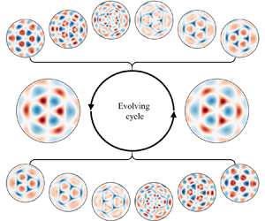
 $0.04\, \mathrm {s}$ is observed, which may be due to phase differences among the wave components involved. Our focus is on the transitional processes between the two most deformed patterns in a wave period. Two groups of small-elevation cases, each including six successive phases (indicated by the boxes in figure 8c), are selected to reconstruct the evolving surface patterns for each half-cycle, as shown in figure 8(d,e). Obviously, similar
 ${\rm \pi} /3$ rotations hold for these transitional cases. Some remarkable localized structures were also observed in the small-elevation periods when harmonics dominated the surface disturbance. Such wave components evolve according to their inherent cycles and may be examined within their high-expressed phases. It is therefore useful to study the dynamic behaviour of these intricate interfacial structures within the small-elevation phases of subharmonic components (
 $\eta (P_0)\approx 0$). By tracing the wave crests (red coloured in figure 8a,b), the surface peaks collapse into several small waves travelling along the radius or rings and localized wave interactions occur after a short while. As a result, a
 ${\rm \pi} /3$ rotation of the overall pattern occurs after half a wave period. Meanwhile, the processes of collapse and interaction are seemingly time asymmetric due to nonlinear motions of the thin liquid layer. Later on, we focus on modal decomposition by conducting profile analysis of this investigated mode.
Cyclic evolution of surface structures of the full-response  $(3,3)$ mode at final steady states. The two largest-elevation patterns are shown in (a,b), and the periodic variation in localized surface elevation at the peak point
 $P_0$ is given in (c). To indicate transitions between pattern (a) and pattern (b), six solid-boxed cases and six dashed-boxed cases in small-elevation phases are selected, and the reconstructed patterns of these cases are sequentially displayed in (d,e), respectively. Experimental parameters include
 $\xi =0.15\, \mathrm {mm}$ and
 $\varOmega _0/2{\rm \pi} =18.5\, \mathrm {Hz}$. The wave period
 $T_F$ is invariably equal to
 $4{\rm \pi} /\varOmega _0$. A common colour bar is given for all patterns, where
 $|\eta |_{max}$ denotes the maximal modulus of surface elevation in each pattern. The complete pattern evolution of this investigated mode over a wave period can be seen in the supplementary animation available at https://doi.org/10.1017/jfm.2023.838.

Before continuing our analysis of the investigated surface dynamics, it is necessary to introduce the coordinate systems as shown in figure 9(a). At first, the information of refracted images is stored in the plane Cartesian coordinate system  $O^{\prime }\text {-} x^{\prime }y^{\prime }$, and a unidirectional reversed transformation to another plane coordinate system
 $O^{\prime \prime }\text {-} x^{\prime \prime }y^{\prime \prime }$ is carried out as part of the AL-DIC procedure. Then, the reconstructed surface is obtained in the corresponding Cartesian coordinate system
 $O^{\prime \prime }\text {-} x^{\prime \prime }y^{\prime \prime }z^{\prime \prime }$. To facilitate subsequent analysis, a cylindrical coordinate system is utilised to eliminate the azimuthal phase difference
 $\theta _0$ between experimental and target images as identified in figure 9(b). The system origin is located at the centre of the stationary circular fluid interface, with the polar line
 $\theta =0$ passing through the projection
 $P_0$ of the standing wave crest point on the horizontal plane
 $z=0$. Here, instantaneous surface deformation is denoted by the expression for
 $\eta (r,\theta,t)$, where
 $r$ is the dimensionless length scaled by
 $R$. Please note that previous figures are presented in the Cartesian coordinate system
 $O^{\prime \prime }\text {-} x^{\prime \prime }y^{\prime \prime }z^{\prime \prime }$ whereas the following reconstructed views of the wave interface are based on the cylindrical coordinate system shown in figure 9.
(a) Coordinate transformations and cylindrical geometry for Faraday waves in a cylindrical container. (b) Multi-dimensional views of mode  $(3,3)$ and definition of the azimuthal phase difference
 $\theta _0$.

As derived by Benjamin & Ursell (Reference Benjamin and Ursell1954), the modal structure of  $\nu$-fold Faraday waves with a free contact line can be expanded as a series of eigenmodes, which are typically sought in the form of
 $\cos (\nu \theta )\,\mathrm {J}_\nu (k_{\nu,n} r)$, where the eigennumber
 $k_{\nu,n}$ is the
 $n$th root of
 $\mathrm {J}_\nu ^\prime$. Similarly, Kidambi (Reference Kidambi2013) proposed a spatial scheme,
 $\cos (\nu \theta )\,\mathrm {J}_\nu (\delta _{\nu,n} r)$ with
 $\delta _{\nu,n}$ the
 $n$th root of
 $\mathrm {J}_\nu$, to describe Faraday waves in a brimful cylinder where the contact line was pinned. Owing to the decoupling of
 $\theta$ and
 $r$, azimuthal structures and radial profiles correspond to cosine functions and Bessel functions, respectively. However, the foregoing simple expression is unable to adequately explain the localized structures observed in the small-elevation cases shown in figure 8(d,e). A more intricate expression for harmonics is required to capture these structures. We start by examining the variation of radial profiles at
 $\theta =0$ in figure 10(a). Two typical profiles at the large-elevation phase
 $0.46T_F$ and the small-elevation phase
 $0.74T_F$ are presented in the bottom subfigure. Note that the azimuthal profiles at two phases with the same value are also characterized in figure 10(b–f) for various radial cases. In figure 10(a) three radial regions of peaks or troughs (distinguished as inner, middle and outer regions) are identified according to the Bessel function
 $\mathrm {J}_3(\delta _{3,3} r)$ with the two separating lines located at
 $r\approx 0.5$ and
 $r\approx 0.85$, indicated by solid lines and labelled ‘(b)’ and ‘(c)’, respectively. Meanwhile, two small-elevation periods between the peaks and troughs correspond to the transitions over two half-cycles. As indicated by arrows, the middle peaks collapse into two localized contra-travelling waves in radial directions, while the inner and outer peaks each form a single radial travelling wave. This generation of radial travelling waves is attributed to the radial surface profiles of harmonics, which may possess five radial nodes as identified from the radial profile at
 $0.74T_F$. Furthermore, the temporal variations of the two separating lines are displayed in figure 10(b,c), respectively. In both cases, the magnitudes of
 $\mathrm {J}_3(\delta _{3,3} r)$ are relatively small, allowing circumferential structures with six and nine high points to be captured at certain phases, as evident in the corresponding subfigures at the bottom. This implies that the harmonics are six-fold, nine-fold and even higher
 $3m$-fold (
 $m> 3$). Additionally, figure 10(d–f) illustrates the temporal evolution of circumferential slice structures across the inner, middle and outer peaks, respectively, which are indicated by dashed lines with labels ‘(d)’, ‘(e)’ and ‘( f)’ in figure 10(a). Transitions from peaks to troughs are observed in the three cases (d–f) where subharmonic components dominate. In the inner and middle cases, each peak evolves into two localized contra-travelling waves in circumferential directions as marked by arrows in figure 10(d,e), causing six nodes to develop on the circles during these small-elevation phases as evident in the profiles at
 $0.74T_F$ displayed in the two corresponding subfigures. For the outer slice in figure 10( f), similar spatiotemporal characteristics related to travelling waves may be discerned (indicated by the arrows). Nine azimuthal peaks occur in both the large-elevation phase and the small-elevation phase (as seen in the subfigure). This indicates the presence of another subharmonic wave component with nine-fold symmetry. Additionally, we can deduce that the structure of this high-order component has
 $\cos {9\theta }\,\mathrm {J}_{9}(\delta _{9,1}r)$ form, noting the presence of nine-fold symmetry in figure 10(c) and its absence in figure 10(b,d,e).
Localized evolution of circumferential and radial surface profiles for  $(3,3)$ mode. Profile elevation magnitudes are obtained by 3-D interpolation of reconstructions. For each radial and circumferential profile, the spatiotemporal variation beyond a wave period and typical structures at two phases, one large elevation (
 $0.46T_F$) and the other small elevation (
 $0.74T_F$), are displayed. The variation of slice structures at
 $\theta =0$ is depicted in (a) where arrows indicate localized travelling waves in the radial direction. Three dominant regions of peaks or troughs occur in the radial direction and are defined as inner, middle and outer regions. Two solid lines,
 $r=0.5\ \text {and}\ 0.85$, labelled ‘(b)’ and ‘(c)’, roughly separate the three radial regions. The three dashed lines,
 $r=0.357,0.668\ \text {and}\ 0.925$, labelled ‘(d)’, ‘(e)’ and ‘( f)’, pass through three peaks in the radial direction. Steady-state evolution processes of circumferential slices across five of the indicated lines are displayed in (b–f). Arrows in (d–f) indicate the localized travelling waves in circumferential directions. The colour bars refer to surface elevations in units of
 $\mathrm {mm}$.

The foregoing analysis indicates that the surface structure of symmetric Faraday waves in our experiments may be represented by the multi-azimuth expressions as follows. For any given  $r$, the azimuthal structure of mode
 $(\nu,\zeta )$ is
 $\nu$-fold overall, and localized symmetries of multiple azimuthal numbers, called multi-azimuth structures, may be observed during certain phases, especially those related to small-elevation components. Hence, the azimuthal structures of the wave components of interest can be approximated by cosine functions
 $\cos (m\nu \theta )\ (m=1,2,3,\ldots )$ and the radial structures fitted by Bessel functions
 $\mathrm {J}_{m \nu }(\delta _{m\nu,n} r)\ (n=1,2,3,\ldots )$. Furthermore, resonant surface waves
 $(\nu,\zeta )$ in a brimful cylinder can be regarded as the superposition of unstable eigenmodes expressed as functions of
 $\cos (m\nu \theta )\,\mathrm {J}_{m\nu }(\delta _{m\nu,n} r)$. Defining these eigenmodes as
 $\nu$-basis modes
 $(m,n)_\nu$, we obtain
 \begin{equation} (\nu,\zeta) = \sum_{m=1}^{\infty}\sum_{n=1}^{\infty}(m,n)_\nu, \end{equation}
where  $m$ denotes the azimuthal multiplier and
 $n$ denotes the radial multiplier. The
 $\nu$-basis modes
 $(1,n)_\nu$ are different from the eigenmodes proposed by Benjamin & Ursell (Reference Benjamin and Ursell1954) due to the pinned boundary condition in our experiments. It is straightforward to infer that in the investigated
 $(3,3)$ mode, the subharmonic
 $(1,3)_3$ component dominates and its harmonics are mostly composed of
 $(m,{\cdot })_3$ modes with
 $m\geq 2$. The foregoing analysis of the outer slice also implies that another possible subharmonic component may relate to the
 $(3,1)_3$ mode. We speculate that the
 $(1,2)_3$ mode may also have a large magnitude given that the outer region is rather narrow, owing to the node restriction on the pinned boundary (
 $\eta |_{r=1}=0$).
4. Modal decomposition
Standing waves excited much above onset are not inherently pure, due to the presence of harmonics with multi-azimuth structures, which do not align properly with the eigenmodes derived by Benjamin & Ursell (Reference Benjamin and Ursell1954) and Kidambi (Reference Kidambi2013). These standing waves, which are not competitive modes, result from the superposition of various unstable modes. Using the FS-SS method, we have obtained highly accurate, full 3-D spatial reconstructions of Faraday waves in a cylindrical domain, which have enabled us to quantitatively detect the fast pattern evolution and achieve modal decomposition of the superposed standing waves in full-response cases.
4.1. Spatiotemporal surface fitting
We hypothesise that the surface function of a certain mode  $(\nu,\zeta )$ excited above the Faraday threshold may be approximated by a series of
 $\nu$-basis modes
 $(m,n)_\nu$ (3.1), such that the spatial decomposition is given by
 \begin{equation} \eta(r,\theta,t)=\sum_{m=1}^{M}\sum_{n=1}^{N}a_{m,n}(t) \cos{m\nu\theta} \,\mathrm{J}_{m\nu}(\delta_{m\nu,n}r), \end{equation}
where the total modal number  $MN$ is determined by the calculated limits
 $M$ and
 $N$ of two multipliers
 $m$ and
 $n$, respectively. Normally,
 $N$ is set to an integer value much greater than
 $\zeta$ in order to obtain a more accurate expression for radial structures in the deformed surface. Additionally, an adequately large value of
 $M$ (
 $M\geq 2$) should be identified because of the existence of circumferential structures with multiple azimuths, particularly for small local features that occur during the transition period. We commence by fitting the reconstructed surface, generated by the FS-SS method, with a multi-mode function (4.1) and then analyse the modal information by examining the fitted coefficients
 $a_{m,n}$. For example, we evaluate the observed mode
 $(3,3)$ in figure 8 to indicate the accuracy of the 3-basis modal expression (4.1) using the spatial surface-fitting procedure.
We establish a corresponding equation for every grid point in the circular domain to generate a linear system containing  $Q$ equations and then solve this over-determined problem with
 $MN$ unknowns. A similar method ‘
 $\backslash$’, which has been employed in the calculation of the inverse gradient field, is performed to acquire the least-squares solution of the fitted surface. We set
 $M=6$ and
 $N=15$ (a total of 90
 $\nu$-basis modes) to obtain surface-fitting results for the investigated modes
 $(3,3)$. It can be seen in figure 11 that the spatial expression in the form of (4.1) provides a satisfactory fit to the reconstructed surface despite the small, complicated displacement of the modal transition. For other explored modes, the results of spatial fitting with
 $\nu$-basis expressions are found to be qualitatively of high accuracy, confirming that resonant modes
 $(\nu,\zeta )$ excited above the Faraday threshold can be linearly decomposed into corresponding
 $\nu$-basis modes
 $(m,n)_\nu$.
Comparison between (a) reconstructed patterns (see figure 8e) and (b) fitted patterns using 3-basis modal expressions. A common colour bar is given for all patterns where  $|\eta |_{max}$ denotes the maximal modulus of surface elevation calculated from the reconstructions of each pattern in the first row (a). The close agreement demonstrates the validity of the spatial surface-fitting scheme used herein. Complete surface-fitting patterns over a wave period can be seen in the supplementary animation.

We now examine the spatiotemporal characteristics of the  $\nu$-basis modes and perform further analysis on the time-varying coefficients
 $a_{m,n}(t)$ to reveal the magnitude and periodicity of
 $(m,n)_\nu$. Many
 $\nu$-basis modes are applied in the surface-fitting computation, and intuitive speculation concerning the dominant modes of the observed
 $(\nu,\zeta )$ mode suggests that the largest two are
 $(1,\zeta )_\nu$ and
 $(1,\zeta -1)_\nu$ due to constraint by the cylindrical boundary on the spatial structures of
 $(\nu,\zeta )$. Furthermore, it is useful to discern other relatively dominant wave components in such mode superposition, and so we conduct a comparative analysis of the
 $a_{m,n}(t)$ coefficients. Figure 12 displays the magnitude
 $\gamma _{m,n}$ plots of
 $\nu$-basis modes for three investigated modes, where
 $\gamma _{m,n}$ denotes the amplitude of time varying
 $a_{m,n}(t)$,
 \begin{equation} \gamma_{m,n}=\max_t{\left|a_{m,n}(t)\right|}. \end{equation}
The magnitude of  $\gamma _{m,n}$ determines the amplitude of the
 $\nu$-basis mode
 $(m,n)_\nu$ for a given experimental mode
 $(\nu,\zeta )$, which also demonstrates the corresponding degree of dominance of the
 $\nu$-basis mode. In figure 12 the discrete scattered curves of magnitude
 $\gamma _{m,n}$ for different
 $m$ contain multiple peaks, which allow us to deduce the dominant modes. These
 $\nu$-basis modes at peaks associated with each
 $m$ are referred to as peak modes. The magnitudes
 $\gamma _{1,\zeta }$ and
 $\gamma _{1,\zeta -1}$ are found to be substantially greater than the other coefficients, in accordance with our earlier hypothesis. We suggest that the non-peak modes modulate the radial structures (wavenumbers) of peak modes to satisfy the dispersion relation. For this reason, our paper focuses solely on these peak modes, which are related to surface instability or wave interactions.
Magnitudes  $\gamma _{m,n}$ of fitting coefficients
 $a_{m,n}$ for three experimental modes (a–c) with indicated different vibration driving parameters displayed as a function of azimuthal multiplier
 $m$ and radial multiplier
 $n$. Major peaks are labelled according to the dominant
 $(m,n)_\nu$ modes. Magnitudes
 $\gamma _{m,n}$ associated with given
 $m$ are indicated by the coloured bands. Results are shown for (a)
 $(2,3)$
 $\xi = 0.2$ mm,
 $\varOmega _0/2{\rm \pi} = 15.5$ Hz; (b)
 $(4,2)$
 $\xi = 0.175$ mm,
 $\varOmega _0/2{\rm \pi} = 15.2$ Hz; (c)
 $(3,3)$
 $\xi = 0.15$ mm,
 $\varOmega _0/2{\rm \pi} = 18.5$ Hz.

For a given  $\nu$-basis mode with
 $m$ and
 $n$ non-equivalent to any of the peak modes, the magnitude
 $\gamma _{m,n}$ is negligible, suggesting that wave energy is primarily stored in peak modes. Hence, the spatial structures of the explored mode
 $(\nu,\zeta )$ mainly depend on those of peak modes, and a larger number of peak modes leads to a more deformed modal pattern throughout the wave period. Apart from the peak modes, the magnitudes of the
 $\nu$-basis modes
 $(m,n)_\nu$ rapidly reduce with progressively larger
 $m$ and
 $n$. Moreover,
 $\gamma _{m,n}$ disappears when
 $m$ and
 $n$ reach critical integer values, implying weak or no excitation of the corresponding modes in the experiments. As a result, the upper limits of
 $m$ and
 $n$ can be ascertained in order to obtain a sufficiently precise fitting surface. However, not all peak modes can be regarded as dominant modes triggered by surface instability, which should be further classified according to frequency distribution, and so a detailed analysis follows concerning the temporal fitting results for
 $a_{m,n}(t)$.
We consider several peak modes with  $m\leq 3$ for three cases of interest, which are labelled
 $(m,n)_\nu$ in figure 12. Further analysis evaluates the periodicity relation for these peak modes, based on frequency decomposition of the time varying
 $a_{m,n}(t)$. The observed Faraday modes are subharmonic resonance, excited at frequency
 $\omega _0$ equal to half the driving angular frequency such that
 $\omega _0=\varOmega _0 / 2$. The temporal decomposition is expressed as the following sum of multi-frequency cosine functions:
 \begin{equation} a_{m,n}(t) = \sum_{l=0}^{\infty} \chi_l \cos{l \omega_0 t}. \end{equation}
Here the fitting coefficients  $\chi _l$ are different for various
 $a_{m,n}(t)$. Due to the temporal difference between the selected frames and expression (4.3), we adopt a more general form to fit the time-varying coefficient
 $a_{m,n}(t)$ in practical calculations, which reads as
 \begin{equation} a_{m,n}(t) = \sum_{l=0}^{\infty} \chi_l \cos{l \omega_0 t}+\sum_{l=1}^{\infty} \hat{\chi}_l \sin{l \omega_0 t}, \end{equation}
where  $\hat {\chi }_l$ are coefficients corresponding to the additional sine terms
 ${\sin {l \omega _0 t}}$ (
 ${l=1,2,3,\ldots}$) in the expansion. For computational purposes, the upper limit of
 $l$ is truncated to
 $L$.
We now let  $L=10$, and perform linear fitting using the Matlab function lsqcurvefit() of the approximate expression (4.4) to discrete
 $a_{m,n}(t)$ values for the three experimental modes. Figure 13(a,c,e) shows the fitting results of indicated dominant modes over an evolving period
 $T_F$ (
 $=2{\rm \pi} /\omega _0$). It can be seen that the fitted curves of
 $a_{m,n}(t)$ are in relatively close agreement with the calculated evolution. Close-fit results are also obtained for the remaining modes in figure 12, confirming that (4.4) (or (4.3)) precisely replicates the periodicity of
 $\nu$-basis modes
 $(m,n)_\nu$. We then focus on the fitting coefficients
 $\chi _l$ and
 $\widehat {\chi _l}$. The right pseudo-colour illustrations in figure 13 show the normalized magnitudes
 $\hat {\gamma }_{m,n,l}$ of frequency components for the indicated modes
 $(m,n)_\nu$, each of which is defined as
 \begin{equation} \hat{\gamma}_{m,n,l}=\left\{ \begin{array}{@{}ll@{}} \displaystyle\dfrac{\left|\chi_0\right|}{\gamma_{m,n}}, & l=0, \\ \displaystyle\dfrac{\sqrt{\chi_l^2+\hat{\chi}_l^2}}{\gamma_{m,n}}, & l>0, \end{array} \right. \end{equation}
where  $\chi _0$,
 $\chi _l$ and
 $\hat {\chi }_l$ (
 $l=1,2,\ldots,L$) are the fitting coefficients of
 $a_{m,n}$. For simplicity, we define the component with angular frequency
 $l\omega _0$ of
 $a_{m,n}(t)$ as the corresponding
 $l\omega _0$ component of the
 $\nu$-basis mode
 $(m,n)_\nu$, and peak modes with dominant
 $l\omega _0$ component as
 $l\omega _0$-dominant modes. As shown in figure 13(b,d, f), the
 $\omega _0$ and
 $2\omega _0$ components dominate, so these modes are purely subharmonic or harmonic. The most dominant
 $(1,\zeta )_\nu$ modes of the three different
 $(\nu,\zeta )$ modes oscillate at an angular frequency
 $\omega _0$. The dominant components of peak modes
 $(2,5)_2$,
 $(2,5)_3$ and
 $(2,3)_4$ are
 $2\omega _0$ components. On this basis, peak modes with dominant
 $\omega _0$ or
 $2\omega _0$ components are denoted as dominant modes, with
 $(1,\zeta )_\nu ^{sh}$ invariably the most dominant mode in the modal decomposition of
 $(\nu,\zeta )$. For these
 $\nu$-basis modes
 $(m,n)_\nu$ with constant
 $m$, no more than two dominant modes usually exist, and one is subharmonic and the other is harmonic if two dominant modes emerge with the same
 $m$, such as
 $(2,5)^{sh}$ and
 $(2,2)^{h}$ in figure 13(a,b). Meanwhile, the subharmonic dominant mode
 $(3,1)_3$ is indeed observed, as inferred in the discussion for figure 10.
Temporal fitting of dominant modes for three experimental cases of Faraday waves: plots (a,c,e) show the resulting  $a_{m,n}(t)$ time series; and (b,d, f) pseudo-colour diagrams, where
 $\omega /\omega _0$ equals
 $l$, show the normalized magnitude
 $\hat {\gamma }_{m,n,l}$ of multiple frequency components, demonstrating the frequency distribution of selected dominant
 $\nu$-basis modes
 $(m,n)_\nu$. Deeper-coloured blocks with larger
 $\hat {\gamma }_{m,n,l}$ represent dominant frequency components of given dominant modes. Results are shown for (a,b)
 $(2,3)$
 $\xi = 0.2$ mm,
 $\varOmega _0/2{\rm \pi} = 15.5$ Hz; (c,d)
 $(4,2)$
 $\xi = 0.175$ mm,
 $\varOmega _0/2{\rm \pi} = 15.2$ Hz; (e, f)
 $(3,3)$
 $\xi = 0.15$ mm,
 $\varOmega _0/2{\rm \pi} = 18.5$ Hz.

4.2. Peak modes
It is significant to focus on the spatiotemporal characteristics of peak modes because they strongly correlate with multi-azimuth structures appearing in the fast wave evolution. The pseudo-colour illustrations in figure 14(a–c) depict the logarithmic magnitude  $\log _{10}{\gamma _{m,n}}$ of
 $MN$
 $\nu$-basis modes in a
 $m$–
 $n$ plane for three investigated cases. Deeper red blocks marked with circles represent peak modes of relatively large magnitude in figure 12; these dominant modes are marked by blue pentagrams. In the
 $m$–
 $n$ plane we observe that the peak modes appear to be regulated in a seemingly uniform arrangement within a constrained range of
 $m$ and
 $n$ values. We connect these peak modes with solid lines and dashed lines in two directions in figure 14(a–c). For simplicity, we heuristically refer to the sequences of uniformly arranged peak modes on solid lines and dashed lines as peak chains and frequency levels, respectively.
Pseudo-colour diagrams that indicate the magnitude  $\log _{10}{\gamma _{m,n}}$ of the
 $\nu$-basis modes for three investigated modes (a–c), with corresponding peak modes in figure 12 marked by hollow circles. These dominant modes are also marked by blue pentagrams. Peak modes are uniformly arranged in the
 $m$–
 $n$ plane and connected by solid lines and dashed lines in two directions, which refer to peak chains and frequency levels, respectively. Four peak chains of mode
 $(3,3)$ are identified in (d). The pseudo-colour illustrations of
 $\hat {\gamma }_{m,n,l}$ demonstrate the frequency distribution of peak modes
 $(m,n)_\nu$ on a certain peak chain (e) and four specific frequency levels. Colour scales for
 $\log _{10}{\gamma _{m,n}}$ and
 $\hat {\gamma }_{m,n,l}$ are given on the right. Results are shown for (a)
 $(2,3)$
 $\xi = 0.2$ mm,
 $\varOmega _0/2{\rm \pi} = 15.5$ Hz; (b)
 $(4,2)$
 $\xi = 0.175$ mm,
 $\varOmega _0/2{\rm \pi} = 15.2$ Hz; (c)
 $(3,3)$
 $\xi = 0.15$ mm,
 $\varOmega _0/2{\rm \pi} = 18.5$ Hz; (e)
 $(1,3)_3 \to (2,5)_3 \to (3,7)_3 \to (4,9)_3$.

The peak chains starting at  $(1,\zeta )_\nu$ for modes
 $(2,3)$,
 $(3,3)$ and
 $(4,2)$ are given by
 \begin{equation} \left. \begin{aligned} (1,3)_2 & \rightarrow (2,5)_2 \rightarrow (3,7)_2 \rightarrow (4,9)_2 \rightarrow \cdots, \\ (1,3)_3 & \rightarrow (2,5)_3 \rightarrow (3,7)_3 \rightarrow (4,9)_3 \rightarrow \cdots, \\ (1,2)_4 & \rightarrow (2,3)_4 \rightarrow (3,4)_4 \rightarrow (4,5)_4 \rightarrow (5,6)_4 \rightarrow \cdots, \end{aligned} \right\} \end{equation}
where the right arrows specify the primary transmission direction of energy and spatiotemporal information as discussed in the following sections. Interestingly, the indices  $m$ and
 $n$ of a particular peak chain are in the order of an arithmetic progression, i.e. the next peak mode after
 $(m,n)_\nu$ is always
 $(m+1,n+2)_\nu$ for modes
 $(2,3)$ and
 $(3,3)$, whereas that for
 $(4,2)$ is
 $(m+1,n+1)_\nu$, which is related to the first two peak modes in any given peak chain. Hence, we suggest that the uniform arrangement of peak modes is arithmetic-progression-like. Moreover, more than one uniformly arranged peak chain can be discerned for any arbitrary
 $(\nu,\zeta )$ mode. For example, four peak chains for the
 $(3,3)$ mode are indicated in figure 14(d), where the peak modes are arranged according to the solid lines and dashed lines in figure 14(c). A similar analysis is next carried out for the frequency characteristics of peak modes on solid lines (peak chains) and dashed lines (frequency levels) for
 $(3,3)$. As shown in figure 14(e), the frequency distribution for these modes in a certain peak chain demonstrates that the dominant frequency components
 $l\omega _0$ (deep blocks) are uniformly arranged with increasing
 $l$ along the peak chains, which is also arithmetic-progression-like. For example, the
 $l$th mode in the peak chains starting at
 $(1,\zeta )_\nu$ is
 $l\omega _0$ dominant. A more universal rule is that a mode in a certain chain is
 $l\omega _0$ dominant whereas the next mode is
 $(l+1)\omega _0$ dominant. Figure 14( f) shows the frequency distribution of these peak modes at four frequency levels. One can observe that those modes at the same frequency level possess the same dominant frequency (
 $l\omega _0$) provided that the frequency levels are sorted in a
 $1,2,\ldots,l,\ldots$ sequence corresponding to the increasing dominant frequency of modes along the peak chain. White blocks represent a lack of corresponding frequency components in the peak modes, whose uniform arrangements in figure 14(e, f) reveal that these peak modes on peak chains and frequency levels are either subharmonic (only odd
 $l$) or harmonic (only even
 $l$). However, an exception exists for
 $(2,2)$ whereby
 $(2,2)_2$ and
 $(2,5)_2$ have impure frequency distributions, as evident in figure 13(a,b), due to co-interference. This invariably occurs when two dominant modes occur with the same azimuthal structures excited by surface instability.
Hence, according to the frequency distributions, we define the modal decomposition of  $(\nu,\zeta )$ by
 \begin{equation} (\nu,\zeta) = \sum_{n=1}^{\infty}\sum_{m=1}^{\infty}\left[ (m,n)_\nu^{sh} + (m,n)_\nu^{h}\right], \end{equation}
where the quantities  $m$,
 $n$ and
 $\nu$ indicate spatial characteristics, and the superscripts
 $sh$ and
 $h$ represent temporal characteristics. Accordingly, the temporal expression (4.3) is rewritten as the following combination of subharmonic and harmonic components:
 \begin{equation} a_{m,n}(t) = \underbrace{\sum_{l=0}^{\infty} \chi_l^n \cos{2 l \omega_0 t}}_{\text{harmonic}}+\underbrace{\sum_{l=0}^{\infty} \hat{\chi}_l^n \cos{(2 l+1)\omega_0 t}}_{\text{subharmonic}}. \end{equation}
4.3. Modal interaction with energy transfer
We next pay attention to the mechanism of arithmetic-progression-like arrangements of peak modes in the  $m$–
 $n$ plane (see figure 14a–c) and their frequency distributions (see figure 14e, f). We recall that the spatiotemporal decomposition of mode
 $(\nu,\zeta )$ is in the form of
 $\nu$-basis modes
 $(m,n)_\nu$, and the minimum spatiotemporal component of
 $(m,n)_\nu$ is expressed as
 $\cos {l\omega _0 t}\cos {m\nu \theta }\,\mathrm {J}_{m\nu }(\delta _{m\nu,n}r)$. To describe the generation of the arithmetic combination of mode indices, we provide a qualitative derivation based on the simple multiplication of two minimum spatiotemporal components, which represents the interaction of the
 $l_1\omega _0$ component of mode
 $(m_1,n_1)_\nu$ and
 $l_2\omega _0$ component of mode
 $(m_2,n_2)_\nu$,
 $$\begin{gather} \cos{l_1 \omega_0
t}\cos{m_1 \nu
\theta}\,\mathrm{J}_{m_1\nu}(\delta_{m_1\nu,n_1}r)\,
\cos{l_2 \omega_0 t}\cos{m_2 \nu
\theta}\,\mathrm{J}_{m_2\nu}(\delta_{m_2\nu,n_2}r)
\nonumber\\ = \underbrace{\cos{m_1 \nu \theta}\cos{m_2 \nu
\theta}\,\mathrm{J}_{m_1\nu}(\delta_{m_1\nu,n_1}r)
\mathrm{J}_{m_2\nu}(\delta_{m_2\nu,n_2}r)}_{\text{(I)}}
\,\underbrace{\cos{l_1 \omega_0 t}
\cos{l_2 \omega_0 t}}_{\text{(II)}},
\end{gather}$$
where  $m_1$,
 $m_2$,
 $n_1$,
 $n_2$,
 $l_1$ and
 $l_2$ are positive integers; and terms (I) and (II) are spatially and temporally related products. Self-interaction is approximated by the overall operation (4.9) with
 $m_1=m_2$,
 $n_1=n_2$ and
 $l_1=l_2$. Due to the pinned boundary condition, the zero points of the two Bessel functions in term (I) at
 $r=1$ are coincident, and so the number of nodes of the Bessel function product in the radial interval (
 $0< r\leq 1$) is
 $n_1+n_2-1$. Moreover, the azimuthal terms
 $\cos {(m_1-m_2)\nu \theta }$ and
 $\cos {(m_1+m_2) \nu \theta }$ are derived from the multiplication of two cosine functions. Hence, we obtain a criterion that the interaction of
 $(m_1,n_1)_\nu$ and
 $(m_2,n_2)_\nu$, which both lie on a certain peak chain, is necessary for a new mode
 $(m_1+m_2,n_1+n_2-1)_\nu$ to be created belonging to the same peak chain. It can be verified that peak chains in figure 14(a–c) satisfy this criterion, and thus, the rule of arithmetic-progression-like arrangement of peak modes in the
 $m$–
 $n$ plane follows accordingly. Similarly, for term (II), two frequency components
 $\cos {|l_1-l_2| \omega _0 t}$ and
 $\cos {|l_1+l_2| \omega _0 t}$ are generated from the interaction between the
 $l_1\omega _0$ component and
 $l_2\omega _0$ component. The dominant frequency of these peak modes along the peak chain (4.6) also increases progressively as shown in figure 14(e), and is consistent with the simple nonlinear interaction of modes on peak chains. Here, using the simple multiplication (4.9), we provide typical examples about
 $(4,9)_3$ to display mode interaction on peak chains. The generation of
 $(4,9)_3$ originates from (a) the interaction of
 $(1,3)_3$ and
 $(3,7)_3$ and (b) the self-interaction of
 $(2,5)_3$, which both induce three frequency components (
 $0$,
 $2\omega _0$ and
 $4\omega _0$) as evident in figure 14(e). Self-interaction is usually a relatively weak process in wave interaction. Similar nonlinear interactions appear between arbitrary, two or more, peak modes, and so other peak modes of larger
 $m$ and
 $n$ with specific frequency distributions in peak chains emerge accordingly, which result in the uniform arrangements of peak modes and dominant frequency components displayed in figure 14. Note that peak chains (4.6) labelled with right-directed arrows indicate that the two preceding modes can (self-)interact to generate a third mode, which we refer to as resonance involving three standing modes. Although nonlinear wave interactions in the present experimental system are far more complex than represented by simple multiplication (4.9), such schemes nevertheless enable us to understand the spatiotemporal structures of harmonics induced by wave interaction.
Furthermore, although the aforementioned results are derived from the surface fitting of symmetric Faraday waves at the final steady state in experiments where the driving parameters much exceed the instability threshold, the chain-like dynamics of superposed standing wave components, identified as  $\nu$-basis modes, enable us to backtrack the pattern formation. Rajchenbach et al. (Reference Rajchenbach, Clamond and Leroux2013) suggested a mechanism based on three-wave resonance to explain the triggering of parametrically forced surface waves with certain symmetries that were observed in the experiments. However, such a nonlinear mechanism can only describe the initial response and does not account for the presence of high-order harmonics in the final periodic state. Using modal decomposition, we gain insight into the mechanism that enhances symmetries triggered during the initial response period as they evolve to reach steady states. Here, analogous resonant coupling between three standing waves is used to describe the observed spatiotemporal characteristics of high-order harmonics, as introduced in (4.9). The interaction between two primary modes,
 $(m_1,n_1)_\nu$ and
 $(m_2,n_2)_\nu$, can result in the emergence of a secondary mode
 $(m_1+m_2,n_1+n_2-1)_\nu$, allowing for continuous energy supply. By extending the mechanism in Rajchenbach et al. (Reference Rajchenbach, Clamond and Leroux2013) and incorporating nonlinear wave interactions, we provide a comprehensive explanation of overall pattern formation in our experiments. At first, using energy supplied from the forcing vibration of the shaker, surface instability is triggered resulting in the emergence of dominant modes, which are either subharmonic (
 $\omega _0$ dominant) or harmonic (
 $2\omega _0$ dominant). Their symmetries are selected by the contact angle between two waves involved in three-wave resonance. Once these dominant modes are established, they become locked and subsequently grow. Persistent nonlinear wave interactions, including self-interactions, take place with sustained energy transfer, and peak chains and frequency levels with specific spatiotemporal characteristics are then uniquely determined. Consequently, newly formed wave components with complex spatiotemporal structures originate from the coupled interaction of several dominant waves and simultaneously extract a small amount of energy. After a certain number of forcing cycles, the pattern evolution process becomes steady, and a balance is achieved among energy supply, transfer and dissipation. In this way, energy transfer in each investigated wave
 $(\nu,\zeta )$ primarily occurs along the peak chain (4.6), and the arithmetic-progression-like arrangement is determined by dominant modes and wave interactions. Hence, the wave components involved can be classified as being of two types: dominant modes determined by the effect of parametric instability at the air–liquid interface; and harmonics induced by wave interactions. The generation of dominant modes is still not fully understood, and therefore, it is crucial to provide theoretical verification regarding the selection of these dominant modes.
5. Theoretical verification
We recall that Faraday wave response of single symmetry involves the superposition of a few eigenmodes with certain wavelengths selected in a small system. Linear stability analysis of such a system using appropriate modal solutions (eigenmodes) in inviscid governing equations has been undertaken to predict the instability threshold for cases of the free contact-line condition Benjamin & Ursell (Reference Benjamin and Ursell1954) and pinned contact-line condition (Kidambi Reference Kidambi2013). The accuracy of these theoretical predictions depended on the selection of modal solutions, the treatment of viscous damping and the contact-line condition. A recent study by Bongarzone et al. (Reference Bongarzone, Viola, Camarri and Gallaire2022) carefully incorporated these factors in a weakly nonlinear analysis. Note that investigated modes observed above the instability threshold can be regarded as the response that is composed of purely subharmonic modes near onset caused by strong nonlinearity, primarily determined by the control distance. We assume that these dominant modes naturally emerge as the selected response due to surface instability. Based on the definition of eigenmodes ( $\nu$-basis modes), we now introduce a linear stability analysis, inspired by Kidambi (Reference Kidambi2013), to verify the existence of the aforementioned dominant modes.
5.1. Theory of inviscid Faraday waves in a brimful cylinder
Consider the vertical forced oscillation of liquid in a brimful cylindrical container of radius  $R$ and height
 $H$ shown in figure 9(b). The container is filled to the brim with a low-viscosity liquid (i.e. water) of density
 $\rho$ and surface tension
 $\sigma$ such that the contact line of the liquid surface and the lateral wall remains pinned during the course of continuous oscillation. Surface patterns and interface deformation
 $\eta (r,\theta,t)$, restored by gravity
 $g$ and surface tension
 $\sigma$, are generated under the parametric driving force expressed by dimensionless acceleration amplitude
 $\epsilon$ and dimensionless angular frequency
 $\varOmega$. Here, linear spatial dimensions are scaled by
 $R$, time by
 $\sqrt {\rho R^3/\sigma }$, velocity potential by
 $\sqrt {\sigma R/\rho }$ and acceleration by
 $g$. Dimensionless governing equations are used in the linear stability analysis of the free-surface disturbance. Assuming the liquid is inviscid and irrotational, the velocity potential
 $\phi$ satisfies Laplace's equation
 \begin{equation} \nabla^2 \phi=0. \end{equation}
No-penetration conditions at the bottom and lateral walls of the container are given by
 \begin{equation} \left.\frac{\partial \phi}{\partial z}\right|_{z={-}h}=0,\quad \left.\frac{\partial \phi}{\partial r}\right|_{r=1}=0, \end{equation}
where dimensionless height  $h=H/R$.
At the free surface, assumed to be at  $z=0$, the kinematic condition,
 \begin{equation} \frac{\partial \phi}{\partial z}=\frac{\partial \eta}{\partial t}, \end{equation}
and the dynamic condition,
 \begin{equation} \frac{\partial\phi}{\partial t}+Bo(1-\epsilon\cos{\varOmega t})\eta-\left(\frac{\partial^2\eta}{\partial r^2}+\frac{1}{r}\frac{\partial\eta}{\partial r}+\frac{1}{r^2}\frac{\partial^2\eta}{\partial \theta^2}\right)=0, \end{equation}
both hold under linearisation for small deformation  $|\eta |\ll 1$, where
 $Bo=\rho g R^2/\sigma$,
 $\epsilon =A_0/g$ and
 $\varOmega =\varOmega _0\sqrt {\rho R^3/\sigma }$.
The pinned contact-line condition and the volume conservation condition in a cylindrical domain are given by
 \begin{equation} \left.\eta\right|_{r=1}=0 \end{equation}
and
 \begin{equation} \int_0^{2{\rm \pi}} \int_{0}^1 \eta(r,\theta,t) r\, \mathrm{d}r\,\mathrm{d}\theta=0. \end{equation}
In our experiments we explored modes excited above the Faraday threshold where wave resonance is ubiquitous. Although the modal patterns remained symmetric and periodic, small deformations occurred (mainly in the transition period) compared with pure modes at critical conditions. Although the azimuthal mode number  $\nu$ of a certain mode can be identified intuitively,
 $\nu$ is not in itself sufficient to express transitional patterns where azimuthal nodes are typically multiples of
 $\nu$. We recall that components of multi-azimuth modes were introduced to indicate the spatial structure of Faraday waves in § 3. Inspired by the forms of
 $\eta$ and
 $\phi$ given by Kidambi (Reference Kidambi2013) who derived a remarkably applicable expression for the onset of pure mode oscillation, we utilise the following pair of functions formed from eigenmodes
 $\cos {m\nu \theta }\,\mathrm {J}_{m\nu }$ with multiple azimuths in a cylindrical domain,
 \begin{equation} \eta(r,\theta,t)=\sum_{m=1}^{\infty}\sum_{n=1}^{\infty}a_{m,n}(t) \cos{m\nu\theta}\, \mathrm{J}_{m\nu}(\delta_{m\nu,n}r) \end{equation}
and
 \begin{equation} \phi(r,\theta,z,t)=\sum_{m=1}^{\infty}\sum_{n=1}^{\infty}b_{m,n}(t) \cos{m\nu\theta} \frac{\cosh{k_{m\nu,n}(z+h)}}{\sinh{k_{m\nu,n}h}}\,\mathrm{J}_{m\nu}(k_{m\nu,n}r), \end{equation}
where  $\delta _{m\nu,n}$ is the
 $n\mathrm {th}$ root of the Bessel function
 $\mathrm {J}_{m\nu }$, and
 $k_{m\nu,n}$ is the
 $n\mathrm {th}$ root of function
 $\mathrm {J}_{m\nu }^{\prime }$. Equations (5.7) and (5.8) are two improved functions comprising complex components
 $\cos {m\nu \theta }$ coupled with radial parameter
 $r$ that satisfy governing equations ((5.1)–(5.2)) and (5.5). The truncated form of (5.7) is given by (4.1), which characterizes the spatial structures of the modes investigated in our experiments. It should be noted that the aforementioned pair of functions only ensure sufficient validity provided the following constraints are met.
The volume conservation condition (5.6) holds naturally for non-axisymmetric modes ( $\nu \neq 0$). For axisymmetric modes (
 $\nu =0$), where multi-azimuth structures are not observed, volume conservation requires
 \begin{equation} \sum_{n=1}^{\infty} a_n \int_0^1 \mathrm{J}_{0}(\delta_{0,n}r)r\,\mathrm{d}r=0. \end{equation}
Similar to the derivation procedure by Kidambi (Reference Kidambi2013), we obtain coupled Mathieu equation systems for each  $m$ by introducing ((5.7)–(5.8)) into ((5.3)–(5.4)) and solving coefficients
 $b_{m,n}$ from coefficients
 $a_{m,n}$. With truncated limits
 $M$ and
 $N$ respectively for
 $m$ and
 $n$ (
 $MN$
 $\nu$-basis modes), the
 $m$-determined Mathieu equations are given by
 \begin{equation} \frac{\mathrm{d}^2\boldsymbol{a}_m}{\mathrm{d}T^2}+({{\boldsymbol{\mathsf{P}}}}-2{{\boldsymbol{\mathsf{Q}}}}\cos{2 T})\boldsymbol{a}_m=0, \end{equation}
where  $T=\varOmega t/2$,
 $\boldsymbol {a}_m$ is the amplitude vector composed of
 $a_{m,n}\ (n=1,2,\ldots,N)$ and two non-diagonal functional matrices
 ${{\boldsymbol{\mathsf{P}}}}$ and
 ${{\boldsymbol{\mathsf{Q}}}}$, whose detailed elements are shown in Appendix A, are related to the driving parameters, Bond number and given azimuthal mode number
 $\nu$. Therefore,
 $M$ numerical systems comprising coupled Mathieu equations are obtained. Note that we have included multi-azimuth wave terms
 $\cos {m\nu \theta }\, \mathrm {J}_{m\nu }$ into the expressions for the free-surface elevation and velocity potential to describe steady-state pattern evolution, and thus, different coupled Mathieu equations are generated according to each azimuthal multiplier
 $m$. Herein, the stability analysis of parametric resonance above the Faraday threshold involves coupled analysis of corresponding stability results from
 $M$ numerical systems.
The Mathieu equation (5.10) has been widely applied to the mechanics of nonlinear oscillations (McLachlan Reference McLachlan1951; Nayfeh & Mook Reference Nayfeh and Mook1995). Floquet theory is typically used to identify the solutions and perform a stability analysis of the Mathieu equation. We use Hill's infinite determinant method (Hill Reference Hill1886) to determine the form of the series solution and the stability regions of the Mathieu equation (5.10) in the  $\varOmega$–
 $\epsilon$ plane. In previous studies of Faraday waves, Nayfeh & Mook (Reference Nayfeh and Mook1995) and Kidambi (Reference Kidambi2013) utilised the infinite determinant method when conducting stability analysis of the
 $m=1$ mode; here we extend their work to determine solutions for larger-
 $m$ modes.
According to Floquet theory, we use a solution of the  $m$th system (5.10) in a truncated form of Fourier expansion with
 $2L+1$ unknown coefficient vectors with
 $N$ components,
 $\boldsymbol {\alpha }_l$ (
 $l=0,1,\ldots,L$) and
 $\boldsymbol {\beta }_l$ (
 $l=1,2,\ldots,L$), such that
 \begin{equation} \boldsymbol{a}_m(T)={\rm e}^{\varrho_m T}\left(\sum_{l=0}^{L}\boldsymbol{\alpha}_l {\rm e}^{\mathrm{i}2 l T}+\sum_{l=1}^{L}\boldsymbol{\beta}_l {\rm e}^{-\mathrm{i}2 l T}\right), \end{equation}
in which  $\varrho _m$ is the characteristic exponent related to the azimuthal multiplier
 $m$. The vector
 $\boldsymbol {a}_m$ has period
 $2{\rm \pi}$ for subharmonic resonance and
 ${\rm \pi}$ for harmonic resonance, and
 $\varrho _m=\mathrm {i}$ (or 0) is selected to obtain the subharmonic (or harmonic) solution (Kidambi Reference Kidambi2013). As previously mentioned, (4.8) provides a highly accurate description of the temporal decomposition of the
 $\nu$-basis mode
 $(m,n)_\nu$. In practice, the selection of
 $\varrho _m$ is closely linked to the periodicity of each mode mentioned in § 4.1, and so we set
 $\varrho _m=\mathrm {i}$ for subharmonic components
 $(m,n)_\nu ^{sh}$ (or 0 for harmonic components
 $(m,n)_\nu ^{h}$) to obtain subharmonic (or harmonic) resonance regions. Equation (4.8) combines the real form of (5.11) for
 $\varrho _m=\mathrm {i}$ with that for
 $\varrho _m=0$. In this way, the final subharmonic solution of the explored modes, which is
 $\omega _0$ dominant in our experiments, comprises the sum of subharmonic and harmonic components.
Substituting (5.11) into (5.10) and taking orthogonality of the Fourier series  $\mathrm {e}^{\mathrm {i}l 2 T}$ (
 $l=0,\pm 1,\pm 2,\ldots$) into consideration, we obtain the
 $m$-determined equation system, whose detailed generation is in Appendix B, given by
 \begin{equation} {{\boldsymbol{\mathsf{G}}}}\boldsymbol{v}=\epsilon{{\boldsymbol{\mathsf{H}}}}\boldsymbol{v}, \end{equation}
where  ${{\boldsymbol{\mathsf{G}}}}$ and
 ${{\boldsymbol{\mathsf{H}}}}$, both
 $(2L+3)N\times (2L+1)N$, are two functional matrices originating from
 ${{\boldsymbol{\mathsf{P}}}}$ and
 ${{\boldsymbol{\mathsf{Q}}}}/\epsilon$, respectively, and
 $\boldsymbol {v}$ is the solution vector given by
 \begin{equation} \boldsymbol{v}=[\hat{\boldsymbol{v}}_1;\cdots;\hat{\boldsymbol{v}}_n;\cdots\hat{\boldsymbol{v}}_N], \quad \hat{\boldsymbol{v}}_n = [\alpha_0^n,\ldots,\alpha_L^n,\beta_1^n,\ldots,\beta_L^n]^{\rm T}. \end{equation}
Note that the additional  $2N$-row elements in matrices
 ${{\boldsymbol{\mathsf{G}}}}$ and
 ${{\boldsymbol{\mathsf{H}}}}$ are relevant to the terms
 $\mathrm {e}^{\pm \mathrm {i}2(L+1)T}$ arising from the expansion of
 $\cos {2T}{\rm e}^{\pm \mathrm {i}2LT}$ and so the corresponding rows of
 ${{\boldsymbol{\mathsf{G}}}}$ are zero. We adjust these zero rows to the bottom to obtain the following sub-matrices:
 \begin{equation} {{\boldsymbol{\mathsf{G}}}}= \begin{bmatrix} \hat{{{\boldsymbol{\mathsf{G}}}}}_1 \\ {{\boldsymbol{\mathsf{0}}}} \end{bmatrix},\quad {{\boldsymbol{\mathsf{H}}}}= \begin{bmatrix} \hat{{{\boldsymbol{\mathsf{H}}}}}_1 \\ \hat{{{\boldsymbol{\mathsf{H}}}}}_2 \end{bmatrix}. \end{equation}
Here  $\hat {{{\boldsymbol{\mathsf{G}}}}}_1$ and
 $\hat {{{\boldsymbol{\mathsf{H}}}}}_1$ are
 $(2L+1)N$-tuple sparse matrices, and
 $\hat {{{\boldsymbol{\mathsf{H}}}}}_2$ is the coefficient matrix of the
 $2N$ equations related to terms
 $\mathrm {e}^{\pm \mathrm {i}2(L+1)T}$.
Since the matrices  ${{\boldsymbol{\mathsf{G}}}}$ and
 ${{\boldsymbol{\mathsf{H}}}}$ are not square, the system (5.12) is over-determined and so is difficult to solve. Hence, (5.12) needs to be altered so that it is solvable as an eigenvalue problem. To achieve this, two approximate methods are introduced. The first involves pre-multiplying (5.12) by a
 $(2L+1)N\times (2L+3)N$ matrix
 ${{\boldsymbol{\mathsf{H}}}}^{\dagger}$ and
 ${{\boldsymbol{\mathsf{H}}}}^{\dagger} {{\boldsymbol{\mathsf{H}}}}={{\boldsymbol{\mathsf{I}}}}$ (identity matrix) so that
 \begin{equation} {{\boldsymbol{\mathsf{C}}}}\boldsymbol{v}=\epsilon\boldsymbol{v},\quad {{\boldsymbol{\mathsf{C}}}}={{\boldsymbol{\mathsf{H}}}}^{\dagger} {{\boldsymbol{\mathsf{G}}}}. \end{equation}
Then a least-square solution to the generalized inverse matrix  ${{\boldsymbol{\mathsf{H}}}}^{\dagger}$ can be easily obtained with Matlab operator ‘/’, i.e.
 ${{\boldsymbol{\mathsf{H}}}}^{\dagger} ={{\boldsymbol{\mathsf{I}}}}/{{\boldsymbol{\mathsf{H}}}}$. The second method involves neglecting equations involving
 $\mathrm {e}^{\mathrm {i}2(L+1)T}$ and
 $\mathrm {e}^{-\mathrm {i}2(L+1)T}$ so that a straightforward generalized eigenvalue problem is generated as
 \begin{equation} \hat{{{\boldsymbol{\mathsf{G}}}}}_1\boldsymbol{v}=\epsilon\hat{{{\boldsymbol{\mathsf{H}}}}}_1\boldsymbol{v}. \end{equation}
In practice, the predictions of eigenvalue  $\epsilon$ by the two methods are relatively close. The accuracy of the first method mainly depends on the inverse calculation of
 ${{\boldsymbol{\mathsf{H}}}}^{\dagger}$, and the method may not work well when
 $N$ is very small. Although the second method incurs some error, the highly sparse structure of the bottom blocks of
 ${{\boldsymbol{\mathsf{G}}}}$ and
 ${{\boldsymbol{\mathsf{H}}}}$ indicate that there is little impact on the eigenvalues (see also Kidambi Reference Kidambi2013). Note that the stability analysis in this paper is based on the eigenvalue problem (5.16) for these non-axisymmetric modes (
 $\nu \neq 0$), but for the axisymmetric modes, additional equations (5.9) should be taken into account.
In the numerical procedure, for given  $\varOmega$ and constant experimental parameters, we generate the matrices
 ${{\boldsymbol{\mathsf{P}}}}$,
 ${{\boldsymbol{\mathsf{Q}}}}$,
 ${{\boldsymbol{\mathsf{G}}}}$ and
 ${{\boldsymbol{\mathsf{H}}}}$ sequentially, and solve (5.16) using the Matlab eig() function to obtain the
 $\epsilon$ eigenvalues. Then, stability regions for given
 $\nu$ and
 $m$ are reproduced in the
 $\varOmega$–
 $\epsilon$ plane by real eigenvalues (
 $\mathrm {Im}(\epsilon )=0$) as they intercept the complex space of
 $\epsilon$. It should be noted that, for a certain
 $\nu$, different
 $m$ lead to different
 ${{\boldsymbol{\mathsf{G}}}}$,
 ${{\boldsymbol{\mathsf{H}}}}$ resulting in
 $2M$ stability diagrams corresponding to
 $\nu$-basis modes
 $(m,{\cdot })_\nu ^{sh}$ and
 $(m,{\cdot })_\nu ^{h}$, where
 $m=1,2,\ldots,M$. Hence, joint analysis of
 $2M$ stability diagrams is necessary to confirm the presence of the dominant modes in figure 12.
5.2. Dominant modes triggered by surface instability
To connect the theoretical predictions with the experimental data, we consider stability analysis of the excited modes in figure 12. Recall that the surface expression (5.7) comprises the sum of  $\nu$-basis modes
 $(m,n)_\nu$ where the upper limits of the modal indices are set to
 $m=M$ and
 $n=N$. The surface-fitting results in figure 12 indicate that:
 $N$ should be sufficiently large to obtain converged results for each
 $m$; and the combination of
 $\nu$-basis modes with a restricted
 $m$ should provide a fair representation of the spatial structure of the modes of interest. To this end, we first compute the stable and unstable regions, known as stability tongues, with increasing
 $N$
 $(=1,2,3)$ and constant
 $L$
 $(=5)$ for subharmonic
 $(1,{\cdot })_3^{sh}$ and harmonic
 $(1,{\cdot })_3^{h}$ modes. Figure 15(a,b) depict the bottom boundary of unstable tongues for subharmonic cases and harmonic cases, respectively. Unstable tongues in the dimensionless
 $\varOmega$–
 $\epsilon$ plane, determined from the eigenvalue equation (5.16), intersect to form fundamental resonance tongues (FRTs) whose bottoms correspond to
 $\epsilon =0$ due to the neglect of viscous damping in the analysis. Combination resonances, which normally appear on the FRTs when
 $Bo$ (
 $\approx 275$ herein) is finite, have two effects: the parametric range of unstable resonances increases; and the oscillatory evolution of corresponding modes is non-periodic (Kidambi Reference Kidambi2013). The FRTs emerge at fundamental frequencies (the bottom of tongues) where pure Faraday modes
 $(m,n)_\nu$ are excited. The CRTs arising from the combination frequencies densely overlap with FRTs, thus contributing to larger unstable regions. Additionally, the narrower harmonic tongues indicate that subharmonic resonances are more readily excited in vibration experiments. Both FRTs and CRTs increase with radial multiplier
 $n$, and the number of FRTs calculated using
 $N$ modes is always equal to
 $N$. Given that these FRTs are closely correlated with
 $\nu$-basis modes
 $(m,n)_\nu$, we artificially label the FRTs (from left to right) as
 $(1,n)_3^{sh}$ or
 $(1,n)_3^{h}$ (
 $n=1,2,3$). For other cases with varying
 $m$ and
 $\nu$, FRTs in the
 $\varOmega$–
 $\epsilon$ plane can be named similarly to those in the selected cases. Kidambi (Reference Kidambi2013) calculated CRTs by means of mapping at a period and found the corresponding oscillatory states were non-periodic. Combination resonances at the boundaries of the CRTs may be regarded as wave couplings among different modes of the same symmetry and slowly evolving amplitude, unlike the pattern competition in different symmetries discussed by Ciliberto & Gollub (Reference Ciliberto and Gollub1984, Reference Ciliberto and Gollub1985a). It is challenging to observe such quasi-periodic or chaotic combination resonances in experiments due to the narrow frequency bandwidths of CRTs and the requirement for careful selection of driving parameters to ensure other symmetric modes are absent. An experimental investigation of non-periodic CRTs is beyond the scope of the present paper, and so we restrict our discussion of modal verification to comparison of periodic observations with corresponding FRTs.
Predicted resonance tongues of harmonic modes (a) and subharmonic modes (b) obtained for  $N=1,2,3$,
 $m=1$,
 $\nu =3$ and
 $L=5$. The fundamental resonance tongues (FRTs) are labelled sequentially according to corresponding
 $\nu$-basis modes. The insets show CRTs that emerge as
 $N$ increases, and which usually intersect with FRTs. Only the bottom boundaries of the resonance tongues are displayed here.

Subsequently, larger truncation limits were incorporated to obtain converged calculations. In analysing the emergence of dominant modes through spatiotemporal surface fitting, we primarily focus on the narrow domain of  $0\leq \epsilon \leq 0.4$ because our experimental condition
 $(\epsilon < 0.4)$ is slightly above the Faraday threshold. This restricted-
 $\epsilon$ range can embrace small CRTs while avoiding the perplexing intersection of resonance tongues at large
 $\epsilon$, thus improving stability analysis for verifying the foregoing dominant
 $\nu$-basis modes. In the case of small
 $Bo$ = 275 (as investigated in the experiments), convergence necessitates numerous modes (large
 $N$) (Kidambi Reference Kidambi2013). As demonstrated in figure 16, converged FRTs are achieved with
 $N=15$ and
 $L=5$, signifying the parameter selection for fitting spatiotemporal structures of the experimental modes considered herein. Herein, the phenomenological criterion of a close positional relationship between experimental observations and stability tongues in the
 $\varOmega$–
 $\epsilon$ plane is used to verify the existence of dominant modes. In figure 16 the symbols denoting the driving parameters of four experimental modes
 $(3,\zeta )$
 $(\zeta =2,3,4,5)$ are situated reasonably near the left boundary of the corresponding subharmonic FRTs
 $(1,\zeta )_3^{sh}$
 $(\zeta =2,3,4,5)$, indicating that these most dominant
 $\nu$-basis modes
 $(1,\zeta )_3^{sh}$ (as described earlier in the analysis of surface-fitting results) can be possibly excited by the indicated driving parameters.
Converged stability plot for four subharmonic dominant tongues  $(1,{\cdot })_3$ in a local window of small
 $\epsilon$. The four corresponding experimental modes are in one-to-one correspondence with these FRTs.

By utilising the close positional relationship between an investigated mode  $(\nu,\zeta )$ and the (sub)harmonic FRTs
 $(m,n)_\nu$ in the
 $\varOmega$–
 $\epsilon$ plane, we are able to confirm qualitatively the potential existence of such dominant modes, denoted in figure 12. Figure 17 compares stability plots obtained for the driving parameters
 $(\varOmega,\epsilon )$ and the corresponding FRTs calculated by varying
 $m$ and
 $\varrho _m$ for three investigated modes
 $(2,3)$,
 $(3,3)$ and
 $(4,2)$. Several
 $\nu$-basis modes can be identified based on their close positional relationships, which invariably agree with the spatiotemporal surface-fitting results. For modal interaction
 $(\nu,\zeta )$, the principal subharmonic mode is typically
 $(1,\zeta )_\nu ^{sh}$ and the principal harmonic mode is
 $(2,\hat {\zeta })_\nu ^{h}$, where
 $\hat {\zeta }$ is determined by the dispersion relation. The existence of secondary subharmonic modes
 $(2,2)_2^{sh}$ and
 $(3,1)_3^{sh}$ is also confirmed, indicating the potential emergence of more than one subharmonic mode. These identified wave components are considered to be dominant modes triggered by surface instability, which are coincident with
 $\omega _0$-dominant or
 $2\omega _0$-dominant peak modes. Meanwhile, other incompatible modes, such as
 $(1,2)^{sh}_3$,
 $(1,4)^{sh}_3$ and
 $(3,2)^{sh}_3$ for the
 $(3,3)$ case, appear to exhibit no or only a weak response in the cases studied. Additional wave components with relatively weak amplitudes at the
 $\omega _0$-dominant or
 $2\omega _0$-dominant frequency levels can be identified from stability analyses for different
 $m$ and
 $\varrho _m$. Hence, it is both significant and convenient to classify qualitatively these dominant peak modes through linear stability analysis, enabling us to achieve a deep understanding of the mechanism behind the full-life wave response, as explained in § 4.3.
Stability plots for subharmonic tongues (a,c,e) and harmonic tongues  $(2,{\cdot })_\nu ^{h}$ (b,d, f) corresponding to three experimental modes
 $(2,3)$,
 $(3,3)$ and
 $(4,2)$. Black triangles denote the indicated parameters of the three investigated modes. Only overlapping CRTs associated with these FRTs representing tongues
 $(m,n)_\nu ^{sh}$ and
 $(m,n)_\nu ^{h}$ are displayed here. The close positional relationships between the experimental observations and stability tongues indicate the dominant modes excited by surface instability. Results are shown for (a,b)
 $(2,3)$
 $\xi = 0.2$ mm,
 $\varOmega _0/2{\rm \pi} = 15.5$ Hz; (c,d)
 $(4,2)$
 $\xi = 0.175$ mm,
 $\varOmega _0/2{\rm \pi} = 15.2$ Hz; (e, f)
 $(3,3)$
 $\xi = 0.15$ mm,
 $\varOmega _0/2{\rm \pi} = 18.5$ Hz.

In addition, validation tests of  $m=1$ were performed by comparisons with experimental observations by Shao et al. (Reference Shao, Wilson, Saylor and Bostwick2021b) and numerical results by Kidambi (Reference Kidambi2013). Our calculated results exhibit reasonable agreement with those of Shao et al. (Reference Shao, Wilson, Saylor and Bostwick2021b) and reproducibility with those of Kidambi (Reference Kidambi2013). However, the close positional relationships in our analyses present a slight rightward shift in the discrepancies of instability tongues, which are strongly influenced by nonlinear effects present in the experiments. Based on high-resolution surface reconstructions, averaged estimates of local surface steepness can readily be made to evaluate the effect of nonlinearity. For the surface field in figure 8(b), the maximum radial steepness
 $\Delta \eta /\Delta r|_{\theta =0}\approx 0.125$ and the maximum azimuthal steepness
 $\Delta \eta /(r\Delta \theta )|_{r=0.357}\approx 0.123$ can be calculated using the ratio of elevation differences (
 $\Delta \eta$) to transversal spatial differences (
 $\Delta r$ or
 $r\Delta \theta$) of neighbouring peaks and troughs. The maximum local steepness is small but not insignificant, indicating that the nonlinearity involved is not negligible but instead relatively weak. Additionally, natural frequencies for the pinned contact-line cases are invariably larger than those with freely sliding contact-line dynamics (Bostwick & Steen Reference Bostwick and Steen2015; Wilson et al. Reference Wilson, Shao, Saylor and Bostwick2022). This suggests that the frequency difference between the experimental case and theoretical prediction may be due to the non-ideal contact-line condition in our experiments, and the loss of the pinned end being exacerbated by the strong forcing. Meanwhile, decoupling analyses for different-
 $m$ cases cannot explain existing nonlinear wave behaviour, which is typically described by cubic or higher-order terms in amplitude equations (Meron Reference Meron1987). The foregoing highlights the need for a coupled, nonlinear analysis of subharmonic and harmonic solutions for comparison against experimental resonances excited above the Faraday threshold. However, the foregoing positional relationships are sufficient for qualitative confirmation of these dominant modes, thus, further supporting the validity and rationality of modal decomposition.
6. Conclusions
The steady-state pattern evolution of symmetric Faraday waves  $(\nu,\zeta )$ in a brimful cylinder was investigated using high-resolution, full 3-D spatial reconstruction based on the FS-SS method. The resulting surface was validated by considering volume conservation. Resonant waves excited above the critical threshold gave rise to deformed surface patterns and localized travelling waves during the small-elevation phases of evolving cycles. Quantitative analysis showed that existing wave interactions with energy transfer bring about multi-azimuth structures of multi-frequency wave components in observed Faraday waves; this is in phenomenological agreement with stability verification. A series of pure
 $\nu =0\sim 8$ modes occurred in a narrow acceleration window above the critical acceleration
 $A_F$. A spatial expression of multiple azimuths was derived for modal amplitude as the sum of
 $\nu$-basis modes
 $(m,n)_\nu$.
The  $\omega _0$- and
 $2\omega _0$-dominant peak modes were identified as dominant modes of
 $(\nu,\zeta )$. The most dominant mode of
 $(\nu,\zeta )$ was invariably
 $(1,\zeta )_\nu$, which determined its spatial structures. Several peak chains and frequency levels were screened out according to the distribution of peak modes, with their
 $m$ and
 $n$ indices regulating an arithmetic-progression-like arrangement, explained by a simple product operation between two minimum spatiotemporal components. The frequency distribution of wave components revealed the resonant energy distribution, from which it was discovered that the path of energy transfer was synchronous with the wave interactions.
Pattern formation and energy transfer were explained as follows. Surface instability triggered by parametric forcing caused the emergence and growth of certain dominant modes causing the surface pattern to appear non-stationary. Wave interactions of dominant modes led to multiple peak modes comprising multi-frequency components of relatively large amplitude, accompanied by energy transfer and the transmission of spatiotemporal information. An analogous linear stability analysis, inspired by Kidambi (Reference Kidambi2013), verified the emergence of dominant modes already identified in the surface-fitting results. Using specialized functions formed from eigenmodes  $\cos {m\nu \theta }\,\mathrm {J}_{m\nu }$ with multiple azimuths in a cylindrical domain, the resulting systems of coupled Mathieu equations generated
 $m$-determined solutions of the dynamics of
 $(m,{\cdot })_\nu ^{sh}$ and
 $(m,{\cdot })_\nu ^{h}$ modes. The close positional relationship between the driving parameters and designated FRTs representing
 $\nu$-basis modes
 $(m,n)_\nu$ qualitatively confirmed the possible excitation of dominant modes in the surface-fitting results. This further corroborated the proposed mechanism of pattern formation.
The modified FS-SS method was applied to a circular domain to provide a full 3-D spatial view of the small-scale structures of resonant waves. Due to restrictions encountered in ensuring the validity of the reconstructed results, we were only able to determine a limited number of wave modes of weak surface slope within a restricted window of driving parameters. Hence, our experimental methodology and reconstruction algorithms require further development to improve the choice of experimental parameters and calculation efficiency. Although the present paper did not examine initial pattern growth because the experimental focus was solely on steady-state Faraday waves, the response process can be backtracked using modal decomposition. Alternative optical detection methods, such as time-averaged, long exposure imaging (Ciliberto & Gollub Reference Ciliberto and Gollub1984, Reference Ciliberto and Gollub1985a,Reference Ciliberto and Gollubb; Shao et al. Reference Shao, Wilson, Saylor and Bostwick2021b) and single-point surface detection methods using laser Doppler vibrometry (Kharbedia et al. Reference Kharbedia, Caselli, Herráez-Aguilar, López-Menéndez, Enciso, Santiago and Monroy2021) or position sensitive detectors (Ciliberto & Gollub Reference Ciliberto and Gollub1985b), could be used to capture the wave behaviour throughout the lifespan of Faraday waves. However, these alternative methods either lack the ability to reveal specific details of pattern evolution at any cycle phase or else only offer limited spatial information about the liquid surface. To capture complete spatial patterns, three camera modifications are available: lower shooting frame rate, stroboscopic imaging (Strickland, Shearer & Daniels Reference Strickland, Shearer and Daniels2015) and lock-in time-series detection (Ciliberto & Gollub Reference Ciliberto and Gollub1985a). Although the exact mechanism that triggers surface instability remains unknown, we suggest that three-wave or multi-wave resonance (Rajchenbach et al. Reference Rajchenbach, Clamond and Leroux2013) may be responsible. In future work this assertion may be verified through analysis of the early development of resonant waves when wave interactions of dominant modes are weak. Finally, it should be noted that the present stability analysis did not consider the damping effects originating from the liquid viscosity and nonlinear effects induced by the thin layer, pinned boundary and strong driving forces. Although linear instability analysis can verify the possible existence of wave components, such analysis appears to be phenomenological and cannot explain the nonlinear behaviours of wave components, such as phase differences among dominant modes. Meanwhile, the explanatory schemes for the wave interaction process, which leads to the emergence of harmonics along with sustained energy transfer, are seemingly crude. Even so, it is worth noting that discrete stability analysis of various possible wave components, based on  $m$-determined solutions, provides promising insight into the detection of wave couplings.
Supplementary movie
Supplementary movie is available at https://doi.org/10.1017/jfm.2023.838.
Funding
The authors acknowledge support from the National Natural Science Foundation of China (grant no. 51979162 and no. 52088102), the Oceanic Interdisciplinary Program of Shanghai Jiao Tong University (grant no. SL2021MS019) and the Shanghai Pilot Program for Basic Research – Shanghai Jiao Tong University (grant no. 21TQ1400202).
Declaration of interests
The authors report no conflict of interest.
Appendix A. The formation of coupled Mathieu equations
In § 5 we introduce a linear stability analysis method that considers multi-azimuth wave components. Maintaining linear independence of the cosine series, we obtain systems for each  $m$ by introducing (5.7)–(5.8) into (5.3)–(5.4), giving
 \begin{gather} \sum_{n=1}^{\infty}\left[\frac{\mathrm{d}a_{m,n}}{\mathrm{d}t}\,\mathrm{J}_{m\nu}(\delta_{m\nu,n}r)-k_{m\nu,n}b_{m,n}\,\mathrm{J}_{m\nu}(k_{m\nu,n}r)\right]=0, \end{gather}
 \begin{gather} \sum_{n=1}^{\infty}\left[\frac{\mathrm{d} b_{m,n}}{\mathrm{d} t} \coth{k_{m\nu,n} h} \, \mathrm{J}_{m\nu}\left(k_{m\nu, n} r\right)+a_{m,n}\left(Bo+\delta_{m\nu, n}^{2}-\epsilon Bo\cos \varOmega t\right)\, \mathrm{J}_{m\nu}(\delta_{m\nu, n} r)\!\right]=0. \end{gather}
In the numerical computations, the upper limits of  $m$ and
 $n$ were set to
 $M$ and
 $N$, and the number of
 $\nu$-basis modes
 $(m,n)_\nu$ truncated to
 $MN$. By performing inner-product operations
 $\langle f(r),\mathrm {J}_{m\nu }(\delta _{m\nu,n}r)\rangle =\int _0^1r f(r)\,\mathrm {J}_{m\nu }(\delta _{m\nu,n}r)\,\mathrm {d}r$ on (A1)–(A2) and applying weighted orthogonality of Bessel functions to simplify the equations, we obtain
 \begin{gather} \frac{\mathrm{d}\boldsymbol{a}_m}{\mathrm{d}t}-{{\boldsymbol{\mathsf{A}}}}\boldsymbol{b}_m=0, \end{gather}
 \begin{gather} {{\boldsymbol{\mathsf{B}}}}\frac{\mathrm{d}\boldsymbol{b}_m}{\mathrm{d}t}+(\hat{{{\boldsymbol{\mathsf{P}}}}}-2\hat{{{\boldsymbol{\mathsf{Q}}}}}\cos{\varOmega t})\boldsymbol{a}_m=0, \end{gather}
where  $\boldsymbol {a}_m$,
 $\boldsymbol {b}_m$ are the
 $m\mathrm {th}$ coefficient vectors denoting
 $\boldsymbol {a}_m=[a_{m,1},a_{m,2},\ldots,a_{m,N}]^{\rm T}$ and
 $\boldsymbol {b}_m=[b_{m,1},b_{m,2},\ldots,b_{m,N}]^{\rm T}$, respectively, and the components of the corresponding
 $N\times N$ matrices are given by
 $$\begin{gather} {{\boldsymbol{\mathsf{A}}}}_{i,j} = k_{m\nu,j}\frac{\langle \mathrm{J}_{m\nu}(k_{m\nu,j}r),\mathrm{J}_{m\nu}(\delta_{m\nu,i}r)\rangle}{\langle \mathrm{J}_{m\nu}(\delta_{m\nu,i}r),\mathrm{J}_{m\nu}(\delta_{m\nu,i}r)\rangle}, \end{gather}$$
 $$\begin{gather}{{\boldsymbol{\mathsf{B}}}}_{i,j} = \coth{k_{m\nu,j}h}\frac{\langle \mathrm{J}_{m\nu}(k_{m\nu,j}r),\mathrm{J}_{m\nu}(\delta_{m\nu,i}r)\rangle}{\langle \mathrm{J}_{m\nu}(\delta_{m\nu,i}r),\mathrm{J}_{m\nu}(\delta_{m\nu,i}r)\rangle}, \end{gather}$$
 $$\begin{gather}\hat{{{\boldsymbol{\mathsf{P}}}}}_{i,j} = \left\{ \begin{array}{@{}ll@{}} Bo+\delta_{m\nu,i}^2, & i= j, \\ 0, & i\neq j, \end{array} \right. \end{gather}$$
 $$\begin{gather}\hat{{{\boldsymbol{\mathsf{Q}}}}}_{i,j} = \left\{ \begin{array}{@{}ll@{}} \epsilon Bo/2, & i= j, \\ 0, & i\neq j. \end{array} \right. \end{gather}$$
Determining  $\boldsymbol {b}_m$ from (A3) and substituting into (A4), we obtain
 \begin{equation} {{\boldsymbol{\mathsf{B}}}}{{\boldsymbol{\mathsf{A}}}}^{{-}1}\frac{\mathrm{d}^2\boldsymbol{a}_m}{\mathrm{d}t^2}+(\hat{{{\boldsymbol{\mathsf{P}}}}}-2\hat{{{\boldsymbol{\mathsf{Q}}}}}\cos{\varOmega t})\boldsymbol{a}_m=0, \end{equation}
which solely includes the vector  $\boldsymbol {a}_m$.
Lastly, we convert (A6) to a form that resembles the uncoupled Mathieu equation
 \begin{equation} \frac{\mathrm{d}^2\boldsymbol{a}_m}{\mathrm{d}T^2}+({{\boldsymbol{\mathsf{P}}}}-2{{\boldsymbol{\mathsf{Q}}}}\cos{2 T})\boldsymbol{a}_m=0, \end{equation}
where  $T=\varOmega t/2$,
 ${{\boldsymbol{\mathsf{P}}}}=4{{\boldsymbol{\mathsf{A}}}}{{\boldsymbol{\mathsf{B}}}}^{-1}\hat {{{\boldsymbol{\mathsf{P}}}}}/\varOmega ^2$ and
 ${{\boldsymbol{\mathsf{Q}}}}=4{{\boldsymbol{\mathsf{A}}}}{{\boldsymbol{\mathsf{B}}}}^{-1}\hat {{{\boldsymbol{\mathsf{Q}}}}}/\varOmega ^2$.
Appendix B. The generation of generalized eigenvalue problems
An infinite determinant method based on Floquet theory is applied to derive a procedure for the generation of generalized eigenvalue problems. The solution of the  $m$th system (A7) is equivalent to that of a system of
 $2N$ first-order ordinary differential equations (ODEs)
 \begin{equation} \dot{\boldsymbol{a}}_m={{\boldsymbol{\mathsf{D}}}}(T)\boldsymbol{a}_m, \end{equation}
where  ${{\boldsymbol{\mathsf{D}}}}(T)$ is a
 ${\rm \pi}$-periodic matrix with
 $N\times N$ components. Note that
 ${{\boldsymbol{\mathsf{D}}}}(T)$ is closely associated with
 ${{\boldsymbol{\mathsf{P}}}}$ and
 ${{\boldsymbol{\mathsf{Q}}}}$ but the generation of
 ${{\boldsymbol{\mathsf{D}}}}(T)$ is not discussed in this work.
According to Floquet theory, the bounded periodic solutions of (A7) exhibit a series angular frequency  $l\omega _0$ with
 $l$ the order of resonance and
 $\omega _0$ half the driving frequency. The form of a solution of the resulting ODEs system (B1) can be introduced as
 \begin{equation} \boldsymbol{a}_m(T)={\rm e}^{\varrho_m T}\boldsymbol{p}(T), \end{equation}
where  $\varrho _m$ is the characteristic exponent with corresponding characteristic multiplier
 $\lambda _m={\rm e}^{\varrho _m {\rm \pi}}$, and
 $\boldsymbol {p}(T)$ is a periodic vector satisfying
 $\boldsymbol {p}(T+{\rm \pi} )=\boldsymbol {p}(T)$. In Floquet theory
 $\lambda _m$ is determined as the maximum-module eigenvalue of the
 $\nu$-basis matrix, with
 $|\lambda _m|\leq 1$ accounting for unstable regions. The vector
 $\boldsymbol {p}(T)$ is represented by a truncated form of Fourier expansion with
 $2L+1$ unknown coefficient vectors with
 $N$ components, such that expression (5.11) is obtained.
Then we consider the  $n\mathrm {th}$ equation of the
 $m$th system by substituting (5.11) into (5.10), and the derived equation is given by
 \begin{align} &\varrho_m^2\alpha_0^n +\sum_{j=1}^N\left[{{\boldsymbol{\mathsf{P}}}}_{n,j} \alpha_0^{j}-\epsilon\tilde{{{\boldsymbol{\mathsf{Q}}}}}_{n,j}\left(\alpha_1^{j}+\beta_1^{j}\right)\right] \nonumber\\ &\qquad +\sum_{l=1}^{L-1}\left[\left(\varrho_m^2+4 \mathrm{i} \varrho_m l-4 l^2\right)\alpha_l^n+\sum_{j=1}^{N}\left\{{{\boldsymbol{\mathsf{P}}}}_{n,j} \alpha_l^{j}-\epsilon\tilde{{{\boldsymbol{\mathsf{Q}}}}}_{n,j}\left(\alpha_{l-1}^{j}+\alpha_{l+1}^{j}\right)\right\}\right] \mathrm{e}^{\mathrm{i} 2 l T} \nonumber\\ &\qquad +\left[\left(\varrho_m^2+4 \mathrm{i} \varrho_m L-4 L^2\right)\alpha_L^n+\sum_{j=1}^{N}\left\{{{\boldsymbol{\mathsf{P}}}}_{n,j} \alpha_L^{j}-\epsilon\tilde{{{\boldsymbol{\mathsf{Q}}}}}_{n,j} \alpha_{L-1}^{j}\right\}\right] \mathrm{e}^{\mathrm{i} 2 L T}\nonumber\\ &\qquad +\left[\left(\varrho_m^2-4 \mathrm{i} \varrho_m-4\right)\beta_1^n+\sum_{j=1}^{N}\left\{{{\boldsymbol{\mathsf{P}}}}_{n,j} \beta_1^{j}-\epsilon\tilde{{{\boldsymbol{\mathsf{Q}}}}}_{n,j}\left(\alpha_0^{j}+\beta_2^{j}\right)\right\}\right] \mathrm{e}^{-\mathrm{i} 2 T} \nonumber\\ &\qquad +\sum_{l=2}^{L-1}\left[\left(\varrho_m^2-4 \mathrm{i} \varrho_m l-4 l^2\right)\beta_l^m+\sum_{j=1}^{N}\left\{{{\boldsymbol{\mathsf{P}}}}_{n,j} \beta_l^{j}-\epsilon\tilde{{{\boldsymbol{\mathsf{Q}}}}}_{n,j}\left(\beta_{l-1}^{j}+\beta_{l+1}^{j}\right)\right\}\right] \mathrm{e}^{-\mathrm{i} 2 l T} \nonumber\\ &\qquad +\left[\left(\varrho_m^2-4 i \varrho_m L-4 L^2\right)\beta_L^n+\sum_{j=1}^{N}\left\{{{\boldsymbol{\mathsf{P}}}}_{n,j} \beta_L^{j}-\epsilon\tilde{{{\boldsymbol{\mathsf{Q}}}}}_{n,j} \beta_{L-1}^{j}\right\}\right] \mathrm{e}^{-\mathrm{i} 2 L T}\nonumber\\ &\qquad -\sum_{n=1}^N \epsilon\tilde{{{\boldsymbol{\mathsf{Q}}}}}_{n,j} \alpha_{L}^j \mathrm{e}^{\mathrm{i}2(L+1)T}-\sum_{n=1}^N \epsilon\tilde{{{\boldsymbol{\mathsf{Q}}}}}_{n,j} \beta_{L}^j \mathrm{e}^{-\mathrm{i}2(L+1)T}=0, \end{align}
where  $\tilde {{{\boldsymbol{\mathsf{Q}}}}}$ is determined from
 $\epsilon \tilde {{{\boldsymbol{\mathsf{Q}}}}}={{\boldsymbol{\mathsf{Q}}}}$. Note that (B3) is almost identical to the equation derived by Kidambi (Reference Kidambi2013) except for two additional terms related to
 $\mathrm {e}^{\mathrm {i}2(L+1)T}$ and
 $\mathrm {e}^{-\mathrm {i}2(L+1)T}$. From the orthogonality of the Fourier series
 $\mathrm {e}^{\mathrm {i}l 2 T}$ (
 $l=0,\pm 1,\pm 2,\ldots$), the functional coefficients vanish leaving
 $(2L+3)N$ homogeneous equations for
 $N$ systems (B3). Moving the
 $\tilde {{{\boldsymbol{\mathsf{Q}}}}}$ terms to the right-hand side and extracting the common divisor
 $\epsilon$, we rewrite the equation system (B3) in matrix form (5.16) such that
 ${{\boldsymbol{\mathsf{G}}}}\nu =\epsilon {{\boldsymbol{\mathsf{H}}}}\nu$. Here, the matrix
 ${{\boldsymbol{\mathsf{G}}}}$ is assembled using the coefficients of left-hand terms, and the right-hand
 ${{\boldsymbol{\mathsf{H}}}}$ is the coefficient matrix of
 $\tilde {{{\boldsymbol{\mathsf{Q}}}}}$ terms. Note that (5.16) is over-determined and can be solved by the two methods indicated in § 5.1.
As previously mentioned, the volume conservation constraint (5.9) for axisymmetric modes ( $\nu =0$) should be considered in the numerical computation and contributes the following
 $(2 L+1)$ additional equations to the system (5.12):
 \begin{equation} \left. \begin{aligned} & \displaystyle \sum_{n=1}^N \alpha_l^n \int_0^1 \mathrm{J}_0(\delta_{0,n}r)r\,\mathrm{d}r = 0, \quad l = 0,1,\ldots,L \\ & \displaystyle \sum_{n=1}^N \beta_l^n \int_0^1 \mathrm{J}_0(\delta_{0,n}r)r\,\mathrm{d}r = 0, \quad l = 1,\ldots,L. \end{aligned} \right\} \end{equation}
Note that the additional equations (B4) should not be ignored in the stability analysis aimed at determining the characteristics of the coupled Mathieu equations.



