1. Introduction
Vegetation abounds in natural aquatic ecosystems such as rivers, lakes and coastal regions. It provides a wide range of ecosystem services. For examples, vegetation significantly enhances water quality by taking up nutrients and enhancing the dissolved oxygen concentrations (Wilcock et al. Reference Wilcock, Champion, Nagels and Croker1999; Mass et al. Reference Mass, Genin, Shavit, Grinstein and Tchernov2010; Tseng & Tinoco Reference Tseng and Tinoco2020, Reference Tseng and Tinoco2022). It promotes biodiversity by creating different habitats and providing shelter for aquatic organisms, such as fish and invertebrates (Kemp, Harper & Cross Reference Kemp, Harper and Cross2000). Aquatic vegetation provides carbon storage, with areal rates of carbon sequestration higher than rainforests (Kennedy et al. Reference Kennedy, Beggins, Duarte, Fourqurean, Holmer, Marbà and Middelburg2010; Fourqurean et al. Reference Fourqurean2012). Aquatic vegetation also generates turbulence, which influences material transport (e.g. sediment, oxygen; Poggi et al. Reference Poggi, Borgorato, Ridolfi, Albertson and Katurji2004; Tseng & Tinoco Reference Tseng and Tinoco2021; Xu et al. Reference Xu, Esposito, Beltram-Burgos and Nepf2022). By influencing the resuspension and transport of sediment, vegetation can shape delta morphology and alter pollutant and sediment distribution in a water system (Nepf Reference Nepf2012; Huai et al. Reference Huai, Li, Katul, Liu and Yang2021; Liu et al. Reference Liu, Shan, He, Li, Liu and Nepf2024; Xu, Zhou & Ragherazzi Reference Xu2024). Due to the importance of aquatic vegetation, a large number of studies on flow-vegetation interaction have been conducted using laboratory experiments (Liu et al. Reference Liu, Dumas, Fairbanks and Hodges2008; Ranjan et al. Reference Ranjan, Mittal, Chamorro and Tinoco2022; Conde-Frias et al. Reference Conde-Frias, Ghisalberti, Lowe, Abdolahpour and Etminan2023; Aliaga & Aberle Reference Aliaga and Aberle2024; Cheng et al. Reference Cheng, Peng, Xu, Zhao and He2025; Hamilton et al. Reference Hamilton, Kelley, Monismith and Koseff2025), numerical simulations (Stoesser, Kim & Dumas Reference Stoesser, Kim and Dumas2010; King, Tinoco & Cowen Reference King, Tinoco and Cowen2012; Huai, Xue & Qian Reference Huai, Xue and Qian2015; Etminan, Ghisalberti & Lowe Reference Etminan, Ghisalberti and Lowe2018) and field measurements (Lightbody & Nepf Reference Lightbody and Nepf2006; Tinoco, San Juan & Mullarney Reference Tinoco, San Juan and Mullarney2020; Zhang et al. Reference Zhang, Lai, Ma, Zhang, Yu, Yao and Deng2021; Caroppi et al. Reference Caroppi, Vastila, Järvelä, Lee, Ji, Kim and Kim2022; Beltrán-Burgos et al. Reference Beltrán-Burgos, Esposito, Nepf, Baustian and Di Leonardo2023; Zhao et al. Reference Zhao, Peng, Chen, Fang, Liu, Wang and He2024).
The shape of the velocity profile, especially near the bed, has long been of interest to scientists. It directly determines the bed shear stress and friction velocity, which controls flow-bed materials exchange, i.e. sediment resuspension and deposition. In open channel flow (bare flow without vegetation), the velocity distribution has been extensively studied and it well described (Pope Reference Pope2000; Dey Reference Dey2014). Specifically, in the wall layer (
 $z/H\lt 0.2$
, with
 $z$
the vertical distance from the bed and
 $H$
the water depth), the velocity profile can be divided into three layers: viscous sublayer, buffer layer and turbulent layer (Nezu & Nakagawa Reference Nezu and Nakagawa1993; Dey Reference Dey2014). In the viscous sublayer,
 $z^+\lt z_v^+=5$
(
 $z^+=z u_*/\nu$
, with
 $u_*$
the friction velocity and
 $\nu$
the kinematic viscosity), momentum transport is dominated by viscosity and the velocity profile is linear. In the turbulent layer
 $(z^{+}\gtrsim 30)$
, Reynolds stress dominates the momentum transport and the velocity profile follows the logarithmic law. Finally, the buffer layer is located between the viscous sublayer and turbulent layer (
 $5\lt z^{+}\lesssim 30$
). In this layer, velocity profile is influenced by both viscosity and turbulence.
In vegetated flow the velocity distribution differs significantly from that in bare flow (Stoesser et al. Reference Stoesser, Kim and Dumas2010; Nepf Reference Nepf2012; Yang, Kerger & Nepf Reference Yang, Kerger and Nepf2015). Because their measurements did not resolve the near-bed region, most previous studies have focused on the velocity above the near-bed region. For emergent vegetation with vertically uniform morphology (e.g.
 $\textit{Rotala}\,\textit{indica}$
,
 $\textit{Allium}\,\textit{spp}.$
), the velocity profile is also vertically uniform, consistent with the vertical distribution of vegetation drag (Xu & Nepf Reference Xu and Nepf2020). In contrast, for emergent plants with non-uniform morphology, the velocity profile varies inversely with the frontal area, with higher velocity in the layer where the vegetation frontal area is lower (Lightbody & Nepf Reference Lightbody and Nepf2006; King et al. Reference King, Tinoco and Cowen2012; Liu et al. Reference Liu, Yan, Sun, Lei, Nepf and Shan2022).
Only a few studies have investigated the velocity profile in the near-bed region of vegetated flows, however, there is no consensus on the theoretical profile shape. Some studies suggest that the near-bed velocity profile follows the logarithmic law, consistent with a bare channel boundary layer. For example, Ricardo, Franca & Ferreira (Reference Ricardo, Franca and Ferreira2016) conducted laboratory experiments using particle image velocimetry (PIV) and observed that the longitudinal velocity in vegetated flow decreased logarithmically from the maximum value to zero when approaching the bed. Considering very sparse canopies, Aliaga & Aberle (Reference Aliaga and Aberle2024) also observed a logarithmic velocity distribution law. However, the logarithmic law differed from the classic logarithmic law in open channel flows, and the coefficients fitted to their logarithmic law varied between cases.
In contrast, Yang et al. (Reference Yang, Kerger and Nepf2015) showed that a parabolic velocity distribution was a good description over the distance
 $z^+\lt H_v^+=23$
, which is consistent with the assumption that only viscous stress is present near the bed and decreases linearly with distance from the bed (i.e. the linear stress model). Note that the thickness of the viscous layer defined by
 $H_v$
is larger than that of the viscous sublayer defined in the classic law of the wall
 $(z_v^+=5)$
. However, the two descriptions are consistent, because the parabolic profile approximates the linear profile as the boundary is approached. Etminan et al. (Reference Etminan, Ghisalberti and Lowe2018) validated Yang’s linear stress model using large eddy simulation, and proposed a model for predicting the thickness of this viscous layer (
 $H_v$
) based on the turbulent kinetic energy (TKE) budget. The prediction of
 $H_v$
was validated by experiments in Conde-Frias et al. (Reference Conde-Frias, Ghisalberti, Lowe, Abdolahpour and Etminan2023). These studies suggest that vegetation-generated turbulence can compress the viscous layer (
 $H_v$
), through which the bed stress is enhanced (Yang et al. Reference Yang, Kerger and Nepf2015; Etminan et al. Reference Etminan, Ghisalberti and Lowe2018; Conde-Frias et al. Reference Conde-Frias, Ghisalberti, Lowe, Abdolahpour and Etminan2023). However, none of these previous studies directly measured the velocity profile within the classic viscous sublayer (
 $z^+\lt z_v^+=5$
), so that a direct comparison of the law of the wall between bare and vegetated conditions has not yet been made. The present study was designed to achieve this comparison.
The bed shear stress,
 $\tau _b$
, and friction velocity,
 $u_{*} = \sqrt {\tau _b/\rho }$
, are important parameters describing the shape of the velocity profile and the strength of bed-generated turbulence and sediment transport. In previous studies, bed shear stress in the presence of vegetation has been measured by primarily two methods. First, the velocity gradient at the bed is estimated from the velocity measurement(s) nearest to the bed (e.g. Conde-Frias et al. Reference Conde-Frias, Ghisalberti, Lowe, Abdolahpour and Etminan2023). However, typical measurement methods do not measure within the viscous sublayer, and thus, may produce inaccurate estimations of bed stress. Second, the bed shear stress is estimated by measuring the energy slope (total flow resistance) and subtracting the estimated vegetation drag (Kothyari, Hashimoto & Hayashi Reference Kothyari, Hashimoto and Hayashi2009; Wang, Gualtieri & Huai Reference Wang, Gualtieri and Huai2023). This method has very high uncertainty, because both measured variables (total resistance and vegetation drag) are much larger in magnitude than the bed stress, leading to potentially large errors when calculating small differences. To overcome these limitations, Yang et al. (Reference Yang, Kerger and Nepf2015) proposed a bed stress model within an emergent canopy based on a linear stress model and parabolic velocity distribution. However, Etminan et al. (Reference Etminan, Ghisalberti and Lowe2018) pointed out that Yang’s model did not account for the significant impact of the vegetation density on viscous layer thickness. To correct for this, they demonstrated that the viscous layer thickness (
 $H_v$
) can be predicted from the magnitude of vegetation-generated turbulence, and this model was validated by Conde-Frias et al. (Reference Conde-Frias, Ghisalberti, Lowe, Abdolahpour and Etminan2023). However, the connection between the friction velocity (and bed stress) defined by
 $H_v^+=H_v u_*/\nu =23$
and the bed stress defined by the classic viscous sublayer (
 $z_v^+=z_v u_*/\nu =5$
) remains unexplored, because measurements have not yet been made for
 $z^+\lt 5$
.
In the present study, very high spatial resolution and high frequency velocity measurements were made within the near-bed region of a vegetated flow (and a bare flow for comparison) using a coupled PIV and particle tracking velocimetry (PIV–PTV). The following questions were addressed: (i) Does the viscous sublayer with linear velocity distribution exist in vegetated flow? If it exists, does it have the same thickness as that in bare flow? (ii) Is the classic logarithmic law applicable to the near-bed region? If not, what is the velocity law within the near-bed region of vegetated flows? (iii) Does the near-bed velocity law provide a method to estimate bed shear stress in vegetated flows?
The paper is organised as follows. Section 2 reviews the governing equations for a fluid motion using the double-averaging method, the Prandtl mixing theory and the classic logarithmic velocity law. This sets the context for making comparisons between bare and vegetated flows. Section 3 describes the experimental set-up and measurements. The accuracy of the measurements was validated through comparisons to established results for open channel flow. Section 4 presents the measured velocity profile within bare and vegetated flows. A new velocity law is proposed and validated, and a new bed shear stress model is constructed based on the new velocity law. Finally, the conclusions are drawn in § 5.
2. Theory
2.1. Governing equations
At the scale of a river, wetland or coastal ocean, it is not practical to resolve the flow field around each plant. To account for the temporal and spatial heterogeneity in an obstructed flow, the time and space-averaged (double-averaged method) Navier–Stokes equations are commonly employed (Raupach & Shaw Reference Raupach and Shaw1982; Nikora et al. Reference Nikora, McEwan, McLean, Coleman, Pokrajac and Walters2007). This method first takes a time average to smooth over turbulent fluctuations and then takes an average over a horizontal plane to eliminate heterogeneity due to the canopy structure. Because the spatial average is over the horizontal plane, it preserves vertical variation in plant morphology. A double-averaged scalar field (such as pressure, velocity component, etc.) is represented as
 \begin{align} \psi = \overline {\psi } + \psi ', \\[-28pt] \nonumber \end{align}
 \begin{align} \overline {\psi }= \langle \overline {\psi } \rangle + \overline {\psi }'' , \\[2pt] \nonumber\end{align}
in which overbars and brackets denote the temporal and horizontal averages, respectively. The single and double primes represent the deviation from temporal and horizontal averages, respectively. The double-averaged Navier–Stokes equations in a canopy are
 \begin{align} \frac {\partial \langle \overline {u_i} \rangle }{\partial x_i} = 0, \\[-28pt] \nonumber \end{align}
 \begin{align} \frac {\partial \langle \overline {u_i} \rangle }{\partial t} = g_i - \frac {1}{\rho } \frac {\partial \langle \overline {p} \rangle }{\partial x_i} + \frac {1}{\rho } \frac {\partial }{\partial x_{\kern-1.5pt j}} \left [ -\rho \langle \overline {u_i' u_{\kern-1.5pt j}'} \rangle + \rho \nu \frac {\partial \langle \overline {u_i} \rangle }{\partial x_{\kern-1.5pt j}} - \rho \langle \overline {u_i}'' \overline {u_{\kern-1.5pt j}}'' \rangle \right ] - F_i , \\[2pt] \nonumber \end{align}
in which
 $u_i= (u_1,u_2,u_3 )=(u,v,w)$
denotes the instantaneous velocity corresponding to the
 $x$
(streamwise),
 $y$
(lateral) and
 $z$
(vertical) directions, respectively. Here
 $g_i$
and
 $F_i$
are gravity and the time and spatial mean vegetation drag in the
 $i$
direction, respectively,
 $\rho$
is the fluid density,
 $p$
is the pressure,
 $\nu$
is the kinematic viscosity;
 $-\rho \langle \overline {u_i' u_{\kern-1.5pt j}'} \rangle$
is the Reynolds stress or turbulent stress
 $\langle \tau _R\rangle$
;
 $\rho \nu \partial \langle \overline {u_i} \rangle /\partial x_{\kern-1.5pt j}$
is the viscous stress
 $\langle \tau _v\rangle$
;
 $- \rho \langle \overline {u_i}'' \overline {u_{\kern-1.5pt j}}'' \rangle$
is the dispersive stress
 $\langle \tau _d\rangle$
, which is associated with spatial heterogeneity in velocity. The total stress
 $\langle \tau _{\textit{total}}\rangle =\langle \tau _v\rangle +\langle \tau _R\rangle +\langle \tau _d\rangle$
. For shallow and laterally uniform flow conditions, we can assume that the horizontally averaged lateral (
 $\langle \overline {v} \rangle$
) and vertical (
 $\langle \overline {w} \rangle$
) velocity are much smaller than the streamwise velocity (
 $\langle \overline {u} \rangle$
). Finally, the flow is assumed to be steady and fully developed. The resulting streamwise momentum equation is then
 \begin{align} 0 = \rho \textit{gS} + \frac {\partial }{\partial z} \left [ -\rho \langle \overline {u' w'} \rangle + \rho \nu \frac {\partial \langle \overline {u} \rangle }{\partial z} - \rho \langle \overline {u}'' \overline {w}'' \rangle \right ] - F_x,\end{align}
in which
 $S$
is the water surface slope (or energy gradient). The vegetation drag,
 $F_x$
, is typically represented by a quadratic drag law (e.g. Nepf Reference Nepf2012)
 \begin{align} F_x=\frac {\rho C_d a\langle \overline {u}\rangle ^2}{2(1-\phi )}, \end{align}
in which
 $C_d$
is the vegetation drag coefficient,
 $a$
is the fontal area per unit canopy volume and
 $\phi$
is the solid volume fraction (SVF) within the canopy. Since
 $u$
and
 $w$
are both zero at the bed (
 $z=0$
, no-slip condition),
 $\tau _R$
and
 $\tau _d$
also go to zero at the bed. This defines the bed stress as
 \begin{align} \langle \tau _b\rangle =\rho \langle u_*\rangle ^2=\left . \langle \tau _{\textit{total}} \rangle \right |_{z=0}=\left . \langle \tau _v\rangle \right |_{z=0}=\left .\rho \nu \frac {\partial \langle \overline {u}\rangle }{\partial z}\right |_{z=0} \! .\end{align}
2.2. Prandtl mixing theory in open channel flow without vegetation
For open channel flow without vegetation, the vegetation drag term in (2.5) is absent and the spatial heterogeneity is small, such that
 $\overline {\psi } \approx \langle \overline {\psi } \rangle$
, leading to a negligible dispersive stress (
 $\tau _d=0$
). Then, (2.5) for bare flow conditions becomes
 \begin{align} \rho \textit{gS} (H - z) = \left ( -\rho \overline {u' w'} + \rho \nu \, \frac {\partial \overline {u}}{\partial z} \right ) \bigg |_{z} = \tau _{\textit{total}} \big |_{z}. \end{align}
Very close to the wall, the velocities go to zero, and therefore,
 $ -\rho \overline {u' w'}=0$
, such that the total shear stress is equal to the viscous bed shear stress,
 \begin{align} \rho \nu \left . \frac {\partial \overline {u}}{\partial z} \right |_{z = 0} = \tau _{b} = \rho u_{*}^{2} .\end{align}
Integrating and applying the no-slip boundary condition yields
 \begin{align} u^{+}=z^{+}, \end{align}
in which
 $ u^+ = \overline {u} / u_*$
and
 $ z^+ = z u_* / \nu$
. For bare channels, this linear velocity profile exists within the viscous sublayer (
 $ z_v$
), defined by
 $ 0 \lt z^+ \lesssim 5$
(Nezu & Nakagawa Reference Nezu and Nakagawa1993).
Above the viscous sublayer
 $(z \gt z_v)$
, but close to the bed
 $(z/H \ll 1)$
, the total shear stress is assumed to remain approximately constant and equal to the bed shear stress, but the viscous stress
 $\tau _v$
is negligible compared with Reynolds stress
 $\tau _R$
. For the bare bed, the dispersive stress is negligible as well. Hence,
 \begin{align} -\rho \overline {u'w'} = \tau _{\textit{total}} = \tau _b = \rho u_{*}^{2}. \end{align}
Prandtl (Reference Prandtl1925) proposed the mixing length theory to describe the Reynolds stress. He hypothesised that the magnitude of velocity fluctuations is proportional to the product of the velocity gradient and a turbulent mixing length
 \begin{align} u' \sim w' \sim l_{r} \frac {{\rm d} \overline {u} }{{\rm d}z}, \end{align}
in which
 $l_r$
is the turbulent mixing length. Near the bed, a positive value for
 $ u'$
is typically correlated with a negative value for
 $ w'$
, and the Reynolds stress in this region can be formulated as
 \begin{align} -\rho \overline {u'w'} = \rho l_{r}^{2} \left ( \frac {{\rm d} \overline {u} }{{\rm d}z} \right )^{2} \! .\end{align}
Von Kármán (Reference von Karman1930) proposed that close to a boundary,
 $l_r$
is proportional to the distance from the boundary
 $z$
:
 \begin{align} l_{r} = \kappa z. \end{align}
Here
 $ \kappa$
is the von Kármán constant (
 $\kappa \approx 0.41$
). Substituting (2.14) into (2.13) and integrating (2.13), the velocity distribution is
 \begin{align} u^+ = \frac {1}{\kappa } \ln z^+ + A, \end{align}
in which
 $A (= 5.29)$
is an integration constant (Nezu & Nakagawa Reference Nezu and Nakagawa1993). The derivation of (2.15) includes two important assumptions. First, viscous stress and dispersive stress are neglected compared with Reynolds stress, which is reasonable in unvegetated flow. Second, the turbulent mixing length varies linearly with
 $z$
in the near-bed region (2.14). These two assumptions are appropriate in bare flow conditions; however, their validity in vegetated flow must be examined. This will be discussed in § 4.
3. Methods
3.1. Experimental set-up
The experiments were conducted in a 7-m long, 0.6-m wide recirculating flume (figure 1). The flow was controlled by a variable speed pump and flow rate,
 $Q$
, was monitored by an electromagnetic flow meter. Eight ultrasonic level sensors distributed along the flume measured water depth,
 $H$
. The model vegetation stems consisted of rigid cylinders in a staggered array fixed into polyvinyl chloride (PVC) baseboards. The 4.5 m long array occupied the entire flume width,
 $W$
, and water depth (emergent conditions). The array length was chosen to ensure the flow was fully developed at the test section. The inlet to the channel was 1.0 m upstream of the canopy.
Schematic side view of the experimental flume. The figure is not to scale.

Two cylinder diameters (
 $d$
= 0.8 and 1.6 cm, figure 2
a) and six SVFs (
 $\phi$
= 0.0039, 0.0052, 0.007, 0.0105, 0.0157, 0.0628) were chosen based on observations in reed and marsh beds (Gambi, Nowell & Jumars Reference Gambi, Nowell and Jumars1990; Manners et al. Reference Manners, Wilcox, Kui, Lightbody, Stella and Sklar2015; Beltrán-Burgos et al. Reference Beltrán-Burgos, Esposito, Nepf, Baustian and Di Leonardo2023). For the canopy of
 $d=0.8$
cm, all six SVFs were considered, corresponding to stem densities
 $m$
= 78, 103, 139, 209, 312 and 1249 stems m
 $^{-2}$
. For
 $d = 1.6$
cm, only
 $\phi$
= 0.0628 was considered, which corresponded to a stem density of
 $m$
= 312 stems m
 $^{-2}$
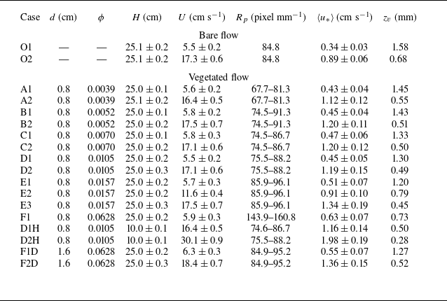
. The model vegetation characteristics are shown in table 1. Two water depths (
 $H$
= 10 and 25 cm) were considered. For each canopy configuration, one to three flow discharges were chosen, producing 18 cases (table 1). Additionally, two cases of bare flow were conducted for comparison. The channel-average velocity
 $U$
ranged from 5.5 to 30.1 cm s−1, which was consistent with field conditions (Leonard, Hine & Luther Reference Leonard, Hine and Luther1995; Naden et al. Reference Naden, Rameshwaran, Mountford and Robertson2006; Xu et al. Reference Xu, Esposito, Beltram-Burgos and Nepf2022).
(a) Photograph of both cylinder sizes. (b) Schematic top view of the canopy. Black dots indicate the position of individual cylinders. Grey triangles are Vectrino measurement locations. Green dashed lines represent laser planes. The red dashed box locates a unit cell that represents the repeated velocity pattern within the array. (c) Schematic of the weighting scheme in (3.2). If the weight of each black box is 2, the weighted contribution of Y1, Y2, Y3 and Y4 to the average over unit cell (red box) is 1, 2, 2 and 1, respectively. (d) A particle image in the Y4 lateral section captured by the high-speed camera. (e) The instantaneous flow field obtained from a pair of images in the Y4 section using the PIV-PTV method. Red and green dots denote the particle centroids identified in the first and second frames, respectively. Yellow arrows indicate the corresponding velocity vectors obtained through particle tracking.

Summary of experimental conditions and image resolution. The uncertainty in water depth
 $H$
arose from water surface fluctuations. Channel-average velocity
 $U$
was determined from the flow meter (i.e.discharge
 $Q$
) and the uncertainty reflects small fluctuations in flow meter readings. The friction velocity
 $\langle u_*\rangle$
uncertainty stemmed from repeated velocity measurements and fitting of velocity gradients within the viscous sublayer.

3.2. Measurements
A Nortek Vectrino measured the three-dimensional, instantaneous velocity
 $(u, v, w)$
. Vertical profiles started at
 $z=0.5$
cm and spanned the whole flow depth with a resolution of 1 cm. Four lateral positions (Y1–Y4, figure 2
b) between the stem rows (
 $x=4.0$
m, figure 1) were chosen to capture the lateral variation and to estimate the horizontal-average velocity within the canopy. Additional details for the Vectrino measurements can be found in Xu & Nepf (Reference Xu and Nepf2020, Reference Xu and Nepf2021).
To measure near-bed velocity at higher spatial resolution, we employed a method that combines PIV and PTV (i.e.hybrid PIV–PTV algorithm). The streamwise and vertical velocity
 $(u, w)$
was measured in the near-bed region in four planes, denoted by green dashed lines in figure 1. A 1.0-mm-thick continuous laser sheet with an energy of 20 w and a wavelength of 532 nm illuminated the near-bed region in the
 $x$
–
 $z$
plane. Hollow glass beads (Dantec Dynamics, HGS-10) with a mean diameter of 10
 $\unicode{x03BC}$
m and a density of
 $1.06\times 10^{3}$
kg m
 $^{-3}$
were used as tracer particles. The particle images were recorded by a high-speed CMOS camera (IDT OS II 3530,
 $2560 \times 1440$
pixels) through a macro lens (TAMRON SP AF 180 mm F/3.5 MACRO 1 : 1). The image resolution varied from 67.3 to 160.8 pixels mm−1 (table 1), corresponding to a field of view that ranged from 15.9 mm
 $\times$
9.0 mm (streamwise span
 $\times$
lateral span) to 38.0 mm
 $\times$
21.4 mm. Consistent with the Vectrino measurements, four lateral sections (
 $x$
–
 $z$
planes) within a unit cell (figure 2
b) were chosen to represent the velocity pattern within the array (Xu & Nepf Reference Xu and Nepf2020). The sampling frequency,
 $F_s$
, ranged from 400 to 1000 Hz, depending on the flow velocity. The frequency was high enough to resolve the small-scale turbulence. For each lateral section, a total of 12 000 images were recorded so that sufficient velocity vectors were available for statistical analysis. We repeated this one or two times for each case, producing 24 000–36 000 images for each section. The particle images (e.g. figure 2
d) were post-processed with the hybrid PIV–PTV algorithm. This algorithm first utilised a cross-correlation PIV algorithm developed by our group to compute a predictor displacement field for each image pair. The accuracy of the PIV algorithm has been validated in the fourth international PIV challenge (see results for case B from TsU in Kähler et al. Reference Kähler, Astarita, Vlachos, Sakakibara, Hain, Discetti, La Foy and Cierpka2016). Based on this field, the PTV algorithm was used to identify particle centroids via Gaussian-based particle masks and to track them using the relaxation algorithm (figure 2
e). The maximum displacement threshold, neighbourhood threshold, and quasi-rigidity threshold of the relaxation algorithm were determined automatically from the predicted displacement of each particle, as suggested by the predictor displacement field of PIV and previous studies (e.g. Kim & Lee Reference Kim and Lee2002; Chen et al. Reference Chen, Duan, Zhong, Wang and Huang2021). This hybrid PIV–PTV approach was well suited for the present experiment, given the high seeding concentration that ensured sufficient velocity vectors within the viscous sublayer (figure 2
a). This algorithm is presented in greater detail in the supplementary material is available at https://doi.org/10.1017/jfm.2025.11036. Based on the algorithm and high image magnification, the maximum vertical resolution of the near-bed flow field was
 $\Delta z \approx 0.02$
mm, which captured detailed velocity profiles very near to the bed. To the authors’ knowledge, the data acquired in this study has the highest vertical resolution of any vegetated flow experiments (see table S1 in the supplementary material, e.g. Liu et al. Reference Liu, Dumas, Fairbanks and Hodges2008; Yang et al. Reference Yang, Kerger and Nepf2015; Ricardo et al. Reference Ricardo, Franca and Ferreira2016; Conde-Frias et al. Reference Conde-Frias, Ghisalberti, Lowe, Abdolahpour and Etminan2023).
The time-averaged velocity was estimated as
 \begin{align} \overline {u} = \left ( \sum _{1}^{N} u \right ) / N, \qquad \overline {v} = \left ( \sum _{1}^{N} v \right ) / N, \qquad \overline {w} = \left ( \sum _{1}^{N} w \right ) / N, \end{align}
in which
 $N$
is the number of instantaneous velocity measurements. The horizontally averaged streamwise velocity
 $\langle \overline {u}\rangle$
was calculated as
 \begin{align} \langle \overline {u}\rangle =\left (\sum _{1}^{M}\omega _{i}\overline {u}\right )\Bigg/\left (\sum _{1}^{M}\omega _{i}\right )\!, \end{align}
in which
 $M$
is the number of time-averaged velocity data at height
 $z$
and
 $\omega _{i}$
is the weight of different lateral sections. As illustrated in figure 2(c), if the weight of each black box is 2, the weighted contribution of sections Y1, Y2, Y3 and Y4 to the average over unit cell (red box) is
 $\omega _{1} : \omega _{2} : \omega _{3} : \omega _{4} = 1 : 2 : 2 : 1$
.
The channel-average velocity
 $U$
was estimated by
 \begin{align} U=Q/\left [ \textit{WH}(1-\phi ) \right ] ,\end{align}
in which
 $Q$
is the channel discharge,
 $W$
is the channel width and
 $H$
is the water depth.
In the viscous sublayer the viscous stress
 $\tau _{v}$
was equal to the bed shear stress
 $\tau _{b}$
,
 \begin{align} \langle \tau _{b} \rangle = \langle \tau _{v} \rangle \big |_{z\lt z_{v}} = \rho \nu \frac {{\rm d}\langle \overline {u}\rangle }{{\rm d}z}\bigg |_{z\lt z_{v}}, \end{align}
from which the friction velocity
 $u_*=\sqrt {\tau _{b}/\rho }$
. The viscous sublayer thickness
 $z_{v}$
was determined before applying (3.4) using the following method. The five points closest to the bed, and including zero velocity at the bed, were linearly fit to obtain the velocity gradient,
 $k_v$
. The deviation of each measured velocity from the fitted line was calculated sequentially as
 \begin{align} E_{v} = \left | \frac {\langle \overline {u}\rangle _{n} - k_{v}z_{n}}{k_{v}z_{n}} \right | \times 100\,\% ,\end{align}
with
 $n=1, 2, 3, \ldots$
at increasing distance from the bed. When
 $E_{v}$
at point
 $n$
exceeded 3.5 % (Chen et al. Reference Chen, Duan, Zhong, Wang and Huang2021), the position
 $z_n$
was defined as the upper bound of the viscous sublayer.
The Reynolds stress
 $\langle \tau _R \rangle$
was calculated as
 \begin{align} \langle \tau _R \rangle =-\rho \langle \overline {u'w'} \rangle, \end{align}
in which the horizontal average (denoted by brackets) was similar to (3.2) and the overbar denoted a time average, defined in (2.1). The dimensionless Reynolds stress was defined as
 $-\langle \overline {u'w'} \rangle ^+ = -\langle \overline {u'w'} \rangle / \langle u_{*} \rangle ^2$
. The turbulent mixing length
 $l_r$
was estimated using (2.14):
 \begin{align} l_r = \frac {-\langle \overline {u'w'} \rangle ^{1/2}}{{\rm d}\langle \overline {u} \rangle /{\rm d}z} .\end{align}
The dimensionless mixing length was defined as
 $l_r^+ = l_r \langle u_* \rangle / \nu$
.
The dispersive stress
 $\langle \tau _d \rangle$
was calculated as
 \begin{align} \langle \tau _d \rangle = -\rho \langle \overline {u}'' \overline {w}'' \rangle, \end{align}
in which
 $\overline {u}''$
and
 $\overline {w}''$
were calculated using (2.2).
The vegetation drag coefficient
 $C_d$
was estimated using the Etminan, Lowe & Ghisalberti Reference Etminan, Lowe and Ghisalberti2017 model, i.e.
 \begin{align} C_d = \left ( \frac {1 - \phi }{1 - \sqrt {2\phi /\pi }} \right )^{2} \left [ 1 + 10\,\textit{Re}_d^{-2/3} \left ( \frac {1 - \phi }{1 - \sqrt {2\phi /\pi }} \right )^{-2/3} \right ]\!, \end{align}
in which
 $ \textit{Re}_d$
is the stem Reynolds number, defined as
 $ \textit{Re}_d = Ud / \nu$
.
3.3. Data verification
To validate the methods, measurements from the hybrid PIV-PTV method were compared with Vectrino measurements. In addition, the measurements made for bare flow conditions were compared with classic results from previous studies of bare flow. The velocity,
 $\overline {u}$
, at
 $z=0.5$
cm and four lateral positions (Y1–Y4) from Vectrino measurements were compared with those from PIV–PTV measurements (figure 3
a). The two methods show good agreement, with mean percent errors (MPEs) of only 3.7 %, indicating that the Vectrino and PIV-PTV measurements were both reliable and accurate.
(a) Comparisons of velocity,
 $\overline {u}$
, at
 $z=0.5$
cm for four lateral sections measured from Vectrino and the PIV-PTV method for both bare and vegetated cases. Panels (b), (c) and (d) show bare bed cases O1 and O2. (b) Dimensionless velocity profiles of bare cases (without vegetation) measured with the PIV-PTV method. The dashed and solid lines represent the linear velocity distribution (2.10) in the viscous sublayer and logarithmic law (2.15) in the turbulent layer, respectively. (c) Dimensionless Reynolds stress profiles. The grey dashed line represents the theoretical linear distribution. (d) Dimensionless turbulent mixing length profiles. The grey dashed line is the linear law (2.14).

Profiles of mean velocity,
 $\overline {u}$
, Reynolds stress,
 $\langle \tau _R \rangle$
, and mixing length,
 $l_r$
, from PIV-PTV measurements over a bare bed (O1 and O2) are shown in figure 3. The time-mean velocity profiles in the near-bed region follow the linear law (
 $z^+\lt 5$
, viscous sublayer) and classic logarithmic law (
 $z^+\gtrsim 30$
, turbulent layer, (2.15)), as illustrated in figure 3(b). The dimensionless Reynolds stress profiles were linear with
 $z$
in the outer layer (grey dashed line in figure 3
c). Moreover, the measured dimensionless mixing length
 $l_{r}^{+}$
(
 $l_{r}^{+}=l_{r}u_{*}/\nu$
) exhibited a linear relationship with
 $z^+$
(grey dashed line in figure 3
d), which was consistent with classic Prandtl mixing theory. The above comparisons further demonstrate the accuracy of the PIV-PTV method.
4. Results
4.1. Overview of the mean velocity profile
The vertical profile of temporally and horizontally averaged streamwise velocity,
 $\langle \overline {u}\rangle (z)$
, is shown in figure 4(a). The star and circle markers represent Vectrino and PIV–PTV measurements, respectively. Typically, the boundary layer thickness is defined as the height above the bed at which the velocity reaches 99 % of the free-stream velocity (Nowell & Jumars Reference Nowell and Jumars1984). However, this definition is inadequate for vegetated flows, because many profiles contain a velocity overshoot close to the bed, where the velocity exceeds the channel-average velocity
 $U$
(figures 4
a and 4
b). The velocity overshoot is connected to the secondary flow that develops near the cylinder base, consisting of a counter-rotating vortex pair that entrains high momentum fluid into the near-bed wake (also reported by Liu
 $et$
 $al.$
Reference Liu, Dumas, Fairbanks and Hodges2008 and Stoesser
 $et$
 $al$
. Reference Stoesser, Kim and Dumas2010). Thus, following Conde-Frias et al. (Reference Conde-Frias, Ghisalberti, Lowe, Abdolahpour and Etminan2023), for vegetated flow, we defined the boundary layer thickness,
 $z_\delta$
, as the height at which
 $\langle \overline {u}\rangle$
first reached the channel-averaged velocity
 $U$
(grey area of the inset graph in figure 4
b).
(a) Profiles of normalised velocity,
 $\langle \overline {u}\rangle /U$
, in vegetated cases A1, D1, F1, D1H and F1D. Star markers are Vectrino measurements. Small dots close to the bed are the PIV-PTV measurements. (b) An expanded view of the near-bed region for case D1H. The grey area denotes the boundary layer. The red dashed line indicates the top of the viscous sublayer (
 $z=z_v$
). (c) Profiles of stress gradients,
 $\partial \langle \tau _v \rangle /\partial z$
,
 $\partial \langle \tau _{R} \rangle /\partial z$
,
 $\partial \langle \tau _{d}\rangle /\partial z$
and vegetation drag,
 $F_{x}$
, as in (2.5) for case D1H.

Figure 4(c) shows the profiles of stress gradients
 $\partial \langle \tau _v \rangle /\partial z$
,
 $\partial \langle \tau _{R} \rangle /\partial z$
,
 $\partial \langle \tau _{d}\rangle /\partial z$
and the vegetation drag term
 $F_{x}$
in (2.5) for case D1H. Above the boundary layer (
 $z \gt z_\delta$
) the flow resistance was dominated by vegetation drag (figure 4
c), which balanced the net pressure force driving the flow. Approaching the bed, the flow resistance was dominated by the stress gradients (figure 4
c), which also balanced the pressure gradient. Because the pressure gradient is not a function of vertical position, we can approximate
 $F_x(z\gt z_\delta ) \approx \partial \langle \tau \rangle / \partial z$
(
 $z\lt z_\delta$
). By assuming that the stress gradient approaching the bed is dominated by viscous stress, i.e.
 \begin{align} \rho C_d a U^2 \approx \rho \nu \left . \frac {\partial ^2 \langle \overline {u} \rangle }{\partial z^2} \right |_{z\lt z_\delta } \sim \rho \nu \left . \frac {U}{z_\delta ^2},\right . \end{align}
we can predict the boundary layer thickness as
 \begin{align} \frac {z_\delta }{d} \sim \frac {1}{\sqrt {C_d a d}\sqrt {\textit{Re}_d} }, \end{align}
where
 $ \textit{Re}_d = Ud/\nu$
. The measured boundary thickness
 $z_\delta /d$
had a strong correlation with
 $1/\sqrt {\textit{Re}_d C_d a d}$
(
 $R^2 = 0.94$
, figure 5
a), indicating that (4.2), with scale constant
 $1.7 \pm 0.3$
(SD, standard deviation), provides a robust, new prediction of boundary layer thickness. Additionally, (4.2) also produced good agreement with measured boundary layer thickness from the previous study (Conde-Frias et al. Reference Conde-Frias, Ghisalberti, Lowe, Abdolahpour and Etminan2023), with a MPE of 17.8 % (figure 5
b).
Plots of
 $z_\delta /d$
versus
 $1/\sqrt {\textit{Re}_d C_d a d}$
from (a) the present study and (b) the previous study (Conde-Frias et al. Reference Conde-Frias, Ghisalberti, Lowe, Abdolahpour and Etminan2023). Best fit shown with the dashed grey line in (a).

Away from the bed,
 $z/H\gt 0.1$
, the velocity profiles,
 $\langle \overline {u} \rangle (z)$
, with and without vegetation were markedly different. Without vegetation, the velocity profile followed the classic logarithmic law (figure 3
b). However, within the model canopy, the velocity profiles was vertically uniform (figure 4
a), consistent with the uniform morphology of the model vegetation (rigid cylinders). In canopies with vertical variation in the plant frontal area and thus drag, the velocity varies inversely with the plant frontal area (Lightbody & Nepf Reference Lightbody and Nepf2006). In the outer region (i.e. above the boundary layer) of vegetated cases, the contribution of vegetation drag to the momentum balance (2.5) was significantly larger than the other terms (figure 4
c), which was also observed in Tinoco (Reference Tinoco2011) and Xu & Nepf (Reference Xu and Nepf2020). Therefore, this outer region was defined as the vegetation drag layer. In this region, (2.5) can be simplified to a balance between vegetation drag and pressure forcing, from which an inverse relationship between velocity distribution,
 $\langle \overline {u} \rangle$
, and frontal area,
 $a(z)$
, can be established (see Equation 21 in Xu & Nepf Reference Xu and Nepf2020), i.e.
 \begin{align} \frac {\langle \overline {u} \rangle }{U} = \sqrt {\frac {\langle a \rangle _z}{a(z)}}, \end{align}
in which
 $\langle a \rangle _z$
is the depth-averaged frontal area.
4.2. Mean velocity profile in the viscous sublayer
Mean velocity profiles within 2.5 mm of the bed are shown in figure 6 for different vegetation densities (
 $\phi = 0$
, 0.0039, 0.0105, 0.0628) and diameters (
 $d = 0.8$
, 1.6 cm). Notably, for vegetated conditions,
 $\langle \overline {u} \rangle$
exhibited a linear distribution near the bed (i.e.
 $z\ \lesssim \ 0.3$
–
 $1.5 \text{ mm}$
), similar to bare flow conditions (solid star in figure 6). The presence of a linear velocity distribution confirmed that viscous stress dominated the momentum balance at the bed, even when vegetation-generated turbulence was present, and a classic viscous sublayer (
 $u^+=z^+$
, in which
 $u^+ = \langle \overline {u} \rangle / \langle u_*\rangle$
and
 $ z^+ = z \langle u_*\rangle / \nu$
for vegetated cases) applies in vegetated flows. Individual time-mean profiles,
 $\overline {u}(z)$
, also exhibited a linear near-bed structure (data not shown).
Vertical profiles of time- and horizontal-mean velocity (
 $\langle \overline {u} \rangle$
) near the bed (
 $z \lt 2.5$
mm) measured from the PIV–PTV method. The blue and red markers indicate velocity ranges 5.5–6.3 cm s−1 and 16.4–18.4 cm s−1, respectively. Increasing SVF noted with a dashed arrow. The blue and red dashed lines indicate the velocity gradients in the viscous sublayer. The grey dashed line indicates the top of the viscous sublayer for case O1.

The thickness of the viscous sublayer,
 $z_v$
, was defined by the extent of the linear region of the near-bed velocity profiles (see figure 6 and § 3.2). Consistent with bare bed conditions (e.g. Nezu & Nakagawa Reference Nezu and Nakagawa1993; Dey Reference Dey2014),
 $z_{v}$
decreased with increasing channel-average velocity (figure 7
a). Importantly, the viscous sublayer thickness was also influenced by stem density, measured by the SVF,
 $\phi$
(figure 7
a). Specifically, for similar channel-average velocity and the same stem diameter, the sublayer thickness decreased with increasing SVF (dashed lines in figure 7
a). For example, for the bare bed (O1,
 $\phi =0$
in figure 7
a),
 $z_v = 1.71$
mm, which was 2.4 times the value for the most dense vegetated case (F1), for which
 $z_v = 0.70$
mm. The wake-generated turbulence mixed high momentum fluid downward toward the boundary, which depressed the viscous sublayer and elevated the near-bed velocity, compared with bare conditions. Specifically, the normalised velocity
 $\langle \overline {u} \rangle /U$
in the region
 $z^{+} \lt 60$
was higher for vegetated conditions, compared with the bare bed (see figure S2 in the supplementary material). The role of vegetation-generated turbulence in transporting higher momentum fluid toward the bed was also used to explain the thinning of the viscous layer (
 $H_v$
) discussed in Yang et al. (Reference Yang, Kerger and Nepf2015), Etminan et al. (Reference Etminan, Ghisalberti and Lowe2018) and Conde-Frias et al. (Reference Conde-Frias, Ghisalberti, Lowe, Abdolahpour and Etminan2023).
(a) The variation in the sublayer thickness,
 $z_v$
, with SVF,
 $\phi$
. Bare bed conditions correspond to
 $\phi = 0$
(star symbol). Blue and red markers indicate velocity ranges from 5.5 to 6.3 cm s−1 and from 16.4 to 18.4 cm s−1, respectively. The dashed lines are fitted curves between sublayer thickness and
 $\phi$
at similar velocity. (b) The variation of the normalised friction velocity,
 $\langle u_* \rangle /U$
, with SVF,
 $\phi$
. The legend is the same as figure 6.

Notably, the stem diameter also influenced
 $z_v$
. Specifically, for
 $\phi = 0.0628$
and a similar velocity (6 cm s−1), a larger
 $z_v$
was measured with the larger diameter (
 $d = 1.6$
cm, case F1D), compared with the smaller diameter (
 $d = 0.8$
cm, case F1, figure 7
a). This may be due to the fact that, for the same SVF, a larger diameter generated larger coherent structures, whose associated peak in turbulence was located farther from the bed, allowing a larger viscous sublayer to develop. Finally, the water depth had little effect on sublayer thickness in vegetated cases. Specifically, compare cases D1H (
 $H=10$
cm) and D2 (
 $H=25$
cm), which had the same velocity and SVF, but different depths (table 1). The sublayer thickness was the same within uncertainty,
 $z_v = 0.50 \pm 0.04$
and
 $0.49 \pm 0.03$
(SD), respectively.
Consistent with the decreasing thickness of the viscous sublayer, the friction velocity,
 $u_*$
, increased as vegetation density increased (figure 7
b). Specifically, for the most dense vegetated case (F1,
 $\phi =0.0628$
in figure 7
b),
 $\langle u_* \rangle /U$
was nearly twice the value for the bare bed (O1, blue star in figure 7
b), which resulted in a nearly four-fold increase in bed stress. It is worth noting that this is the first time that the viscous sublayer of vegetated flows has been directly measured in laboratory experiments. This is because previous experiments lacked sufficient vertical resolution, which prevented the acquisition of detailed measurements in the very near-bed region of vegetated flows (e.g.
 $z\lt 0.5$
mm).
When
 $\langle \overline {u} \rangle$
and
 $z$
were normalised using the inner variables
 $u_*$
and
 $\nu$
, all velocity profiles (bare and vegetated) collapsed onto a single line approaching the bed (figure 8
a). This makes sense, because, by definition, within the viscous sublayer the velocity profile is only dependent on viscosity and bed stress, resulting in
 $u^+=z^+$
. Notably, for both bare and vegetated cases, the viscous sublayer extended over the same non-dimensional range from
 $z^+=0$
to
 $z^+\approx \ 6$
, which was consistent with previous bare bed studies (e.g.
 $z_v^+=5$
, Nezu & Nakagawa Reference Nezu and Nakagawa1993). This suggested that the damping of turbulence by viscous stress at the bed occurred over a similar length scale (
 $z^{+} = 6.1 \pm 0.7$
, SD), with no dependence on the length scale of the outer layer turbulence, which differed significantly between bare and vegetated conditions. Specifically, the integral length scale in the outer layer is of the order of 1/10th of the flow depth for bare beds (Nezu & Nakagawa Reference Nezu and Nakagawa1993) and of the order of the stem diameter for vegetated beds (Tanino & Nepf Reference Tanino and Nepf2008).
(a) Dimensionless velocity profiles in the very near-bed region (
 $z^+\lt 30$
) for all cases. Grey symbols correspond to bare bed conditions and coloured symbols correspond to vegetated conditions. The grey shaded area indicates the viscous sublayer, where the mean velocity distribution is linear. The black dashed line represents the linear velocity law,
 $u^+=z^+$
. (b) Dimensionless velocity profiles over
 $z^+\lt 300$
. The data are presented on a log-linear scale. For vegetated cases, only measured data in the boundary layer (
 $z \lt z_\delta$
) are shown. The black dashed-dotted line indicates the classic logarithmic law.

4.3. Stress distributions define velocity layers
Above the viscous sublayer, the measured velocity profile becomes more complicated. In the bare flow conditions (O1 and O2), the buffer layer and turbulent log layer are both present, with a transition at
 $z^+= 30$
(figure 3
b), which was consistent with theory and previous studies (e.g. Nezu & Nakagawa Reference Nezu and Nakagawa1993; Dey Reference Dey2014). In vegetated conditions the dimensionless velocity deviated from the bare flow at
 $z^+= 13$
, within the traditional buffer layer (figure 8
b). Based on this, for vegetated flow, we divided the buffer layer into two parts, i.e.
 $6\lt z^+\le 13$
and
 $z^+\gt 13$
, which we named multi-stress layer I and multi-stress layer II, respectively (figure 10). The velocity distribution in each of these two layers is analysed below.
The velocity distribution is influenced by three stresses (2.5). Figure 9 compares the vertical profiles of viscous stress, Reynolds stress and dispersive stress over the region
 $z^+ \lt 60$
. In bare bed conditions, the dispersive stress
 $\tau _d$
(grey markers in figure 9
a) was negligible. The viscous stress (blue in figure 9
a) was constant in the viscous sublayer,
 $z^+\lt 6$
, and decreased rapidly with increasing distance from the bed above this point. For
 $z^+\gt 30$
, the contribution of viscous stress was less than 10 % of the total stress, and was considered negligible compared with the Reynolds stress. The Reynolds stress (red in figure 9
a) was negligible in the viscous sublayer, but increased sharply at
 $z^+\approx 6$
, reaching a maximum around
 $z^+\approx 25$
(as shown in figure 3
c).
Vertical profiles of the three stress components (
 $\langle \tau _v \rangle = \rho \nu \partial \langle \overline {u} \rangle / \partial z$
,
 $\langle \tau _R \rangle = -\rho \langle \overline {u' w'} \rangle$
,
 $\langle \tau _d \rangle = -\rho \langle \overline {u}'' \overline {w}'' \rangle$
) normalised by bed stress
 $\langle \tau _b \rangle$
within the near-bed region of (a) bare bed (cases O1 and O2), and (b) vegetated bed with all densities (cases A1–F1). The blue, red and grey markers represent viscous, Reynolds and dispersive stresses, respectively. The thick dashed line in (b) indicates the top of the boundary layer (
 $z^+ =z_\delta ^+=38$
) for case A1; and
 $z_\delta ^+ = 18$
for case F1. Note that, since the friction velocity was lower for bare cases, for the same physical distance from the bed (
 $z$
), the values of
 $z^+$
attain larger values, as reflected in the vertical axis range.

In vegetated flow the distribution of viscous stress
 $\langle \tau _v \rangle$
was similar to that in bare flow, with a maximum within the viscous sublayer and decreased rapidly with distance from the bed above the viscous sublayer (blue symbols, figure 9
b). However, in contrast to bare flow, for which dispersive stress
 $\langle \tau _d \rangle$
was negligible, in vegetated flow, dispersive stress (grey symbols) was comparable to Reynolds stress. For vegetated cases, both
 $\langle \tau _d \rangle$
and
 $\langle \tau _R \rangle$
were negligible in the viscous sublayer (
 $z^+\lt 6$
), then increased sharply above the viscous sublayer.
Schematic classification of the velocity layers for (a) emergent vegetated flows (layer thickness not shown to scale), and (b) bare flows. Here
 $z_\delta$
is the height of the boundary layer. In fully developed bare flows the boundary layer extends up to the water surface.

In multi-stress layer I (
 $6\lt z^+\le 13$
), both bare and vegetated conditions were dominated by viscous stress and Reynolds stress (figures 9
a and 9
b), which explains why the velocity within this layer of vegetated flow followed the same law as that in bare flow (figure 8
b). This corresponded to the buffer layer in bare conditions, which has been extensively investigated in previous studies (Dey Reference Dey2014). The buffer layer was thinner in the vegetated cases, extending to
 $z^+= 13$
, compared with bare flows, where it extended to
 $z^+=30$
(figure 10). The dimensionless velocity profiles in vegetated flow began to deviate from bare flows above
 $z^{+} = 13$
(figure 8
b), which was associated with a rapid increase in dispersive stress for
 $z^{+} \gt 13$
(figure 9
b). In this region, both Reynolds stress and dispersive stress were significant, defining multi-stress layer II (
 $13 \lt z^{+} \lt z_\delta ^{+}$
). Within this region the dimensionless velocity in vegetated flow was lower than that of bare flows (figure 8
b). Section 4.4.1 provides a detailed analysis of dispersive stress, confirming that
 $z^{+} = 13$
serves as the boundary between multi-stress layer I and II (see figure 13
b).
In summary, the velocity profile within an emergent canopy can be divided into four layers: the viscous sublayer, multi-stress layer I, multi-stress layer II and the vegetation drag layer (figure 10). Within the viscous sublayer (
 $z^+\le 6$
), only viscous stress is important, and the velocity distribution is linear. Within multi-stress layer I (
 $6 \lt z^+\le 13$
), both viscous stress and Reynolds stress are important, similar to the buffer layer of bare flows, resulting in the same velocity distribution in bare and vegetated conditions (figure 8). Within multi-stress layer II (
 $13\lt z^+\lt z_\delta ^+$
), Reynolds stress and dispersive stress are significant. The region above the boundary layer,
 $z^+\gt z_\delta ^+$
, is the vegetation drag layer (see § 4.1) within which the velocity varies inversely with the plant frontal area, as has been described in previous studies (e.g. Tinoco Reference Tinoco2011; Xu & Nepf Reference Xu and Nepf2020). For comparison, the canonical velocity structure in bare flow is presented in figure 10(b).
Although the main objective of this study was the near-bed region, the shear stress (
 $\langle \tau _R \rangle$
and
 $\langle \tau _d \rangle$
) distributions above this region are also of considerable interest. Within the boundary layer, the Reynolds stress
 $\langle \tau _R \rangle$
initially increased with distance from the bed and then decreased (figures 9
b and 10), which was consistent with the reduction in velocity shear near the top of the boundary layer (figure 9
b). Within an emergent canopy, the Reynolds stress is negligible over most of the flow depth (e.g. Nepf & Vivoni Reference Nepf and Vivoni2000), so that the Reynolds stress profile is expected to decrease toward zero above the measured region (i.e. in the vegetation drag layer) presented in figure 10 (see also figure 4c in Ricardo et al. Reference Ricardo, Franca and Ferreira2016). The dispersive stress
 $\langle \tau _d \rangle$
increased with distance from the bed throughout the boundary layer and continued to increase for some distance above the boundary layer (figure S5 in the supplementary material). The dispersive stress originates primarily from the secondary flow and wake structures at the intersection of an individual stem and the bed, i.e. the horseshoe system and wake region (figure S3c). The dynamic pressure gradient on the up- and downstream face of each stem, associated with the near-bed shear, generates persistent vertical velocity (Nepf & Koch Reference Nepf and Koch1999) from which much of the dispersive stress is derived. Specifically, the positive vertical velocity downstream of a stem (figure S3a) carries the low velocity fluid within the wake upward, producing a negative dispersive momentum flux (
 $ \overline {u}'' \overline {w}'' \lt 0$
). Because these regions of vertical velocity, and thus, the dispersive stress, are linked to the mean vertical shear, they are diminished with increasing distance from the bed, as the vertical shear weakens. Consequently, the dispersive stress within the vegetation drag layer is expected to decrease and approach zero at some height above the bed (figure 10, see also figure 5c in Ricardo et al. Reference Ricardo, Franca and Ferreira2016).
4.4. New velocity law in near-bed region of vegetated flow
For
 $z^+\gt 13$
, the velocity distribution in vegetated flows deviated from the classic logarithmic law. In this section a new velocity law for this region of vegetated flow is developed, starting with a modification of the Prandtl mixing theory to account for dispersive stress.
4.4.1. Modification of the Prandtl mixing theory for dispersive stress
Two key assumptions are made in the derivation of the classic logarithmic velocity law for bare beds. First, the turbulent mixing length
 $l_r$
is assumed to be proportional to the distance from the bed, i.e.
 $l_r=\kappa z$
. Second, the total shear stress is assumed to be equal to the bed shear stress. Since dispersive stress is negligible in bare conditions,
 $\langle \tau _{\textit{total}} \rangle = -\rho \langle \overline {u'w'}\rangle |_{z \to 0} = \langle \tau _b \rangle = \rho \langle u_*\rangle ^2$
. Both of these assumptions are modified in the presence of vegetation.
First, consider the mixing length. The mixing length measured for bare beds in this study (figure 11) followed a linear dependence
 $l_r^+=\kappa z^+$
above the buffer layer, i.e.
 $z^+\gt 30$
(grey dashed line), which was consistent with the measured logarithmic profile in this region (figure 3
b). Within the buffer layer,
 $z^+\lt 30$
, the mixing length followed a quadratic law (figure 11). This was consistent with the mixing length proposed by van Driest (Reference van Driest1956), which includes the buffer layer. Specifically, van Driest (Reference van Driest1956) described the additional damping of eddies by viscous stresses at the bed surface, arriving at the following mixing length profile for bare beds:
 \begin{align} l_r^+ = \kappa z^+\left [1 - \exp \left (-\frac {z^+}{B}\right )\right ]\!. \end{align}
Here
 $B$
is a constant with fitted value
 $B=26$
, which describes the dimensionless length scale (
 $z^+\lt B$
) over which eddies are further restricted by viscous effects approaching the boundary. Note that (4.4) reduces to
 $l_r^+=\kappa z^+$
at large
 $z^+$
. For bare conditions, the measured mixing length agreed with (4.4) both within the buffer layer (
 $z^+\lt 30$
, black dashed line in figure 11) and above it (
 $z^+\gt 30$
), where
 $l_r^+=\kappa z^+$
was observed (grey dashed line in figure 11).
Variation of dimensionless turbulent mixing length
 $l_r^+$
with
 $z^+$
in bare flow.

For vegetated conditions, the mixing length
 $l_r^+$
followed the van Driest (Reference van Driest1956) function, but with different values for
 $\kappa$
and
 $B$
. Specifically, considering all vegetated cases,
 $\kappa = 1.05$
and
 $B = 92$
(black dashed line in figure 12
a). Both values were larger than the corresponding bare bed values. The larger value of
 $\kappa$
could be attributed to vegetation stems contributing larger-scale turbulent eddies near the bed, especially within
 $z \lt d$
. The larger value of
 $B$
could reflect additional viscous damping on vegetation surfaces, which extends the region in which eddies are restricted by viscous effects approaching the boundary layer to a larger range of
 $z^+$
. Specifically, for
 $z_\delta ^+\lt B$
, (4.4) can be simplified using the Taylor series (green dashed line in figure 13
a):
 \begin{align} l_r^+ = \frac {\kappa }{B} z^{+2} = 0.011z^{+2}. \end{align}
Vegetated flow: dimensionless mixing length
 $l_r^+$
versus dimensionless distance from the bed
 $z^+$
. (a) All vegetated cases, with
 $z_\delta ^+$
ranged from 18 to 98. The grey and green dashed lines represent the linear and quadratic power law (4.5), respectively. The black dashed line represents the van Driest (Reference van Driest1956) function (4.4) with
 $\kappa =1.05$
and
 $B=92$
. (b) Lowest density case, case A. (c) Excluding case A. (d) Schematic of the mixing length variation with distance above the bed in bare (
 $\phi =0$
) and vegetated (
 $\phi \gt 0$
) flows.

(a) Dimensionless dispersive length
 $l_d^+$
in the boundary layer versus
 $z^+$
for vegetated cases. The black dashed line represents a quadratic relationship between
 $l_d^+$
and
 $z^+$
. (b) The relationship between
 $l_d^+/l_r^+$
and
 $z^+$
in the boundary layer. The horizontal line indicates the average value of
 $l_d^+/l_r^+$
for all vegetated cases.

The values of
 $\kappa$
and
 $B$
had some dependence on vegetation density. For the sparsest canopy (case A, SVF = 0.0039),
 $\kappa =0.51$
and
 $B=40$
(figure 12
b), close to the values observed in bare flows (
 $\kappa =0.41$
and
 $B=26$
). This makes sense, because we expect conditions to approach bare bed when the canopy is sufficiently sparse. For all other canopies (SVF
 $\geq 0.005$
),
 $\kappa =1.20$
and
 $B = 105$
(figure 12
c). The dependence on the SVF is summarised schematically in figure 12(d).
At sufficient distance from the bed, (4.4) reduces to the familiar linear dependence that leads to the logarithmic profile. For bare beds, a large fraction of the boundary layer exists within the limits of (4.4) that approximate the linear dependence. Specifically, under bare bed conditions (figure 11), the boundary layer contains mixing length scales that fit the van Driest full formulation close to the bed (
 $z^+ \lt 30$
) and also mixing length scales that reach the linear limit (
 $z^+ \gt 30$
), giving rise to the logarithmic profile.
The presence of vegetation influences the mixing length in two ways, reinforcing the quadratic scaling. First, turbulence produced in the vegetation wakes compresses the boundary layer thickness (i.e. figure 5), resulting in
 $z_\delta ^+\lt B$
, such that the entire boundary layer falls within the quadratic limit of (4.4), described by (4.5). In addition, since viscous damping occurs not only at the bed but also along the vegetation surfaces, the influence of viscous damping on mixing length size extends farther from the boundary. This is reflected in the increased value of
 $B$
in the van Driest function (see figure 12), relative to the bare bed value of
 $B$
. The larger value of
 $B$
allows the quadratic dependence for the mixing length to persist over the entire boundary layer,
 $z_\delta ^+\lt B$
, thereby reinforcing the quadratic scaling behaviour.
The second factor generating differences between bare and vegetated velocity profiles is the relative importance of different stresses. Specifically, in bare conditions only Reynolds stress is important above the viscous sublayer (figure 9 a), but for vegetated conditions, dispersive stresses are also significant (figure 9 b). Retaining the assumption that, close to the bed, the total shear stress can be approximated as a constant, for vegetated conditions,
 \begin{align} \langle \tau _{\textit{total}} \rangle = -\rho \langle \overline {u'w'} \rangle - \rho \langle \overline {u}''\overline {w}'' \rangle. \end{align}
In (4.6), Reynolds stress can be modelled using Prandtl’s mixing length (2.13). Although many studies have identified the importance of dispersive stress in gravel bed and vegetated flows (Dey & Das Reference Dey and Das2012; Fang et al. Reference Fang, Han, He and Dey2018; Kuwata & Kawaguchi Reference Kuwata and Kawaguchi2019; Rousseau & Angey Reference Rousseau and Angey2020), a closure model for dispersive stress has not been developed. Dispersive stress within a canopy primarily arises from the flow structures that form near the juncture of the bed and individual stems (Nepf & Koch Reference Nepf and Koch1999; Stoesser et al. Reference Stoesser, Kim and Dumas2010). Specifically, dispersive stresses are primarily associated with the region of upward vertical velocity (
 $\overline {w}'' \gt 0$
) present near the bed and directly behind each cylinder, where
 $\overline {u}'' \lt 0$
(Nepf & Koch Reference Nepf and Koch1999). This was confirmed by measurements made in the present study. Specifically, the terms
 $\overline {u}''$
,
 $\overline {w}''$
and
 $\overline {u}''\overline {w}''$
were primarily elevated in magnitude directly downstream of individual cylinders (see figure S3). Furthermore,
 $\overline {w}''$
was dominated by the upward velocity behind the cylinder (figure S3b), which we denote
 $w_{\textit{sf}}$
, for ‘secondary flow’. Nepf & Koch (Reference Nepf and Koch1999) show that
 $w_{\textit{sf}}$
is proportional to the gradient of the velocity squared
 $({\rm d} \langle \overline {u} \rangle ^2/{\rm d}z)$
, which for small gradients, can be approximated with
 $(d\langle \overline {u} \rangle /{\rm d}z)^2$
. Furthermore, because the streamwise velocity is close to zero in the cylinder wake, at this position
 $\overline {u}'' \sim \overline {u}$
; or, specifically,
 $\overline {u}'' \neq f({\rm d} \langle \overline {u} \rangle /{\rm d}z)$
. Given this, the dispersive stress is expected to scale as
 \begin{align} \langle \overline {u}'' \overline {w}'' \rangle \sim \left ( \frac {{\rm d} \langle \overline {u} \rangle }{{\rm d}z} \right )^2 \!. \end{align}
The similarity to the Reynolds stress closure (2.13), prompted us to consider
 \begin{align} -\langle \overline {u}'' \overline {w}'' \rangle \sim l_d^2 \left ( \frac {{\rm d} \langle \overline {u} \rangle }{{\rm d}z} \right )^2 \!, \end{align}
with a dispersive length,
 $l_d$
, defined in analogy to the turbulent mixing length. Velocity measurements were used to estimate the dispersive length based on (4.8). Specifically,
 \begin{align} l_d = \frac {-\langle \overline {u}''\overline {w}'' \rangle ^{1/2}}{{\rm d}\langle \overline {u} \rangle /{\rm d}z}. \end{align}
In the region
 $z^+\gtrsim 10$
, where dispersive stress was significant, the dispersive length varied quadratically with distance above the bed (
 $l_d^+ \sim z^{+2}$
), and this dependence extended up to the top of the boundary layer (figure 13
a). This was similar to the mixing length
 $l_r$
. In fact, the two mixing lengths were connected by a constant factor (figure 13
b),
 \begin{align} l_d^+ = k_d \, l_r^+, \end{align}
with
 $k_d = 1.35 \pm 0.32$
(SD).
4.4.2. New velocity law
The new closure for dispersive stress (4.8) was used to derive a velocity profile in multi-stress layer II (
 $13\lt z^+\le z_\delta ^+$
). Within this region, the total stress was assumed to equal the bed shear stress (see figure S6 and also figure 9 in Conde-Frias
 $et$
 $al$
. Reference Conde-Frias, Ghisalberti, Lowe, Abdolahpour and Etminan2023), and to be comprised of Reynolds and dispersive stresses, because viscous stress was negligible in this region (figure 9):
 \begin{align} \langle \tau _b \rangle = \rho \langle u_* \rangle ^2 = -\rho \langle \overline {u'w'} \rangle - \rho \langle \overline {u}''\overline {w}'' \rangle \sim \rho l_r^2 \left ( \frac {{\rm d} \langle \overline {u} \rangle }{{\rm d}z} \right )^2 + \rho l_d^2 \left ( \frac {{\rm d} \langle \overline {u} \rangle }{{\rm d}z} \right )^2 \!. \end{align}
Combining with (4.5) and (4.10), (4.11) can be simplified to
 \begin{align} \frac {{\rm d} \langle \overline {u} \rangle }{{\rm d}z} = \frac {\langle u_*\rangle }{\left ( \sqrt {1 + 1.35^2 }\times 0.011 \right ) z^2}. \end{align}
Integrating both sides and writing in terms of wall units,
 \begin{align} u^+ = -55.8/z^+ + C ,\end{align}
in which
 $C$
is an integration constant and
 $55.8 = 1/\sqrt {1 + 1.35^2 \times 0.011}$
. The integration constant
 $C=14.8$
was determined using a least squares of (4.13), which produced good agreement with measured data within multi-stress layer II
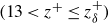 $(13\lt z^+\le z_\delta ^+)$
over all vegetated cases in the present study (figure 14
a). For individual cases, the MPE ranged from 0.7 to 5.3 %, with an average value of 2.4 %. The MPE was not corrected with the SVF or stem diameter. Figure 14(b) also includes near-bed velocity data provided in previous studies, which were obtained through experiment and LES simulation (grey markers, Etminan
 $et$
 $al$
. Reference Etminan, Ghisalberti and Lowe2018; Conde-Frias
 $et$
 $al$
. Reference Conde-Frias, Ghisalberti, Lowe, Abdolahpour and Etminan2023). Data from previous studies also agreed well with the new velocity law, with a MPE of 7.6 %. The new velocity law also performs well within multi-stress layer I (
 $6\lt z^+\lt 13$
, figure 15), where the velocity distribution was consistent with that in bare flow.
Comparison of measured velocity over the entire boundary layer (
 $z\le z_\delta$
) from (a) the present study and (b) previous studies with the new velocity law (4.13). The values of
 $z_\delta ^+$
in the present study ranges from 18 to 98. The black and grey dashed lines represent (4.13) and (2.10), respectively. The new power law (i.e. 4.13) applies to the region of
 $z^+\gt 13$
and
 $z\lt z_\delta$
.

The velocity profile should revert to a log layer for some low value of vegetation density. Based on the present study, the new power law velocity profile was a good description even at the lowest density,
 $\phi =0.0039$
, suggesting that the transition to a logarithmic profile occurs at a lower vegetation density. Given that the vegetation density in most natural environments exceeds this level (Gambi et al. Reference Gambi, Nowell and Jumars1990; Beltrán-Burgos et al. Reference Beltrán-Burgos, Esposito, Nepf, Baustian and Di Leonardo2023), the new power law can be widely applied in the field.
4.5. New methods to estimate bed shear stress in vegetated flow
In dimensional form, (4.13) is
 \begin{align} \langle \overline {u} \rangle = -\frac {55.8\nu }{z} + C\langle u_*\rangle .\end{align}
This velocity law extends to the top of the boundary layer in vegetated flows (figure 14), at which point
 $z= z_\delta$
and
 $\langle \overline {u} \rangle = U$
. Making these substitutions, the friction velocity can be estimated by
 \begin{align} \langle u_*\rangle = \frac {U}{C} + 3.8 \frac {\nu }{z_\delta }. \end{align}
The boundary layer thickness can be estimated from (4.2),
 $z_\delta = 1.7\sqrt {\nu /(C_d aU)}$
, allowing the friction velocity to be predicted from the channel velocity and canopy density:
 \begin{align} \langle u_*\rangle = \left ( C_v + 2.3 \sqrt {\frac {C_d a\nu }{U}} \right ) U, \\[-28pt] \nonumber \end{align}
 \begin{align} \langle \tau _b \rangle = \rho \langle u_*\rangle ^2 = \rho \left (C_v + 2.3 \sqrt {\frac {C_d a\nu }{U}} \right )^2 U^2 . \\[2pt] \nonumber \end{align}
Here
 $C_v=1/C$
and
 $C$
is a function of bed roughness. For the present study with a hydraulically smooth bed,
 $C_v=0.068$
. Equation (4.17) produced good agreement with vegetated cases in the present study (figure 15
a), with a MPE of 8.9 %, and from previous studies (Yang et al. Reference Yang, Kerger and Nepf2015; Etminan et al. Reference Etminan, Ghisalberti and Lowe2018; Conde-Frias et al. Reference Conde-Frias, Ghisalberti, Lowe, Abdolahpour and Etminan2023), with a MPE of 26.3 % (figure 15
b). As a reminder, the new model (4.17) estimates the spatially averaged bed shear stress. Due to the presence of vegetation, the bed shear stress has spatial variability (see figure S4) that is not captured by the present model.
(a) Measured (this study) and predicted bed shear stress. (c) Measured (previous studies) and predicted bed shear stress. Prediction from (4.17).

When
 $a=0$
(i.e.
 $\phi =0$
, bare flow), (4.15) reduces to
 $\langle u_*\rangle =C_v U$
, with
 $C_v=1/C =0.068$
in the present study. Here
 $C_v$
is not a universal constant and should reflect the bed roughness. For bare flows, previous studies describe a bed stress model for bare beds (e.g. Biron et al. Reference Biron, Robson, Lapointe and Gaskin2004), i.e.
 \begin{align} \langle u_* \rangle = \sqrt {C_{\kern-1.5pt f}} U ,\end{align}
where
 $C_{\kern-1.5pt f}$
is the bed drag coefficient, which is a function of bed roughness. It makes physical sense that
 $\sqrt {C_{\kern-1.5pt f}}$
and
 $C_v$
are related, as this results in a smooth transition from vegetated to bare conditions. We estimated the values of
 $\sqrt {C_{\kern-1.5pt f}}$
for cases O1 and O2 (bare cases) based on the measured
 $\langle \tau _b\rangle$
and
 $U$
, and found that
 $\sqrt {C_{\kern-1.5pt f}}=0.064$
and 0.059 for cases O1 and O2, respectively. These values are in close agreement with
 $C_v=0.068$
, confirming the physical connection between
 $C_v$
and
 $\sqrt {C_{\kern-1.5pt f}}$
.
The proposed bed shear stress model requires estimation of a vegetation drag coefficient
 $C_d$
, which is known through empirical relationships. Therefore, it is useful to understand the sensitivity of
 $\langle \tau _b\rangle$
to the choice of
 $C_d$
. From previous studies (Etminan et al. Reference Etminan, Lowe and Ghisalberti2017; Maza et al. Reference Maza, Adler, Ramos, Garcia and Nepf2017; Xu & Nepf Reference Xu and Nepf2020),
 $C_d$
is order one, so we considered the range 0.5–2.5. The deviation between measured
 $\langle \tau _{b,m}\rangle$
and predicted
 $\langle \tau _{b,p}\rangle$
with different
 $C_d$
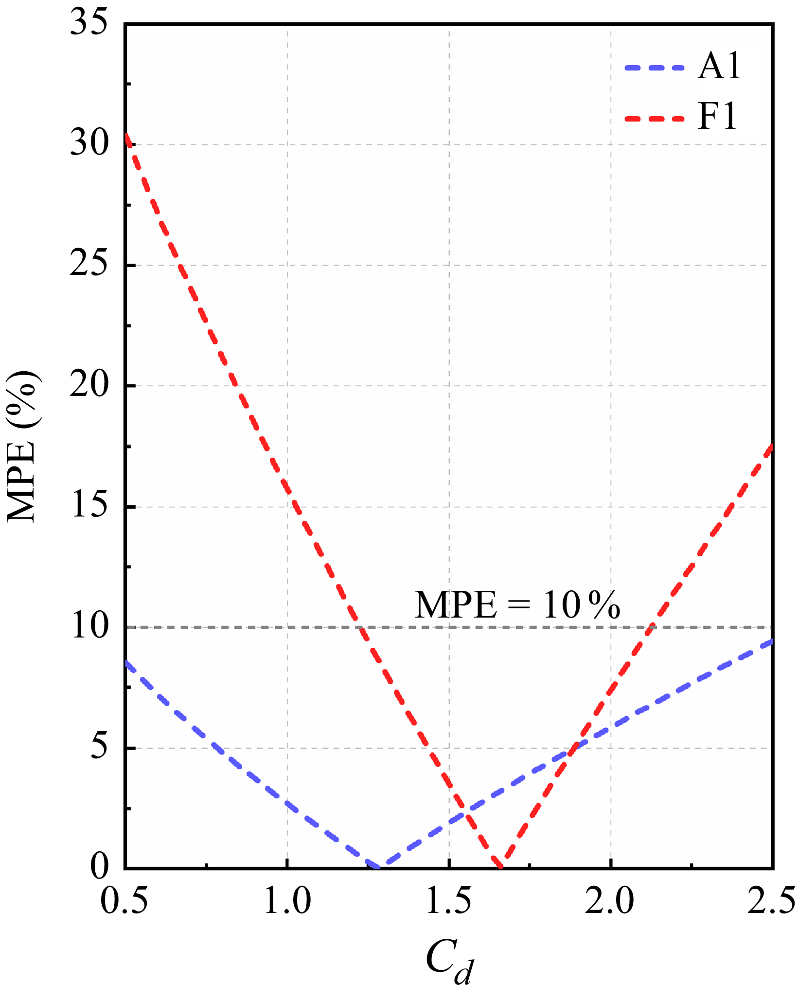
was evaluated using MPEs. For the sparsest canopy (A1), MPE
 $\lt$
10 % over the entire range of
 $C_d$
(figure 16). For the densest case (F1), the MPE reached 30 %, which suggests the low sensitivity of
 $C_d$
in a bed shear stress model. For field applications, this level of uncertainty would be comparable to the estimation of vegetation density.
Mean percentage error between predicted
 $\langle \tau _{b,p}\rangle$
and measured
 $\langle \tau _{b,m}\rangle$
with variation in parameter
 $C_d$
for the sparest (A1) and densest (F1) cases.

4.6. Limitation of new vegetated boundary layer model
Although this study was conducted using a regularly spaced array, the proposed model is expected to apply in irregularly spaced arrays. This expectation is based on the fact that the suppression of the boundary layer in vegetated flows is driven by vegetation-generated turbulence (e.g. Yang et al. Reference Yang, Kerger and Nepf2015; Etminan et al. Reference Etminan, Ghisalberti and Lowe2018; Conde-Frias et al. Reference Conde-Frias, Ghisalberti, Lowe, Abdolahpour and Etminan2023), and the spatially averaged, vegetation-generated TKE is similar for random arrays and regular arrays (Shan et al. Reference Shan, Zhao, Liu and Nepf2020). Furthermore, Ricardo et al. (Reference Ricardo, Franca and Ferreira2016) performed PIV measurements in two irregularly spaced canopy configurations. The vertical distributions of horizontally averaged velocity, Reynolds stress and dispersive stress in the near-bed region were consistent with those observed in the present study, indicating that similar patterns emerge in irregularly spaced arrays as in regular ones, once an appropriate horizontal averaging is applied. However, the extension of (4.16) and (4.17) to random or irregular stem arrays should be validated in future work.
The proposed model was shown to be valid within the vegetation density range
 $0.0039 \leqslant \phi \leqslant 0.25$
. This range encompasses typical vegetation densities observed in natural environments (e.g. Gambi et al. Reference Gambi, Nowell and Jumars1990; Manners et al. Reference Manners, Wilcox, Kui, Lightbody, Stella and Sklar2015; Beltrán-Burgos et al. Reference Beltrán-Burgos, Esposito, Nepf, Baustian and Di Leonardo2023; Li et al. Reference Li, Peng, Zhao, Fang, Chen, Xu and Wang2024), indicating that the new power law or bed shear stress model can be widely applied in the field. However, specific lower and upper critical density thresholds were not determined in this study and should be investigated in future work. Some simple analysis can provide criteria to define when the model may not be applicable. Let us first consider the lower bound of vegetation density (
 $\phi \lt 0.0039$
). When vegetation density becomes extremely sparse, the velocity profile should revert to a logarithmic distribution. Based on the present study, the new power law velocity profile was a good description even at the lowest density
 $\phi = 0.0039$
, corresponding to stem density
 $m$
= 78 stems m
 $^{-2}$
(with
 $d$
= 0.8 cm), suggesting that the transition to a logarithmic profile occurs at a lower vegetation density. The canopy density at which the transition to a logarithmic profile occurs can be inferred from the simplified momentum balance that led to (4.2). Specifically, the formulation of
 $z_\delta$
in (4.2) becomes invalid when the vegetation drag
 $F_v$
is comparable to or smaller than the bed shear stress
 $\langle \tau _b \rangle$
, i.e.
 $F_v = {\rho C_d \textit{aHU}^2}/{2(1 - \phi )} \leq \langle \tau _b \rangle$
. Using (4.17) to estimate
 $\langle \tau _b \rangle$
, a critical vegetation density
 $\phi _{c_1}$
can be identified. For example, consider a typical field condition with the water depth
 $H = 20$
cm, channel velocity
 $U$
= 0.1 m s−1 and stem diameter
 $d$
= 1.5 cm (e.g. reed or mangrove aerial roots). Because the canopy is sparse,
 $F_v \approx \rho C_d \textit{aHU}^2$
. Assuming that
 $C_d = 1$
(Nepf Reference Nepf2012),
 $F_v \leq \langle \tau _b\rangle$
corresponds to
 $a_{c_1}= 0.05$
m
 $^{-1}$
(
 $\phi _{c_1} = 0.0006$
), which is much lower than any case considered in this study. Alternatively, we can consider the transition in mixing length behaviour. Specifically, if the boundary layer is large compared with
 $B$
, i.e.
 $z_\delta ^+ \gg B$
, then within most of the boundary layer (4.4) is reduced to
 $l_r^+ \sim z^+$
, which will produce a logarithmic profile within the boundary layer, i.e. the flow will be similar to that of a bare bed. Accordingly, the critical vegetation density can be estimated by solving
 $z_\delta ^+ \gg B$
. Second, let us consider the upper range of density (
 $\phi \gt 0.25$
), the dominant turbulence length scale shifts from the stem diameter to the stem spacing (Tanino & Nepf Reference Tanino and Nepf2008). This transition may result in a different degree of turbulent mixing and spatial heterogeneity, potentially altering the magnitude of the Reynolds stress and dispersive stress.
Finally, the proposed model was developed with an emergent canopy and a hydraulically smooth bed. The extension to a submerged canopy or a rough sediment bed requires further validation. In submerged canopies, turbulence generated in the shear layer at the top of the canopy can be carried by turbulence transport toward the bed, which has been shown to enhance near-bed turbulence and bed load transport (King et al. Reference King, Tinoco and Cowen2012; Zhao & Nepf Reference Zhao and Nepf2024). If the additional turbulence alters the mixing length scale or further depresses the boundary layer, it could lead to deviations from the proposed velocity model. Similarly, bed roughness from grains or bedforms, both of which were excluded in the present study, can influence bed shear stress. We hypothesised that this effect would be captured by
 $C_v$
in (4.17), but this remains to be validated with experiments using rough beds.
5. Conclusions
A coupled PIV–PTV system was used to obtain high spatial resolution and high frequency velocity measurements in the near-bed region of emergent vegetated flows. Importantly, this was the first study of vegetated flows to measure the velocity profile within the viscous sublayer. The highly detailed profiles of velocity and stress produced several important findings. First, a viscous sublayer, with linear velocity profile, is present in vegetated flow and has the same non-dimensional thickness,
 $z^+=6$
, as bare flow. However, for the same channel velocity, the dimensional sublayer thickness in vegetated flow is significantly smaller than that in bare flow, producing higher bed shear stress. Second, unlike bare channels, the horizontally averaged velocity does not follow the classic logarithmic law in the boundary layer. Consistent with this, the turbulent mixing length,
 $l_r^+=\kappa z^+$
, does not hold within vegetated flow, because the thinning of the boundary layer precludes this scale of turbulence from emerging. Instead, the thickness of the vegetated boundary layer leads to a dominance of the very near-bed scaling defined by van Driest, i.e.
 $l_r^{+} \sim z^{+2}$
, with a constant scale coefficient of 0.011 across vegetation density
 $\phi = 0.0039$
–
 $0.0628$
. In addition, over the range of density considered, the dispersive stress was comparable to Reynolds stress and cannot be neglected. To account for this, a modified mixing length theory for vegetated flow was developed and used to derive a new near-bed velocity distribution. Based on the new velocity law and the definition of boundary layer thickness, the spatially averaged bed shear stress can be estimated from the channel-average velocity, vegetation parameters and vegetation drag coefficient
 $C_d$
, all of which, except
 $C_d$
, are easily measured in the field. Uncertainty analysis demonstrated that the uncertainties in
 $C_d$
are generally comparable to those in vegetation density under field conditions, which supports the robustness and practical applicability of the proposed model. Finally, the proposed model has been validated across a wide range of vegetation densities, with a SVF from 0.0039 to 0.25, corresponding to a stem density of
 $m$
= 78–4980 stems m
 $^{-2}$
for
 $d$
= 0.8 cm.
Supplementary material
Supplementary material is available at https://doi.org/10.1017/jfm.2025.11036.
Funding
This study was supported by the National Natural Science Foundation of China (grant no. 42576168, 52509095, U24A20181), Shanghai Sailing Program (23YF1410200), Natural Science Foundation of Shanghai Municipality (23ZR1420100), Open Research Fund Program of the State Key Laboratory of Hydroscience and Engineering (sklhse-KF-2025-E-03), Open Research Fund of Key Laboratory of Ocean Space Resource Management Technology, MNR (KF-2023-110).
Declaration of interests
The authors report no conflict of interest.