1 Introduction
A vortex ring is a torus shaped vortex in a fluid with a concentrated region of azimuthal vorticity in its core, surrounded by a region of irrotational flow. A circular vortex ring moves along its axis due to its self-induced velocity, a canonic property that has helped investigators to illustrate the formation, evolution and decay dynamics of axisymmetric vortex structures elegantly. Based on the ratio of core radius (
 $a$
) to vortex ring radius (
 $R$
), (
 $\unicode[STIX]{x1D700}=a/R$
) a vortex ring is termed as thin core (
 $\unicode[STIX]{x1D700}<0.1$
) or thick core (
 $\unicode[STIX]{x1D700}>0.1$
) (Fraenkel Reference Fraenkel1972).
The vortex ring is one of the most intensely investigated fluid dynamic structures as it can be generated easily and it helps in understanding the nature and dynamics of vortex structures in different physical environments. Its formation and propagation studies have provided much insight into the nature of vorticity containing fluid motion and subsequent instabilities. Yet the numerous ways in which vortex rings have been generated show differences in their evolution characteristics. Diversities in the observations of the nature of this interesting flow phenomenon have given rise to the development of much theoretical work aiming to predict their motion and to explain the discrepancies. The differences found in numerous experimental investigations, and also between these experiments and theoretical predictions, have been the subject of much research that has led to the enlisting of many explanatory models.
Vortex rings can be observed often in nature. Vortex rings form in the left ventricle of the human heart during cardiac relaxation, as a jet of blood enters through the bicuspid valve. Optimal vortex rings are used by aquatic creatures such as jellyfish to generate a propulsive force. Dolphins, beluga whales and humpback whales create air bubble rings for self-amusement. Vortex rings are also observed in volcanic eruptions. In engineering applications, vortex rings generate propulsive thrust in pulsed detonation engines, vortex guns use the property of self-induced velocity of the vortex ring to deliver fluid to large distances. The vortex ring is an integral part of a starting jet.
1.1 Methods of vortex ring generation and associated problems
In an experimental arrangement the first reported vortex ring formation was probably by Gengembre (Reference Gengembre1785). Subsequently, in the early nineteenth century, vortex rings were created experimentally by Faraday (Reference Faraday1847) and Babbage (Reference Babbage1864) (experiments were carried out in 1827 and 1828 respectively) and later on by Rogers (Reference Rogers1858). An account of the early observations and studies on vortex rings can be obtained from Fuentes (Reference Fuentes2014). In experiments, the most commonly adopted method of producing vortex rings is to eject a slug of fluid out of an orifice or nozzle with the help of an impulsively moving piston (Saffman Reference Saffman1970; Maxworthy Reference Maxworthy1977; Didden Reference Didden1979; Pullin Reference Pullin1979; Blondeaux & De Bernardinis Reference Blondeaux and De Bernardinis1983; Auerbach Reference Auerbach1987; Irdmusa & Garris Reference Irdmusa and Garris1987; Glezer Reference Glezer1988; Glezer & Coles Reference Glezer and Coles1990; Auerbach Reference Auerbach1991; Lim & Nickels Reference Lim and Nickels1995; Weigand & Gharib Reference Weigand and Gharib1997; Shusser & Gharib Reference Shusser and Gharib2000; Allen & Auvity Reference Allen and Auvity2002; Cater, Soria & Lim Reference Cater, Soria and Lim2004; Sullivan et al.
Reference Sullivan, Niemela, Hershberger, Bolster and Donnelly2008). The properties of such experimentally produced vortex rings are categorized on the basis of the features of generating apparatus. Thus, a thorough understanding of the underlying flow physics is required to interlink these results with the theoretical formulations that are based on mathematical concepts and physical quantities such as the core diameter, circulation, vortex ring diameter and self-induced translational velocity. The streamfunction and velocity potential of a vortex ring have been derived elegantly by Lamb (Reference Lamb1932). Tung & Ting (Reference Tung and Ting1967) considered the effects of viscosity in the inner core of the vortex ring; the inner viscous solution was matched with the classical inviscid solution of the outer region. An expression for the translational velocity of viscous vortex rings was derived by Saffman (Reference Saffman1970). He calculated the propagation velocity of a vortex ring with relatively small core size, constant diameter and a Gaussian distribution of vorticity inside the core. Later, Saffman (Reference Saffman1978), utilizing similarity theory (Kaden Reference Kaden1931) of the formation of a vortex at a two-dimensional sharp edge in an impulsively started flow, obtained the diameter and circulation of a fully formed vortex ring that was in good agreement with the experimental findings of Maxworthy (Reference Maxworthy1977). This was extended by Pullin (Reference Pullin1979) for an axisymmetric geometry. Fukumoto & Moffatt (Reference Fukumoto and Moffatt2000) obtained a large Reynolds number asymptotic solution of the Navier–Stokes equation for the motion of an axisymmetric vortex ring of small cross-section in a viscous incompressible fluid. They established a general formula for the translational speed of a vortex ring which is valid up to third order in
 $\unicode[STIX]{x1D700}$
.
Didden (Reference Didden1979) measured the vorticity flux during formation of vortex rings at the exit edge of a pipe and provided the explanation for the deviation from the prediction of vorticity flux by the slug flow model proposed by Maxworthy (Reference Maxworthy1977) based on the interaction of internal and external boundary layers. Maxworthy (Reference Maxworthy1977) and Didden (Reference Didden1979) observed that when the piston motion ceases, the primary vortex ring induces the formation of a secondary vortex ring of opposite circulation which is known as stopping vortex in today’s literature. Also, the measurements of vortex ring diameter obtained by Didden (Reference Didden1979) showed a decrease at the end of the piston stroke. The reasons attributed to this observation is the influence of the nozzle wall and the induced flow of the secondary vortex ring.
The role of the generating apparatus and the piston velocity history are very crucial in the evolution of vortex rings. Auerbach (Reference Auerbach1991) observed that for an abruptly stopped piston, a small ring of opposite vorticity to that of the primary ring is generated at the exit and moves upstream into the nozzle. The primary vortex ring reduces its diameter to its steady laminar size due to presence of the stopping vortex. Streamwise vortices are usually generated in the axisymmetric stagnation flow initiated on the translation axis outside the nozzle. Auerbach (Reference Auerbach1991) found that vortex rings contract to their final diameter by the time they move approximately
 $1.5L_{P}$
(stroke length) from the nozzle exit.
Experiments performed with the orifice geometry by Irdmusa & Garris (Reference Irdmusa and Garris1987) also indicate that vorticity of opposite sign to the primary vortex ring is generated on the wall of the orifice exit by the boundary layer formed due to the induced opposite directional flow over it during the stoppage of the driving piston. According to these authors, this causes a reduction in the net available vorticity forming the vortex ring. Development of a vortex ring due to rolling up of the boundary layers (Irdmusa & Garris Reference Irdmusa and Garris1987) is dependent on the generating apparatus and the initial behaviour of the vortex ring changes due to the same. An extensive work on the evolution characteristics of a vortex ring by Weigand & Gharib (Reference Weigand and Gharib1997) reveals that the contraction of the vortex ring to reach a stable diameter starts during the deceleration of the piston during which an opposite sign stopping vortex is seen to propagate into the tube. Didden (Reference Didden1979) states that the final non-dimensional diameter of the vortex ring is a function solely of
 $L_{P}$
(stroke length)
 $/D$
(vortex ring diameter) while Lim & Nickels (Reference Lim and Nickels1995) establishes its dependence on the geometry of the generator.
Production and generation of secondary vorticity has also been observed for rectilinear vortex pairs (Auerbach Reference Auerbach1987) that causes their motion to deviate from the similarity theory predictions (Pullin & Perry Reference Pullin and Perry1980). In this case also, if the flow is stopped abruptly, a second rectilinear vortex of opposite sign generates at the edge tends to contract the primary vortex pair (Blondeaux & De Bernardinis Reference Blondeaux and De Bernardinis1983).
In order to eliminate the production of secondary vorticity for the case of vortex rings, Glezer (Reference Glezer1988) as well as Glezer & Coles (Reference Glezer and Coles1990) used a vortex ring generating apparatus with the piston flushing with the wall upon completion of the stroke, forming a vortex ring near a plane wall and moving away from it. This method decreased the initial overshoot in the flux of vorticity into the vortex ring, and eliminated the effects of stopping vortex of opposite sign from the wall boundary layer. But, they also inadvertently introduced a piston vortex of same sign of circulation as of primary vortex ring into the flow (Cater et al. Reference Cater, Soria and Lim2004). This piston vortex is produced at the piston face as it scrapes the boundary layer from the inside of the cylinder.
Allen & Auvity (Reference Allen and Auvity2002) showed the contraction is almost identical for the case when the piston is stopped inside the tube, and hence a stopping vortex is formed, and the case when the piston finishes flush and the piston vortex is ingested. Thus they conclude that the vortex ring contraction is not a direct result of the system of images and stopping vortex but rather the vortex ring relaxing to its natural state, which is a function of its invariants. The generation geometry is important in terms of determining how these invariants are produced.
Cater et al. (Reference Cater, Soria and Lim2004) also showed that when the piston vortex is confined within the tube and far away from the exit, its influence on the primary vortex ring is small. However, if the piston vortex gets ejected into the flow, it changes the properties of the primary vortex ring by interacting with it. This interaction causes an increase in the circulation of the primary vortex ring and modifies the vorticity distribution and evolution of the vortex core.
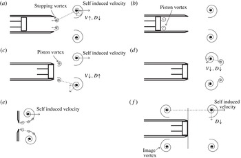
To summarize, the sketches of the general disturbances in nozzle and orifice configurations are shown in figure 1. These figures summarizing the findings of above investigations, certainly provide possible explanations to the observed behaviour of the evolution of vortex rings and the underlying physics. The present study is an effort to produce a ‘classical’ vortex ring free from all the above effects. This is achieved by minimizing the effects of the numerous factors influencing the predictions of evolution characteristics proposed by the vortex ring model by Tung & Ting (Reference Tung and Ting1967), Saffman (Reference Saffman1970) and Fraenkel (Reference Fraenkel1972). Thus, in this work an effort has been made to realize such a vortex ring practically through a novel generation mechanism and to bring out the significance of the observations made therein. Such classical vortex ring generated shows some interesting features of its propagation and dynamical characteristics. A well written document on the characteristics of vortex ring is by Sullivan et al. (Reference Sullivan, Niemela, Hershberger, Bolster and Donnelly2008) and the given properties are revisited with respect to the creation of the vortex ring free from all the above effects.
Sketches of (a) stopping vortex (Blondeaux & De Bernardinis Reference Blondeaux and De Bernardinis1983), (b) piston vortex during the formation phase (Allen & Auvity Reference Allen and Auvity2002), (c) piston vortex when the piston is full flushed (Allen & Auvity Reference Allen and Auvity2002), (d) piston vortex interacting with primary vortex (Allen & Auvity Reference Allen and Auvity2002), (e) disturbances in orifice generated vortex ring during the formation phase (Pedrizzetti Reference Pedrizzetti2010), and (f) image vortex (Allen & Auvity Reference Allen and Auvity2002).
 $D$
is the diameter and
 $V$
is the translational velocity of the vortex ring (solid arrow line represents self-induced velocity and dashed arrow line represents the induced velocity by another vortex or vortices).

1.2 Characteristics of incompressible vortex ring
A vortex ring is characterized by its diameter (
 $D$
), circulation (
 $\unicode[STIX]{x1D6E4}$
) and core radius (
 $a$
). The translational velocity (
 $V$
) can be written in terms of these parameters or alternatively by its impulse (
 $P$
) and energy (
 $E$
). The basic characteristics are largely available with some well-known models. The validity of these models and some other models as well as empirical relations available in literature will be discussed in detail in the context of the present study in § 4.
It can be easily shown that, for a vortex ring with constant circulation, the translational velocity and the impulse can be related by the Hamilton’s equation
 $$\begin{eqnarray}V=\frac{\unicode[STIX]{x2202}E}{\unicode[STIX]{x2202}P}.\end{eqnarray}$$
Considering the simplest situation, i.e. when the core radius is very small as compared to the vortex ring radius (
 $R$
) (
 $a\ll R$
), one can write (Sullivan et al.
Reference Sullivan, Niemela, Hershberger, Bolster and Donnelly2008)
 $$\begin{eqnarray}E=\frac{1}{2}\unicode[STIX]{x1D70C}\unicode[STIX]{x1D6E4}^{2}R\left(\ln \frac{8R}{a}-\unicode[STIX]{x1D6FC}\right)\end{eqnarray}$$
and
 $$\begin{eqnarray}V=\frac{\unicode[STIX]{x1D6E4}}{4\unicode[STIX]{x03C0}R}\left(\ln \frac{8R}{a}-\unicode[STIX]{x1D6FD}\right).\end{eqnarray}$$
Here,
 $\unicode[STIX]{x1D6FC}=2.04$
and
 $\unicode[STIX]{x1D6FD}=0.558$
(Donnelly Reference Donnelly1991) and
 $\unicode[STIX]{x1D70C}$
is the density of the fluid. For such a vortex ring, the impulse is also given as,
 $$\begin{eqnarray}P=\unicode[STIX]{x1D70C}\unicode[STIX]{x1D6E4}\unicode[STIX]{x03C0}R^{2}.\end{eqnarray}$$
If the core is assumed to be finite but small (finite but small values of the dimensionless core radius
 $\unicode[STIX]{x1D700}=a/R$
), the second-order formulas for impulse and energy are given by Fraenkel (Reference Fraenkel1972). For a Gaussian vorticity distribution in the core, an expression for the core radius is given by Saffman (Reference Saffman1970) as,
 $$\begin{eqnarray}a_{T}=\sqrt{4\unicode[STIX]{x1D708}T},\end{eqnarray}$$
where
 $\unicode[STIX]{x1D708}$
is the kinematic viscosity and
 $T$
is the stroke time of the piston. Fukumoto & Moffatt (Reference Fukumoto and Moffatt2000) considered the motion of a vortex ring in a viscous fluid starting from an infinitely thin circular loop of radius
 $R$
at
 $t=0$
and carried the formula given by Saffman (Reference Saffman1970) a step further. Weigand & Gharib (Reference Weigand and Gharib1997) studied the evolution of laminar vortex rings using laser Doppler anemometry (LDA) and digital particle image velocimetry measurements. The analysis of Saffman (Reference Saffman1970) for a viscous vortex ring is considered and it is shown that the velocity decays as,
 $$\begin{eqnarray}V\approx \frac{1}{k}(R^{2}+k^{\prime }\unicode[STIX]{x1D708}t)^{-2/3},\end{eqnarray}$$
where
 $k$
and
 $k^{\prime }$
are constants.
The basic assumption of the slug model (Maxworthy Reference Maxworthy1977; Didden Reference Didden1979) is that the vortex ring is formed from a cylindrical slug of fluid ejected from a nozzle with velocity
 $U_{0}$
. The expression for the slug model circulation is,
 $$\begin{eqnarray}\unicode[STIX]{x1D6E4}_{s}=\frac{L^{2}}{2T},\end{eqnarray}$$
where
 $L$
is the stroke length of the piston. Here, the stroke length used is an equivalent stroke length; as the dimensions of the piston used in the experiments are not the same as that of the nozzle exit, an equivalent stroke length is defined assuming the volume flow rate through the driving section and the nozzle exit to be same. Hence,
 $$\begin{eqnarray}L_{eq}=L_{P}\frac{A_{P}}{A_{0}},\end{eqnarray}$$
where
 $L_{P}$
is stroke length of piston,
 $A_{P}$
is the cross-sectional area of the piston and
 $A_{0}$
is the nozzle exit area.
 $A_{0}=\unicode[STIX]{x03C0}D_{0}^{2}/4$
, where
 $D_{0}$
is the nozzle exit diameter.
The validity of these models and other existing models are readdressed in § 4 as each model is different and the characteristic values obtained from them are different. The validity has been established with reference to the clean vortex ring data obtained in this study. The drawbacks and strengths of these models are discussed.
2 Experimental set-up
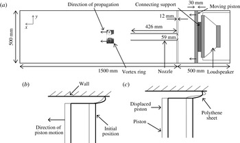
The experimental set-up used for generating a vortex ring is shown in figure 2. A large tank of a square cross-section of
 $0.5~\text{m}\times 0.5~\text{m}$
and length 2 m is divided into two parts (by a square plate 12 mm thick); the driver part of length 0.5 m contains the piston (made of thick light polystyrene foam sheet) that drives the flow and the other longer part of length 1.5 m consists of the nozzle (of inner diameter
 $D_{0}=59~\text{mm}$
), and the test section, where the vortex ring forms and propagates. A flat square shaped piston of cross-section
 $0.49~\text{m}\times 0.49~\text{m}$
is driven by a
 $100~\text{W}$
loudspeaker. The tank of large cross-sectional area compared to the vortex ring diameter provides a quiescent ambient fluid and also eliminates any effects of external air current on the experimental observations.
The piston dimensions are such that it closely fits the walls of the chamber. The small gap is sealed with the help of strips of polythene sheet in such a way that it allows the piston to move smoothly without rubbing against the surface of the wall and it also ensures a leak-proof arrangement. The gap between the piston and wall is approximately 5 mm and the maximum amount of fluid which can possibly be pushed by polythene sheet (assuming no deformation of the sheet due to back pressure, see figure 2 b) in this gap, as the piston moves forward, is approximately 0.4 % of the total volume of the fluid coming out of the nozzle. In reality, due to back pressure, the sheet deforms as shown in figure 2(c), which reduces the uncertainty in volume flow rate significantly lower than the above value.
(a) Schematic of the experimental set-up, (b) sheet deformation if no bulging is present due to back pressure, (c) expected sheet deformation due to back pressure.

The loudspeaker is driven by a signal that is initially synthesized and stored in the non-volatile memory of a function generator. The signal generation is triggered by a transistor–transistor logic (TTL) trigger signal from the NI-DAQ (NI USB 6210) card. This signal is amplified by a power amplifier and fed to the loudspeaker that drives the piston. The signal, used to drive the loudspeaker, is trapezoidal with smooth corners. The distance by which the piston moves is the stroke length (
 $L_{P}$
) and the time taken for the piston to move this distance is the stroke time (
 $T_{P}$
). Unlike commonly used piston–cylinder configurations for producing vortex rings, the present nozzle configuration does not have the piston inside the tube itself. Instead, the piston is in the driving section outside it. This eliminates the possibility of any piston vortex in the vicinity of the primary vortex ring. The nozzle (of 2 mm wall thickness) is mounted on the dividing plate centre as shown in the figure 2, is having a smooth chamfered entry and sharp exit. The length of the nozzle (426 mm) is chosen sufficiently large (also eliminates the possibility of image vortex effects as shown in figure 1
f) so that the slug of fluid that emerges from the nozzle exit is only from the front portion of it. Thus the slug of fluid does not contain any fluid from the entry region of the nozzle and eliminates the possibility of having disturbances similar to that of orifice generated vortex ring (see figure 1
e). The smooth entry also ensures minimization of disturbance pressure fluctuations at the entry. During the short period of unsteady flow (
 $T_{p}\approx 200~\text{ms}$
) inside the nozzle pipe boundary layer thickness (boundary layer thickness,
 $\unicode[STIX]{x1D6FF}_{bl}\approx 3.14\sqrt{\unicode[STIX]{x1D708}t}$
, see Das Reference Das1998) is approximately 5 mm. After piston stops, a reverse flow inside the nozzle pipe (Das & Arakeri Reference Das and Arakeri1998) is evident to satisfy zero mass flow condition at any cross-section inside the pipe. The reverse flow causes flow over the outer part of the sharp exit that generates a stopping vortex ring. To minimize the stopping vortex effect in the present study the piston is stopped gradually and slowly such that the reverse flow does not form a stopping vortex of large strength. An impulsive or rapid stop will always form the stopping vortex. These points are discussed in § 3 with quantitative data. These measures in designing the experimental set-up are important for generating a clean vortex ring.
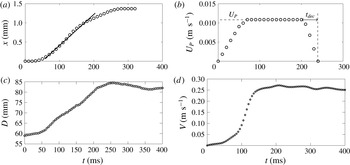
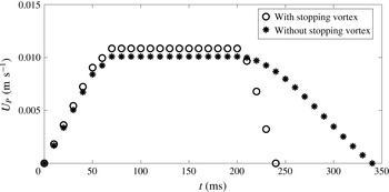
The velocity of the piston is obtained from the displacement of it, measured from the images taken using a high speed camera operating at 100 Hz. Figure 3(a) shows a typical variations of displacements of the piston with time. Piston motion can be divided in three parts; an initial acceleration of piston motion, followed by a region of nearby constant velocity (
 $U_{P}$
) and a deceleration part. The duration of deceleration time
 $t_{dec}$
, as shown in figure 3(b), is important in eliminating the stopping vortex.
Vortex ring with stopping vortex effects: a representative case for
 $Re_{exit}=3585$
and
 $I_{acc}/I_{T}=0.95$
. (a) Displacement and (b) velocity variation of the piston with time for generation and the corresponding (c) diameter and (d) translational velocity variation with time.

To characterize the jet, the exit velocity (
 $U_{s}$
) is defined as,
 $U_{s}=(U_{P}A_{P})/A_{0}$
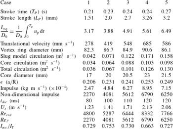
and the exit and vortex ring Reynolds numbers, tabulated in table 1, are defined respectively as,
 $Re_{exit}=(U_{s}D_{0})/\unicode[STIX]{x1D708}$
and
 $Re_{\unicode[STIX]{x1D6E4}}=\unicode[STIX]{x1D6E4}/\unicode[STIX]{x1D708}$
. Reynolds number, as defined in some earlier studies, as
 $Re=(L_{eq}D_{0})/(T_{P}\unicode[STIX]{x1D708})$
is also tabulated in table 1. The values of
 $\unicode[STIX]{x1D708}$
depend on the ambient conditions; the
 $\unicode[STIX]{x1D708}$
for cases 1 and 4 is
 $1.511\times 10^{-5}$
while that for cases 2, 3 and 5 is
 $1.568\times 10^{-5}$
.
Detailed parameters of the experimental cases discussed.

2.1 Flow visualization
To visualize the vortex ring, the driving chamber is filled with smoke. Minimizing the buoyancy effect is important for such vortex rings whose axis is horizontal and
 $Re$
is low. Else, the vortex ring either goes up or down due to buoyancy. This can easily be avoided in a vertically orientated set-up. However, the horizontal configuration ensures that the buoyancy effects does not influence the characteristics of the vortex ring. For flow visualization experiments, a continuous laser (1.2 W, 532 nm) is used for illuminating the flow field. A high speed camera of resolution
 $1028\times 1296$
pixels and frame rate of 2 kHz at full resolution is used for image capturing. The laser sheet is made to lie in a vertical plane passing through the nozzle diameter by using a cylindrical lens and images are captured at maximum 200 f.p.s.
2.2 Particle image velocimetry
Particle image velocimetry (PIV) technique is used to measure the velocity field of the vortex ring. A dual cavity, double-pulsed, Nd:YAG laser having energy of
 $300~\text{mJ}~\text{pulse}^{-1}$
, pulse width of 7 ns and repetition rate of 10 Hz is used for illuminating the flow field. The light is delivered from the laser head to the experimental zone by an articulated arm with a sheet forming optics. The sheet forming optics consists of two spherical lenses and a cylindrical lens. The thickness of the sheet is approximately 1 mm. The light sheet lies in the vertical diametral plane and parallel to the axis of the nozzle. A 12-bit, charge coupled device (CCD) camera of resolution
 $2048\times 2048$
pixels is used at 1 Hz frame rate in double frame mode. SAFEX fog fluid of density
 $1.353~\text{kg}~\text{m}^{-3}$
is used to generate the seeding particles. The diameter of the seeding particles is of the order of
 $1~\unicode[STIX]{x03BC}\text{m}$
. Note, as the camera frame rate used being 1 Hz, the images at higher time resolution are obtained by phase shifting the measurements with an appropriate delays in camera and laser with respect to piston motion in repeated experiments. The maximum error in the circulation of the fully formed vortex ring for repeated experiments is less than 2.3 %.
For tracing the flow field accurately, the particle response time should be faster than the smallest time scale of the flow. In order to estimate how well the seeding particles follow the fluid and their response to high velocity gradients, the Stokes number of the particle is calculated. Stokes number (
 $S_{tk}$
) can be defined as the ratio of the characteristic time of a particle (
 $\unicode[STIX]{x1D70F}_{p}$
) to the characteristic time of the flow (
 $\unicode[STIX]{x1D70F}_{f}$
). The particle relaxation time is given as
 $\unicode[STIX]{x1D70F}_{p}=(\unicode[STIX]{x1D70C}_{p}D_{p}^{2})/(18\unicode[STIX]{x1D707})$
where
 $\unicode[STIX]{x1D70C}_{p}$
is the particle density,
 $D_{p}$
is the diameter of the particle and
 $\unicode[STIX]{x1D707}$
is the fluid viscosity. The flow time scale is given by
 $\unicode[STIX]{x1D70F}_{f}=L_{f}/U_{f}$
where
 $L_{f}$
is characteristic length and
 $U_{f}$
is the characteristic velocity. The inner diameter of the nozzle is taken as the characteristic length and maximum velocity of the vortex ring, which it achieves after formation, is used as
 $U_{f}$
. The smaller the Stokes numbers, the better the tracing accuracy. When
 $S_{tk}\ll 0.1$
, then tracing accuracy errors are below 1 %. The Stokes number in the present experiments is of the order of
 $1.16\times 10^{-5}$
. Thus, the seeding particles can follow the velocity field of the flow accurately.
3 Role of stopping vortex and piston vortex
The effects of the stopping vortex and piston vortex are predominantly visible in the variation of diameter of a vortex ring with time. The evolution of a vortex ring diameter show a dip after reaching its maximum value which is an effect of stopping vortex and piston vortex as explained by Maxworthy (Reference Maxworthy1977), Didden (Reference Didden1979), Pullin (Reference Pullin1979), Blondeaux & De Bernardinis (Reference Blondeaux and De Bernardinis1983), Auerbach (Reference Auerbach1987), Irdmusa & Garris (Reference Irdmusa and Garris1987), Glezer (Reference Glezer1988), Auerbach (Reference Auerbach1991), Weigand & Gharib (Reference Weigand and Gharib1997), Allen & Auvity (Reference Allen and Auvity2002) and Cater et al. (Reference Cater, Soria and Lim2004). As can be seen in figure 1, the stopping vortex increases the translational velocity of a vortex ring and decreases the diameter before the primary vortex ring is free of its effects. Note that the stopping vortex itself moves in the reverse direction to the motion of the primary vortex ring and hence its effect is gradually diminished. Whereas, the piston vortex increases the diameter of the primary vortex ring causing the translational velocity to decrease followed by decrease in diameter as it moves into the vortex ring or ahead of its centre due to a leapfrog action (see figure 1 d).
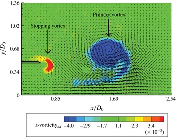
Figure 4 shows the PIV data of a vortex ring generated with a rapid deceleration of the piston (piston motion shown in figure 3
a,b) that resulted in creation of stopping vortex. The stopping vortex, as shown in figure 4, is of opposite vorticity to that of primary vortex ring and the circulation of the stopping vortex is approximately
 $11.6\,\%$
of the circulation of primary vortex. The diameter and velocity of a vortex ring with stopping vortex effects are shown in figures 3(c) and 3(d), respectively.
Vorticity of stopping vortex and primary vortex ring (
 $Re_{exit}=3585$
) at
 $t_{n}=tU_{s}/D_{0}=5.7$
.

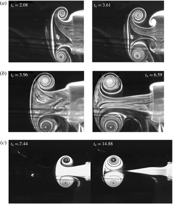
A series of flow visualization images of vortex rings under the effect of stopping vortex for
 $Re_{exit}=1780$
and 3660 are shown in figures 6(a) and 6(b) respectively. In figure 6(c), a vortex ring (
 $Re_{exit}=3304$
) is shown which is produced with large
 $t_{dec}$
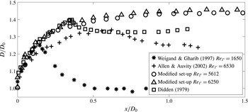
(see figure 5) and hence, it can be observed that there is no stopping vortex effect on this vortex ring. The stopping vortex is avoided by carefully choosing the piston time history which is stopped gradually. It can also be seen that there is no piston vortex present in the flow. To illustrate it further, the variation of vortex ring diameter with distance is plotted in figure 7 for cases with piston vortex (Allen & Auvity Reference Allen and Auvity2002), stopping vortex (Didden Reference Didden1979; Weigand & Gharib Reference Weigand and Gharib1997) and without stopping vortex. Parameters of the cases corresponding to present experiments are given in next section.
Velocity variation of piston for the cases with and without stopping vortex for
 $Re_{exit}=3585$
and 3304 respectively.

(a) Stopping vortex formation at high
 $I_{acc}/I_{T}\approx 0.92$
,
 $Re_{exit}=1780$
, (b) weak stopping vortex formation at
 $I_{acc}/I_{T}\approx 0.86$
,
 $Re_{exit}=3660$
and (c) no stopping vortex formation at
 $I_{acc}/I_{T}\approx 0.76$
,
 $Re_{exit}=3304$
.

It also shows the effect of piston vortex as observed by Allen & Auvity (Reference Allen and Auvity2002). The effect of the piston vortex, as discussed by Allen & Auvity (Reference Allen and Auvity2002), is avoided in this set-up by separating the piston from the nozzle. Thus the piston prevents scraping off the nozzle boundary layer which would have been present if the piston was inside the nozzle. All these improvements ensure the classical behaviour of the vortex ring (discussed later in reference to the theories) as expected and is referred to as a clean vortex ring.
3.1 Criterion for forming a clean vortex ring
To quantify the nature of deceleration that causes the stopping vortex ring formation or to find a criterion for the formation of the stopping vortex ring one needs to look into the cause of the formation of a stopping vortex. To quantify this, a set of experiments are carried out by measuring piston velocities and looking closely at the stopping vortex. In these visualization experiments, smoke is placed on the top half of the outer wall of the nozzle. When the piston decelerates, a reverse flow region appears in the inside wall of the nozzle. This causes entrained fluid motion from the outer side in the nozzle exit wall region that rolls up and forms a stopping vortex. Thus the stopping vortex formation process is expected to be a function of the rapidity of the piston stoppage, which can be quantified as fractional impulse imparted by the piston during the deceleration time. The ratio of acceleration impulse (
 $I_{acc}$
) calculated over
 $t_{acc}=T_{p}-t_{dec}$
and total impulse (
 $I_{T}=\int u^{2}\,\text{d}t$
) associated with the complete piston time history shows that if
 $I_{acc}/I_{T}<0.85$
the stopping vortex is either not formed or is very weak. This can be confirmed from figure 6, which shows the formation of a strong stopping vortex for
 $I_{acc}/I_{T}\approx 0.92$
, weak stopping vortex at
 $I_{acc}/I_{T}\approx 0.86$
and no stopping vortex at
 $I_{acc}/I_{T}\approx 0.76$
.
Comparison of vortex ring diameter with that of Didden (Reference Didden1979), Weigand & Gharib (Reference Weigand and Gharib1997) and Allen & Auvity (Reference Allen and Auvity2002).

4 Characteristics of a clean vortex ring
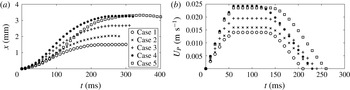
To discuss the detailed characteristics of a clean vortex ring, five cases are considered. The parameters for these cases are listed in table 1 and the corresponding piston displacements are shown in figure 8(a). The piston velocities are given in figure 8(b). For all these cases, stopping vortices do not form as
 $t_{dec}$
is large (
 $I_{acc}/I_{T}<0.75$
) compared to the case shown in figure 3(a,b).
(a) Displacement trajectory and (b) velocity variation of the piston for the five cases discussed.

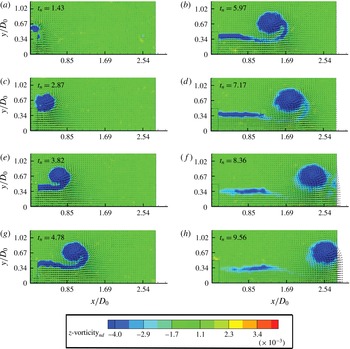
Superimposed velocity and vorticity fields, during evolution of a vortex ring, for different times are shown in figure 9 for case 2 (
 $Re_{exit}=5287$
). The vorticity shown is the non-dimensional azimuthal vorticity denoted as
 $z\text{-}\text{vorticity}_{nd}$
, scaled with
 $D_{0}/U_{s}$
. In all PIV figures, the origin is at the centre of the nozzle exit with
 $x$
-axis in the downstream direction and
 $y$
-axis in the radial direction. The nozzle is present up to
 $x/D_{0}=0.178$
, as shown in figure 9.
The vortex ring forms due to roll up of the wall shear layer at the exit of the nozzle, as seen in figure 9 for
 $t_{n}=tU_{s}/D_{0}<4.8$
. At this stage the vortex ring grows rapidly and the centre of the core of the vortex ring moves substantially in the radial direction. The radial motion diminishes beyond this time and the vortex ring moves with a self-induced axial velocity. As the stroke length is small, the vortex ring quickly detaches from the trailing jet. The jet shear layer strength diminishes due to two reasons, (i) the exit velocity diminishes quickly (by
 $t_{n}=8.4$
see figure 10) and the shear layer is no longer generated and (ii) entrainment of the shear layer vorticity to the main vortex ring core (see figure 9
 $t_{n}=7{-}10$
).
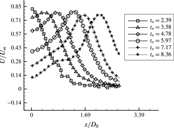
The axial velocity along the centreline at different time instances for case 2 is shown in figure 10. The axial location of the vortex core centre can be identified from the location of peak velocity. It also shows that during formation, the peak velocity increases as the strength of the vortex ring increases gradually during this time. Subsequently, the peak velocity remains nearly constant (as circulation at this stage remains nearly constant) except that it shows a dip during the pinching-off process (
 $t_{n}\simeq 9$
, figure 9) due to entrainment of low axial velocity fluid in the central part at this stage. Figure 10 also indicates the nature of centreline velocity at the exit (
 $x=0$
). Present experiments, having small stroke time, in comparison to experiments of Didden (Reference Didden1979) and the model of Krueger (Reference Krueger2005), show rapid decay of velocities at the exit (
 $x=0$
,
 $y=0$
) (see figure 10) with time for
 $t_{n}>5.8$
. Velocity at the exit increases with time in the data of Didden (Reference Didden1979) (see figure 4 of Krueger Reference Krueger2005).
Important parameters that characterize the dynamics of a vortex ring are the variations of core diameter, vortex bubble diameter, vortex ring diameter, vortex circulation, total circulation, impulse, energy and translational velocity with time. These quantities are measured or calculated and discussed in detail in this section for the clean vortex rings that are generated in the present experiments. All the parameters of cases 2, 3 and 5 could be found from PIV measurements carried out for these three cases.
 $Re_{\unicode[STIX]{x1D6E4}}$
presented in table 1 for these three cases are based on the experimental
 $\unicode[STIX]{x1D6E4}$
value of the vortex ring. For the other two cases, it is based on the
 $\unicode[STIX]{x1D6E4}$
estimated from slug flow circulation (Maxworthy Reference Maxworthy1972).
The evolution of the vortex ring for case 2.

Axial velocity variation with time for case 2.

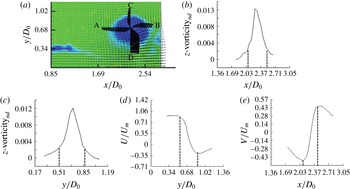
(a) The azimuthal vorticity and velocity vectors of the vortex ring, (b) the azimuthal vorticity distribution along the axial direction, (c) the azimuthal vorticity variation along the radial direction, (d) the velocity variation along the radial direction and (e) the velocity variation along the axial direction for case 2 at
 $t_{n}=10.14$
. The distance between the vertical dotted lines indicates the core diameter in (b)–(e).

4.1 Core diameter
In the literature, the core diameter of a vortex ring is defined in different ways such as that based on the vorticity distribution and the velocity distribution. It is an important parameter of the vortex ring and its accurate estimation is necessary for predicting the translational velocity theoretically. The method of calculating the core diameter (
 $d_{c}$
) in the present work is shown in figure 11. The azimuthal vorticity and the velocity vectors of the vortex ring are shown in figure 11(a) and the corresponding azimuthal vorticity distribution along the axial and the radial direction (along the lines AB and CD respectively) are shown in figures 11(b) and 11(c), respectively. The core diameter is calculated by two methods; (i) by taking the location where the vorticity drops to 10 % of its maximum value as given by Weigand & Gharib (Reference Weigand and Gharib1997) and (ii) by tracing the location of peak velocities as given by Arakeri et al. (Reference Arakeri, Das, Krothapalli and Lourenco2004). The average of the axial and radial core diameters is considered for both the methods. The vorticity distribution in figures 11(a) and 11(b) shows that the vorticity distribution in the vortex ring is nearly Gaussian. The corresponding velocity distribution along the radial and axial directions are shown in figures 11(d) and 11(e), respectively.
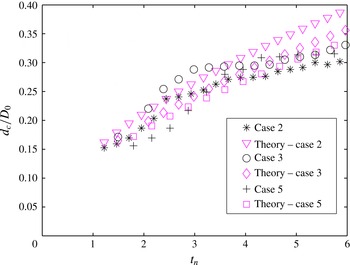
The non-dimensional core diameters of vortex rings for cases 2, 3 and 5 are shown in figure 12. Core diameter increases rapidly during the roll-up process when shear layer vorticity is fed into it. Its growth rate gradually decreases as the piston decelerates (
 $t_{n}>4.3$
) and reaches a nearly constant value after the vortex ring pinches off from the trailing jet shear layer (
 $t_{n}>7.5$
) and feeding of shear layer vorticity to the core stops. However, at larger time (not considered in the present study) due to viscous diffusion the
 $d_{c}$
should increase.
Defining core radius with different models for (a) case 2, (b) case 3 and (c) case 5.

As discussed above, core radius (
 $a$
) can be measured in different ways such as from the velocity variations or from the vorticity distribution. The core radius obtained as the distance between the points where the vorticity drops to 10 % of the maximum value of the vorticity is shown in figure 12 for the three cases. It can be seen that these values are comparable with the peak velocity based values (similar to Arakeri et al.
Reference Arakeri, Das, Krothapalli and Lourenco2004), as discussed above. Two other models are available for predicting core radius, Saffman (Reference Saffman1970) used
 $a=\sqrt{4\unicode[STIX]{x1D708}T}$
and Sullivan et al. (Reference Sullivan, Niemela, Hershberger, Bolster and Donnelly2008) considered total time elapsed in the calculation by adding the time of flight ‘
 $t$
’ to the stroke time. Figure 12 shows that both these models underpredict the core radius from the experimental values substantially. For comparison, the core radius calculated based on 50 % of the vorticity containing fluid is also plotted in figure 12. It is important to note that at higher
 $Re$
, the vorticity based core radius is more than the velocity based core radius. In all subsequent analyses the core radius
 $a$
is referred to as the core radius based on 90 % of vorticity.
Schematic showing that the fluid from the wall boundary layer forming the vortex ring core and annular shear layer zone.

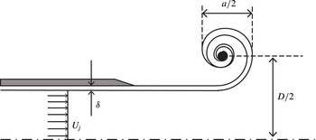
4.1.1 Model for core diameter during formation stage
In the literature, the model for the core radius and its comparison with the experimental value during the formation stage of the vortex ring is not adequate, as discussed above. However, with the assumption that during the formation stage the fluid from the boundary layer region enters the core, we attempt here to establish such a model. Saffman (Reference Saffman1978) and Pullin (Reference Pullin1979) found the self-similar nature of the initial roll-up process with the assumptions that the flow has just started and the vortex sheet at the nozzle exit behaves like a two-dimensional vortex sheet. Beyond this time, the core model is absent in the literature. The data that we have are for time periods beyond the self-similar roll-up process time. A simple model, with the assumption that the boundary layer vorticity flux from the nozzle inner wall forms the torus shaped vortex core and the annular shear layer in the trailing jet, is proposed here. The mass of boundary layer fluid ejected from the nozzle is equated with the volume of the core of the vortex ring and volume of the annular shear layer region of the trailing jet, as shown in figure 13. Flow from the central part of the pipe, having velocity (
 $U_{j}$
), forms the rest of the flow field along with the entrained fluid. This part is not directly involved in the present model. Entrainment of the ambient fluid into the core is also neglected in the model. The entrainment study of Dabiri & Gharib (Reference Dabiri and Gharib2004) shows that the volume of fluid entrained in the vortex bubble is 30 %–40 % of its volume for an isolated vortex ring with
 $L_{eq}/D_{0}=2{-}4$
. Thus, the volume of the entrained fluid into the vortex core alone during the formation stage is expected to be considerably lower and is neglected here. The balance equation can be written as,
 $$\begin{eqnarray}\int _{R_{0}-\unicode[STIX]{x1D6FF}}^{R_{0}}(2\unicode[STIX]{x03C0}tur\,\text{d}r)=(2\unicode[STIX]{x03C0}R_{0}\unicode[STIX]{x1D6FF}-\unicode[STIX]{x03C0}\unicode[STIX]{x1D6FF}^{2})U_{j}t+2\unicode[STIX]{x03C0}R\unicode[STIX]{x03C0}a^{2}.\end{eqnarray}$$
Here, the exit velocity at the central zone is
 $U_{j}$
, the vortex ring radius is
 $R$
, the boundary layer thickness is
 $\unicode[STIX]{x1D6FF}$
and
 $u$
is the velocity inside the boundary layer. All these quantities are functions of time. It will be shown in the next section that
 $D(t)$
follows the similarity law of Pullin (Reference Pullin1979) during the formation stage also, and hence
 $R=k_{s}t^{2/3}$
, where
 $k_{s}$
is the proportionality constant. According to Das (Reference Das1998),
 $\unicode[STIX]{x1D6FF}\approx 3.14\sqrt{\unicode[STIX]{x1D708}t}$
and from Shusser et al. (Reference Shusser, Gharib, Rosenfeld and Mohseni2002) and Krueger (Reference Krueger2005)
 $$\begin{eqnarray}U_{j}=U_{s}\left(1+8\sqrt{(\unicode[STIX]{x1D708}t)/(\unicode[STIX]{x03C0}D_{0}^{2})}\right).\end{eqnarray}$$
The velocity both in the central region and inside the boundary layer in the pipe can be determined exactly from Das & Arakeri (Reference Das and Arakeri1998), however for simplicity,
 $u$
is assumed to be a linear function of
 $r$
inside the boundary layer. Substituting these values in (4.1) one can easily find that,
 $$\begin{eqnarray}a=\sqrt{\frac{k_{1}^{2}U_{s}}{6\unicode[STIX]{x03C0}k_{s}}t^{4/3}+\frac{k_{1}^{2}k_{2}}{6\unicode[STIX]{x03C0}k_{s}}t^{11/6}}+\unicode[STIX]{x1D6FF}_{c}.\end{eqnarray}$$
Here,
 $K_{1}=3.14\sqrt{\unicode[STIX]{x1D708}}$
and
 $k_{2}=8U_{s}\sqrt{(\unicode[STIX]{x1D708})}/(\sqrt{\unicode[STIX]{x03C0}}D_{0})$
. The proportionality constant,
 $k_{s}$
is obtained in the next section for cases 2, 3 and 5 as 0.152, 0.164 and 0.146, respectively. The
 $\unicode[STIX]{x1D6FF}_{c}$
is the growth of the core due to viscous diffusion of the boundary layer fluid that rolls up and forms the core. Accurate estimation of the growth of the curved vortex sheet during unsteady roll up is not available. It is assumed to be the same as the Stokes first problem of impulsively started flow and hence,
 $\unicode[STIX]{x1D6FF}_{c}\approx 4\sqrt{\unicode[STIX]{x1D708}t}$
is used in present calculation.
Comparison of the predicted core diameter from the model with the experimental values during formation stage.

The values of
 $a$
during the formation stage i.e. for times less than 200 ms in the present study, are plotted from (4.3) and compared with the experimental data in figure 14. A reasonable comparison is achieved with this simple model until a time of approximately
 $t\simeq 150~\text{ms},t_{n}\simeq 5$
as after this time the piston motion decelerates (see figure 8).
4.2 Diameter of the vortex ring and vortex bubble
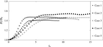
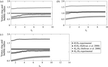
The diameter of the vortex ring is measured as the distance between the core centre observed in the cross-sectional plane view of the flow visualization images. The diameter of the vortex rings for all five cases are plotted in figure 15. Oscillations in the vortex ring diameter are due to the rotation of the core, which is not purely circular, as can be observed in figure 9. The vortex ring radius obtained from the flow visualization experiments is compared with the prediction from the theoretical model available. Sullivan et al. (Reference Sullivan, Niemela, Hershberger, Bolster and Donnelly2008) equated the volume swept out by the piston to the volume of fluid in the inner spheroid of the vortex ring and obtained the radius of the vortex ring as,
 $$\begin{eqnarray}R=\left(\frac{3R_{0}^{2}L}{4\unicode[STIX]{x1D6FE}}\right)^{1/3},\end{eqnarray}$$
where
 $\unicode[STIX]{x1D6FE}$
is the ratio of semi-minor to semi-major axes of the bubble and is taken as 0.6 by Sullivan et al. (Reference Sullivan, Niemela, Hershberger, Bolster and Donnelly2008).
Variation of vortex ring diameter with time.

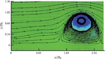
The vortex atmosphere seals the vortex ring from oncoming flow and the fluid inside the vortex bubble is isolated from the rest of the jet. The bubble radius is calculated from the PIV experiments (figure 16) and is taken as the reference for the comparison of the theoretical model available for the estimation of the bubble radius. The model that is available in the literature for determining the vortex bubble radius is again by Sullivan et al. (Reference Sullivan, Niemela, Hershberger, Bolster and Donnelly2008) who used mass and momentum balance to reach at the following result for the bubble radius,
 $$\begin{eqnarray}R_{b}=\left(\frac{9\unicode[STIX]{x03C0}R_{0}^{2}L}{4\unicode[STIX]{x1D6FE}^{2}\left(\ln {\displaystyle \frac{8R}{a}}-0.558\right)(1+k)}\right).\end{eqnarray}$$
Here,
 $k$
is the Bessel added mass factor which is taken as 0.65 (Sullivan et al.
Reference Sullivan, Niemela, Hershberger, Bolster and Donnelly2008).
Bubble streamlines used to calculate bubble radius for case 3 at
 $t_{n}=10.14$
.

The above mentioned models for the three cases discussed here are shown in figures 17(a), 17(b) and 17(c), respectively. The vortex ring radius and the bubble radius (figure 17 a–c) as calculated by the models by Sullivan et al. (Reference Sullivan, Niemela, Hershberger, Bolster and Donnelly2008) are high compared to the experimentally observed vortex ring radius and the bubble radius. The reason for such a huge discrepancy is probably due to the inadequate knowledge of the entrainment effect, which is not included in the model. Also, the model is unable to account for the trailing jet fluid accurately. These models balance either exit mass or momentum of the fluid that is coming out of the nozzle with that of vortex bubble. Actually, some part of the jet fluid goes into the vortex atmosphere and some part of the ambient fluid enters the core, which are not accounted for in the model.
The vortex ring radius is also predictable during the initial roll-up process from the similarity solution of Saffman (Reference Saffman1978) and Pullin (Reference Pullin1979). During the initial spiralling process, substantial radial movement of the spiral centre is observed. However, once the radial velocity diminishes, the diameter does not change with time, unlike the core diameter. This can be observed from figures 12 and 15 where the vortex ring diameter at approximately
 $t_{n}=5.8$
becomes constant whereas the core diameter continues to grow beyond this time. Thus, it is expected that the core dynamics is more complex compared to the inviscid roll-up process that determines the ring diameter. The data up to
 $t_{n}=4$
for all the cases are fitted as
 $D\sim t^{q}$
and it is found that
 $q$
varies from 0.6 to 0.7. Thus the similarity model for which
 $q=2/3$
predicts the experimentally obtained
 $D$
values reasonably well during the formation stage. The proportionality constant (
 $k_{s}$
) from the experimental fit data for case 2, case 3 and case 5 are 0.152, 0.164 and 0.146, respectively.
Vortex ring radius and bubble radius obtained from different models for (a) case 2, (b) case 3 and (c) case 5.

4.3 Impulse
The impulse associated with the formation of a vortex ring is the external force that is applied to the slug of fluid that forms the vortex ring and is defined by Lamb (Reference Lamb1932) (Akhmetov Reference Akhmetov2008). The impulse (
 $P$
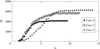
) is calculated using (1.4) and the non-dimensional impulse (
 $P_{n}$
), shown in figure 18, is calculated as,
 $$\begin{eqnarray}P_{n}=\frac{P}{\unicode[STIX]{x1D70C}\unicode[STIX]{x03C0}R^{2}\unicode[STIX]{x1D708}}.\end{eqnarray}$$
Note that
 $P_{n}=Re_{\unicode[STIX]{x1D6E4}}$
, a local Reynolds number of the vortex ring. It is also noted that the time when
 $Re_{\unicode[STIX]{x1D6E4}}$
becomes constant is the time when the vortex ring is fully formed.
Variation of non-dimensional impulse with non-dimensional time.

4.4 Circulation
Circulation
 $\unicode[STIX]{x1D6E4}$
is a measure of the strength of the vortex ring and is a very important parameter to describe the dynamics. Exact values of the core radius,
 $a$
(
 $=d_{c}/2$
) and
 $\unicode[STIX]{x1D6E4}$
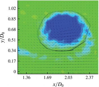
are required to find the theoretical value of translational velocity of the vortex ring and can be easily obtained from PIV measurements. A polygon (shown in figure 19) encircling the core region is used to calculate
 $\unicode[STIX]{x1D6E4}$
and is denoted as the vortex circulation. The polygon is chosen manually such that the jet shear layer circulation is eliminated in the estimation of core circulation. The total circulation,
 $\unicode[STIX]{x1D6E4}_{T}$
is calculated using the velocity along the centreline. Variations of
 $\unicode[STIX]{x1D6E4}$
and
 $\unicode[STIX]{x1D6E4}_{T}$
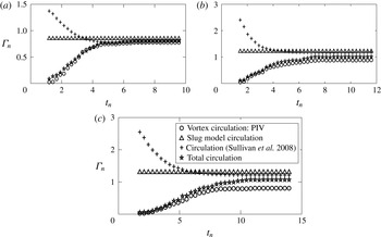
are shown in figure 20 for three of the cases for which PIV measurements are carried out. Both
 $\unicode[STIX]{x1D6E4}$
and
 $\unicode[STIX]{x1D6E4}_{T}$
are non-dimensionalized by
 $U_{s}D_{0}$
(Weigand & Gharib Reference Weigand and Gharib1997).
 $\unicode[STIX]{x1D6E4}$
increases with time during the formation stage and gradually becomes constant as the feeding of shear layer vorticity to the core stops.
 $\unicode[STIX]{x1D6E4}$
does not change after the vortex ring pinches off from the jet shear layer and
 $\unicode[STIX]{x1D6E4}_{T}$
becomes constant when the flow at the nozzle exit stops. As Reynolds number increases, the difference between
 $\unicode[STIX]{x1D6E4}$
and
 $\unicode[STIX]{x1D6E4}_{T}$
increases, which is an effect of the strength of the shear layer vorticity. To establish the initial roll-up process, the value of
 $\unicode[STIX]{x1D6E4}$
is fitted with time and it is observed that the variation of
 $\unicode[STIX]{x1D6E4}$
does not follow
 $\unicode[STIX]{x1D6E4}\sim t^{1/3}$
, as given by Pullin (Reference Pullin1979), during the formation process beyond the time of initial spiralling of the vortex sheet.
The polygon used for the calculation of circulation,
 $\unicode[STIX]{x1D6E4}$
of the vortex ring core.

Variation of circulation with time for (a) case 2, (b) case 3 and (c) case 5.

However, beyond the self-similar roll-up time, the data show rapid augmentation of
 $\unicode[STIX]{x1D6E4}$
. This is clear from the nature of the variation of
 $\unicode[STIX]{x1D6E4}$
with time, obtained from experiments and shown in figure 20. The nature of the curve at the formation stage in figure 20 is similar to that obtained by Dabiri & Gharib (Reference Dabiri and Gharib2004). Figure 20 also shows that
 $\unicode[STIX]{x1D6E4}_{T}$
is marginally greater than
 $\unicode[STIX]{x1D6E4}$
during the initial roll-up process. At the spiralling stage, the shear layer
 $\unicode[STIX]{x1D6E4}$
is nearly absent as the trailing jet is not established and the contribution of circulation due to overpressure
 $\unicode[STIX]{x1D6E4}_{p}$
to
 $\unicode[STIX]{x1D6E4}_{T}$
, as discussed by Krueger (Reference Krueger2005), plays a role. The equation for variation of
 $\unicode[STIX]{x1D6E4}$
with time can be written as,
 $$\begin{eqnarray}\frac{\text{d}\unicode[STIX]{x1D6E4}}{\text{d}t}=\int _{0}^{\infty }u\unicode[STIX]{x1D714}_{\unicode[STIX]{x1D703}}\,\text{d}y=\int _{0}^{\infty }\left(\frac{\text{d}v}{\text{d}x}-\frac{\text{d}u}{\text{d}y}\right)u\,\text{d}y.\end{eqnarray}$$
On the right-hand side of (4.7), the first term is the variation of
 $\unicode[STIX]{x1D6E4}_{p}$
and the second term is the variation of slug model
 $\unicode[STIX]{x1D6E4}_{s}$
with time. These terms are directly calculated from the measured PIV data and their sum is compared with the variation of
 $\unicode[STIX]{x1D6E4}$
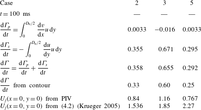
obtained through the integration of velocity around a contour shown in figure 19 and are tabulated in table 2 for
 $t=100~\text{ms}$
. Estimation from the PIV data show that the term for overpressure is small for all these cases. The value of
 $\text{d}\unicode[STIX]{x1D6E4}/\text{d}t$
(sum of both the terms) is close to the corresponding
 $\text{d}\unicode[STIX]{x1D6E4}/\text{d}t$
values estimated from contours. Thus it gives us a direct measurement and shows that contribution of overpressure circulation is less than 2.5 % in the present experiments.
Comparison of theoretical
 $\text{d}\unicode[STIX]{x1D6E4}/\text{d}t$
(
 $\text{m}^{2}~\text{s}^{-2}$
) and
 $U_{j}$
(
 $\text{m}~\text{s}^{-1}$
) with experiments.

A model of circulation can easily be written neglecting the overpressure term from (4.7) as,
 $$\begin{eqnarray}\frac{\text{d}\unicode[STIX]{x1D6E4}}{\text{d}t}=\frac{U_{j}^{2}}{2}.\end{eqnarray}$$
Again writing
 $U_{j}$
from (4.2),
 $\unicode[STIX]{x1D6E4}$
can be written as,
 $$\begin{eqnarray}\unicode[STIX]{x1D6E4}={\textstyle \frac{1}{2}}U_{j}^{2}t+{\textstyle \frac{1}{4}}k_{2}^{2}t^{2}+{\textstyle \frac{2}{3}}U_{j}k_{2}t^{3/2}.\end{eqnarray}$$
The nature of the variation of
 $\unicode[STIX]{x1D6E4}$
with time does indicate the above trend during the formation stage. However, due to overprediction of
 $U_{j}$
in the model given in (4.2), the circulation prediction from (4.9) is not accurate. It overpredicts the circulation considerably. Experimental
 $U_{j}$
values obtained at
 $t=100~\text{ms}$
in PIV shows 37 %–83 % difference with that obtained from (4.2) (table 2).
The vortex ring circulation and total circulation measured from the PIV measurements after it is fully formed are also compared with other available theoretical models. Models that are available in the literature for determining the circulation of a vortex ring are the slug model and the impulse based model. The slug model given by Maxworthy (Reference Maxworthy1977) and Didden (Reference Didden1979) assumes that the vortex ring is formed from a cylindrical ‘slug’ of fluid of length
 $L$
ejected from the exit of the nozzle over a stroke time
 $T$
. The slug model gives an expression for circulation as (see (1.7)),
 $\unicode[STIX]{x1D6E4}_{S}=L^{2}/2T$
. Sullivan et al. (Reference Sullivan, Niemela, Hershberger, Bolster and Donnelly2008) assumed that the impulse of the ring is close to the momentum given to the fluid by the piston and gives the expression for the circulation as,
 $$\begin{eqnarray}\unicode[STIX]{x1D6E4}=\frac{R_{0}^{2}L^{2}}{R^{2}T},\end{eqnarray}$$
where
 $L$
is the equivalent stroke length,
 $R_{0}$
is the nozzle exit radius,
 $R$
is the vortex ring radius and
 $T$
is the stroke time.
The circulation values obtained from the above mentioned models (valid for a fully formed vortex ring) are compared for the cases 2, 3 and 5 and shown in figures 20(a), 20(b) and 20(c), respectively. From figure 20(a–c), it can be observed that both the slug model and the model by Sullivan et al. (Reference Sullivan, Niemela, Hershberger, Bolster and Donnelly2008) overpredict the circulation value. However, the model by Sullivan et al. (Reference Sullivan, Niemela, Hershberger, Bolster and Donnelly2008) predicts it better than the slug model. From these figures, it can be observed that the difference with the experimental data increases with the increase of Reynolds number after the vortex ring has fully formed. This is due to the trailing jet circulation which is not accounted in these models. From the above discussion it is clear that a better model that includes the effects of the jet circulation and its entrainment into the vortex ring is required. Time resolved velocity measurements with high spatial accuracy are necessary to arrive at a better model for circulation.
4.5 Translational velocity of the vortex ring
The translational velocity,
 $V$
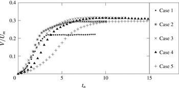
, of the vortex ring is calculated by tracing the core centre of the vortex ring at 200 Hz and is shown in figure 21 for all five cases considered. Five point central differencing is used to calculate the velocity from the measured positions. The translational velocity does not show any stopping vortex or piston vortex effects and gradually increases to fully formed
 $V$
for all the cases.
Variation of translational velocity of vortex ring with time.

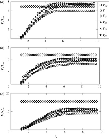
Comparison of predicted translational velocity from different models with experiments for (a) case 2, (b) case 3 and (c) case 5.

We could obtain salient parameters of the vortex ring such as
 $D$
,
 $d_{c}$
and
 $\unicode[STIX]{x1D6E4}$
through high speed visualization and PIV measurements. Various existing theoretical models and empirical relations are available in the literature for predicting different parameters of a vortex ring, barring translational velocity, and have already been discussed. The limitations of the existing theoretical models that predict some of these parameters, such as core diameter, ring diameter and circulation, have been illustrated. Comparison of the experimentally obtained
 $V$
with the theoretical models are discussed in this section to illustrate their validity. Such detailed comparisons are not available in the literature and are essential in view of the several theoretical and empirical results available in the vast literature on vortex ring studies. Surprisingly, very few efforts exist on the comparison of theory with experiments when the question of translational velocity is addressed, particularly during the formation stage. The reason could be the effects of the piston vortex and stopping vortex. In figure 22(a), (b) and (c), different available theoretical models of translational velocity are compared with the experimentally obtained
 $V$
for case 2, case 3 and case 5, respectively. The details of the theoretical models considered can be broadly classified into two categories, (i) circulation based inviscid and viscous models and (ii) energy and impulse based models.
When the core radius is much smaller than the vortex ring radius (
 $a\ll R$
), it is shown by Saffman (Reference Saffman1970) that the vortex ring moves forward with velocity,
 $V$
given by (1.3). The translational velocity, given by Saffman (Reference Saffman1970), can alternatively be written with the slug model circulation, based on the stroke length (§ 1.2) and the stroke time of the piston (table 1), (Maxworthy Reference Maxworthy1977; Didden Reference Didden1979) as,
 $$\begin{eqnarray}V_{S}=\frac{L_{eq}^{2}}{8\unicode[STIX]{x03C0}RT}\left(\ln \frac{8R}{a}-\unicode[STIX]{x1D6FD}\right),\end{eqnarray}$$
where
 $L_{eq}$
is the equivalent stroke length of the piston, as defined in § 1.2. It is evident from the properties of vortex rings discussed in § 4.1 that ‘
 $a$
’ as
 $\sqrt{4\unicode[STIX]{x1D708}T}$
(Saffman Reference Saffman1970) or
 $\sqrt{4\unicode[STIX]{x1D708}T+t}$
(Sullivan et al.
Reference Sullivan, Niemela, Hershberger, Bolster and Donnelly2008) underpredict the core radius and hence are not shown in figure 22(a–c). Fukumoto & Moffatt (Reference Fukumoto and Moffatt2000) accounted for the viscous effects on the motion of the vortex ring in a viscous fluid and modified the relation of Saffman (Reference Saffman1970) as,
 $$\begin{eqnarray}V_{fm}=\frac{\unicode[STIX]{x1D6E4}}{4\unicode[STIX]{x03C0}R}\left\{\ln \frac{8R}{\sqrt{4\unicode[STIX]{x1D708}T}}-0.558-3.6716\frac{\unicode[STIX]{x1D708}t}{R^{2}}\right\}.\end{eqnarray}$$
The term (
 $(3.6716\unicode[STIX]{x1D708}t)/R^{2}$
) is the viscous effect term and the negative sign indicates the slowing of the vortex ring due to viscosity.
 $V$
calculated from Saffman’s (1970) model and the model of Fukumoto & Moffatt (Reference Fukumoto and Moffatt2000) should differ marginally as the contribution of viscous term (
 $(3.6716\unicode[STIX]{x1D708}t)/R^{2}$
) is usually small unless we are looking for the
 $V$
at a much later time, when viscous diffusion becomes important. However, figure 22(a–c) show considerable differences between the two models. One can see from these figures that formula given by Fukumoto & Moffatt (Reference Fukumoto and Moffatt2000) predicts the velocity to be closer to the experimentally observed
 $V_{exp}$
compared to (1.3). The implication of this observation could be misleading as it indicates a substantial viscous effect at this stage. The actual reason for this is different. In (1.3),
 $a$
and
 $\unicode[STIX]{x1D6E4}$
are taken from experiments whereas in (4.12), a wrong and smaller
 $a=\sqrt{4\unicode[STIX]{x1D708}T}$
is used and hence the velocity predicted is higher. Tung & Ting (Reference Tung and Ting1967) provided a formula for the translational velocity of a finite core viscous vortex ring as,
 $$\begin{eqnarray}V_{TT}=\frac{\unicode[STIX]{x1D6E4}}{4\unicode[STIX]{x03C0}R}\left(\ln \frac{8R}{\sqrt{4\unicode[STIX]{x1D708}t}}-0.688\right),\end{eqnarray}$$
where the core radius is taken as
 $\sqrt{4\unicode[STIX]{x1D708}t}$
. Equation (4.13) overpredicts
 $V_{exp}$
as the core radius taken is smaller than the actual
 $a$
. However, if the experimental
 $a$
is substituted into (4.13), it underpredicts the experimental value (not shown here). This observation probably reopens the question of what should be the value of the constants in (4.12) and (4.13).
Another class of formulas that are derived for predicting translational velocity is based on energy and impulse of the vortex ring. Shusser & Gharib (Reference Shusser and Gharib2000) gave an expression for the translational velocity of thick vortex rings using impulse and the vortex circulation as,
 $$\begin{eqnarray}V_{sg}=0.5352\sqrt{\frac{\unicode[STIX]{x1D70C}\unicode[STIX]{x1D6E4}^{3}}{\unicode[STIX]{x03C0}P}}.\end{eqnarray}$$
Sullivan et al. (Reference Sullivan, Niemela, Hershberger, Bolster and Donnelly2008) replaced slug model circulation in the expression given by Shusser & Gharib (Reference Shusser and Gharib2000) and modified the translational velocity as,
 $$\begin{eqnarray}V_{sg1}=0.5352\frac{\unicode[STIX]{x1D6E4}_{s}}{\unicode[STIX]{x03C0}R_{0}},\end{eqnarray}$$
where
 $\unicode[STIX]{x1D6E4}_{s}$
is slug model circulation, calculated based on
 $L_{eq}$
. In comparison with the present data, only
 $V_{sg1}$
is plotted as
 $V_{sg}$
underpredicts the translational velocity substantially. According to Sullivan et al. (Reference Sullivan, Niemela, Hershberger, Bolster and Donnelly2008), the kinetic energy of a vortex ring with
 $R\gg a$
(
 $a$
obtained from PIV experiment is used here) is given by equation 1.2. Hamilton’s equation relates the energy and the impulse (given in (1.4)) of the vortex ring to the translational velocity as,
 $$\begin{eqnarray}V_{g1}=\frac{\unicode[STIX]{x2202}E}{\unicode[STIX]{x2202}P}.\end{eqnarray}$$
The model of Sullivan et al. (Reference Sullivan, Niemela, Hershberger, Bolster and Donnelly2008) is the simplified model of Fraenkel (Reference Fraenkel1972), who derived the second-order formulae for the impulse and energy of vortex rings with finite but small values of
 $\unicode[STIX]{x1D700}$
(
 $=a/R$
) as,
 $$\begin{eqnarray}\displaystyle & \displaystyle E_{\unicode[STIX]{x1D700}}=\frac{1}{2}\unicode[STIX]{x1D70C}R\unicode[STIX]{x1D6E4}^{2}\left(\ln \frac{8}{\unicode[STIX]{x1D700}}-\frac{7}{4}+\frac{3}{16}\unicode[STIX]{x1D700}^{2}\ln \frac{8}{\unicode[STIX]{x1D700}}\right) & \displaystyle\end{eqnarray}$$
 $$\begin{eqnarray}\displaystyle & \displaystyle P_{\unicode[STIX]{x1D700}}=\unicode[STIX]{x1D70C}\unicode[STIX]{x1D6E4}\unicode[STIX]{x03C0}R^{2}\left(1+\frac{3}{4}\unicode[STIX]{x1D700}^{2}\right). & \displaystyle\end{eqnarray}$$
Using Hamilton’s equation, the translational velocity is calculated as,
 $$\begin{eqnarray}V_{g2}=\frac{\unicode[STIX]{x2202}E_{\unicode[STIX]{x1D700}}}{\unicode[STIX]{x2202}P_{\unicode[STIX]{x1D700}}}.\end{eqnarray}$$
The core radius used for calculating energy and impulse is the one obtained from PIV experiments. In the above two models, when the velocity is recalculated by replacing the core radius based on
 $a=\sqrt{4\unicode[STIX]{x1D708}T}$
or
 $a=\sqrt{4\unicode[STIX]{x1D708}(T+t)}$
, both models overpredict the translational velocity as the core radius is underpredicted using these relations (see figure 12).
It is also observed that the model of Tung & Ting (Reference Tung and Ting1967) calculates
 $V$
more accurately than the model of Saffman (Reference Saffman1970) (see figure 22
a–c). For all the cases, it can be seen that
 $V$
calculated from the model of Fraenkel (Reference Fraenkel1972), matches the experimentally measured
 $V$
to a good extent.
Other than the model of Fraenkel (Reference Fraenkel1972), figure 22(a–c) show that at large
 $t_{n}$
, the results from the models of Tung & Ting (Reference Tung and Ting1967) and Fukumoto & Moffatt (Reference Fukumoto and Moffatt2000) match with
 $V_{exp}$
reasonably well, as at this stage the vortex ring has a finite core and viscous effects become gradually important. During the initial formation stage, the model of Tung & Ting (Reference Tung and Ting1967) appears best for all Reynolds numbers. The model of Fukumoto & Moffatt (Reference Fukumoto and Moffatt2000) also appears to predict the translational velocity at this stage. However, the models of Tung & Ting (Reference Tung and Ting1967) and Fukumoto & Moffatt (Reference Fukumoto and Moffatt2000) suffer from the drawback of using an underpredicted core diameter and overpredicted circulation. To predict the translational velocity at this stage one needs to consider the dynamics of a spiralling shear layer and formation of the core with Stokes layer type viscous diffusion of the shear layer fluid, as discussed in § 4.1.1 (4.3) which is beyond the scope of this work.
From the detailed comparisons of the data presented here and those of earlier studies, clear variations are observed in different quantities that are modelled. Although a great deal of experimental data are necessary to find empirical correlations for these quantities, the present work highlights the limitations and validity of existing models with the measured quantities through a novel experimental arrangement. In summary, the following important characteristics are noted for a vortex ring. The measured values of the core radius are substantially different from the values obtained in theoretical models, used by different investigators. The estimation of the core radius requires detailed velocity field measurements, which are limited in the literature, and the models used to determine its value always underpredict it. Similarly, the vortex ring radius and circulation differ from the available models considerably and this indicates the need of better models. The core radius and circulation, obtained from the respective models, are used in the models for the translational velocity (see (1.3), (4.12) and (4.13)) and it appears that the error due to using the underpredicted core radius and overpredicted circulation have resulted in the constant values of translational velocity. However, the present study clearly indicates that these constants need to be corrected when one uses the correct core radius and circulation values. The ratio of translational velocity of a fully formed vortex ring and exit velocity does not have a constant value and varies from 0.46 to 0.65 in the different cases considered here, as can be obtained from table 1. This is consistent with the observations of previous investigators (Sullivan et al. Reference Sullivan, Niemela, Hershberger, Bolster and Donnelly2008). However, in the present observations, we could identify the best model for prediction of the translational velocity as the model of Fraenkel (Reference Fraenkel1972). A detailed study of the effects of Reynolds number and the slowing down of motion can be obtained in the future.
5 Conclusions
Dynamics of the vortex ring is revisited experimentally with a novel experimental arrangement. The experimental arrangement could successfully eliminate the piston vortex, stopping vortex and orifice generated vortices. Observing the absence of the dip in diameter after the implementation of the modifications in the set-up and experimental procedure, it can be said that the effects of the stopping vortex and piston vortex are eliminated. A criterion based on the impulse associated with the deceleration of the piston that drives the flow is given for the elimination of the stopping vortex. It is observed that if the impulse associated with the deceleration of the piston is less than 15 % of the total impulse imparted by the piston, a stopping vortex forms. The strength of the stopping vortex depends on the rapidity of the piston deceleration.
Formation and propagation characteristics of the clean vortex ring are discussed in detail with reference to earlier studies. The vorticity distribution in the core of the vortex ring, measured using PIV, is found to be nearly Gaussian. From figure 20(a–c), it can be observed that the slug model overpredicts the circulation and the circulation given by Sullivan et al. (Reference Sullivan, Niemela, Hershberger, Bolster and Donnelly2008) matches well with the total circulation after the ring has fully formed at low Reynolds numbers. At high Reynolds numbers, the model does not account for the trailing jet circulation and fails to predict its value. Also the model of Krueger (Reference Krueger2005) fails to predict the circulation during the formation stage due to overprediction of exit velocity in their model. The vortex ring radius and the bubble radius (figure 17 a–c) as calculated by Sullivan et al. (Reference Sullivan, Niemela, Hershberger, Bolster and Donnelly2008) are approximately twice the experimentally observed vortex ring radius and bubble radius. This is because these models balance either exit mass or momentum of the fluid that is coming out of the nozzle with that of vortex bubble. Actually, some part of this fluid goes into the vortex atmosphere and some part of the ambient fluid enters the core, which are not accounted for in the model. However, in the initial stage, the growth of the diameter is found to be self-similar, as predicted by the similarity solution of Saffman (Reference Saffman1978) and Pullin (Reference Pullin1979). The core radius is an important parameter for the prediction of translational velocity of a vortex ring and it is found that core radius based on 90 % vorticity almost matches the core radius based on the velocity peak. Core radius calculated based on stroke time is much lower than the experimental value. A new model for the core radius is obtained based on the assumption that the boundary layer region fluid from the pipe forms the core and the shear layer. The model predicts the core radius during the formation stage quite satisfactorily. Several models that exist for prediction of translational velocity are compared with the measured values. The translational velocity models can be largely categorized as circulation based models and energy impulse based models. The circulation based models are either inviscid or viscous with a thin or thick core. However, because of inaccurate modelling of the core and circulation, most of these models fail to predict the translational velocities. Based on the experimentally measured core radius and vortex ring circulation, Fraenkel’s (1972) finite core model is found to be the most accurate for predicting the translational velocity of a vortex ring.
Acknowledgements
The authors would like to acknowledge Mr A. Kr. Gupta, C. L. Dora, S. Kr. Ghosh and K. K. Bharadwaj for help during flow visualization and PIV measurements. We also acknowledge the support of the CARE programme of IIT Kanpur.