1 Introduction
Magnetic filaments are spontaneously generated by the growth of the Weibel, or filamentation, instability. This instability is triggered when two relativistic plasma shells cross each other (Huntington et al. Reference Huntington, Fiuza, Ross, Zylstra, Drake, Froula, Gregori, Kugland, Kuranz and Levy2015). It has been invoked for intergalactic magnetic field generation (Schlickeiser & Shukla Reference Schlickeiser and Shukla2003), inertial confinement fusion (Silva et al. Reference Silva, Fonseca, Tonge, Mori and Dawson2002; Deutsch et al. Reference Deutsch, Bret, Firpo and Fromy2005), or collisionless shock physics (Medvedev & Loeb Reference Medvedev and Loeb1999; Fiuza et al. Reference Fiuza, Fonseca, Tonge, Mori and Silva2012; Bret et al. Reference Bret, Stockem, Fiúza, Ruyer, Gremillet, Narayan and Silva2013). Regarding collisionless shocks, it has been known for a long time that they are capable of accelerating particles (Blandford & Eichler Reference Blandford and Eichler1987); for a particle to receive energy, and keep it, the medium has to be collisionless. As such, it is believed that they may play a key role in the generation of high-energy cosmic rays, or gamma-ray bursts (Vietri, De Marco & Guetta Reference Vietri, De Marco and Guetta2003; Piran Reference Piran2004).
During the last decade or so, the physics of collisionless shocks has undergone renewed interest, as it has become possible to study them in detail through large-scale particle-in-cell simulations (Silva et al. Reference Silva, Fonseca, Tonge, Dawson, Mori and Medvedev2003; Spitkovsky Reference Spitkovsky, Bulik, Rudak and Madejski2005; Niemiec et al. Reference Niemiec, Pohl, Bret and Wieland2012). On the theory side, one of the problems currently being solved has to do with the very formation of such shocks. Concerning fluid shocks, it is known that they can arise from the steepening of a large-amplitude sound wave, or from the collision of two media, with a collision speed faster than the speed of sound in one of them (Zel’dovich & Raizer Reference Zel’dovich and Raizer2002). The formation process in the collisionless case is more involved because such shocks occur in collisionless plasmas. In these kinds of settings, where the collision frequency is virtually zero, a shock has to be mediated by collective plasma interactions (Sagdeev Reference Sagdeev1966).
As electromagnetic objects, collisionless shocks display far more variety than fluid shocks. They can be electrostatic or electromagnetic (Weibel) (Sarri et al. Reference Sarri, Dieckmann, Kourakis and Borghesi2011; Dieckmann et al. Reference Dieckmann, Sarri, Doria, Ahmed and Borghesi2014; Stockem et al. Reference Stockem, Fiuza, Bret, Fonseca and Silva2014), form in pairs or electron/ion plasmas (Bret et al. Reference Bret, Stockem, Fiúza, Ruyer, Gremillet, Narayan and Silva2013, Reference Bret, Stockem, Narayan and Silva2014; Novo et al. Reference Novo, Bret, Fonseca and Silva2015), and on the top of these dichotomies, be influenced by the strength of an external magnetic field and its orientation (Treumann Reference Treumann2009; Marcowith et al. Reference Marcowith, Bret, Bykov, Dieckman, Drury, Lembège, Lemoine, Morlino, Murphy and Pelletier2016).
Among the different kinds of collisionless shocks, an interesting sub-class is formed by the so-called ‘Weibel shocks’. When two collisionless plasma shells run into each other, the overlapping region turns unstable. If the encounter occurs at relativistic velocity, the dominant instability is the Weibel one (Bret & Deutsch Reference Bret and Deutsch2005; Bret et al. Reference Bret, Gremillet, Bénisti and Lefebvre2008; Bret, Gremillet & Dieckmann Reference Bret, Gremillet and Dieckmann2010). This instability grows magnetic filaments which can block the incoming flow, initiating the shock formation (Bret et al. Reference Bret, Stockem, Fiúza, Ruyer, Gremillet, Narayan and Silva2013, Reference Bret, Stockem, Narayan and Silva2014; Novo et al. Reference Novo, Bret, Fonseca and Silva2015).
Note that at the very beginning of the shock formation process, the counter-streaming plasmas cross each other, triggering the Weibel instability. At this stage, magnetic filaments are under formation, and particles are not stopped. Then the Weibel instability reaches saturation and the filaments are fully formed, and may stop the particles arriving at later times. The flow stopped by the filaments is not the flow that formed them.
It is clear that in the shock setting, once the filaments have stopped a number of particles, these may perturb the filaments and break them. Yet, it has been found that the resulting field configuration is at least as efficient as were the filaments to stop the flow (Bret et al. Reference Bret, Stockem, Narayan and Silva2014; Novo et al. Reference Novo, Bret, Fonseca and Silva2015). In order to know whether a shock will start forming after the saturation of the Weibel instability or not, the key question is therefore: at saturation time, are the filaments able to block the incoming particles?
For the case where there is no external magnetic field, the conditions upon which the flow is blocked can be derived from the analysis of the motion of charged particles in the Weibel magnetic filaments (Bret Reference Bret2015). Yet, many astrophysical settings are magnetized. If two plasma shells interact over an external, flow-aligned, magnetic field
 $\boldsymbol{B}_{0}$
, the Weibel instability still grows while the field is not too strong (Godfrey, Shanahan & Thode Reference Godfrey, Shanahan and Thode1975; Bret, Dieckmann & Deutsch Reference Bret, Dieckmann and Deutsch2006). Here, the resulting magnetic filaments supposed to block the incoming flow for the shock to form will be superimposed over the external
 $\boldsymbol{B}_{0}$
. The goal of this article is therefore to study this problem: what is the trajectory of charged particles within magnetic filaments and an external
 $\boldsymbol{B}_{0}$
?
2 Model considered
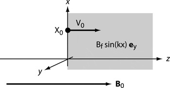
We therefore consider the set-up pictured in figure 1. The half-space
 $z>0$
is filled with the magnetic filaments
 $\boldsymbol{B}_{f}=B_{f}\sin kx\boldsymbol{e}_{y}$
, where
 $k^{-1}$
is therefore the coherence length of the magnetic field. A static, homogeneous, external magnetic field
 $\boldsymbol{B}_{0}=B_{0}\boldsymbol{e}_{z}$
fills the entire space. A particle with charge
 $q$
, mass
 $m$
, velocity
 $\boldsymbol{v}_{0}=v_{0}\boldsymbol{e}_{z}$
and Lorentz factor
 $\unicode[STIX]{x1D6FE}=(1-v_{0}^{2}/c^{2})^{-1/2}$
is launched at
 $t=0$
from
 $x=x_{0}$
and
 $y=z=0$
.
Set-up considered. The field
 $B_{f}\sin kx\boldsymbol{e}_{y}$
fills the half-space
 $z>0$
(shaded area). The field
 $B_{0}\boldsymbol{e}_{z}$
fills the entire space. A charged particle starts from
 $\boldsymbol{x}=(x_{0},0,0)$
at
 $t=0$
, with
 $\dot{\boldsymbol{x}}=(0,0,v_{0})$
.

Note that such a Heaviside modelling already represents a significant simplification of the interface (Bret Reference Bret2015). The electromagnetic structures that have been identified within the finite width interface (Milosavljevic, Nakar & Spitkovsky Reference Milosavljevic, Nakar and Spitkovsky2006; Pathak et al. Reference Pathak, Grismayer, Stockem, Fonseca and Silva2015) cannot be accounted for in the present work. However, previous analyses of the shock formation process have shown that the particles are indeed stopped within the Weibel filaments (Lyubarsky & Eichler Reference Lyubarsky and Eichler2006; Bret et al. Reference Bret, Stockem, Narayan and Silva2014; Novo et al. Reference Novo, Bret, Fonseca and Silva2015).
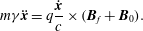
Having only the Lorentz force involved, the Lorentz factor is constant, and the equation of motion reads,
 $$\begin{eqnarray}m\unicode[STIX]{x1D6FE}\ddot{\boldsymbol{x}}=q\frac{\dot{\boldsymbol{x}}}{c}\times (\boldsymbol{B}_{f}+\boldsymbol{B}_{0}).\end{eqnarray}$$
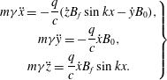
With the aforementioned choice of the fields, this equation splits into the three following scalar ones,
 $$\begin{eqnarray}\left.\begin{array}{@{}c@{}}\displaystyle m\unicode[STIX]{x1D6FE}\ddot{x}=-\frac{q}{c}({\dot{z}}B_{f}\sin kx-{\dot{y}}B_{0}),\\ \displaystyle m\unicode[STIX]{x1D6FE}\ddot{y} =-\frac{q}{c}{\dot{x}}B_{0},\\ \displaystyle m\unicode[STIX]{x1D6FE}\ddot{z}=\frac{q}{c}{\dot{x}}B_{f}\sin kx.\end{array}\right\}\end{eqnarray}$$
We now proceed to the following change of variables,
 $$\begin{eqnarray}\boldsymbol{x}\rightarrow \boldsymbol{X}/k,\quad B_{0}\rightarrow \unicode[STIX]{x1D6FC}B_{f},\quad t\rightarrow \unicode[STIX]{x1D70F}/\unicode[STIX]{x1D714}_{B},\quad \text{with}~\unicode[STIX]{x1D714}_{B}=\frac{qB_{f}}{\unicode[STIX]{x1D6FE}mc},\end{eqnarray}$$
and obtain the following equations,
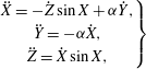 $$\begin{eqnarray}\left.\begin{array}{@{}c@{}}\ddot{X}=-{\dot{Z}}\sin X+\unicode[STIX]{x1D6FC}{\dot{Y}},\\ \ddot{Y} =-\unicode[STIX]{x1D6FC}{\dot{X}},\\ \ddot{Z}={\dot{X}}\sin X,\end{array}\right\}\end{eqnarray}$$
with initial conditions,
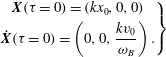 $$\begin{eqnarray}\left.\begin{array}{@{}c@{}}\boldsymbol{X}(\unicode[STIX]{x1D70F}=0)=(kx_{0},0,0)\\ \displaystyle \dot{\boldsymbol{X}}(\unicode[STIX]{x1D70F}=0)=\left(0,0,\frac{kv_{0}}{\unicode[STIX]{x1D714}_{B}}\right).\end{array}\right\}\end{eqnarray}$$
The case
 $\unicode[STIX]{x1D6FC}=0$
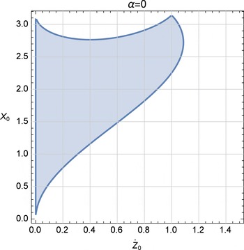
has already been treated (Bret Reference Bret2015). The domain of the phase space
 $({\dot{Z}}_{0},X_{0})$
where the particle bounces back against the region
 $z>0$
is pictured in figure 2. Whenever the initial conditions pertain to the shaded area, the particles come back to
 $z<0$
.
Case with no external
 $\boldsymbol{B}_{0}$
(
 $\unicode[STIX]{x1D6FC}=0$
) (Bret Reference Bret2015). Whenever the initial conditions pertain to the shaded area, the particles come back to
 $z<0$
. A particle launched from
 $X_{0}=\unicode[STIX]{x03C0}$
cannot bounce back since
 $\boldsymbol{B}_{f}(x=\unicode[STIX]{x03C0})=0$
.

In collisionless shock conditions, the interface at
 $z\sim 0$
is the location of important magnetic turbulence. As a consequence, particles starting from the shaded area do not systematically bounce back to
 $z<0$
, but tend to be trapped instead, in the region
 $z>0$
. In contrast, particles starting out of the shading area stream through the magnetic filaments.
Our goal from now on is to find out how figure 2 evolves when the external magnetic field
 $\boldsymbol{B}_{0}$
is switched on, that is, when
 $\unicode[STIX]{x1D6FC}\neq 0$
.
3 Analytical results
3.1 Symmetries
Although the full resolution of the problem will be numerical, a number of analytical considerations can pave the way to such resolution.
To start with, the system (2.4) is invariant by the substitutions
 $\unicode[STIX]{x1D6FC}\rightarrow -\unicode[STIX]{x1D6FC}$
and
 $X\rightarrow -X$
. It means an opposite
 $\boldsymbol{B}_{0}$
will simply have the particles spin in the opposite direction. But the
 $Z$
component, which determines whether the particle bounces back or not, is left unchanged. We can therefore restrict our study to
 $\unicode[STIX]{x1D6FC}>0$
, that is,
 $B_{0}>0$
.
Also, we can integrate the third equation of the system (2.4), and obtain regardless of
 $\unicode[STIX]{x1D6FC}$
,
 $$\begin{eqnarray}{\dot{Z}}(\unicode[STIX]{x1D70F})-{\dot{Z}}_{0}=\cos X_{0}-\cos X(\unicode[STIX]{x1D70F}).\end{eqnarray}$$
Since the velocity is constant, equal to
 $|\dot{\boldsymbol{X}}(\unicode[STIX]{x1D70F}=0)|={\dot{Z}}_{0}$
, the left-hand side remains negative along the trajectory. As a consequence,
 $\cos X(\unicode[STIX]{x1D70F})\geqslant \cos X_{0}$
,
 $\forall \unicode[STIX]{x1D70F}>0$
. Therefore, trajectories are bounded within intervals of width
 $2\unicode[STIX]{x03C0}$
and one can restrict the study to
 $X\in [-\unicode[STIX]{x03C0},\unicode[STIX]{x03C0}]$
(Bret Reference Bret2015).
Finally, the system (2.4) is also invariant when substituting
 $X\rightarrow -X$
and
 $Y\rightarrow -Y$
. This implies that we can restrict our attention to the interval
 $X\in [0,\unicode[STIX]{x03C0}]$
.
3.2 Equation for
 $X$
for
$Z>0$


The second equation of the system (2.4) can be integrated, giving
 $$\begin{eqnarray}{\dot{Y}}=-\unicode[STIX]{x1D6FC}(X-X_{0}).\end{eqnarray}$$
Inserting this result into the first equation of the system, and expressing
 ${\dot{Z}}$
in terms of
 $X$
with (3.1), we obtain the following equation for
 $X$
only,
 $$\begin{eqnarray}\ddot{X}+\sin X(\cos X_{0}+{\dot{Z}}_{0}-\cos X)+\unicode[STIX]{x1D6FC}^{2}(X-X_{0})=0.\end{eqnarray}$$
While it cannot be solved exactly, an approximated resolution is possible when
 $\sin X\sim 0$
.
3.3 Motion near
$X=0$

For
 $X_{0}\sim 0$
, we can write
 $\sin X\sim X$
and check later that
 $X(\unicode[STIX]{x1D70F})$
remains close to 0 for
 $\unicode[STIX]{x1D70F}>0$
. Equation (3.3) becomes after linearization,
 $$\begin{eqnarray}\ddot{X}+\unicode[STIX]{x1D714}^{2}X=\unicode[STIX]{x1D6FC}^{2}X_{0}\quad \text{with}~\unicode[STIX]{x1D714}^{2}=\unicode[STIX]{x1D6FC}^{2}+{\dot{Z}}_{0}>0.\end{eqnarray}$$
The solution reads,
 $$\begin{eqnarray}X(\unicode[STIX]{x1D70F})=\frac{\unicode[STIX]{x1D6FC}^{2}X_{0}}{\unicode[STIX]{x1D714}^{2}}+\frac{{\dot{Z}}_{0}X_{0}}{\unicode[STIX]{x1D714}^{2}}\cosh (\text{i}\unicode[STIX]{x1D714}\unicode[STIX]{x1D70F})\quad \text{with}~i^{2}=-1.\end{eqnarray}$$
With
 $\unicode[STIX]{x1D714}^{2}>0$
, trajectories oscillate between
 $X_{0}$
and
 $-X_{0}(1-2\unicode[STIX]{x1D6FC}^{2}/\unicode[STIX]{x1D714}^{2})$
, remaining thus confined around
 $X=0$
since
 $\unicode[STIX]{x1D6FC}^{2}<\unicode[STIX]{x1D714}^{2}$
.
We can then integrate the third equation of the system (2.4) to obtain an explicit expression for
 $Z(\unicode[STIX]{x1D70F})$
. The result is,
 $$\begin{eqnarray}Z(\unicode[STIX]{x1D70F})=\unicode[STIX]{x1D706}\unicode[STIX]{x1D70F}-\frac{{\dot{Z}}_{0}X_{0}^{2}}{4({\dot{Z}}_{0}+\unicode[STIX]{x1D6FC}^{2})^{5/2}}[4\unicode[STIX]{x1D6FC}^{2}+{\dot{Z}}_{0}\cosh (\text{i}\unicode[STIX]{x1D714}\unicode[STIX]{x1D70F})]\sinh (\text{i}\unicode[STIX]{x1D714}\unicode[STIX]{x1D70F}),\end{eqnarray}$$
with
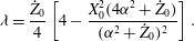 $$\begin{eqnarray}\unicode[STIX]{x1D706}=\frac{{\dot{Z}}_{0}}{4}\left[4-\frac{X_{0}^{2}(4\unicode[STIX]{x1D6FC}^{2}+{\dot{Z}}_{0})}{(\unicode[STIX]{x1D6FC}^{2}+{\dot{Z}}_{0})^{2}}\right].\end{eqnarray}$$
We may now find a condition for the particle to return to the region
 $Z<0$
, or to stream through the region
 $Z>0$
. The second term of (3.6) is oscillatory. But the first one, namely
 $\unicode[STIX]{x1D706}\unicode[STIX]{x1D70F}$
, tends to
 $\pm \infty$
depending on the sign of the parameter
 $\unicode[STIX]{x1D706}$
. We can indeed write
 $\lim _{\unicode[STIX]{x1D70F}+\infty }Z(\unicode[STIX]{x1D70F})=\text{sign}(\unicode[STIX]{x1D706})\infty$
. Therefore, our particle returns to
 $Z<0$
if
 $\unicode[STIX]{x1D706}<0$
, that is,
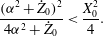 $$\begin{eqnarray}\frac{(\unicode[STIX]{x1D6FC}^{2}+{\dot{Z}}_{0})^{2}}{4\unicode[STIX]{x1D6FC}^{2}+{\dot{Z}}_{0}}<\frac{X_{0}^{2}}{4}.\end{eqnarray}$$
This expression bears interesting consequences. In the absence of an external magnetic field, that is,
 $\unicode[STIX]{x1D6FC}=0$
, the equation above gives
 ${\dot{Z}}_{0}<X_{0}^{2}/4$
(Bret Reference Bret2015). As can be seen in figure 2, the frontier between particles with
 $Z(\infty )=\pm \infty$
goes all the way down to
 $({\dot{Z}}_{0},X_{0})=(0,0)$
.
Now, setting
 $\unicode[STIX]{x1D6FC}\neq 0$
and
 ${\dot{Z}}_{0}=0$
in the equation above gives,
 $$\begin{eqnarray}-\unicode[STIX]{x1D6FC}<X_{0}<\unicode[STIX]{x1D6FC}.\end{eqnarray}$$
(Note that this conclusion reflects the
 $\pm X$
symmetry already mentioned.) As a consequence, particles starting from
 $X_{0}<\unicode[STIX]{x1D6FC}$
stream through the magnetized filaments, regardless of their initial velocity
 ${\dot{Z}}_{0}$
.
3.4 Motion near
$X=\unicode[STIX]{x03C0}$

For
 $X_{0}\sim \unicode[STIX]{x03C0}$
, we can write
 $\sin X\sim \unicode[STIX]{x03C0}-X$
and again, check afterward whether the trajectory remains confined near
 $X=\unicode[STIX]{x03C0}$
or not.
Setting
 $\tilde{X}=X-\unicode[STIX]{x03C0}$
and
 $\tilde{X}_{0}=X_{0}-\unicode[STIX]{x03C0}$
, and linearizing (3.3), we now obtain,
 $$\begin{eqnarray}\ddot{\tilde{X}}+\unicode[STIX]{x1D714}^{2}\tilde{X}=\unicode[STIX]{x1D6FC}^{2}\tilde{X}_{0}\quad \text{with}~\unicode[STIX]{x1D714}^{2}=\unicode[STIX]{x1D6FC}^{2}-{\dot{Z}}_{0},\end{eqnarray}$$
which solution reads,
 $$\begin{eqnarray}\tilde{X}(\unicode[STIX]{x1D70F})=\frac{\unicode[STIX]{x1D6FC}^{2}\tilde{X}_{0}}{\unicode[STIX]{x1D714}^{2}}-\frac{{\dot{Z}}_{0}\tilde{X}_{0}}{\unicode[STIX]{x1D714}^{2}}\cosh (\text{i}\unicode[STIX]{x1D714}\unicode[STIX]{x1D70F}).\end{eqnarray}$$
We need now to discuss the two cases corresponding to the sign of
 $\unicode[STIX]{x1D714}^{2}$
.
-
(i) If
$\unicode[STIX]{x1D714}^{2}<0$
, that is,
$\unicode[STIX]{x1D6FC}^{2}<{\dot{Z}}_{0}$
,
$\unicode[STIX]{x1D714}$
is purely imaginary and trajectories diverge on a time scale
$\unicode[STIX]{x1D70F}\sim |\unicode[STIX]{x1D714}|^{-1}$
, rendering expression (3.11) inaccurate. Note that
$B_{0}=0$
implies
$\unicode[STIX]{x1D6FC}=0$
, which means that in the absence of a guiding field, trajectories cannot remain confined (Bret Reference Bret2015). -
(ii) If
$\unicode[STIX]{x1D714}^{2}>0$
, that is,
$\unicode[STIX]{x1D6FC}^{2}>{\dot{Z}}_{0}$
, trajectories now oscillate between
$\tilde{X}_{0}$
and
$\tilde{X}_{0}^{+}=\tilde{X}_{0}(1+2\unicode[STIX]{x1D6FC}^{2}/\unicode[STIX]{x1D714}^{2})$
. Yet, in the present case where
$\unicode[STIX]{x1D6FC}^{2}>{\dot{Z}}_{0}$
we have
$\unicode[STIX]{x1D6FC}^{2}/\unicode[STIX]{x1D714}^{2}>1$
so that
$\tilde{X}_{0}^{+}$
may not remain close to zero. But if
$\tilde{X}_{0}^{+}\ll 1$
, the approximate solution (3.5) holds for any
$\unicode[STIX]{x1D70F}>0$
. We can linearize the third equation of the system (2.4) near
$X=\unicode[STIX]{x03C0}$
, obtaining for
$\tilde{X}(\unicode[STIX]{x1D70F})$
, (3.12)The solution can again be written as the sum of an oscillatory term, plus a term
$$\begin{eqnarray}\ddot{Z}=-\dot{\tilde{X}}\tilde{X}.\end{eqnarray}$$
$\unicode[STIX]{x1D706}\unicode[STIX]{x1D70F}$
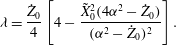
, with now (3.13)As was the case for
$$\begin{eqnarray}\unicode[STIX]{x1D706}=\frac{{\dot{Z}}_{0}}{4}\left[4-\frac{\tilde{X}_{0}^{2}(4\unicode[STIX]{x1D6FC}^{2}-{\dot{Z}}_{0})}{(\unicode[STIX]{x1D6FC}^{2}-{\dot{Z}}_{0})^{2}}\right].\end{eqnarray}$$
$X_{0}\sim 0$
, particles stream through the magnetized region if
$\unicode[STIX]{x1D706}>0$
. For
${\dot{Z}}_{0}\rightarrow 0^{+}$
, this implies (3.14)Particles meeting the condition above will stream through the
$$\begin{eqnarray}\tilde{X}_{0}^{2}<\unicode[STIX]{x1D6FC}^{2}\Rightarrow \unicode[STIX]{x03C0}-\unicode[STIX]{x1D6FC}<X_{0}<\unicode[STIX]{x03C0}+\unicode[STIX]{x1D6FC}.\end{eqnarray}$$
$Z>0$
region (note that the condition
$\unicode[STIX]{x1D6FC}^{2}>{\dot{Z}}_{0}$
, necessary to have
$\unicode[STIX]{x1D714}^{2}>0$
, is implicitly met for
${\dot{Z}}_{0}\rightarrow 0^{+}$
).










The forthcoming numerical study will confirm the conclusions of these two subsections, as evidenced in figure 4.
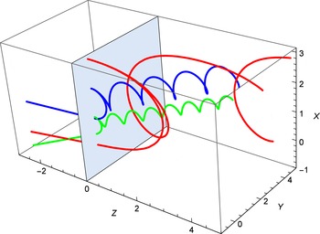
Numerical computation of a few trajectories. Red:
 $X_{0}=3$
,
 ${\dot{Z}}_{0}=1$
and
 $\unicode[STIX]{x1D6FC}=0$
or 0.2. Blue:
 $X_{0}=2$
,
 ${\dot{Z}}_{0}=0.5$
and
 $\unicode[STIX]{x1D6FC}=0$
or 0.5. Green:
 $X_{0}=1$
,
 ${\dot{Z}}_{0}=0.2$
and
 $\unicode[STIX]{x1D6FC}=0$
or 0.5. In each case, the trajectory with
 $\unicode[STIX]{x1D6FC}\neq 0$
goes to
 $Z=+\infty$
. The grey area features the plane
 $Z=0$
.

3.5 Canonical momenta
We here check that the constancy of two canonical momenta and of the Hamiltonian does not bring new information capable of pushing further our analytical exploration. The total magnetic field in the region
 $z>0$
reads
 $\boldsymbol{B}=(0,B_{f}\sin kx,B_{0})$
. It can be derived from the vector potential,
 $$\begin{eqnarray}\boldsymbol{A}=\left(0,B_{0}x,B_{f}\frac{\cos kx}{k}\right),\quad \text{with}~\unicode[STIX]{x1D735}\times \boldsymbol{A}=\boldsymbol{B}.\end{eqnarray}$$
The canonical momentum of a particle of mass
 $m$
and charge
 $q$
in the
 $z>$
region reads (Jackson Reference Jackson1998),
 $$\begin{eqnarray}\boldsymbol{P}=\boldsymbol{p}+\frac{q}{c}\boldsymbol{A},\end{eqnarray}$$
with
 $\boldsymbol{p}=\unicode[STIX]{x1D6FE}m\boldsymbol{v}$
. The canonical momentum
 $\boldsymbol{P}$
therefore only depends on the time derivative of the coordinates, and on the
 $x$
coordinate. It follows that the
 $y$
and
 $z$
coordinates of
 $\boldsymbol{P}$
are constants of the motion. Using the dimensionless variables (2.3a–c
), this reads
 $$\begin{eqnarray}\displaystyle \left.\begin{array}{@{}c@{}}\boldsymbol{P}_{y}=\boldsymbol{P}_{y}(t=0)\quad \Rightarrow \quad \unicode[STIX]{x1D6FC}X+{\dot{Y}}=\unicode[STIX]{x1D6FC}X_{0},\\ \boldsymbol{P}_{z}=\boldsymbol{P}_{z}(t=0)\quad \Rightarrow \quad {\dot{Z}}+\cos X={\dot{Z}}_{0}+\cos X_{0}.\end{array}\right\} & & \displaystyle\end{eqnarray}$$
The first equation of the system above is identical to (3.2), while the second is identical to (3.1). Furthermore, the constancy of the Hamiltonian
 $$\begin{eqnarray}{\mathcal{H}}=c\sqrt{m^{2}c^{2}+(c\boldsymbol{P}-q\boldsymbol{A})^{2}},\end{eqnarray}$$
reduces to
 $\boldsymbol{p}^{2}=\text{cst.}$
, which has already been accounted for through
 $\unicode[STIX]{x1D6FE}=\text{cst}$
.
4 Numerical study
Trajectories can be studied numerically using the NDSolve function of the Mathematica software. A series of 3D trajectories is pictured on figure 3. The two red trajectories both have
 $X_{0}=3$
and
 ${\dot{Z}}_{0}=1$
. But
 $\unicode[STIX]{x1D6FC}=0$
or 0.2 makes one bounce back, and the other go to
 $Z=+\infty$
. The two blue trajectories both have
 $X_{0}=2$
and
 ${\dot{Z}}_{0}=0.5$
. But
 $\unicode[STIX]{x1D6FC}=0$
or 0.5 makes one bounce back, and the other go to
 $Z=+\infty$
. Finally, the two green trajectories both have
 $X_{0}=1$
and
 ${\dot{Z}}_{0}=0.2$
. But
 $\unicode[STIX]{x1D6FC}=0$
or 0.5 makes one bounce back, and the other go to
 $Z=+\infty$
.
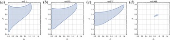
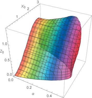
The evolution of figure 2 for
 $\unicode[STIX]{x1D6FC}$
varying up to
 ${\sim}0.5$
is pictured in figure 4. The expected shrinking of the shaded area at
 ${\dot{Z}}_{0}=0$
is observed, while a non-trivial reduction is also observed for
 ${\dot{Z}}_{0}>0$
. The overall picture makes perfect sense: as its relative intensity increases, the guiding magnetic field forces more and more particles to follow trajectories leading to
 $Z=+\infty$
.
Evolution of figure 2 for
 $\unicode[STIX]{x1D6FC}$
varying from 0.1 (a) up to
 ${\sim}0.5$
(d). Particles starting from the shaded area go back to
 $Z<0$
. This domain vanishes for
 $\unicode[STIX]{x1D6FC}>0.497$
, around
 $({\dot{Z}}_{0},X_{0})\sim (0.87,1.9)$
.

The 3D figure 5 allows for a unified perception of the cuts at
 $\unicode[STIX]{x1D6FC}=\text{cst.}$
represented in figure 4. One of the most remarkable features of this volume is that it is bounded. Whenever
 $\unicode[STIX]{x1D6FC}>1/2$
(rounding up 0.497 to
 $1/2$
), particles end up at
 $Z=+\infty$
, regardless of their initial conditions
 $({\dot{Z}}_{0},X_{0})$
. At such a level of external magnetization,
 $\boldsymbol{B}_{0}$
systematically overcomes the effect of the magnetic filaments. We shall now check the expected consequences on the formation of a parallel Weibel shock in pair plasmas.
3D representation of the shaded volume in the
 $({\dot{Z}}_{0},X_{0},\unicode[STIX]{x1D6FC})$
space, resulting from the assembling of the shaded areas at
 $\unicode[STIX]{x1D6FC}=\text{cst.}$
, like the ones pictured in figure 4. Parameters located inside the volume yield particle trajectories ultimately bouncing back to
 $Z<0$
. The colour code refers to the slices
 $\unicode[STIX]{x1D6FC}=\text{cst}$
.

5 Consequences for the formation of a parallel Weibel shock in pair plasmas
Assume two identical cold plasma shells with density
 $n_{0}$
, velocity
 $\pm \boldsymbol{v}_{0}$
and Lorentz factor
 $\unicode[STIX]{x1D6FE}_{0}$
heading towards each other. The system is embedded in an external magnetic field
 $\boldsymbol{B}_{0}\Vert \boldsymbol{v}_{0}$
. As they overlap, we assume the interaction is mediated by the Weibel instability, with growth rate (Stockem, Lerche & Schlickeiser Reference Stockem, Lerche and Schlickeiser2006),
 $$\begin{eqnarray}\frac{\unicode[STIX]{x1D6FF}}{\unicode[STIX]{x1D714}_{p}}=\sqrt{\unicode[STIX]{x1D6FF}_{0}^{2}-\unicode[STIX]{x1D6FA}_{B_{0}}^{2}},\quad \text{where}~\unicode[STIX]{x1D6FA}_{B_{0}}=\frac{1}{\unicode[STIX]{x1D714}_{p}}\frac{qB_{0}}{\unicode[STIX]{x1D6FE}mc},\end{eqnarray}$$
and
 $\unicode[STIX]{x1D6FF}_{0}=\unicode[STIX]{x1D6FD}\sqrt{4/\unicode[STIX]{x1D6FE}}$
is the growth rate, in
 $\unicode[STIX]{x1D714}_{p}$
units, when
 $B_{0}=0$
. The Weibel instability will generate magnetic filaments with a peak field
 $B_{f}$
at saturation fulfilling (Davidson et al.
Reference Davidson, Hammer, Haber and Wagner1972; Bret et al.
Reference Bret, Stockem, Fiúza, Ruyer, Gremillet, Narayan and Silva2013),
 $$\begin{eqnarray}\frac{qB_{f}}{\unicode[STIX]{x1D6FE}mc}=\unicode[STIX]{x1D6FF}\Leftrightarrow \unicode[STIX]{x1D6FF}_{0}^{2}=\unicode[STIX]{x1D6FA}_{B_{0}}^{2}+\unicode[STIX]{x1D6FA}_{B_{f}}^{2},\quad \text{where}~\unicode[STIX]{x1D6FA}_{B_{f}}=\frac{1}{\unicode[STIX]{x1D714}_{p}}\frac{qB_{f}}{\unicode[STIX]{x1D6FE}mc}.\end{eqnarray}$$
Writing now
 $B_{f}=B_{0}/\unicode[STIX]{x1D6FC}$
, we find that
 $\unicode[STIX]{x1D6FC}<1/2$
is equivalent to,
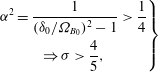 $$\begin{eqnarray}\displaystyle \left.\begin{array}{@{}c@{}}\displaystyle \unicode[STIX]{x1D6FC}^{2}=\frac{1}{(\unicode[STIX]{x1D6FF}_{0}/\unicode[STIX]{x1D6FA}_{B_{0}})^{2}-1}>\frac{1}{4}\\ \Rightarrow \unicode[STIX]{x1D70E}>\displaystyle \frac{4}{5},\end{array}\right\} & & \displaystyle\end{eqnarray}$$
where (we set
 $\unicode[STIX]{x1D6FD}=1$
),
 $$\begin{eqnarray}\unicode[STIX]{x1D70E}=\frac{B_{0}^{2}/4\unicode[STIX]{x03C0}}{\unicode[STIX]{x1D6FE}n_{0}mc^{2}},\end{eqnarray}$$
is the well-known magnetization parameter. For practical purposes, this parameter is usually much smaller than 1 in astrophysical environments, even in such strong magnetized environments as pulsar wind nebulae (Marcowith et al.
Reference Marcowith, Bret, Bykov, Dieckman, Drury, Lembège, Lemoine, Morlino, Murphy and Pelletier2016). Even
 $\unicode[STIX]{x1D70E}=10^{-1}$
results in
 $\unicode[STIX]{x1D6FC}=0.1$
, with effects hardly distinguishable from
 $\unicode[STIX]{x1D6FC}=0$
.
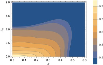
Since the two plasma shells are cold, the percentage of each shell which bounces back is simply obtained averaging our results over
 $X_{0}$
. The result of the calculation is displayed in figure 6, in terms of
 ${\dot{Z}}_{0}$
and
 $\unicode[STIX]{x1D6FC}$
. As long as
 $\unicode[STIX]{x1D6FC}\lesssim 0.4$
, the beam goes through the magnetic filaments region for
 ${\dot{Z}}_{0}>1$
, that is,
 $k^{-1}<v_{0}/\unicode[STIX]{x1D714}_{B}$
. In other words, the beam streams through the magnetic filaments if their size is smaller than the Larmor radius of the particles in the peak field
 $B_{f}$
. Beyond
 $\unicode[STIX]{x1D6FC}>1/2$
, the totality of the beam always goes to
 $z=+\infty$
.
Amount of each plasma shell bouncing back against the magnetic filaments region, as a function of
 ${\dot{Z}}_{0}$
and
 $\unicode[STIX]{x1D6FC}$
.

6 Conclusion
The formation of a Weibel shock involves the collision of two plasma shells. As they pass through each other, the overlapping region becomes Weibel unstable. At saturation, it forms magnetic filaments of transverse size
 $1/k$
and peak field
 $B_{f}$
. We have here determined under which conditions these filaments block the incoming flow, thus initiating the shock formation.
It has already been found that in the absence of an external magnetic field, most of the flow (if cold) keeps streaming through the filaments, or not, depending whether
 $1/k$
is smaller or larger than the Larmor radius of the particles in the field
 $B_{f}$
.
In the presence of a parallel magnetic field
 $\boldsymbol{B}_{0}$
, everything relies on the parameter
 $\unicode[STIX]{x1D6FC}=B_{0}/B_{f}$
. While
 $\unicode[STIX]{x1D6FC}\lesssim 0.4$
, the overall picture is similar to that with
 $\unicode[STIX]{x1D6FC}=0$
. But for
 $\unicode[STIX]{x1D6FC}>1/2$
a transition occurs. The guiding field
 $\boldsymbol{B}_{0}$
becomes dominant and particles keep streaming through the filaments regardless of their initial velocities. In realistic scenarios however, the parameter
 $\unicode[STIX]{x1D70E}$
, which governs the transition, forces
 $\unicode[STIX]{x1D6FC}\ll 1$
.
Further works could contemplate the case of a perpendicular field. Such a scenario involves more free parameters than the current one since the field would have to be specified by its two normal components, instead of one single parallel component as in the present case.
Acknowledgements
This work was supported by grant ENE2013-45661-C2-1-P from the Ministerio de Educación y Ciencia, Spain and grant PEII-2014-008-P from the Junta de Comunidades de Castilla-La Mancha.