1 Introduction
Over the last decade there has been a growing interest in fluid motion close to super-hydrophobic surfaces (SHSs) due to their potential application for drag reduction, initially in laminar flows (Watanabe, Udagawa & Udagawa Reference Watanabe, Udagawa and Udagawa1999; Rothstein Reference Rothstein2010) and recently in turbulent boundary layers as well (Min & Kim Reference Min and Kim2004; Bidkar et al.
Reference Bidkar, Leblanc, Kulkarni, Bahadur, Ceccio and Perlin2014; Park, Sun & Kim Reference Park, Sun and Kim2014). SHSs are typically constructed using a combination of micro- or/and nano-scale texture features and a hydrophobic surface chemistry (Liu, Tian & Jiang Reference Liu, Tian and Jiang2013). The hydrophobicity increases the local contact angle at the three phase contact line. Hence, it promotes the retention of micro air pockets between the asperities of the roughness, creating a partial air layer that separates the solid wall from the liquid (Rothstein Reference Rothstein2010). The net effect is similar to that achieved by injecting microbubbles in attempts to create lubricating air layers (Ceccio Reference Ceccio2010) but typically requires no energy input. However, when the textured surface is fully wetted and the dimensionless roughness expressed in wall units,
 $k^{+}=k/{\it\delta}_{{\it\upsilon}}$
, exceeds a critical value (Jimenez Reference Jimenez2004), the roughness increases the wall friction in turbulent boundary layers. Here,
 $k$
is the roughness height and
 ${\it\delta}_{{\it\upsilon}}$
is the viscous length scale (
 ${\it\upsilon}/u_{{\it\tau}}$
, the ratio between kinematic viscosity and friction velocity). The published values of
 $k^{+}$
for the onset of transition from smooth to rough regimes varies from
 $k^{+}=0.1$
(Ünal, Ünal & Atlar Reference Ünal, Ünal and Atlar2012),
 $k^{+}=1$
(Shockling, Allen & Smits Reference Shockling, Allen and Smits2006; Schultz & Flack Reference Schultz and Flack2007) to 15 (Ligrani & Moffat Reference Ligrani and Moffat1986), depending on the roughness type and uniformity. Therefore, SHSs consisting of rough boundaries may cause either drag increase, or reduction, depending on the roughness characteristics and Reynolds number Re of the flow. Based on experimental data, Bidkar et al. (Reference Bidkar, Leblanc, Kulkarni, Bahadur, Ceccio and Perlin2014) have recently reported that
 $k^{+}$
needs to be smaller than 0.5 for successful drag reduction, at least for the geometry used in their study. Direct numerical simulations (DNS) by Busse & Sandham (Reference Busse and Sandham2013) show that roughness with
 $k^{+}\sim 5$
extending above the air layer diminishes the drag reduction effects of SHSs. The objective of the present paper is to elucidate the competition and interplay between hydrophobicity and roughness effects through high-resolution near-wall velocity measurements within turbulent boundary layers developing over SHSs.
Numerical simulations have predicted appreciable turbulent drag reduction by SHSs, and have provided valuable physical insight into the processes involved. Most of these simulations have assumed ideal conditions, e.g. a flat air–water interface and no air loss. Simple surface textures have been simulated, such as posts (Martell, Rothstein & Perot Reference Martell, Rothstein and Perot2010), ridges (Jelly, Jung & Zaki Reference Jelly, Jung and Zaki2014) and sinusoidal grooves (Hasegawa, Frohnapfel & Kasagi Reference Hasegawa, Frohnapfel and Kasagi2011). The solid–liquid and air–liquid interfaces have been modelled either separately as no-slip and shear-free boundaries (Martell, Perot & Rothstein Reference Martell, Perot and Rothstein2009), or combined as an effective slip boundary (Min & Kim Reference Min and Kim2004; You & Moin Reference You and Moin2007), i.e. by assuming that:
 $$\begin{eqnarray}\displaystyle u|_{y=0}=u_{s}=\left.{\it\lambda}_{x}\frac{\partial u}{\partial y}\right|_{y=0},\quad v|_{y=0}=0,\quad w|_{y=0}=w_{s}=\left.{\it\lambda}_{z}\frac{\partial w}{\partial y}\right|_{y=0}, & & \displaystyle\end{eqnarray}$$
where
 $u$
,
 $v$
and
 $w$
are the streamwise
 $(x)$
, wall-normal
 $(y)$
and spanwise
 $(z)$
velocity components, respectively,
 $u_{s}$
and
 $w_{s}$
are the slip velocity components at the wall and
 ${\it\lambda}_{x}$
and
 ${\it\lambda}_{z}$
are components of the so-called slip lengths in directions indicated by the subscript. The existence of a non-zero streamwise slip length has several effects. (i) Significant drag reduction occurs when
 ${\it\lambda}_{x}$
is of the order of
 ${\it\delta}_{{\it\upsilon}}$
or larger, and this effect increases with
 ${\it\lambda}_{x}^{+}={\it\lambda}_{x}/{\it\delta}_{{\it\upsilon}}$
(Park, Park & Kim Reference Park, Park and Kim2013a
). For example, reduction of drag by more than 50 % has been predicted in the DNS studies by Martell et al. (Reference Martell, Rothstein and Perot2010). (ii) The mean velocity profile is shifted upward by
 $u_{s}^{+}$
(Jeffs, Maynes & Webb Reference Jeffs, Maynes and Webb2010) compared to that of the smooth wall. (iii) The peak magnitudes of all Reynolds stress components are significantly reduced but there is non-zero turbulence at the interface (Jelly et al.
Reference Jelly, Jung and Zaki2014). (iv) The streamwise vortical structures are suppressed (Park et al.
Reference Park, Park and Kim2013a
) and near-wall streaks are weakened (Min & Kim Reference Min and Kim2004; Busse & Sandham Reference Busse and Sandham2012). However, the existence of a finite spanwise slip length has the opposite effects, such as an increase in drag and Reynolds stresses, as well as a downward shift in the mean velocity profile (Fukagata et al.
Reference Fukagata, Kasagi and Koumoutsakos2006). When both
 ${\it\lambda}_{x}$
and
 ${\it\lambda}_{z}$
are non-zero, drag reduction is expected to be achieved when
 ${\it\lambda}_{x}\geqslant {\it\lambda}_{z}$
or when
 ${\it\lambda}_{x}^{+}>3.5$
for all values of
 ${\it\lambda}_{z}$
(Busse & Sandham Reference Busse and Sandham2012). High values of
 ${\it\lambda}_{x}$
and
 ${\it\lambda}_{z}$
can be obtained by increasing the air fraction of the SHSs, e.g. by increasing the spacing between micro-features for a fixed feature size (Jeffs et al.
Reference Jeffs, Maynes and Webb2010).
In reality, the air–water interface is neither flat nor steady, and the air layer can be continuously entrained by the liquid (Samaha, Vahedi Tafreshi & Gad-el-Hak Reference Samaha, Vahedi Tafreshi and Gad-el-Hak2011, Reference Samaha, Tafreshi and Gad-el-Hak2012; Seo, García-Mayoral & Mani Reference Seo, García-Mayoral and Mani2015), leading to a wetting transition and exposing the rough surface texture. Hence, it is essential to perform detailed velocity measurements near the SHS surface at realistic Reynolds numbers, which can be used for determining both the slip velocity and the local shear stresses. Furthermore, for large-scale applications, SHSs with random roughness are simpler to manufacture and apply than the idealized geometrical textures used in simulations, e.g. by spraying (Srinivasan et al. Reference Srinivasan, Chhatre, Mabry, Cohen and McKinley2011) or sand-blasting (Peguero & Breuer Reference Peguero and Breuer2009). One would expect that the behaviour of a boundary layer over a random roughness pattern is different from that of e.g. structured posts or ridges, considering that streamwise-aligned ridges can alone reduce drag (Choi et al. Reference Choi, Moin and Kim1993; García-Mayoral & Jiménez Reference García-Mayoral and Jiménez2011) regardless of surface chemistry. Yet, as will be shown in this study, the key findings of these earlier numerical and theoretical studies are broadly consistent with the experimental trends for random SHSs as well.
In parallel, numerous experimental studies have investigated the performance of SHSs in turbulent boundary layers (Henoch et al.
Reference Henoch, Krupenkin, Kolodner, Taylor, Hodes, Lynos, Peguero and Breuer2006), channel flows (Daniello, Waterhouse & Rothstein Reference Daniello, Waterhouse and Rothstein2009) and Taylor–Couette flows (Greidanus, Delfos & Westerweel Reference Greidanus, Delfos and Westerweel2011; Srinivasan et al.
Reference Srinivasan, Kleingartner, Gilbert, Cohen, Milne and McKinley2015). These tests have evaluated regularly patterned SHSs, such as ridges (Park, Sun & Kim Reference Park, Sun and Kim2013b
) and posts (Henoch et al.
Reference Henoch, Krupenkin, Kolodner, Taylor, Hodes, Lynos, Peguero and Breuer2006), as well as random roughness (Aljallis et al.
Reference Aljallis, Sarshar, Datla, Sikka, Jones and Choi2013). The roughness heights have ranged from nano-scale (Zhao, Du & Shi Reference Zhao, Du and Shi2007) to tens of microns (Bidkar et al.
Reference Bidkar, Leblanc, Kulkarni, Bahadur, Ceccio and Perlin2014). The skin frictions exerted on the textured surfaces have been quantified using floating surfaces connected to strain gages (Bidkar et al.
Reference Bidkar, Leblanc, Kulkarni, Bahadur, Ceccio and Perlin2014), as well as measuring the torque on the inner rotor in a Taylor–Couette facility (Greidanus et al.
Reference Greidanus, Delfos and Westerweel2011; Srinivasan et al.
Reference Srinivasan, Kleingartner, Gilbert, Cohen, Milne and McKinley2015) or the pressure drop in a channel flow (Jung & Bhushan Reference Jung and Bhushan2010). Studies involving application of particle image velocimetry (PIV) have typically resolved only the buffer and outer parts of the boundary layer
 $(y>5{\it\delta}_{{\it\upsilon}})$
(Daniello et al.
Reference Daniello, Waterhouse and Rothstein2009; Peguero & Breuer Reference Peguero and Breuer2009; Woolford et al.
Reference Woolford, Prince, Maynes and Webb2009; Tian et al.
Reference Tian, Zhang, Wang, Yao and Jiang2015; Vajdi Hokmabad & Ghaemi Reference Vajdi Hokmabad and Ghaemi2016). The velocity distributions have been used for examining the effects of SHSs on the flow structures and on the wall friction, the latter by fitting the mean velocity profiles in the log region (Tian et al.
Reference Tian, Zhang, Wang, Yao and Jiang2015), or by linearly extending the total stress profiles to the wall (Woolford et al.
Reference Woolford, Prince, Maynes and Webb2009). In a subset of these experiments, there has been no observable drag reduction, which the authors and later researchers have postulated to be a result of air layer depletion (Aljallis et al.
Reference Aljallis, Sarshar, Datla, Sikka, Jones and Choi2013), air layer vibrations (Zhao et al.
Reference Zhao, Du and Shi2007; Peguero & Breuer Reference Peguero and Breuer2009), dominance of wall roughness effects (Bidkar et al.
Reference Bidkar, Leblanc, Kulkarni, Bahadur, Ceccio and Perlin2014) as well as measurement uncertainties and errors (Greidanus et al.
Reference Greidanus, Delfos and Westerweel2011). However, other studies have successfully detected drag reduction with values that are consistent with the numerical results. In particular, they show that: (i) the drag reduction increases with increasing gas fraction (Park et al.
Reference Park, Sun and Kim2013b
, Reference Park, Sun and Kim2014) and Re, at least for set-ups involving channels at moderate Re (Daniello et al.
Reference Daniello, Waterhouse and Rothstein2009) and Taylor–Couette flows over a broad range of conditions (Srinivasan et al.
Reference Srinivasan, Kleingartner, Gilbert, Cohen, Milne and McKinley2015). For example, a maximum of 75 % reduction is reported by Park et al. (Reference Park, Sun and Kim2013b
, Reference Park, Sun and Kim2014) for SHSs consisting of streamwise-aligned micro-ridges with a 95 % gas fraction. (ii) By using spanwise-aligned ridges, Woolford et al. (Reference Woolford, Prince, Maynes and Webb2009) argue that spanwise slip increases drag. (ii) The mean velocity profile is shifted upward and the peak Reynolds shear stress decreases for
 ${\it\lambda}_{x}>0$
(Tian et al.
Reference Tian, Zhang, Wang, Yao and Jiang2015). Conversely, for
 ${\it\lambda}_{z}>0$
, the mean velocity is shifted downward and the Reynolds stress increases. (iv) SHSs suppress the sweep and ejection events and attenuate the spanwise vortical structures in the buffer layer (Vajdi Hokmabad & Ghaemi Reference Vajdi Hokmabad and Ghaemi2016).
Several notable theoretical studies have also attempted to predict and model the turbulent drag reduction induced by SHSs. Fukagata et al. (Reference Fukagata, Kasagi and Koumoutsakos2006) have introduced a functional relationship between drag reduction and slip length by matching the bulk mean velocity of the no-slip flow to that of the slip flow as:
 $$\begin{eqnarray}\displaystyle u_{{\it\tau}0}\left(\frac{1}{{\it\kappa}}\log \left(Re_{{\it\tau}}u_{{\it\tau}0}/u_{{\it\tau}}\right)+F({\it\lambda}_{z}^{+}=0)\right)=u_{{\it\tau}}\left({\it\lambda}_{x}^{+}+\frac{1}{{\it\kappa}}\log \left(Re_{{\it\tau}}\right)+F({\it\lambda}_{z}^{+})\right). & & \displaystyle\end{eqnarray}$$
Here
 $u_{{\it\tau}0}$
is the friction velocity of the no-slip flow,
 ${\it\kappa}=0.41$
is the von Kármán constant,
 $Re_{{\it\tau}}=u_{{\it\tau}}{\it\delta}/{\it\upsilon}$
is the friction Reynolds number (
 ${\it\delta}$
is the boundary layer thickness) and
 $F({\it\lambda}_{z}^{+})$
is a function of
 ${\it\lambda}_{z}^{+}$
. For the no-slip flow,
 $F({\it\lambda}_{z}^{+}=0)=3.2$
(Dean Reference Dean1978). For the slip flow,
 $F({\it\lambda}_{z}^{+})$
is obtained from empirical fitting to DNS results for flow with only spanwise slip. This model assumes that the effects of spanwise slip and streamwise slip are independent of each other, that
 ${\it\kappa}$
does not change and that drag reduction is caused solely by modification to the mean velocity profile. Substituting the
 ${\it\lambda}_{x}^{+}$
,
 ${\it\lambda}_{z}^{+}$
and
 $Re_{{\it\tau}}$
in (1.2), the calculated ratio of
 $u_{{\it\tau}}/u_{{\it\tau}0}$
agrees with their DNS results. Subsequently, Busse & Sandham (Reference Busse and Sandham2012) have proposed a modified
 $F({\it\lambda}_{z}^{+})$
, which requires few parameters for fitting the numerical simulation data. For SHSs in Taylor–Couette flows, Srinivasan et al. (Reference Srinivasan, Kleingartner, Gilbert, Cohen, Milne and McKinley2015) have proposed a modified Prandtl–von Kármán-type law to relate the skin friction coefficient to the slip length that is consistent within their range of Reynolds number
 $(10\,000<Re<80\,000)$
. For SHSs comprised of periodic post arrays, Seo & Mani (Reference Seo and Mani2016) have introduced a model for slip length as a function of the cubic root of the pattern wavelength, which agrees with their DNS results.
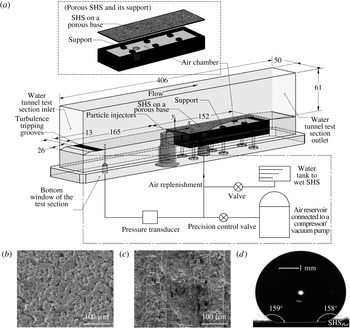
(a) The test section and the pressure control/measurement system; all dimensions are in mm; (b) a sample SEM image of
 $\text{SHS}_{Por}$
prior to spray coating it with F-POSS/PMMA; (c) a sample SEM image of
 $\text{SHS}_{Alx}$
with the streamwise etched grooves; and (d) a sample image of a
 ${\sim}270~{\rm\mu}\text{l}$
water droplet on
 $\text{SHS}_{Por}$
showing the equilibrium contact angles.

In summary, both numerical simulations and a number of prior experiments, have shown great promise for applying SHSs for turbulent drag reduction. However, due to the limited resolution of previous experimental studies, direct measurements of several key features are still unavailable. For example, the impact of SHSs on the profiles of mean velocity and turbulent parameters in the inner parts of boundary layers
 $(y<5{\it\delta}_{{\it\upsilon}})$
remains unclear. Importantly, the relative contributions between viscous and Reynolds stress components have not been resolved considering that slip can occur over a substantial fraction of the wall. Furthermore, the slip velocity and the slip length have not been measured directly in turbulent flows. Thus, the functional relations between
 ${\it\lambda}_{x}^{+}$
,
 ${\it\lambda}_{z}^{+}$
and drag reduction proposed in the theoretical (Fukagata et al.
Reference Fukagata, Kasagi and Koumoutsakos2006; Busse & Sandham Reference Busse and Sandham2012) and numerical (Park et al.
Reference Park, Park and Kim2013a
) studies have not been verified. Thus, the present paper focuses on measuring the flow structure and Reynolds stresses very close to the wall
 $(y<5{\it\delta}_{{\it\upsilon}})$
for several different SHSs, including direct measurements of the local wall friction and slip velocity. By extending the range of boundary layer Reynolds numbers, we also show that a single surface can transition from reducing drag to increasing drag, as
 $k^{+}$
increases above a certain threshold level, corresponding to when the roughness effects dominate. To maintain and replenish the air layer, porous substrates for the SHSs are also used with controlled pressure difference across the porous wall. The experimental set-up is described in § 2, followed by presentation of results in § 3 and a discussion and conclusions in § 4.
2 Experimental set-up and techniques
The experiments have been performed in a small, high-speed water tunnel described in Gopalan & Katz (Reference Gopalan and Katz2000) and Liu & Katz (Reference Liu and Katz2006). The flow is driven by two 15 HP (maximum) centrifugal pumps located 5 m below the test section, and passes through a settling tank, an electromagnetic flow meter, a settling chamber containing honeycombs and screen as well as a 9 : 1 contraction before entering the test section. Components relevant to the present study, as they are installed in the 406 mm long, 61 mm high and 50 mm wide transparent test section, are sketched in figure 1(a). The mean tunnel speeds (flow rate divided by the tunnel cross-section),
 $U_{m}$
, are between 2 and 20[[()[]!--\jatstusp--[]()]] m[[()[]!--\jatstusp--[]()]] s-1. At the entrance to the test section, the bottom window contains a series of machined spanwise tripping grooves, which are located 165 mm (9–22 boundary layer heights) upstream of the SHSs. The purpose of these grooves is to force early boundary layer transition to turbulence, as shown in prior studies (Liu & Katz Reference Liu and Katz2013). The 152 mm long and 50 mm wide SHS is flush mounted on the same wall. The coordinate system is also shown, with
 $x$
,
 $y$
and
 $z$
denoting the streamwise, wall-normal and spanwise directions, respectively, and with
 $x=0$
coinciding with the leading edge of the SHS, all consistent with the coordinates used in the Introduction.
The SHSs have been created on both porous stainless steel bases and non-porous aluminium bases, denoted as
 $\text{SHS}_{Por}$
and
 $\text{SHS}_{Al}$
, respectively. The
 $\text{SHS}_{Por}$
is manufactured by spray coating a mixture of a poly methyl methacrylate (PMMA) binder and fluorinated polyhedral oligomeric silsesquioxane (F-POSS) using procedures described in Srinivasan et al. (Reference Srinivasan, Chhatre, Mabry, Cohen and McKinley2011). The reason for using a porous substrate as a base is to provide a means for continuously replenishing the micro air pockets that are gouged away and entrained by the flow. A sample scanning electron micrograph (SEM) of the porous bases prior to spraying is shown in figure 1(b). They have a permeability of
 $0.27{-}0.98~{\rm\mu}\text{m}^{2}$
(
 $1/700$
–
 $1/200$
acfm
 $\cdot$
cp
 $\cdot$
inch/psid/ft
 $^{2}$
) and porosity of 17–26 %, as specified by the manufacturers. The size of particles forming the bases as seen in the SEM images (since the manufacturer does not provide them) varies from 20 to
 $40~{\rm\mu}\text{m}$
. The porous bases are tightly glued to six
 $6.4\times 6.4~\text{mm}^{2}$
support legs and 5.2 mm wide edges, leaving
 ${\sim}70\,\%$
of their underside exposed to an air chamber. This chamber is connected through valves to a compressor and a vacuum pump, allowing us to set it at desired pressures
 $P_{1}$
. The pressure in the test section,
 $P_{2}$
, is also controlled by connecting the same compressor and vacuum pump to an air–water interface located in a chamber well above the test section (Gopalan & Katz Reference Gopalan and Katz2000). The pressure difference across the porous wall,
 ${\rm\Delta}P=P_{2}-P_{1}$
can be varied and is monitored by a pressure transducer.
The
 $\text{SHS}_{Al}$
is manufactured by polishing an aluminium base manually, and then etching it in hydrochloric acid, boiling it in water and coating it with (heptadecafluoro-1,1,2,2-tetrahydrodecyl) trichlorosilane using vapour deposition. Further details are provided in Yang et al. (Reference Yang, Zhang, Xu, Men, Zhu and Zhou2011). Two different subtypes of
 $\text{SHS}_{Al}$
are involved in this study. For the first, surface polishing is performed in random directions and the resulting surface is denoted
 $\text{SHS}_{Alr}$
. For the second, denoted
 $\text{SHS}_{Alx}$
, the chemical treatment and silanization procedure are kept the same, but the polishing is intentionally aligned in the
 $x$
direction forming preferentially streamwise grooves that have spatially non-uniform spacing and depth. The average spacing, as determined by a laser interferometry, is
 $110~{\rm\mu}\text{m}$
. A sample SEM image of
 $\text{SHS}_{Alx}$
is shown in figure 1(c). For these samples,
 ${\rm\Delta}P$
is used to denote the pressure difference between
 $P_{2}$
and atmosphere pressure when we examine the effects of compressing the air layer on the skin friction. To characterize the SHSs before the water tunnel tests, the static contact angles and sliding angles of water droplets on the surfaces are measured. The contact angles are calculated by recording images of static
 ${\sim}4~\text{mm}$
(
 ${\sim}270~{\rm\mu}\text{l}$
) water droplets situated on the SHSs, e.g. figure 1(d). The sliding angles are determined by slowly tilting the SHSs until the droplets start moving and rolling off of the surfaces.
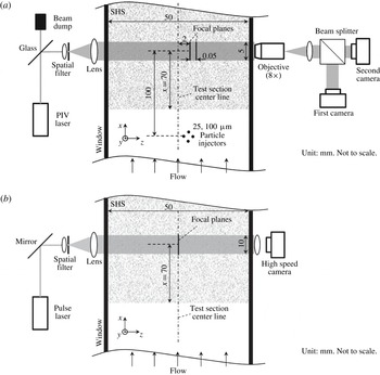
Illustrations of (a) the dual view in-line digital holographic microscopy set-up for high-resolution velocity measurements; and (b) the holographic set-up for imaging the air layer or ‘plastron’ present on the SHSs.

The optical set-up for performing high-resolution velocity measurements is illustrated in figure 2(a). To fully resolve the flow in the inner part of the boundary layer, we have opted to use in-line digital holographic microscopy (DHM). Since we cannot record holograms through the SHSs, we have developed a new approach to record DHM data in ‘deep’ samples, as described in detail by Ling & Katz (Reference Ling and Katz2014) In-line holographic reconstruction creates twin three-dimensional (3-D) images located symmetrically on both sides of the hologram plane. Thus, placing the hologram plane in the middle of the sample volume (i.e. to sustain submicron resolution), particles located on one side of the hologram will be reconstructed on both sides, ‘mixing’ them. To overcome this problem, we record a pair of holograms whose planes are separated by a short distance from each other. The real particle fields of both images coincide, whereas the virtual/twin ones are separated by twice the distance between planes. The software and procedures are discussed in detail and demonstrated in Ling & Katz (Reference Ling and Katz2014). The light source is an Nd–YAG laser (532 nm). Since very little energy is required for in-line DHM, only light reflected from an uncoated flat glass surface is used. The beam is spatially filtered, expanded and collimated to 5 mm diameter before illuminating the sample volume. The flow is seeded locally with 2
 ${\rm\mu}\text{m}$
silver-coated glass particles. To minimize the effect of injection on the flow, the particles are injected at a low speed of less than
 $0.08U_{m}$
from 25 evenly distributed 100
 ${\rm\mu}\text{m}$
holes located
 ${\geqslant}$
100 mm (1000 injector diameters) upstream of the sample volume. The light scattered by these particles interferes with the remainder of the collimated beam to form the in-line hologram. An
 $8\times$
infinity-corrected, long working distance microscope objective magnifies the images, while focusing on the selected hologram planes. A cube beam splitter directs the images to two interline transfer digital cameras (Imperx ICL-B6640,
 $4400\times 6600$
pixels,
 $5.5~{\rm\mu}\text{m}~\text{pixel}^{-1}$
) generating a pair of holograms. Their focal planes are located approximately 2 mm away from the centre of the test section, separated by 50
 ${\rm\mu}\text{m}$
and at
 $x=70~\text{mm}$
, as shown in figure 2(a). They have calibrated spatial resolutions of 0.677 and
 $0.685~{\rm\mu}\text{m}~\text{pixel}^{-1}$
. The total sample area cross-section is
 $4.4\times 2.4~\text{mm}^{2}$
(
 $x\times y$
) and the total depth of the interrogated volume extends to 3.2 mm in the
 $z$
direction for most cases. However, as discussed below, this domain is divided into multiple sample volumes, which are interrogated separately.
High-speed digital holography has been used to monitor the air layer interface and to measure the entrainment rate of air from the
 $\text{SHS}_{Por}$
, as sketched in figure 2(b). Here, the light source is a Q-switched Nd:YLF laser (523 nm) whose output is expanded and collimated to a 10 mm diameter beam. The holograms are recorded by a high-speed camera (PCO.Dimax HD) at
 $20\,000~\text{frames}~\text{s}^{-1}$
and at a resolution of
 $11~{\rm\mu}\text{m}~\text{pixel}^{-1}$
. The sample volume is centred at
 $x=70$
mm, and has a streamwise length of 9.5 mm, a wall-normal height of 2.5 mm and a depth of 50 mm, the latter covering the entire depth of the water tunnel. Three sample high-speed movies of original holograms of the air layer on the
 $\text{SHS}_{Por}$
for
 $U_{m}$
varying between 2 and
 $6~\text{m}~\text{s}^{-1}$
, and
 ${\rm\Delta}P$
varying between
 $-4.0$
and 12 kPa, are in the supplementary data available at http://dx.doi.org/10.1017/jfm.2016.450. They provide direct confirmation that an air layer or plastron (Shirtcliffe, McHale & Newton Reference Shirtcliffe, McHale and Newton2011) is indeed attached to the
 $\text{SHS}_{Por}$
, and this interface fluctuates at increasing surface speeds with increasing
 $U_{m}$
. To measure the size distribution of bubbles and their cumulative volume, the holograms are reconstructed every 100
 ${\rm\mu}\text{m}$
. The 3-D intensity field is subsequently collapsed into a single plane, where each pixel has the minimum intensity (darkest) over the entire depth. The collapsed image is thresholded and segmented to identify each bubble and obtain its size. The flux of bubbles is calculated by dividing the cumulative volume of all the bubbles in the sample volume, averaged over eight realizations, by the time that is required for them to pass through the sample volume. This time is estimated by dividing the length of the sample area by the height-dependent mean streamwise velocity of the fluid. This flux is used for estimating the rate of bubbles entrained from the upstream 70 mm of the porous surface (3500 mm2). This estimate is smaller than the actual entrainment rate since some of the bubbles might be lifted to elevations located above the sample volume. However, by tracking the vertical bubble flux at different elevations and determining that it is negligible at the top of the sample volume, and by insuring that the buoyancy alone is insufficient to lift the bubbles away from the field of view, the overwhelming majority (
 ${>}$
99 %) of the bubbles entrained from the wall remain inside the sample volume. It should also be noted that without the air layer, there are no free stream bubbles with resolvable sizes near the bottom wall. The entrainment rate of the bubbles is then divided by the surface area and
 $U_{m}$
to obtain the dimensionless, spatially and time-averaged air velocity
 $U_{air}^{\ast }$
.
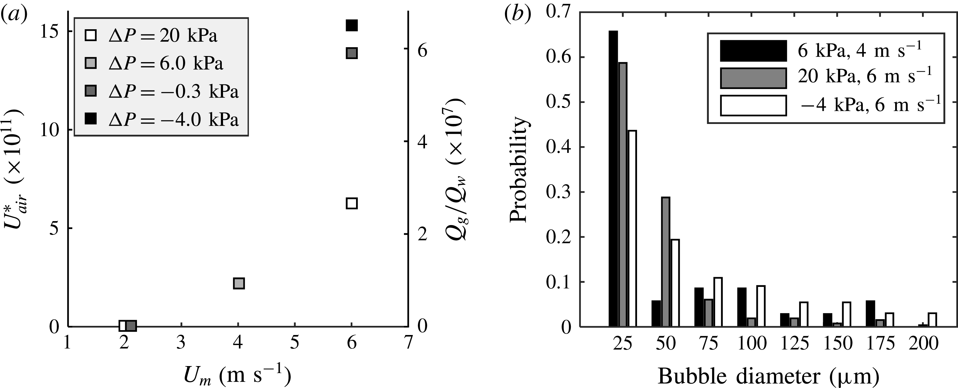
As expected,
 $U_{air}^{\ast }$
increases with increasing
 $U_{m}$
and decreasing
 ${\rm\Delta}P$
, as shown in figure 3(a). For
 $U_{m}=2.0~\text{m}~\text{s}^{-1}$
(
 $Re_{{\it\tau}}=1408$
, as shown later),
 $U_{air}^{\ast }$
is essentially zero, i.e. the wall shear stresses fall below the threshold required for entraining the air. It increases to
 $1.5\times 10^{-10}$
at
 $U_{m}=6.0~\text{m}~\text{s}^{-1}$
and
 ${\rm\Delta}P=-4.0$
kPa. Furthermore, using a separate axis, figure 3(a) also shows the ratio of the gas to liquid flow rates in the boundary layer,
 $Q_{g}/Q_{w}$
. As shown, the maximum value of this ratio is approximately
 $7\times 10^{-7}$
. According to Ceccio (Reference Ceccio2010) and Ferrante & Elghobashi (Reference Ferrante and Elghobashi2004), to achieve drag reduction by injecting air bubbles, this ratio has to be of the order of
 $10^{-3}$
or higher. Therefore, the present bubble concentration is at least three orders of magnitude lower than that required for affecting the drag force. Sample ensemble-averaged size distributions of entrained bubbles are shown in figure 3(b). The results for
 $U_{m}=2.0~\text{m}~\text{s}^{-1}$
is not included since it is zero, but the rest demonstrate that the number of ‘large’ bubbles (
 ${>}50~{\rm\mu}\text{m}$
) increases with entrainment rate. However, the high-speed movies confirm that both the air layer and the steady entrainment of bubbles are maintained on the
 $\text{SHS}_{Por}$
for more than four hours for the entire current range of
 $U_{m}$
and
 ${\rm\Delta}P$
, presumably because of the continuous replenishment of the plastron by air under the porous surface. The persistence of the entrainment for
 $0<{\rm\Delta}P<20$
kPa indicates that the capillary forces are sufficient for overcoming the air layer suppression by the higher pressure in the test section. To remove the air layer in some experiments, the entire space under the porous base has to be filled with water. We have not tried pressures exceeding
 ${\rm\Delta}P=20$
kPa, fearing that it might damage the substrate.
(a) Normalized entrainment rate of air (
 $U_{air}^{\ast }$
and
 $Q_{g}/Q_{w}$
) from the
 $\text{SHS}_{Por}$
upstream of the sample area for several pressure differences across the porous wall; (b) the measured size distribution of the entrained bubbles.

The optical set-up of figure 2(a) with the same magnification and sample area is used to evaluate and quantify the topographies of each
 $\text{SHS}_{Por}$
and
 $\text{SHS}_{Alr}$
. The local roughness height
 $h(x)$
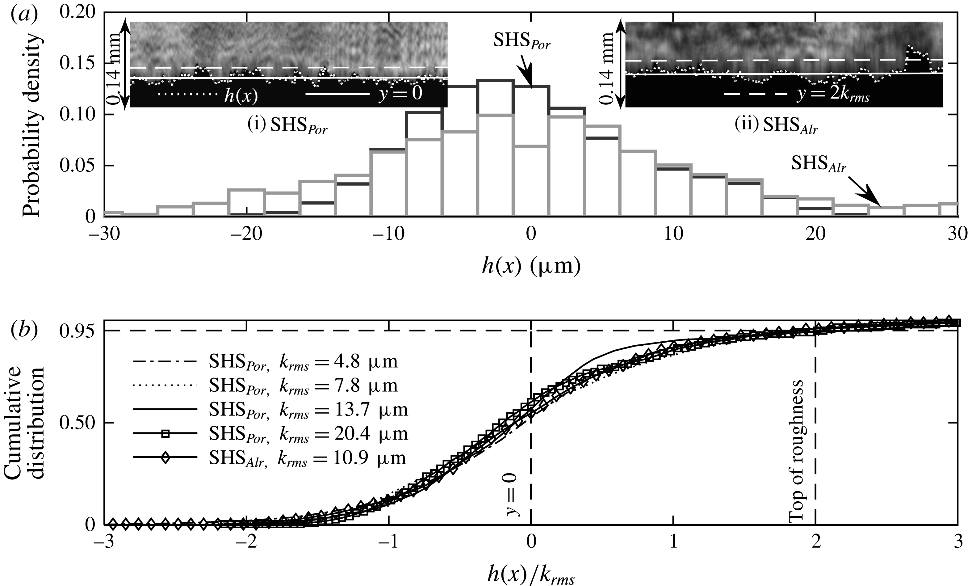
is estimated directly from the projection of the roughness peaks on the holograms. The holograms are recorded while the facility is running, filled with water, at the same velocities as those used during the actual measurements. By selecting a threshold of intensity to include roughness elements which are nearly in focus, the projected ridgeline is tracked, as illustrated in the inserts in figure 4(a). For the sample holograms of
 $\text{SHS}_{Por}$
and
 $\text{SHS}_{Alr}$
presented in the inserts,
 $U_{m}=2~\text{m}~\text{s}^{-1}$
. Figure 4(a) also shows the two corresponding histograms of
 $h(x)$
. This procedure is aimed at characterizing the roughness height under conditions that best represent the surface shape during the velocity and turbulence measurements. Thus, the
 $h(x)$
accounts for the presence of the air layer. Since the histograms of
 $h(x)$
appear to be nearly Gaussian, we opt to characterize the roughness height using the root mean square value of
 $h(x)$
, and denote it as
 $k_{rms}=(\int h^{2}\,\text{d}x)^{0.5}/L$
, where
 $L$
is the sample length. For the present measurements, the magnitude of
 $k_{rms}$
of the
 $\text{SHS}_{Por}$
ranges from 4.8 to 20.4
 ${\rm\mu}\text{m}$
and that of the
 $\text{SHS}_{Alr}$
is 10.9
 ${\rm\mu}\text{m}$
, with an uncertainty of approximately 1
 ${\rm\mu}\text{m}$
. Figure 4(b) shows the cumulative distributions of
 $h(x)$
for five values of
 $k_{rms}$
. The holograms are not suitable for characterizing the roughness height of
 $\text{SHS}_{Alx}$
since the roughness elements are not projected outward. Therefore, for
 $\text{SHS}_{Alx}$
, we utilize a laser interferometer with a resolution of approximately 1
 ${\rm\mu}\text{m}$
in both
 $x$
and
 $z$
directions to measure the height distribution. The values of
 $k_{rms}$
of the
 $\text{SHS}_{Alx}$
in the flow measurement area (
 $x=70$
mm) is 8.9
 ${\rm\mu}\text{m}$
. To obtain an estimate of the uncertainty in
 $k_{rms}$
, the laser interferometer has also been applied to obtain independent measurements of roughness for one of the
 $\text{SHS}_{Por}$
and the
 $\text{SHS}_{Alr}$
. The results give
 $k_{rms}$
values that are lower by 10–20 % than those obtained from the holograms. Hence, this difference is used as a rough estimate of our uncertainty in roughness measurements.
(a) Sample probability density functions of the roughness height
 $h(x)$
for one of the
 $\text{SHS}_{Por}$
(
 $k_{rms}=7.8~{\rm\mu}\text{m}$
, case no. 8) and the
 $\text{SHS}_{Alr}$
(case no. 4). The insets show corresponding sample holograms. Dotted lines:
 $h(x)$
, solid lines: mean roughness height (
 $y=0$
) and dashed lines:
 $y=2k_{rms}$
. (b) Cumulative distribution of
 $h(x)$
for several
 $k_{rms}$
.

The present surface geometries and composition prevent us from providing a reliable scale for the roughness spacing, especially if one wants to compare surfaces. Spraying inherently involves a multiscale surface pattern. Thus, evaluating the surface only based on the observed peaks is questionable, since much smaller crevices might affect the trapping of air as well. We estimate the mean spacing between roughness elements by counting the total number of maxima that exceed two local standard deviations of the local mean height. Assuming they are distributed randomly within the hologram depth of focus
 ${\sim}200~{\rm\mu}\text{m}$
(without reconstruction), the characteristic roughness wavelength
 ${\it\alpha}$
for the
 $\text{SHS}_{Por}$
and
 $\text{SHS}_{Alr}$
falls in
 $90~{\rm\mu}\text{m}<{\it\alpha}<100~{\rm\mu}\text{m}$
. This value does not differ significantly among different samples, even though the magnitude of
 $k_{rms}$
does change. The magnitude and distribution of
 ${\it\alpha}$
should also be accounted for while characterizing the efficacy of the SHS or roughness effects. However, due to the higher confidence in its magnitude, we opt to characterize the surfaces based on
 $k_{rms}$
. The randomly distributed roughness also prevents us from quantifying the gas fraction for the different surfaces and flow conditions.
The location of
 $y=0$
is selected as the mean roughness height, consistent with previous rough walls studies (Brzek et al.
Reference Brzek, Cal, Johansson and Castillo2008; Chan et al.
Reference Chan, Macdonald, Chung, Hutchins and Ooi2015). It is indicated by solid lines in the insets of figure 4(a). To minimize the potential effects of form drag, the wall friction and slip velocity are calculated at the top of the roughness, which is selected as the elevation where the cumulative distribution of
 $h(x)$
reaches 95 %, namely
 $y=2k_{rms}$
. The location of this elevation is indicated by the dashed lines in the insets of figure 4(a) and in figure 4(b). While one could also define the top of the roughness as the point where the cumulative distribution of
 $h(x)$
reaches e.g. 90 % or 99 %, the impact of this choice on the uncertainties in slip velocity and wall friction is discussed and accounted for later. The present choice for
 $y=0$
facilitates displaying the velocity and stress profiles at the top of the roughness, namely at
 $y=2k_{rms}$
. Altering this reference height within the roughness domain has not led to collapse of data, but has caused loss of data near the point where the wall stress is evaluated. It has negligible effect on the mean profile in the log region and does not change the overall trends.
To calculate the velocity field from the high-resolution holograms obtained from the set-up described in figure 2(a), the following data analysis procedures are employed. First, to reconstruct only the real particle images, we use a phase based reconstruction (Denis et al.
Reference Denis, Fournier, Fournel and Ducottet2005; Ling & Katz Reference Ling and Katz2014), which involves a spatial convolution of both the intensity and phase (complex amplitude) distribution in (one of) the hologram plane with a Rayleigh–Sommerfeld kernel (Katz & Sheng Reference Katz and Sheng2010). The phase distribution is estimated iteratively by propagating the wave field back and forth between the two hologram planes using diffraction theory (Denis et al.
Reference Denis, Fournier, Fournel and Ducottet2005). This phase based reconstruction is performed every 13
 ${\rm\mu}\text{m}$
in depth to generate a series of closely spaced planes containing real images only. Then, following Sheng, Malkiel & Katz (Reference Sheng, Malkiel and Katz2008) and Talapatra & Katz (Reference Talapatra and Katz2013), the 3-D fields are segmented to generate the spatial distribution of particles, followed by particle tracking to match particle traces in the hologram pairs. Between 6000 and 10 000 particles pairs are typically matched in each of the
 $4.4\times 2.4\times 3.2~\text{mm}^{3}\;(x\times y\times z)$
sample volumes. Matching involves seven criteria, including similarity of particle size, shape and intensity, as well as smoothness of the velocity field and agreement with guess 2-D vectors generated using standard PIV cross-correlations of images created by compressing the entire volume into a plane. Symbols
 $u$
,
 $v$
and
 $w$
are used to denote the instantaneous velocity components in the
 $x$
,
 $y$
and
 $z$
directions respectively. The magnitudes of
 $u$
and
 $v$
are calculated from the in-plane centroids of the particles and
 $w$
is calculated based on locations of minimum intensity within the elongated traces of particle in the spanwise direction. The accuracy of
 $w$
is lower compared to
 $u$
and
 $v$
but could be improved by locating the centre of the particles using edge detection (Talapatra & Katz Reference Talapatra and Katz2013) or correlations among the elongated traces (Ling & Katz Reference Ling and Katz2014). However, as the focus of this paper is on the distributions of
 $u$
and
 $v$
, additional effort is not invested in improving the accuracy of
 $w$
. The sample volume is divided into multiple small windows with a size of
 $10{\it\delta}_{{\it\upsilon}}\times 1{\it\delta}_{{\it\upsilon}}\times 10{\it\delta}_{{\it\upsilon}}\;(x\times y\times z)$
for
 $U_{m}=2~\text{m}~\text{s}^{-1}$
and
 $20{\it\delta}_{{\it\upsilon}}\times 1{\it\delta}_{{\it\upsilon}}\times 20{\it\delta}_{{\it\upsilon}}\;(x\times y\times z)$
for
 $U_{m}=6~\text{m}~\text{s}^{-1}$
. Only the windows containing particles are included in the statistical analysis for each volume. More than 1000 instantaneous velocity fields are processed and ensemble-averaged locally for each window to obtain the mean (dented as
 $U$
and
 $V$
) and the corresponding Reynolds normal and shear stress components,
 $\langle u^{\prime }u^{\prime }\rangle$
,
 $\langle v^{\prime }v^{\prime }\rangle$
and
 $\langle u^{\prime }v^{\prime }\rangle$
. Results are then spatially averaged in the
 $x$
and
 $z$
directions to obtain data that are not dependent on the local roughness patterns. Spatially averaged values are denoted with an over bar, e.g.
 $\overline{U}$
,
 $\overline{\langle u^{\prime }v^{\prime }\rangle }$
, and etc.
For
 $\text{SHS}_{Por}$
, the measurement domain starts from
 $y=0$
, and the first data point included in this paper is located at
 $y={\it\delta}_{{\it\upsilon}}$
. This point is located below the tip of the roughness elements. For
 $\text{SHS}_{Alr}$
, the measurement domain starts from
 $y=k_{rms}$
and the first data point is located at
 $y=k_{rms}+{\it\delta}_{{\it\upsilon}}\approx 2k_{rms}$
. For
 $\text{SHS}_{Alx}$
, we cannot examine the space between the roughness elements. Therefore, the location of
 $y=0$
can only be estimated based on observed particles attached to the surface. Hence, the first data point is located at
 $y\approx 2k_{rms}+1{\it\delta}_{{\it\upsilon}}$
. The values of the mean spatially averaged viscous stress,
 ${\it\tau}^{{\it\mu}}$
, are calculated using
 ${\it\tau}^{{\it\mu}}={\it\mu}\partial \overline{U}/\partial y$
, where
 ${\it\mu}=1\times 10^{-3}~\text{kg}~\text{m}^{-1}~\text{s}^{-1}$
. Since the mean velocity profiles for the smooth walls, the
 $\text{SHS}_{Por}$
with
 $k_{rms}\leqslant {\it\delta}_{{\it\upsilon}}$
and the
 $\text{SHS}_{Alr}$
are nearly linear at
 $y\leqslant 5{\it\delta}_{{\it\upsilon}}$
, the values for
 $y<3{\it\delta}_{{\it\upsilon}}$
are calculated by linearly fitting the mean velocity profiles based on the
 $y\leqslant 5{\it\delta}_{{\it\upsilon}}$
data. However, for the SHSs with
 $k_{rms}>{\it\delta}_{{\it\upsilon}}$
, the mean profiles are not linear at
 $y\leqslant 5{\it\delta}_{{\it\upsilon}}$
. Thus,
 ${\it\tau}^{{\it\mu}}$
at
 $y={\it\delta}_{{\it\upsilon}}$
(first point) is not available, second-order finite differencing is used for
 $y=2{\it\delta}_{{\it\upsilon}}$
, and 5 points are used for higher elevations. The total stress
 ${\it\tau}_{t}={\it\tau}^{{\it\mu}}+{\it\tau}^{R}$
is determined by adding
 ${\it\tau}^{{\it\mu}}$
and the spatially averaged Reynolds shear stress,
 ${\it\tau}^{R}=-{\it\rho}\overline{\langle u^{\prime }v^{\prime }\rangle }$
, where
 ${\it\rho}=1\times 10^{3}~\text{kg}~\text{m}^{-3}$
. The wall viscous stress
 ${\it\tau}_{w}^{{\it\mu}}$
, wall Reynolds shear stress
 ${\it\tau}_{w}^{R}$
and total wall friction
 ${\it\tau}_{w}$
are determined from the corresponding stresses at
 $y=$
0 for smooth walls,
 $y=2k_{rms}$
for
 $\text{SHS}_{Por}$
and
 $\text{SHS}_{Alr}$
and at
 $y=2k_{rms}+1{\it\delta}_{{\it\upsilon}}$
for
 $\text{SHS}_{Alx}$
. To estimate the slip velocity, we calculate the mean and spatially averaged velocity at
 $y=2k_{rms}$
, and denote it by
 $\overline{U}_{s}$
.
The uncertainty in velocity measurements is based on prior studies where many of the present tools for applying digital holography to perform near-wall velocity measurements were introduced (Sheng et al.
Reference Sheng, Malkiel and Katz2008; Talapatra & Katz Reference Talapatra and Katz2013). In both studies, the uncertainty is evaluated by testing how well the measurements satisfy the continuity equation. Using their results, and considering the resolution of the current set-up (
 $0.68~{\rm\mu}\text{m}~\text{pixel}^{-1}$
), the uncertainty in
 $x{-}y$
motions is approximately 0.5 pixel, corresponding to an uncertainty in the instantaneously interpolated
 $u$
and
 $v$
of
 $0.01U_{m}$
. The corresponding uncertainty in the velocity gradient used for calculating the viscous stress is an order of magnitude higher, but decreases back to approximately 1 % when ensemble averaged. However, a bigger contributor to wall stress uncertainty involves the selection of elevation for evaluating the wall stress for the ‘rough’ SHSs. It is estimated by calculating the differences between the stresses at
 $y=2k_{rms}$
and those at
 $y=2.5k_{rms}$
and
 $1.5k_{rms}$
, namely on both sides of the roughness peak, and selecting the larger of the two differences as an uncertainty.
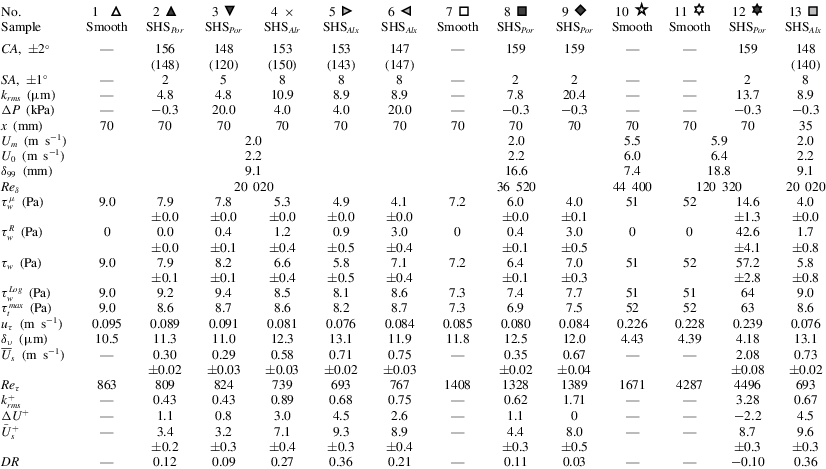
A summary of experimental conditions and measured parameters for all tests included in this paper. CA denotes the contact angle, SA the sliding angle and DR the drag reduction. Values of CA in parenthesis are contact angles measured after the experiment and exposing the wall to air. The same symbols apply for all the figures.
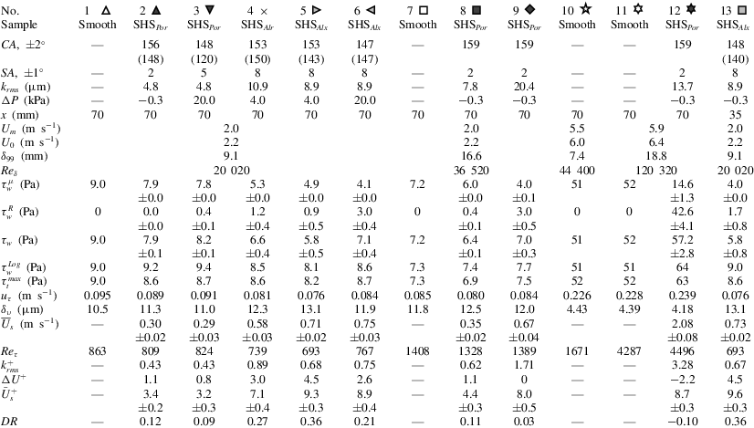
High-resolution velocity measurements have been performed for 20 cases, and results for 13 of them are included in this paper. As listed in table 1, they include
 $\text{SHS}_{Por}$
,
 $\text{SHS}_{Al}$
and smooth walls, with
 $U_{m}$
varying from 2 to
 $6~\text{m}~\text{s}^{-1}$
, pressure differences in the range
 $-0.3\leqslant {\rm\Delta}P\leqslant 20$
kPa, root mean square roughness height varying between
 $4.8\leqslant k_{rms}\leqslant 20.4~{\rm\mu}\text{m}$
and two streamwise locations. For control measurements above smooth walls, the SHSs are exchanged with smooth polyvinyl chloride bases and the measurement locations are kept identical as those of the SHSs. Table 1 also provides results of contact and sliding angle measurements performed before each experiment, which are denoted as CA and SA, respectively. The contact angle after the experiment and exposing the wall to air is also provided for some of the cases (in parenthesis). Each flow measurement is started after running the facility continuously at a particular condition for at least one hour. Each data acquisition lasts approximately two hours. We have also noticed that after running for more than four hours at
 $U_{m}=6.0~\text{m}~\text{s}^{-1}$
, the roughness height of the
 $\text{SHS}_{Por}$
decreases significantly, presumably due to mechanical degradation and entrainment of the sprayed polymer. For example, for case no. 12, the initial
 $k_{rms}$
value is
 $20.4~{\rm\mu}\text{m}$
, but after running for two hours at
 $U_{m}=6~\text{m}~\text{s}^{-1}$
prior to data acquisition,
 $k_{rms}$
decreases to
 $14.5~{\rm\mu}\text{m}$
. During the two hour data acquisition period, the values of
 $k_{rms}$
decrease from 14.5 to
 $13.7~{\rm\mu}\text{m}$
. Values measured at the end of the experiments are used in subsequent discussions. This phenomenon does not occur at
 $U_{m}=2.0~\text{m}~\text{s}^{-1}$
for both the
 $\text{SHS}_{Por}$
and/or the
 $\text{SHS}_{Al}$
.
Also listed in table 1 are the
 ${\it\tau}_{w}^{{\it\mu}}$
,
 ${\it\tau}_{w}^{R}$
,
 ${\it\tau}_{w}$
,
 $\overline{U}_{s}$
and their associated uncertainties. The values of
 $u_{{\it\tau}}=({\it\tau}_{w}/{\it\rho})^{1/2}$
and
 ${\it\delta}_{{\it\upsilon}}$
based on
 ${\it\tau}_{w}$
are provided in table 1. These values are used for the inner scaling. In the rest of the paper, a superscript
 $^{+}$
is used for quantities that are normalized by
 $u_{{\it\tau}}$
and
 ${\it\delta}_{{\it\upsilon}}$
, a subscript
 $_{0}$
for quantities measured above the smooth wall (the baseline) and the combination of the superscript
 $^{+}$
and subscript
 $_{0}$
for quantities normalized by
 $u_{{\it\tau}0}$
and
 ${\it\delta}_{{\it\upsilon}0}$
. For all cases, in addition to
 ${\it\tau}_{w}$
, we also estimate the wall friction by a logarithmic fit to the mean velocity profile in the regions where values of
 $y\partial \overline{U}/\partial y$
are nearly unchanged, which fall in the range of
 $80{\it\delta}_{{\it\upsilon}}<y<180{\it\delta}_{{\it\upsilon}}$
for cases no. 1 to no. 6 and no. 13,
 $50{\it\delta}_{{\it\upsilon}}<y<180{\it\delta}_{{\it\upsilon}}$
for cases no. 7 to no. 9 and
 $50{\it\delta}_{{\it\upsilon}}<y<350{\it\delta}_{{\it\upsilon}}$
for cases no. 10 to no. 12. Results, denoted as
 ${\it\tau}_{w}^{Log}$
, along with the maximum value of the total stress across the entire boundary layer, denoted as
 ${\it\tau}_{t}^{max}$
, are also listed in table 1. There are mismatches between the log layer based estimate of wall stress and the directly measured value. Implications of these findings are discussed later in this paper.
Because the high-resolution measurements only cover the inner part of the turbulent boundary layer, 2-D PIV has also been used to obtain the entire boundary profile, including the missing wake region. It has been performed at a lower magnification (
 $5.4~{\rm\mu}\text{m}~\text{pixel}^{-1}$
), using a larger sample area
 $(36\times 24~\text{mm}^{2},x\times y)$
. The centres of the sample areas (
 $x=70~\text{mm}$
) coincide with those of high-resolution measurements. These 2-D PIV measurements have also been performed after running at a particular experimental condition continuously for one hour. Data acquisitions typically last for 30 min, during which more than 250 pairs of images are captured. Standard PIV cross-correlations using in-house software (Roth & Katz Reference Roth and Katz2001) with a window size of
 $64{\it\delta}_{{\it\upsilon}}\times 16{\it\delta}_{{\it\upsilon}}$
(
 $x\times y$
) for
 $U_{m}=2~\text{m}~\text{s}^{-1},128{\it\delta}_{{\it\upsilon}}\times 32{\it\delta}_{{\it\upsilon}}$
(
 $x\times y$
) for
 $U_{m}=6~\text{m}~\text{s}^{-1}$
and 50 % overlap are used to calculate the velocity, resulting in a characteristic grid spacing of
 $32{\it\delta}_{{\it\upsilon}}\times 8{\it\delta}_{{\it\upsilon}}$
 $(x\times y)$
for
 $U_{m}=2~\text{m}~\text{s}^{-1}$
and
 $64{\it\delta}_{{\it\upsilon}}\times 16{\it\delta}_{{\it\upsilon}}$
(
 $x\times y$
) for
 $U_{m}=6~\text{m}~\text{s}^{-1}$
. The boundary layer thicknesses,
 ${\it\delta}_{99}$
, as listed in table 1, are based on the elevation where 99 % of the maximum velocity
 $(U_{0})$
is reached. Note that
 $U_{0}$
is slightly higher (typically by 8 %–12 %) than
 $U_{m}$
owing to the boundary layer-induced blockage. As is evident, unlike the total wall stress, the effects of the SHSs on
 ${\it\delta}_{99}$
are small, possibly since the present fetch
 $(4{-}9{\it\delta}_{99})$
is limited. The magnitudes of the drag reduction are defined as
 $DR=({\it\tau}_{w0}-{\it\tau}_{w})/{\it\tau}_{w0}$
, where
 ${\it\tau}_{w0}$
is the value obtained for the smooth wall at the same
 $U_{m}$
and very similar
 ${\it\delta}_{99}$
. To calculate the velocity deficit or increase in the log region,
 ${\rm\Delta}U^{+}$
, the mean velocity profile is fitted with
 $\overline{U}^{+}=(1/{\it\kappa})\ln y^{+}+{\rm\Delta}U^{+}+B_{0}$
, where
 $B_{0}$
is the value obtained for the corresponding smooth wall. For subsequent discussion, values of
 $Re_{{\it\delta}}=U_{0}{\it\delta}_{99}/{\it\upsilon}$
,
 $Re_{{\it\tau}}=u_{{\it\tau}}{\it\delta}_{99}/{\it\upsilon}$
,
 $k_{rms}^{+}$
,
 ${\rm\Delta}U^{+}$
,
 $\overline{U}_{s}^{+}$
and DR are also included in table 1. Note that when normalized,
 $\overline{U}_{s}^{+}={\it\lambda}_{x}^{+}$
for the cases where
 ${\it\tau}_{w}={\it\tau}_{w}^{{\it\mu}}$
, and
 $\overline{U}_{s}^{+}<{\it\lambda}_{x}^{+}$
for the cases where
 ${\it\tau}_{w}>{\it\tau}_{w}^{{\it\mu}}$
or
 ${\it\tau}_{w}^{R}>0$
.
Two facts need to be considered when comparing the presently measured wall friction to that of much larger surfaces. First, there is a relatively short distance (
 $4{-}9{\it\delta}_{99}$
) from the beginning of the SHSs to the sample area. Prior studies have reported an overshot of the wall friction after transitioning from a smooth to a rough wall and an undershot after transitioning from a rough to a smooth wall (Antonia & Luxton Reference Antonia and Luxton1971). Further downstream, the wall friction adjusts to the new boundary condition after a distance that increases with decreasing
 ${\it\delta}_{99}/k$
. For example, a relatively short distance of
 $2{-}3{\it\delta}_{99}$
is required for
 ${\it\delta}_{99}/k>1000$
(Saito & Pullin Reference Saito and Pullin2014), and a much longer distance of approximately
 $30{\it\delta}_{99}$
is needed for
 ${\it\delta}_{99}/k<25$
(Lee & Sung Reference Lee and Sung2007). If the roughness effects are dominant (as will be shown to occur in some cases), one would expect a rather quick transition considering
 ${\it\delta}_{99}/k_{rms}>100$
for current samples. There is limited information about the transition from a smooth wall to an SHS. However, a recent numerical study by Park (Reference Park2015) reports undershoots of the wall friction and adjustment distances to constant wall friction of
 $5{\it\delta}_{99}$
to
 $20{\it\delta}_{99}$
for SHSs with streamwise grooves of different wavelengths at
 $Re_{{\it\tau}}\sim 200$
. Most of the present measurements are performed at substantially higher Reynolds numbers and with random roughness. Moreover, due to this short distance, the outer region does not reach equilibrium condition, namely, the velocity profile in the log layer does not fully adjust to the local stress in the inner part of the boundary layer. For transition from a smooth to a rough wall, the required distance for mean velocity to be self-preserved varies from
 $10{\it\delta}_{99}$
to
 $40{\it\delta}_{99}$
(Saito & Pullin Reference Saito and Pullin2014). Overshoots of Reynolds stresses in this transition region have also been reported (Lee & Sung Reference Lee and Sung2007; Saito & Pullin Reference Saito and Pullin2014). Hence, in discussing the results, our main focus is on the inner region while highlighting discrepancies between the inner and outer regions. Furthermore, data are presented to demonstrate the streamwise evolution of the wall friction and Reynolds stresses in the outer part of the boundary layer. Second, without the plastron, the current SHSs fall in the transitionally rough to rough regimes (Schultz & Flack Reference Schultz and Flack2007) and form drag might affect the total stress at the spatially averaged top of the roughness elements. However, based on computational results found in Chan et al. (Reference Chan, Macdonald, Chung, Hutchins and Ooi2015), for a transitionally rough surface with
 $k^{+}=10$
, the total stress normalized by the wall friction near the roughness tip increases from approximately 0.87 to 0.97 as
 ${\it\delta}_{99}/k$
increases from 9 to 25. The viscous stress contributes approximately 60 % in both cases. In the current study, considering that
 ${\it\delta}_{99}/k_{rms}>100$
and
 $k_{rms}^{+}<5$
, it is reasonable to expect that the total stress near the roughness tip represents the wall friction.
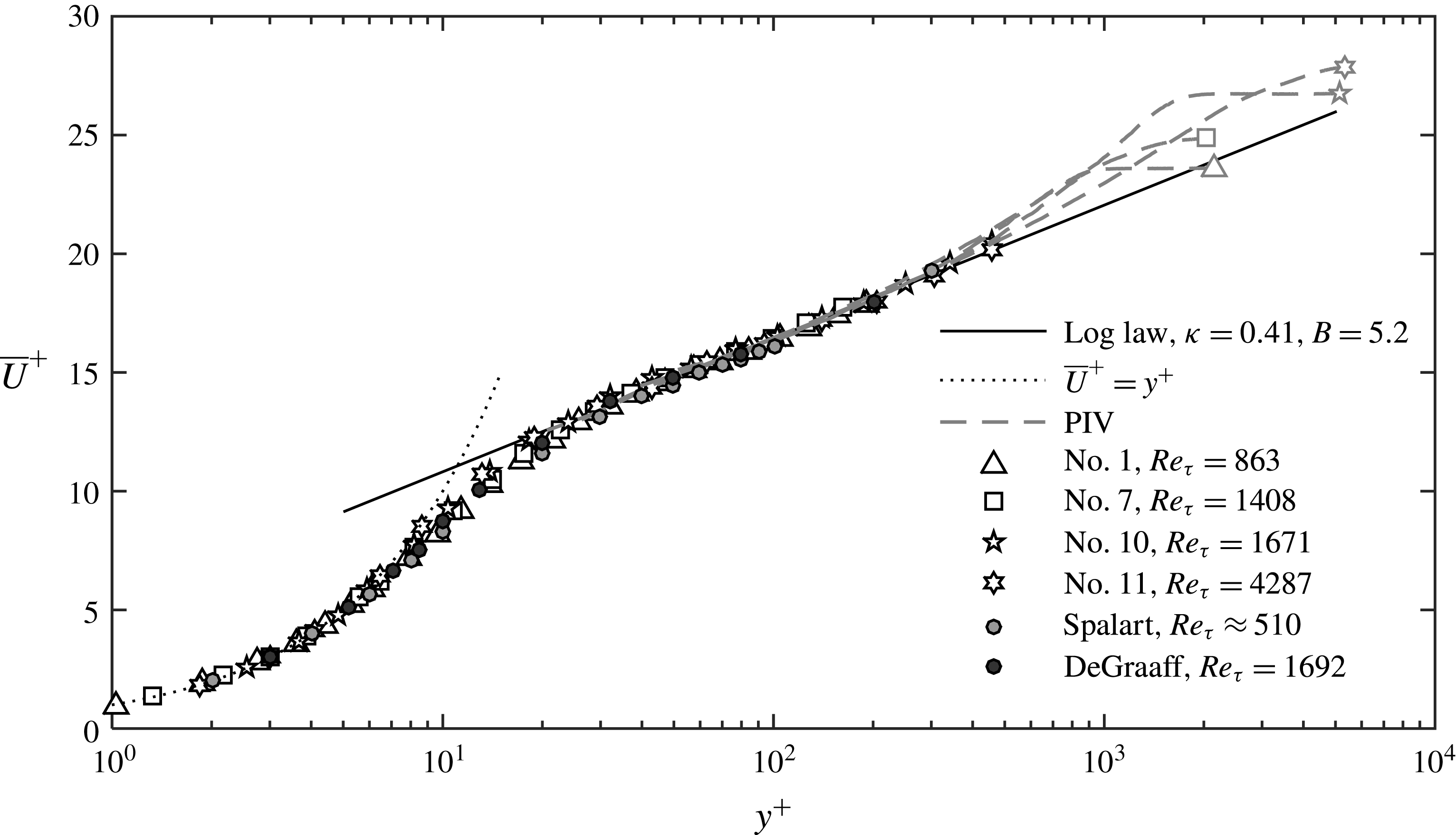
Mean velocity profiles for the baseline (smooth wall) cases. Symbols are consistent with those in table 1. Grey dashed lines and symbols are obtained from 2-D PIV and black symbols show DHM data.

3 Results
3.1 Mean flow quantities on smooth walls (baseline)
Data for smooth walls have been obtained as a baseline for comparison with the SHSs at the same location and free stream flow conditions. Wall stress results for four different values of
 $Re_{{\it\delta}}$
are summarized in table 1 (cases no. 1, no. 7, no. 10, no. 11). Due to differences in the inlet boundary conditions at the entrance to the test section imposed in the settling chamber, we achieve two different boundary layer characteristics. The first one is thinner, with
 ${\it\delta}_{99}=9.1~\text{mm}$
and 7.4 mm for
 $U_{m}=2.0~\text{m}~\text{s}^{-1}$
and
 $5.5~\text{m}~\text{s}^{-1}$
, respectively. The second one is thicker, with
 ${\it\delta}_{99}=16.6~\text{mm}$
and 18.8 mm for
 $U_{m}=2.0~\text{m}~\text{s}^{-1}$
and
 $5.9~\text{m}~\text{s}^{-1}$
, respectively. The corresponding values of
 ${\it\tau}_{w}$
and
 ${\it\delta}_{{\it\upsilon}}$
are also different. The latter falls in the
 $10\leqslant {\it\delta}_{{\it\upsilon}}\leqslant 12~{\rm\mu}\text{m}$
range for the low-speed measurements and
 ${\it\delta}_{{\it\upsilon}}\approx 4.4~{\rm\mu}\text{m}$
for the high-speed tests. The corresponding values of
 $Re_{{\it\tau}}$
vary from 863 to 4287. In all cases, the differences between the measured wall stress and the predictions based on fits to the log layer profiles are less than 2 %, further emphasizing the validity of the procedures used for calculating the stresses in this study. For comparison, results for similar values of
 $Re_{{\it\tau}}$
obtained in high-resolution Laser-Doppler Anemometer measurements by De Graaff & Eaton (Reference De Graaff and Eaton2000) and a DNS study by Spalart (Reference Spalart1988) are also included. Figure 5 shows all the normalized mean velocity profiles, including both high-resolution DHM and low-resolution PIV data. The DHM results collapse onto the classical law of the wall for the viscous sublayers (
 $y^{+}\leqslant 5$
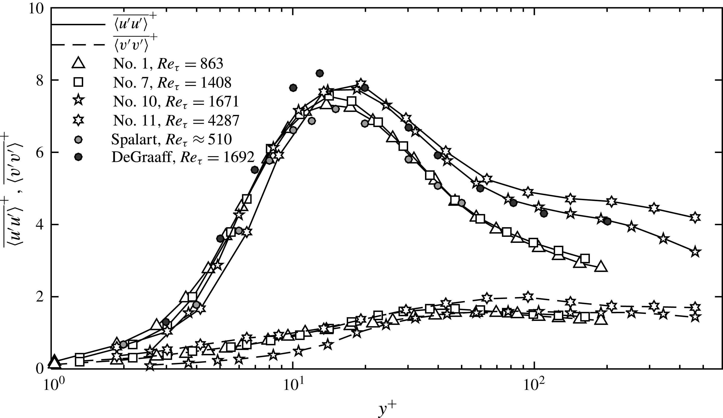
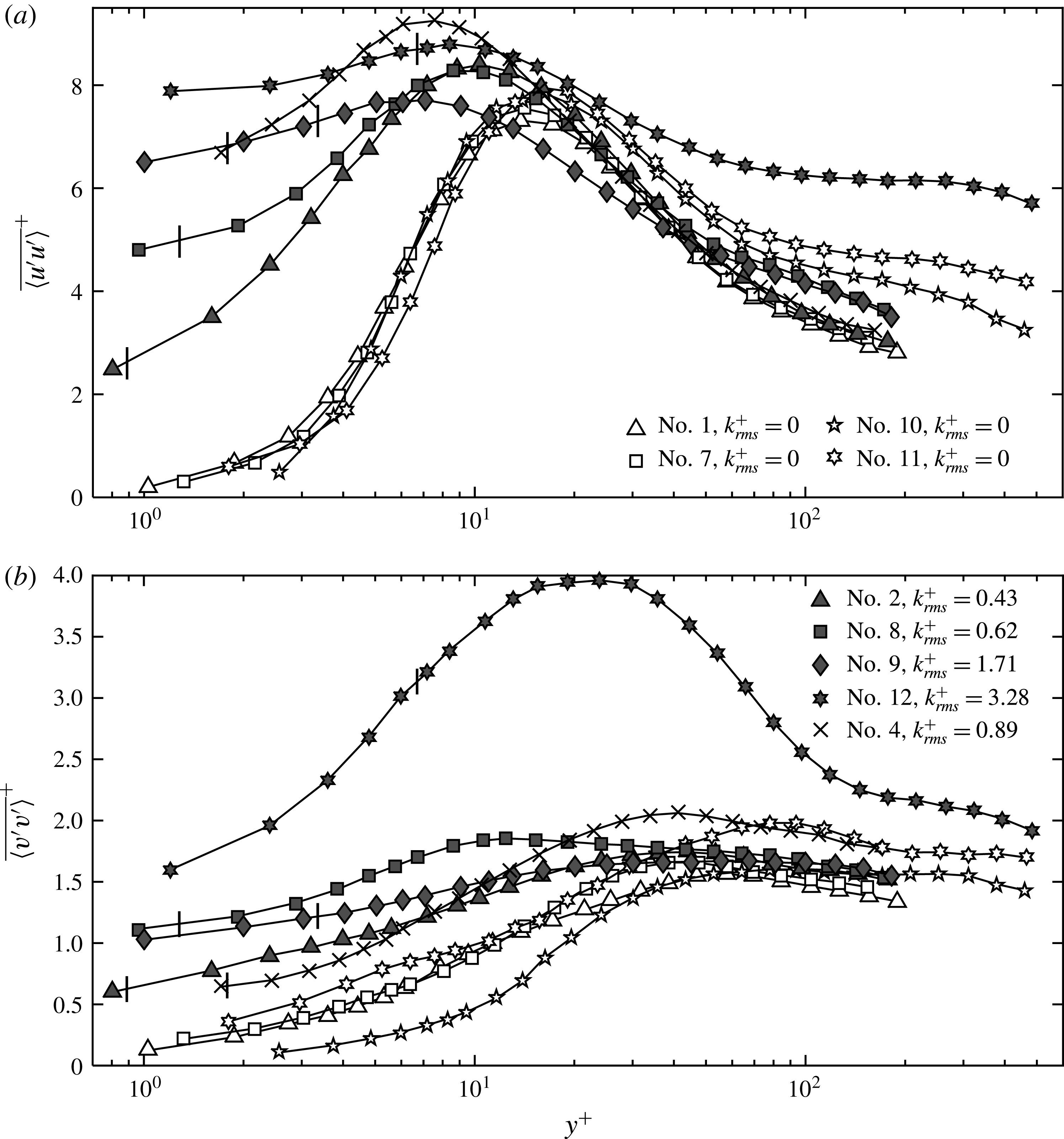
) and the familiar log-law for the log layers. The PIV data coincide with the DHM results in the log region, but extend to the wake and free stream flow. The results of Spalart (Reference Spalart1988) and De Graaff & Eaton (Reference De Graaff and Eaton2000) also collapse to the same profiles. In the rest of the paper, only DHM results will be shown. Figure 6 shows the streamwise and wall-normal velocity fluctuations. The present
 $\overline{\langle u^{\prime }u^{\prime }\rangle }^{+}$
profiles mostly coincide with the previously published boundary layer profiles at the corresponding
 $Re_{{\it\tau}}$
. The present peaks fall between the Spalart (Reference Spalart1988) and De Graaff & Eaton (Reference De Graaff and Eaton2000) values, i.e. slightly above the low
 $Re_{{\it\tau}}$
values of the former and slightly below the higher
 $Re_{{\it\tau}}$
results of the latter. As expected,
 $\overline{\langle u^{\prime }u^{\prime }\rangle }^{+}$
peaks in the
 $y^{+}=12{-}20$
range. The peak value increases with
 $Re_{{\it\tau}}$
, e.g. increase from 7 to 8 as increasing
 $Re_{{\it\tau}}$
from 500 to 2000. In the log layer,
 $\overline{\langle u^{\prime }u^{\prime }\rangle }$
increases with
 $Re_{{\it\tau}}$
, in agreement with Smits et al. (Reference Smits, McKeon and Marusic2011). The values of
 $\overline{\langle v^{\prime }v^{\prime }\rangle }$
reach a maximum of 1.6–1.9 at
 $y^{+}=50{-}100$
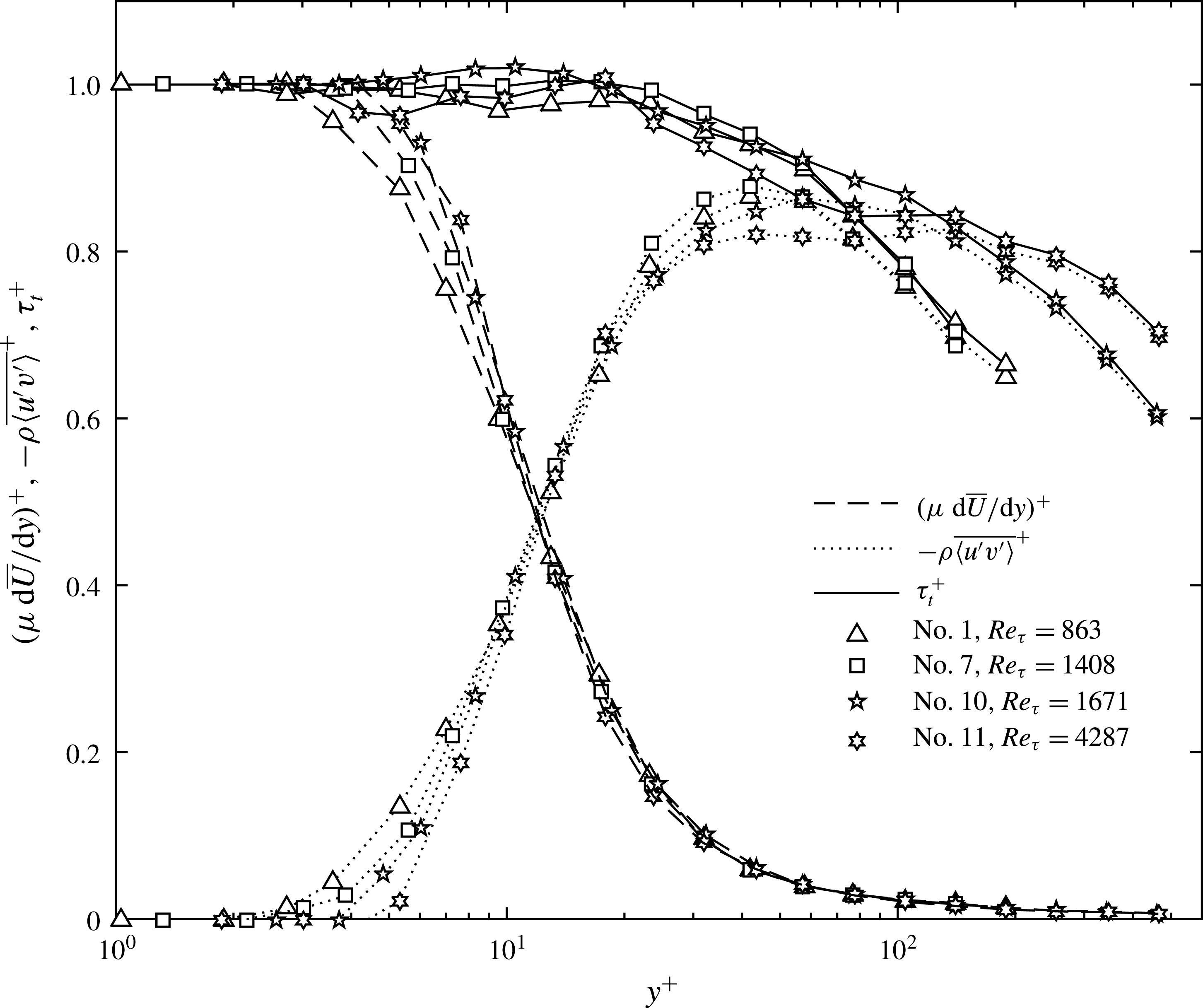
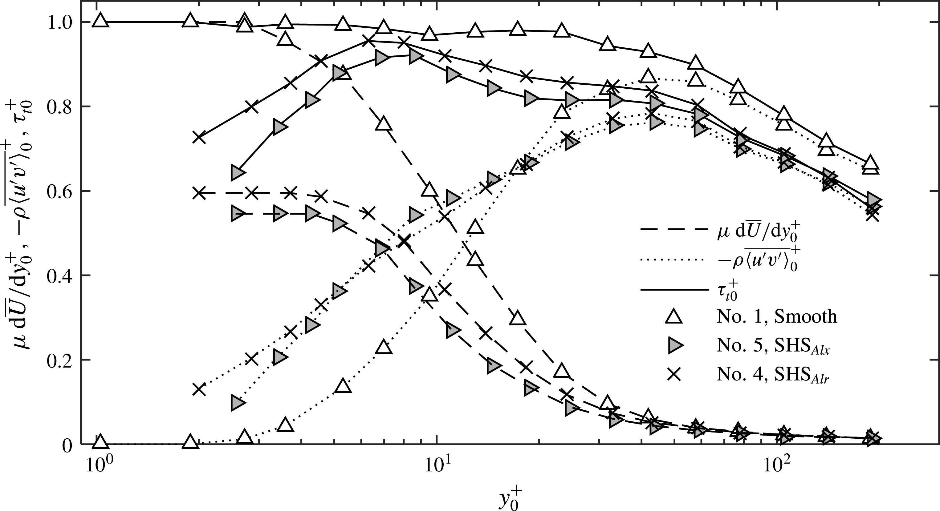
, again consistent with expectations. Figure 7 presents profiles of the viscous and Reynolds shear stresses along with the total stress. These results are also consistent with expectations, with the viscous stress decreasing monotonically and Reynolds shear stress increasing with elevation for
 $y^{+}<70$
, and then decreasing. For
 $y^{+}>70$
, the Reynolds shear stresses increases with increasing
 $Re_{{\it\tau}}$
. The total stress remains nearly constant up to about
 $y^{+}=20$
, and then starts decreasing at a rate that decreases with increasing
 $Re_{{\it\tau}}$
.
Baseline statistics of streamwise and wall-normal velocity fluctuations.

Profiles of baseline viscous shear stress (dashed lines), Reynolds shear stress (dotted lines) and total shear stress (solid lines).

Profiles of viscous shear stress for the
 $\text{SHS}_{Por}$
(grey symbols),
 $\text{SHS}_{Alr}$
(cross) and corresponding baseline cases (hollow symbols) for different values of
 $k_{rms}^{+}$
. Results are scaled by: (a) the smooth wall inner units and (b) their own inner units. The location of
 $y=2k_{rms}$
for each profile is marked by a short vertical line.

3.2 Effect of
 $k_{rms}^{+}$
and
$Re_{{\it\tau}}$
on the mean flow quantities for the
$\mathit{SHS}_{Por}$
and
$\mathit{SHS}_{Alr}$


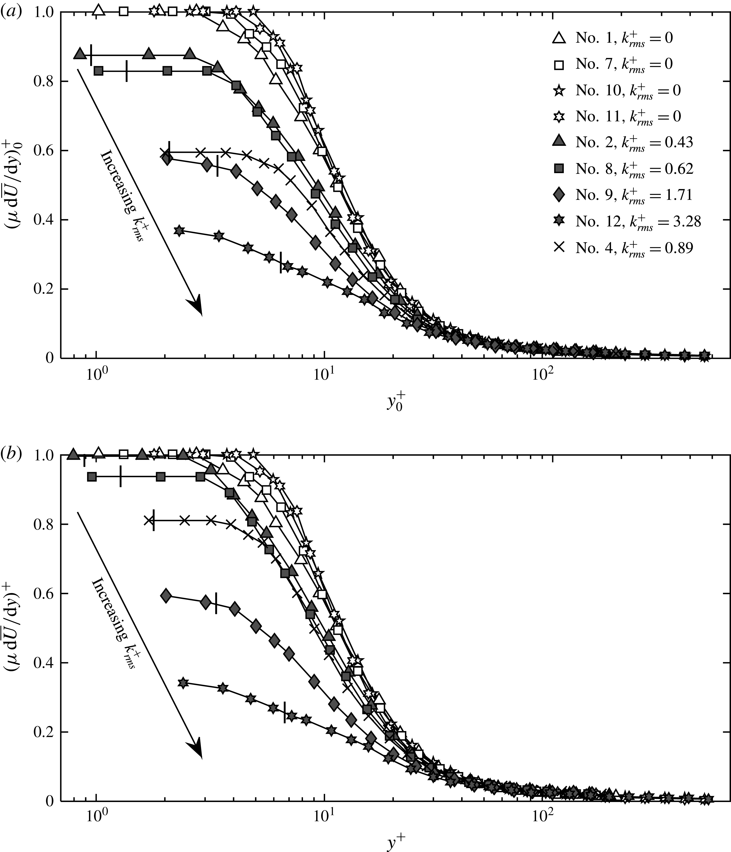
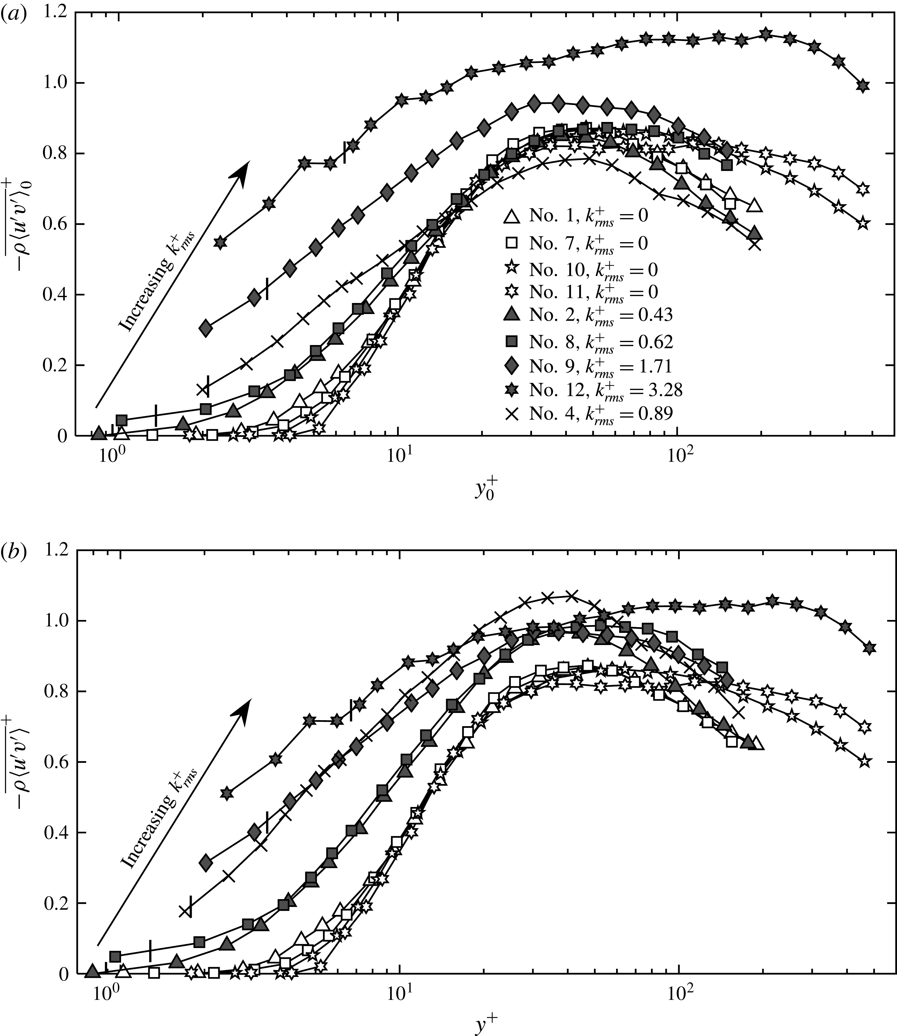
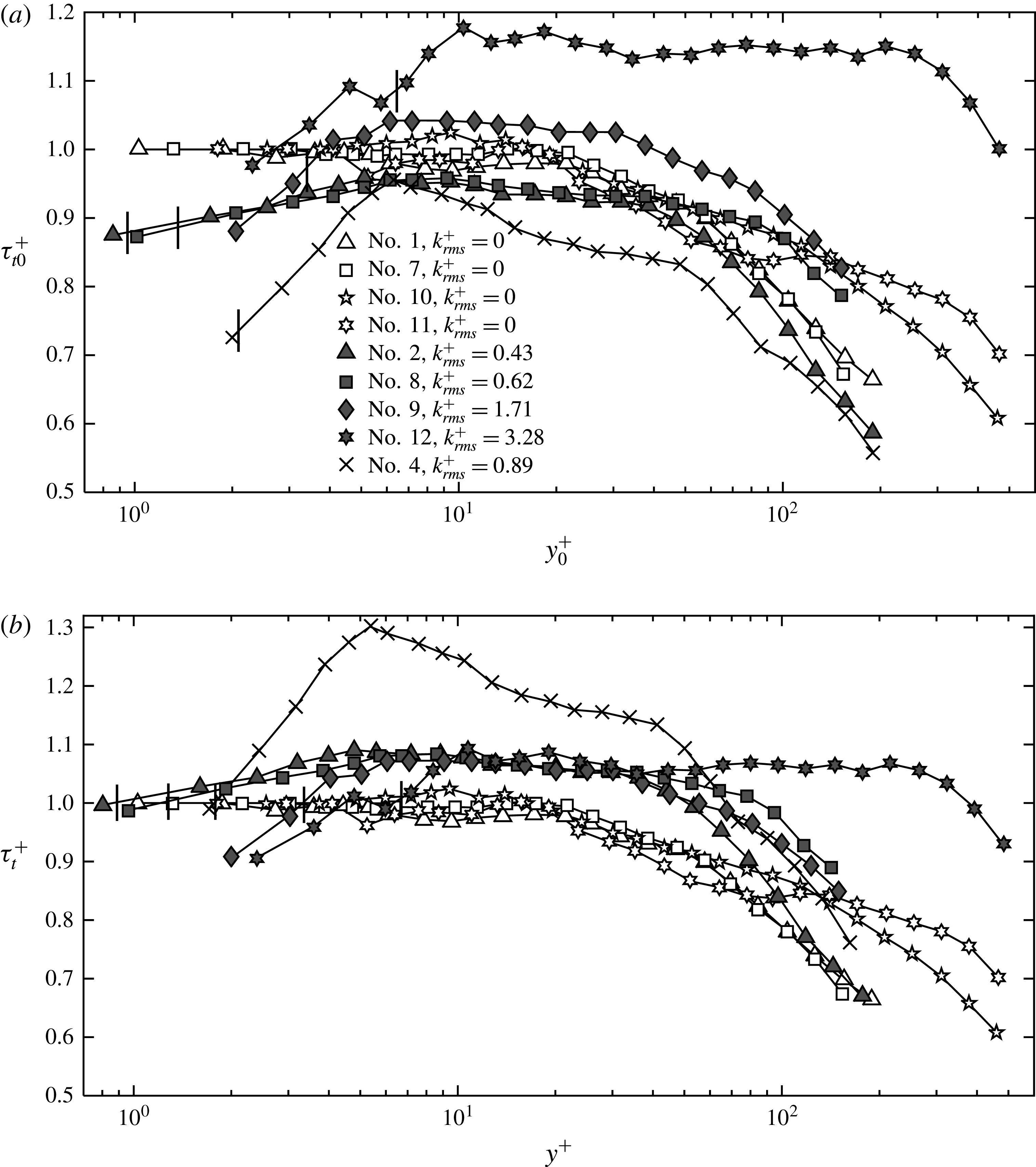
Profiles of viscous, Reynolds and total shear stresses for all the porous based sprayed surfaces, the etched aluminium surface and the smooth walls are shown in figures 8, 9 and 10, respectively. In each plot, the
 $\text{SHS}_{Por}$
results are presented using solid symbols, the
 $\text{SHS}_{Alr}$
data by crosses and the smooth wall profiles by hollow symbols. The specific flow conditions corresponding to each of the symbols can be found in table 1. The location of
 $y=2k_{rms}$
for each profile is marked by a short vertical line. Each profile is presented using two scales. In figures 8(a), 9(a) and 10(a), the results are scaled by the total wall stresses of the smooth walls for the same
 $U_{m}$
and very similar
 ${\it\delta}_{99}$
in order to highlight the differences from the smooth wall behaviour. In figures 8(b), 9(b) and 10(b), each profile is scaled by its own wall stress. Several trends are immediately evident. First, near the wall, the viscous stresses for all the SHSs are lower than those of the corresponding smooth wall values (for the same
 $U_{m}$
and
 ${\it\delta}_{99}$
). In the outer regions, the SHSs and smooth wall results collapse. Both values of
 ${\it\tau}_{w}^{{\it\mu}}/{\it\tau}_{w0}$
and
 ${\it\tau}_{w}^{{\it\mu}}/{\it\tau}_{w}$
decrease systematically with increasing
 $k_{rms}$
, but their magnitudes are inherently different. For the cases with skin friction reduction (cases with
 $k_{rms}^{+}<1$
),
 ${\it\tau}_{w}^{{\it\mu}}/{\it\tau}_{w0}$
is lower than
 ${\it\tau}_{w}^{{\it\mu}}/{\it\tau}_{w}$
. Conversely, for cases when the total wall stress increases (cases with
 $k_{rms}^{+}=3.28$
), the latter is lower. As expected for all the SHSs, the viscous stresses decrease with distance from the wall. In contrast, near the wall, Reynolds shear stresses for all the SHSs are larger than those of the corresponding smooth wall results (figure 9). Moreover, they are always non-zero at
 $y=2k_{rms}$
, and their magnitude increases with increasing
 $k_{rms}^{+}$
. Results for
 $k_{rms}^{+}=1.71$
and 3.28 are much higher than the rest. The locations and values of Reynolds shear stress maxima also depend on
 $k_{rms}^{+}$
. For
 $k_{rms}^{+}<1$
, the peaks normalized by
 ${\it\tau}_{w0}$
have values and locations that are very close to those of the corresponding smooth walls. The latter trend might be caused by the non-equilibrium conditions of the present boundary layers, as discussed further below. For
 $k_{rms}^{+}>1$
, the magnitudes are distinctly higher. When the Reynolds stresses are normalized by their own
 ${\it\tau}_{w}$
, the differences between peak values and their locations decrease, but all the SHSs peaks are consistently larger than those of the smooth walls. The total stresses on the SHSs also depend strongly on
 $k_{rms}^{+}$
. For all the
 $k_{rms}^{+}<1$
cases,
 ${\it\tau}_{w}/{\it\tau}_{w0}<1$
at
 $y=2k_{rms}$
, indicating a reduction of drag by these surfaces. The reduction is mild,
 ${\sim}10\,\%$
for the
 $\text{SHS}_{Por}$
, and above 25 % for the
 $\text{SHS}_{Alr}$
. For the
 $k_{rms}^{+}=1.71$
case,
 ${\it\tau}_{w}/{\it\tau}_{w0}$
(
 $y=2k_{rms}$
) is very close to 1, but for
 $k_{rms}^{+}=3.28$
,
 ${\it\tau}_{w}/{\it\tau}_{w0}$
is already significantly larger than 1. Considering that for the latter case,
 ${\it\tau}_{w}^{R}$
is the primary contributor to the total stress, it is clear that the surface roughness dominates the total drag. With increasing root mean square values of roughness height, the SHSs switch from facilitating drag reduction when
 $k_{rms}^{+}<1$
to increasing the drag for larger
 $k_{rms}^{+}$
. Similar trends are reported by Bidkar et al. (Reference Bidkar, Leblanc, Kulkarni, Bahadur, Ceccio and Perlin2014) based on force measurements of floating SHSs in a water tunnel. Their SHSs are generated by spray coating, cover a range of
 $k_{rms}^{+}$
ranging from 0.1 to 6 and show a maximum drag reduction of 30 % for
 $k_{rms}^{+}<0.5$
and an increase in drag for
 $k_{rms}^{+}>1$
. DNS results for textured surface by Busse & Sandham (Reference Busse and Sandham2013) also show similar trends.
Profiles of Reynolds shear stresses for the
 $\text{SHS}_{Por}$
(grey symbols),
 $\text{SHS}_{Alr}$
(cross) and corresponding baseline cases (hollow symbols) scaled by: (a) the smooth wall inner units and (b) their own inner units.

For the
 $\text{SHS}_{Por}$
, the values of
 ${\it\tau}_{t}^{+}$
collapse at
 $10<y^{+}<30$
, irrespective of roughness height (figure 10
b). They increase slightly with distance from the wall for
 $y^{+}\leqslant 2k_{rms}^{+}+5$
, peaking with values of approximately 1.05, and then remain nearly constant until
 $y^{+}=30$
, except for
 $k_{rms}^{+}=3.28$
, for which the constant stress layer persists up to
 $y^{+}=300$
. There is a persistent difference between the
 $\text{SHS}_{Por}$
and the smooth wall results in the constant stress region, suggesting that
 $\text{SHS}_{Por}$
boundary layers are under non-equilibrium conditions. The wall stresses of
 $\text{SHS}_{Por}$
are lower than those at higher elevation, presumably since the outer layers have not ‘relaxed’ yet from the smooth wall conditions. This claim is supported by the figure 10(a), which shows that, for
 $k_{rms}^{+}<1$
, i.e. the drag reduction cases, and at
 $5<y^{+}<10$
,
 ${\it\tau}_{w}/{\it\tau}_{w0}$
is nearly matched with the smooth wall values. The trends are very different for the rougher walls, presumably since turbulent mixing speeds up the momentum exchange between the inner and outer regions. The non-equilibrium conditions appear to be more severe for the
 $\text{SHS}_{Alr}$
, for which the drag reduction is significantly higher. Yet, its peak
 ${\it\tau}_{w}/{\it\tau}_{w0}$
is nearly the same as those of the smooth wall and
 $\text{SHS}_{Por}$
at
 $y^{+}=6$
, but it decreases sharply closer to the wall. At
 $6<y^{+}<100$
,
 ${\it\tau}_{w}/{\it\tau}_{w0}$
of the
 $\text{SHS}_{Alr}$
is lower than that of the other surfaces, but appears to collapse with the results for similar Reynolds numbers at higher elevations. Due to the lower wall stress, values of
 ${\it\tau}_{t}^{+}$
of the
 $\text{SHS}_{Alr}$
are much higher than the others in the inner part of the boundary layer, but the difference decreases in the outer regions. The mismatch between
 ${\it\tau}_{w}^{Log}$
and
 ${\it\tau}_{w}$
for all the SHSs is another way to show non-equilibrium conditions. As listed in table 1, for all the drag reduction cases, the values of
 ${\it\tau}_{w}^{Log}$
are larger than the corresponding
 ${\it\tau}_{w}$
and are very close to those of
 ${\it\tau}_{w0}$
for the same Reynolds number. This trend implies that the log region has not adjusted yet to the lower skin friction. Conversely, for the cases showing drag increase,
 ${\it\tau}_{w}^{Log}$
is noticeably larger than
 ${\it\tau}_{w0}$
, consistent with the previously argued effect of roughness-induced increase in wall-normal momentum exchange.

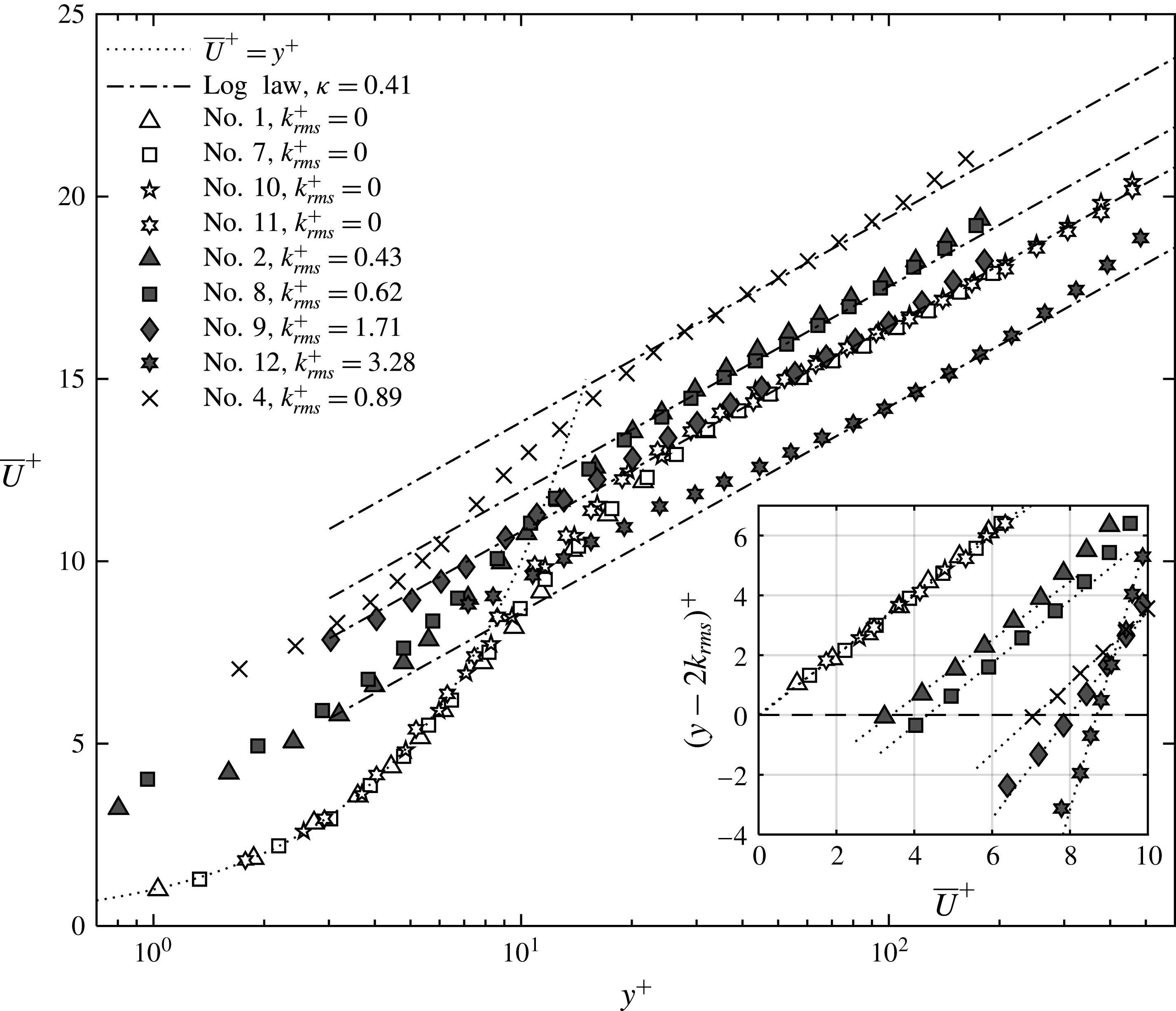
Using the same symbols, figure 11 shows the mean velocity profiles for the
 $\text{SHS}_{Por}$
,
 $\text{SHS}_{Alr}$
and the smooth walls scaled by their own inner units. The inset highlights the near-wall velocity profiles using a linear scale (with the axes switched), which allows direct comparison to linear least square fits. It confirms that for
 $k_{rms}^{+}<1$
, the inner profiles are nearly linear when
 $y^{+}\leqslant 5$
, but are slightly curved for
 $k_{rms}^{+}>1$
. For all the
 $k_{rms}^{+}<1$
, or drag reduction SHS cases, the mean velocity is higher than that of the smooth wall at all elevations, consistent with the numerical results by Min & Kim (Reference Min and Kim2004) and experimental measurements by Woolford et al. (Reference Woolford, Prince, Maynes and Webb2009). The upward shift in the log region is smaller than that occurring near the wall. There are two possible reasons for this difference. First, it might be influenced by the previously discussed non-equilibrium condition, i.e. that the log layer mean momentum has only partially adjusted to the lower wall friction. However, these differences have also been observed in DNS results obtained for equilibrium conditions, which Min & Kim (Reference Min and Kim2004) attribute to spanwise slip, which increases the skin friction by enhance the strength of streamwise vortices. In simulations prescribing only streamwise slip, i.e.
 ${\it\lambda}_{x}\neq 0$
and
 ${\it\lambda}_{z}=0$
, the upward shift in the velocity profile is uniform. Conversely, for the drag increase case (
 $k_{rms}^{+}=3.28$
), the log layer mean momentum is lower than that of the smooth wall. The entire profile resembles that measured over a rough wall, which is characterized by lower mean velocity gradients in the inner part of the boundary layer (Chan et al.
Reference Chan, Macdonald, Chung, Hutchins and Ooi2015). For
 $k_{rms}^{+}=1.71$
, the profile appears to be a transition from drag reduction to drag increase, with the inner region resembling a rough wall and a mild slope and the outer region in the process of crossing from the momentum increase to momentum decrease regimes.
Mean velocity profiles for the
 $\text{SHS}_{Por}$
(grey symbols),
 $\text{SHS}_{Alr}$
(cross) and baseline (white symbols) cases scaled by their own inner units. The inset shows the near-wall profiles in linear scales, with dotted lines indicating linear least square fits. Symbol legends are provided in table 1.

(a) Streamwise and (b) wall-normal velocity fluctuations normalized by their own inner units.

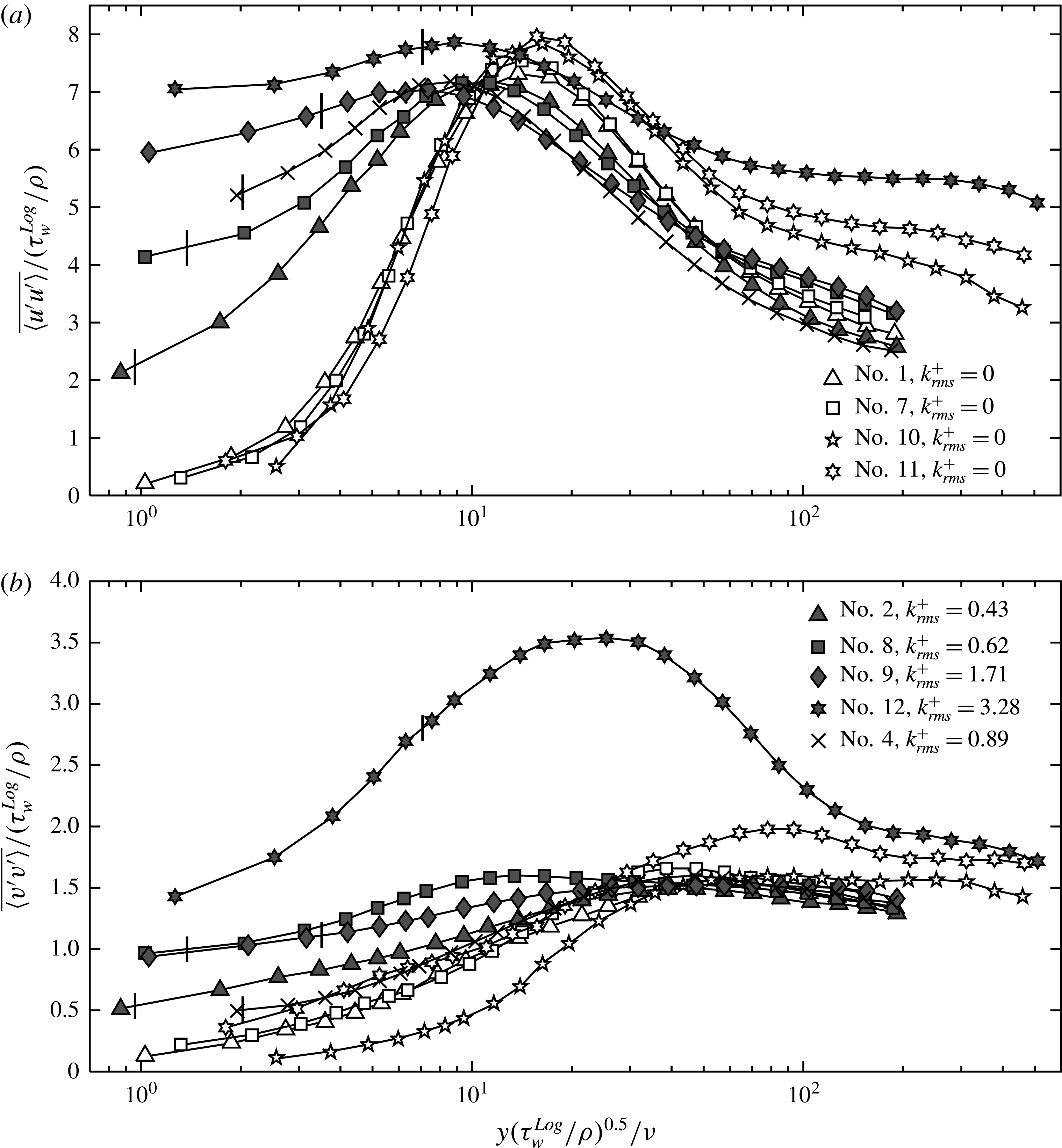
(a) Streamwise and (b) wall-normal velocity fluctuations normalized by shear stress estimated from a fit to the mean velocity in the log region.

Figures 12(a) and (b) present distributions of
 $\overline{\langle u^{\prime }u^{\prime }\rangle }$
and
 $\overline{\langle v^{\prime }v^{\prime }\rangle }$
, respectively. For all non-smooth wall cases, regardless of the magnitude of
 $k_{rms}^{+}$
, both
 $\overline{\langle u^{\prime }u^{\prime }\rangle }$
and
 $\overline{\langle v^{\prime }v^{\prime }\rangle }$
are significant in the vicinity of the roughness tips, and remain higher than the smooth wall values at
 $y^{+}<10$
. These trends are consistent with reported numerical results for SHSs (Busse & Sandham Reference Busse and Sandham2012). For the drag reduction cases (
 $k_{rms}^{+}<1$
),
 $\overline{\langle u^{\prime }u^{\prime }\rangle }^{+}$
increases with distance from the wall in the inner layer, peaks at
 $6<y^{+}\leqslant 10$
and then decreases at higher elevations, where it nearly collapses to the corresponding smooth wall data at
 $y^{+}>20$
. The peak values are slightly larger than those of the smooth wall by approximately 5 %, and are located closer to the wall. While the shift in location is consistent with the numerical results, the higher magnitude is not (Min & Kim Reference Min and Kim2004). There are several likely reasons for the discrepancy, such as roughness effects, motion of the air–water interface, spatial non-uniformity and even the non-equilibrium conditions. It should be noted that the actual magnitudes of the
 $\overline{\langle u^{\prime }u^{\prime }\rangle }$
peak for all the drag reduction cases are slightly lower than those of the corresponding smooth walls. Trends are quite different for the drag increase case (
 $k_{rms}^{+}=3.28$
), for which
 $\overline{\langle u^{\prime }u^{\prime }\rangle }^{+}$
flattens at
 $y^{+}<5$
. After having a broad maximum centred around
 $y^{+}\sim 9$
,
 $\overline{\langle u^{\prime }u^{\prime }\rangle }^{+}$
decreases but remains higher than that of the corresponding smooth walls. While previously published trends for transitionally rough walls show that in the inner region
 $\overline{\langle u^{\prime }u^{\prime }\rangle }^{+}$
can be higher or smaller than that of the smooth wall (Chan et al.
Reference Chan, Macdonald, Chung, Hutchins and Ooi2015), the present trends for the log layer are inconsistent with the expected collapse to the smooth wall data (Jimenez Reference Jimenez2004; Hong, Katz & Schultz Reference Hong, Katz and Schultz2011). The non-equilibrium condition appears to be a primary cause for this difference. Indeed, rescaling the
 $\overline{\langle u^{\prime }u^{\prime }\rangle }^{+}$
profile based on
 ${\it\tau}_{w}^{Log}$
substantially reduces the difference from the smooth wall results, as shown in figure 13(a). Furthermore, simulations of the transition from a smooth to a fully rough surface show overshoots of
 $\overline{\langle u^{\prime }u^{\prime }\rangle }^{+}$
in the log region (Saito & Pullin Reference Saito and Pullin2014). For the
 $k_{rms}^{+}=1.71$
case, at
 $y^{+}<5$
,
 $\overline{\langle u^{\prime }u^{\prime }\rangle }^{+}$
appears to have values and trends falling between those of the skin friction reduction and increase, but the broad peak appears at a lower elevation and has a lower magnitude than both. In the outer region, trends are similar to that of the
 $\text{SHS}_{Por}$
for the same Reynolds number.
For all the SHSs, the profiles of
 $\overline{\langle v^{\prime }v^{\prime }\rangle }^{+}$
have maximums in the
 $10<y^{+}<50$
range, closer to the wall than the smooth wall peaks. At
 $y^{+}>50$
, for the cases with mild drag reduction (
 $k_{rms}^{+}<1$
) and
 $k_{rms}^{+}=1.71$
, the values of
 $\overline{\langle v^{\prime }v^{\prime }\rangle }^{+}$
remain only slightly higher than those of the corresponding smooth wall. The difference is bigger for the
 $\text{SHS}_{Alr}$
, which causes more than 25 % drag reduction. Conversely, for the drag increase case (
 $k_{rms}^{+}=3.28$
), the values of
 $\overline{\langle v^{\prime }v^{\prime }\rangle }^{+}$
in the inner part of the boundary layer are substantially higher than those of the smooth wall. This difference diminishes but does not vanish in the log layer. Such an overshot of the peak value of
 $\overline{\langle v^{\prime }v^{\prime }\rangle }^{+}$
has been reported before for a boundary layer transitioning from a smooth to a rough wall, based on numerical simulations performed by Lee & Sung (Reference Lee and Sung2007) and by Saito & Pullin (Reference Saito and Pullin2014). Both indicate that the elevated values decay slowly, e.g. for more than 500 momentum thicknesses in the former study. When the
 $\overline{\langle v^{\prime }v^{\prime }\rangle }^{+}$
profiles are re-normalized based
 ${\it\tau}_{w}^{Log}$
, as shown in figure 13(b), the SHS profiles collapse to the smooth wall values at
 $y^{+}>20$
for
 $k_{rms}^{+}<2$
and at
 $y^{+}>100$
for the drag increase case (
 $k_{rms}^{+}=3.28$
). But the differences in the inner part of the boundary layer persist, especially for the drag increase case. Even under non-equilibrium conditions, trends of the outer parts of the evolving boundary layer in the rough wall case differ from those of the drag decrease cases. Both the rate at which the log layers response to the changing boundary conditions and the involved turbulence levels are different.
3.3 Effects of groove alignment, streamwise distance and pressure on the stress profiles
3.3.1 Groove alignment
The effects of the surface geometry are examined by comparing the shear stresses of the
 $\text{SHS}_{Alr}$
(randomly polished) and
 $\text{SHS}_{Alx}$
(streamwise polished) at the same location and for the same Reynolds number,
 ${\rm\Delta}P$
and
 $k_{rms}^{+}$
(table 1). Results are shown in figure 14. Both surfaces reduce the wall friction by more than 20 %. Although the magnitudes of the near-wall stresses are different, those differences are essentially limited to the near-wall region, and the profiles nearly collapse onto each other at higher elevations. At
 $y^{+}<5$
, both the viscous and Reynolds stresses above the
 $\text{SHS}_{Alx}$
are lower than those of
 $\text{SHS}_{Alr}$
, indicating that the axially aligned grooves are more effective in reducing drag. Accordingly, the slip velocity on the
 $\text{SHS}_{Alx}$
is also higher than that of
 $\text{SHS}_{Alr}$
as shown in table 1. As both
 $k_{rms}$
and contact angles are very similar, this difference might be associated with geometric differences, namely the
 ${\sim}110~{\rm\mu}\text{m}$
(
 ${\sim}8.5{\it\delta}_{{\it\upsilon}}$
) spaced streamwise grooves. Considering that the deeper (
 $5{-}15{\it\delta}_{{\it\upsilon}}$
) streamwise riblets have already been shown to reduce drag in turbulent boundary layers over rigid walls, e.g. by 10 % when the space of grooves is
 $15{\it\delta}_{{\it\upsilon}}$
(García-Mayoral & Jiménez Reference García-Mayoral and Jiménez2011), the groove alignment seems to play a role in the SHSs as well.
Effects of groove alignment on the etched aluminium surfaces on the viscous, Reynolds and total shear stresses scaled by smooth wall inner units.

3.3.2 Streamwise distance
The effects of streamwise distance from the transition between smooth to SHS have been evaluated by comparing the shear stresses on the
 $\text{SHS}_{Alx}$
at two locations,
 $x=3.9{\it\delta}_{99}$
and
 $7.7{\it\delta}_{99}$
, the latter being the location of most of the present tests. Several trends can be observed from the results presented in figure 15. Except for the first point, where results are essentially identical, the total stress at
 $x=3.9{\it\delta}_{99}$
and
 $y^{+}<40$
is slightly higher, by 10–15 %, than that further downstream, but the difference between them diminishes at higher elevations. This difference could be used as an estimate for non-equilibrium effects on the total stress. Trends of the two contributors to the total stress differ. At
 $y^{+}<8$
, the viscous stress at
 $x=3.9{\it\delta}_{99}$
is lower than that further downstream, but the profiles completely collapse at higher elevations. Conversely, the Reynolds shear stress at
 $x=3.9{\it\delta}_{99}$
is higher, and the difference between them slowly diminishes with increasing elevation, becoming very small at
 $y^{+}>40$
. For both contributors to the total stress, the profiles at
 $x=3.9{\it\delta}_{99}$
do not have intermediate values falling between the smooth wall and the more developed SHS further downstream. Such phenomena should be expected, as an overshoot in drag at the transition from smooth to rough walls (Saito & Pullin Reference Saito and Pullin2014) and an undershoot at the transition from rough to smooth walls (Antonia & Luxton Reference Antonia and Luxton1971) and from smooth wall to SHS (Park Reference Park2015) have been seen before. At the wall, the present results show an undershoot of viscous stress by 18 % and an overshoot of (very low) Reynolds shear stress by 88 %, both of which might be associated with the transitional effects.
Effects of streamwise distance on the viscous, Reynolds and total shear stresses.

3.3.3 Facility pressure
The effects of
 ${\rm\Delta}P$
are studied by comparing the stress profiles for the same
 $\text{SHS}_{Por}$
and the same
 $\text{SHS}_{Alx}$
under considerably different values of
 ${\rm\Delta}P$
. For the porous surfaces, the sign of
 ${\rm\Delta}P$
indicates the direction of air flow across the substrate, while for the
 $\text{SHS}_{Alx}$
, a sufficiently high
 ${\rm\Delta}P$
is expected to suppress the plastron that forms across the texture. To make results meaningful, the pressure is normalized by the surface tension, e.g. by
 ${\it\sigma}/k_{rms}$
. For the most of the porous surface tests,
 $-0.08\leqslant {\rm\Delta}Pk_{rms}/{\it\sigma}\leqslant -0.02$
, i.e. there is very slow air replenishment. Figure 16(a) compares the resulting profiles to those with
 ${\rm\Delta}Pk_{rms}/{\it\sigma}=1.33$
, i.e. when air replenishment is suppressed, while the pressure difference is of the same order as the surface tension. As is evident, increasing
 ${\rm\Delta}P$
does not have a detectable effect on the viscous stress, and slightly increases the Reynolds stress, resulting in a slight increase in the total stress while maintaining the drag reduction. It appears that under such pressure differences, the capillary forces are sufficient to maintain the air layer, as the hologram movies clearly show. In fact, under similar pressures, the drag reduction can only be suppressed by filling the chamber under the porous surface with water, and forcing it through the porous walls by the pressure difference. After doing this, the SHS is no longer super-hydrophobic, even after drying it. As for the etched aluminium SHSs, figure 16(b) compares the stress profiles for
 ${\rm\Delta}Pk_{rms}/{\it\sigma}=0.49$
and 2.47. As is evident and expected, suppressing the air layer causes a significant increase in the Reynolds and total stresses and a decrease of the viscous stress in the inner part of the boundary layer. Both trends are consistent with an increase in the ‘effective’ roughness height. Yet, the skin friction is still significantly lower than that of the smooth wall. Accordingly, the mean velocity profile at higher
 ${\rm\Delta}P$
is less upward shifted (not shown). The increasing role of the roughness with increasing
 ${\rm\Delta}P$
can also be observed from the distributions of the normal stresses shown in figure 16(c). Both the magnitudes of
 $\overline{\langle u^{\prime }u^{\prime }\rangle }_{0}^{+}$
and
 $\overline{\langle v^{\prime }v^{\prime }\rangle }_{0}^{+}$
increase with
 ${\rm\Delta}P$
over the entire inner part of the boundary layer, consistent with the trends presented in figures 12 and 13.
(a) Effects of pressure difference across the porous wall on the shear stresses above the
 $\text{SHS}_{Por}$
; and effects of facility pressure on (b) the shear stresses and (c) streamwise and wall-normal velocity fluctuations above the
 $\text{SHS}_{Alx}$
.

4 Discussion and conclusions
In this study, digital holographic microscopy is used for characterizing the profiles of mean velocity, viscous and Reynolds shear stresses, as well as turbulence level in the inner part of turbulent boundary layers over several super-hydrophobic surfaces. Two types of SHSs are involved, namely
 $\text{SHS}_{Por}$
generated by spray coating hydrophobic material on porous bases and
 $\text{SHS}_{Al}$
created by using vapour deposition to coat etched solid aluminium bases. The magnitudes of
 $Re_{{\it\tau}}$
range from 693 to 4496 and
 $k_{rms}^{+}$
vary from 0.43 to 3.28. Experiments are also repeated at different streamwise locations and ambient pressures as well as with aluminium surfaces that are either polished randomly or along the streamwise direction. The wall shear stress is estimated from the sum of the viscous and Reynolds shear stress at the top of roughness elements, and the mean slip velocity is obtained from the mean profile at the same elevation.
The data show that the near-wall momentum transport involves a competition between two opposing effects, namely skin friction reduction by the SHSs, and an increase in Reynolds stresses with increasing roughness effects. Their relative significance depends on the values of
 $k_{rms}^{+}$
. As
 $k_{rms}^{+}$
increases from 0.43 to 3.28, the near-wall stresses transition from drag reduction, when the viscous stress dominates, to drag increase when the Reynolds shear stress is the primary contributor. For
 $k_{rms}^{+}<1$
, the SHSs cause a reduction of drag as well as an upward shift of the mean velocity profiles. In the log region, this upward shift is lower than that in the inner layer, a phenomenon observed before in both numerical simulations (e.g. Min & Kim Reference Min and Kim2004) and experimental measurements (e.g. Woolford et al.
Reference Woolford, Prince, Maynes and Webb2009). These changes are accompanied with increases in
 $\overline{\langle u^{\prime }u^{\prime }\rangle }^{+}$
and
 $\overline{\langle v^{\prime }v^{\prime }\rangle }^{+}$
, the latter only slightly, in the inner part of the boundary layer, and shifts of their peaks closer to the wall. Roughness effects, motion of the air–water interface, spatial non-uniformity and even the non-equilibrium conditions might play a role in the increase of the turbulence level. When
 $k_{rms}^{+}=1.71$
, it appears that there is a balance between drag reduction by the SHS and an increase by the roughness. For
 $k_{rms}^{+}=3.28$
, the roughness becomes dominant, causing an increase in wall friction, a downward shift in the mean velocity profile and increases in
 $\overline{\langle u^{\prime }u^{\prime }\rangle }^{+}$
and
 $\overline{\langle v^{\prime }v^{\prime }\rangle }^{+}$
close to the wall. Consistent with prior experimental studies involving measurements of wall friction (Bidkar et al.
Reference Bidkar, Leblanc, Kulkarni, Bahadur, Ceccio and Perlin2014), it appears that the transition between drag reduction to increase occurs when
 $k_{rms}$
falls in the
 $1\leqslant k_{rms}^{+}\leqslant 2$
range. This observation should presumably refer to the height of roughness elements extending above the air layer. This transition might be affected by roughness spacing and gas fraction, which are not measured in the present study.
Due to limited total length of the SHSs,
 $8{-}20{\it\delta}_{99}$
, all the present boundary layers do not reach equilibrium conditions. Hence, for the drag reduction cases, the directly measured local wall stress is lower than that calculated from a fit to the mean velocity profile in the log layer. The latter decreases gradually from the smooth wall value to that of the SHS as the boundary layer develops with streamwise distance. The evolving conditions also introduce wall-normal gradients in the total stress profiles, with the near-wall values being lower than the maximum values at the edge of the roughness/viscous sublayers. This maximum also decreases with streamwise distance. Collapse of the normal and shear Reynolds stress components onto those of the smooth wall in the outer part of the log layer is also consistent with the boundary being under non-equilibrium conditions. There is also a mismatch between the local wall stress and that estimated from a log layer fit to the velocity profile for cases where roughness effects dominate. However, in these cases, the log fitted values are higher than both the local values and those of the smooth wall. Furthermore, all the Reynolds stress components and the total stress in the log region are much higher than those of the smooth wall. These observations are consistent to recent results of numerical simulations, which also observe an overshoot of the velocity fluctuation in the log region shortly after a transition from a smooth to a rough wall (Lee & Sung Reference Lee and Sung2007; Saito & Pullin Reference Saito and Pullin2014). Clearly, the changing boundary conditions propagate in the wall-normal direction much faster above the rough wall than the SHS which reduces drag.
Symbols (table 1) show the measured drag reduction as a function of dimensionless slip velocity in comparison to theoretical prediction (lines) based on (1.2), using the empirical values of
 $F({\it\lambda}_{z}^{+})$
of Busse & Sandham (Reference Busse and Sandham2012). Circles show DNS results by Park et al. (Reference Park, Park and Kim2013a
) for broadly spaced streamwise grooves.

Several other effects have also been observed. First, increasing the pressure in the facility to
 ${\rm\Delta}Pk_{rms}/{\it\sigma}>1$
appears to suppress the air layer, and presumably exposes the roughness elements to the liquid. Hence, the turbulence level and the shear stress in the inner part of the boundary layer increase. As one would expect, the effect of pressure on drag reduction cannot be ignored. Second, for the etched aluminium surfaces, aligning the surface groves in the streamwise direction causes higher drag reduction than a randomly polished surface. Finally, we conclude this paper by discussing the relationship between slip velocity, based on values measured at the top of the roughness and the drag reduction for all the present SHSs. Figure 17 is a plot of DR versus
 $\overline{U}_{s}^{+}$
, where each case is represented by the symbols listed in table 1 and used throughout this paper. It also shows the theoretical predictions by Busse & Sandham (Reference Busse and Sandham2012), based on (1.2) and the empirical function
 $F({\it\lambda}_{z}^{+})=16/(4+{\it\lambda}_{z}^{+})-1$
. The model results are provided for two relevant values of
 $Re_{{\it\tau}}$
, both for
 ${\it\lambda}_{z}=0$
and
 ${\it\lambda}_{z}={\it\lambda}_{x}$
. However, for the experimental data,
 ${\it\lambda}_{x}^{+}$
is replaced by
 $\overline{U}_{s}^{+}$
at the top of the roughness. That means that we assume that the present measurements are equivalent to a hypothetical case for which the air layer surface is aligned with the top of the roughness, and the viscous stress there is equal to the total stress. As discussed before,
 $\overline{U}_{s}^{+}\leqslant {\it\lambda}_{x}^{+}$
and the equal sign is only valid when
 ${\it\tau}_{w}^{R}=0$
. As discussed in Busse & Sandham (Reference Busse and Sandham2012), the introduction of spanwise slip and an increase in
 $Re_{{\it\tau}}$
reduces the extent of drag reduction. The
 ${\it\lambda}_{z}=0$
case predictions agree with the DNS results of Park et al. (Reference Park, Park and Kim2013a
) for an SHS consisting of long and broadly spaced streamwise grooves, which presumably involve limited spanwise slip. However, as is evident, except for the
 ${\rm\Delta}Pk_{rms}/{\it\sigma}=2.47$
test, all of the present cases that involve drag reduction fall close to the predicted values assuming
 ${\it\lambda}_{z}^{+}={\it\lambda}_{x}^{+}$
. While not surprising for the randomly distributed roughness, it raises questions for the
 $\text{SHS}_{Alx}$
results, where the non-uniformly distributed grooves are preferentially aligned in the streamwise direction. It is difficult to assess why
 $\text{SHS}_{Alx}$
gives a drag reduction and slip length that are higher than those of the randomly aligned
 $\text{SHS}_{Alr}$
, but still fall on the
 ${\it\lambda}_{z}^{+}={\it\lambda}_{x}^{+}$
curve. If the streamwise slip is preferentially higher, one would expect that the drag reduction would also fall above the
 ${\it\lambda}_{z}^{+}={\it\lambda}_{x}^{+}$
curve. There are several possible reasons for this trend, such as effects of the non-uniform spacing, which may allow some spanwise slips and/or roughness effects, as evidenced by the elevated Reynolds stress at the top of the grooves (figure 14). We have not performed measurements using other groove spacings or depths, so the significance of this observation remains unclear. Only three experimental cases deviate significantly from the predicted values, all of which involve an increasing role of roughness. Two of them are the
 $k_{rms}^{+}=1.71$
and 3.28 cases and the third is the
 $\text{SHS}_{Alx}$
with
 ${\rm\Delta}Pk_{rms}/{\it\sigma}=2.47$
, namely when the plastron is partially suppressed (the drag is still lower than the smooth wall value) by increasing the pressure in the test facility. Hence, for situations where the roughness effect is not dominant, i.e. the Reynolds stress at the top of the roughness is much lower than the viscous stress, the present measurements confirm the theoretical relationship between drag reduction and slip length for a turbulent boundary layer over an SHS. To the best of our knowledge, the present study provides the first simultaneous direct measurement of both slip velocity and drag reduction, allowing such a comparison.
Acknowledgements
This research has been performed under the ONR MURI program on Passive and Active Friction Drag Reduction of Turbulent Flows over Super-Hydrophobic Surfaces led by S. Ceccio. The program officer is K.-H. Kim. The authors also thank S. King and Y. Ronzhes for their assistance in setting up the experiments, and J. Wang for developing the GPU-based hologram reconstruction code.
Supplementary movies
Supplementary movies are available at http://dx.doi.org/10.1017/jfm.2016.450.