





1. Introduction
The study of magnetised plasmas is of crucial importance in applications such as fusion energy, space weather and astrophysics. Numerical simulations provide an effective way of studying plasma behaviour, by avoiding the prohibitive costs of conducting in situ and remote measurements. The large variation in length and time scales in the dynamics of magnetised plasmas poses a challenge for numerical methods and computer simulations (Stix Reference Stix1992; Brambilla Reference Brambilla1998; Fitzpatrick Reference Fitzpatrick2022). To capture the diverse range of phenomena observed in magnetised plasmas, researchers have proposed numerous physical models over the years, with various numerical techniques based on these models. These models are broadly divided into three categories: kinetic models that describe the full velocity-space distribution function of each species; fluid models assuming a near-Maxwellian distribution and, therefore, allowing the plasma to be characterised by moments of the distribution function such as density, temperature and bulk velocity; and hybrid models that are a combination of the other two. Kinetic models are used when kinetic effects such as non-Maxwellian distributions, wave–particle interactions and kinetic instabilities become important. They employ the Vlasov equation in combination with Maxwell’s laws of electromagnetism to describe the dynamics of the plasma. When the physical dimensions of the problem studied are much larger (>
 ${\sim}20$
times) than the Debye length, the plasma can be considered as being quasineutral across these length scales, i.e. having an equal number of positive and negative charge carriers. Quasineutral models filter out the lower length scales over which charge separation phenomena occur. They also remove the description of high-frequency electromagnetic wave propagation from the Vlasov–Maxwell system. Quasineutral models are therefore reduced models that eliminate the need for resolving these small time and length scales, resulting in faster numerical schemes and more efficient use of computational resources.
Numerical algorithms for quasineutral systems have been developed over the years and still remain an active area of research in computational plasma physics. Joyce et al. (Reference Joyce, Lampe, Slinker and Manheimer1997) developed an electrostatic PIC technique for quasineutral plasmas wherein the electric field was obtained directly from the momentum equation and the quasineutrality condition, rather than the Poisson equation. Cheng & Johnson (Reference Cheng and Johnson1999) introduced a kinetic-fluid model wherein multiple ion species were modelled as a single fluid and kinetic effects were incorporated through plasma pressure tensors that were computed from particle distribution functions obtained by solving the Vlasov or gyrokinetic equation. Crispel, Degond & Vignal (Reference Crispel, Degond and Vignal2005) developed numerical models for the quasineutral limit of a two-fluid, isentropic Euler–Poisson system. They later proposed for this system an improved, asymptotic-preserving (AP) scheme that was less restricted in terms of temporal and spatial discretisation (Crispel, Degond & Vignal Reference Crispel, Degond and Vignal2007). Degond, Deluzet & Navoret (Reference Degond, Deluzet and Navoret2006) introduced the first asymptotically stable PIC scheme for the near-quasineutral Vlasov–Poisson system for electrostatic, collisionless plasmas. They later made this scheme fully asymptotic-preserving and extended its stability to larger time steps (Degond et al. Reference Degond, Deluzet, Navoret, Sun and Vignal2010). Degond et al. then also developed AP schemes for fluid-like models such as the Euler–Maxwell model (Degond et al. Reference Degond, Deluzet and Savelief2012a ) and hybrid systems like the Euler–Poisson–Boltzmann equations (Degond et al. Reference Degond, Liu, Savelief and Vignal2012b ), in the quasineutral limit. Finally, they developed AP PIC methods for the quasineutral Vlasov–Maxwell model, allowing for fully electromagnetic plasma simulations with significant magnetic fields (Degond, Deluzet & Doyen Reference Degond, Deluzet and Doyen2017). For a detailed review and comparison of these asymptotic schemes, the reader is referred to the work by Degond & Deluzet (Reference Degond and Deluzet2017).
There has also been a considerable amount of work done in the plasma physics community on methods that preserve certain geometric structures of the physical system of equations being solved. These structures could be divergences, gauge invariances or conservation laws, for instance. For example, energy-conserving PIC discretisations of the electrostatic Vlasov–Poisson (Lewis Reference Lewis1970) and electromagnetic Vlasov–Maxwell (Lewis Reference Lewis1972) systems were developed that used a leapfrog time-integrator. These early works on structure-preserving methods used finite-differences for discretising fields. Markidis & Lapenta (Reference Markidis and Lapenta2011) proposed a fully discrete energy-conserving semi-implicit PIC scheme based on the implicit midpoint discretisation of Maxwell’s equations. Lapenta (Reference Lapenta2017) then reduced the computational cost of this method by removing the need for the nonlinear iterative solution procedure, while still maintaining discrete energy conservation. Chen, Chacón & Barnes (Reference Chen, Chacón and Barnes2011) proposed an energy-conserving fully implicit discretisation for the electrostatic Vlasov–Poisson system. Chen & Chacon (Reference Chen and Chacon2015) developed a nonlinearly implicit electromagnetic PIC algorithm based on the Vlasov–Darwin model that exactly conserves both total energy and charge through a consistent field–particle coupling. However, these energy-conserving implicit schemes are not derived from a variational or Hamiltonian principle and, therefore, do not preserve the de Rham or Poisson structure of the Vlasov–Maxwell system. Methods that rely on the de Rham structure of the Maxwell equations were also being developed for PIC methods that used finite-element meshes (Bossavit Reference Bossavit1998; Hiptmair Reference Hiptmair2002). These ensured an exact preservation of the discretised version of the Gauss laws. Tronci et al. (Reference Tronci, Tassi, Camporeale and Morrison2014) investigated the conservation properties of the Hamiltonian structures of some quasineutral hybrid Vlasov–MHD models. More recently, a geometric electromagnetic PIC (GEMPIC) method that used finite elements was developed, based on the Vlasov–Maxwell system’s intrinsic Hamiltonian structure (Kraus et al. Reference Kraus, Kormann, Morrison and Sonnendrücker2017; Campos Pinto et al. Reference Campos Pinto, Kormann and Sonnendrücker2022). Techniques from finite element exterior calculus (FEEC) (Arnold Reference Arnold2018) were employed, which conserved discretised versions of the Gauss laws, total energy, the Poisson structure and Casimir invariants.
In addition to finite elements, this approach has now also been developed with a discretisation based on structure-preserving mimetic finite differences (Kormann & Sonnendrücker Reference Kormann and Sonnendrücker2024). These mimetic discretisations employ operators that exactly imitate vector calculus identities on discrete spaces (Bochev & Hyman Reference Bochev and Hyman2006). To achieve this, unknowns are represented as point values, edge integrals, face integrals and volume integrals, constituting a discrete de Rham complex. Recently, this approach has also been extended to the drift-kinetic (DK) model and the hybrid model with drift electrons and kinetic ions by Meng et al. (Reference Meng, Kormann, Poulsen and Sonnendrücker2025). In this work, we aim to extend this method to the quasineutral limit of the Vlasov–Maxwell PIC system with both kinetic electrons and ions. We start with the Lagrangian from Tronci & Camporeale (Reference Tronci and Camporeale2015) and then propose a discretised Lagrangian based on the geometric structure-preserving discretisation related to mimetic finite differences. Importantly, our approach is derived directly in the quasineutral limit, rather than relying on asymptotic consistency of a full Vlasov–Maxwell solver upon the Debye length approaching zero, as in the work by Degond et al. (Reference Degond, Deluzet and Doyen2017). Because the formulation is derived directly in the quasineutral limit, the scheme ensures the absence of electromagnetic and Langmuir waves in the numerical solution. In contrast, asymptotic-preserving approaches rely on numerical damping to get rid of these waves in the quasineutral limit as the Debye length tends to zero. Another important feature of our model is that the discretised field equations and equations of motion for particles are both derived from the discretised Lagrangian, ensuring structure preservation in the semi-discretised space. At the semi-discrete level, we show that this system preserves the sum of the magnetic and kinetic energies, and maintains the zero-divergence requirement of the current density for the quasineutral model. We then check the wave spectra of single- and double-species quasineutral plasmas to verify our numerical model, using quasi-one-dimensional (quasi-1-D) test cases with periodic boundary conditions. A wave-damping simulation with periodic boundary conditions is also conducted to verify the theoretically predicted damping rate obtained from the dispersion relation.
The organisation of this paper is as follows. Section 2 describes the quasineutral, fully kinetic Vlasov–Maxwell model, including the governing equations, action principle and the electric field equation. Section 3 describes the spaces and discretisation used for describing the fields. Section 4 describes the splines used for the coupling between particles and fields. Section 5 details the space-discretisation for the governing equations derived from the discrete action principle, the semi-discretised electric field equation and energy-conserving properties. Section 6 details the time-stepping algorithm used to solve the discretised quasineutral system. The dispersion relation and various waves obtained are described in § 7. Numerical tests with periodic boundary conditions used to validate the framework and scaling studies are detailed in § 8. Finally, § 9 summarises our findings and provides general conclusions.
2. The quasineutral Vlasov–Maxwell model
2.1. Governing equations
In a fully kinetic model of a plasma, a species
 $s$
is described using a phase-space distribution function
 $f_s$
that is a function of space (
 $\boldsymbol{x}$
), velocity (
 $\boldsymbol{v}$
) and time (
 $t$
). This function
 $f_s$
evolves according to the Vlasov equation given by
 \begin{align} \frac {\partial f_s}{\partial t} + \boldsymbol{v} \boldsymbol{\cdot }\boldsymbol{\nabla} _x f_s + \frac {q_s}{m_s}{(\boldsymbol{E} + \boldsymbol{v} \times \boldsymbol{B})} \boldsymbol{\cdot }\boldsymbol{\nabla} _v f_s=0, \end{align}
where
 $q_s$
and
 $m_s$
are the particle charge and mass for the species
 $s$
, and
 $\boldsymbol{E}$
and
 $\boldsymbol{B}$
are the electric and magnetic fields. Here, (
 $\boldsymbol{X}$
) and (
 $\boldsymbol{V}$
) are characteristics of the Vlasov equation. In the quasineutral model, the electric and magnetic fields satisfy the following Maxwell equations:
 \begin{align} \boldsymbol{\nabla }\times \boldsymbol{B} = \mu _0 \boldsymbol{J}, \end{align}
 \begin{align} \frac {\partial \boldsymbol{B}}{\partial t} + \boldsymbol{\nabla }\times \boldsymbol{E} = \textbf {0}, \end{align}
 \begin{align} \rho = 0, \end{align}
 \begin{align} \boldsymbol{\nabla }\boldsymbol{\cdot }\boldsymbol{B} = 0. \end{align}
Here,
 $\mu _0$
is the magnetic permeability of vacuum. Equations (2.1)–(2.5) together comprise the Vlasov–Maxwell system in the quasineutral limit. The charge density,
 $\rho$
, and the current density,
 $\boldsymbol{J}$
, are obtained by integrating the zeroth and first moments of the distribution function
 $f_s$
over the velocity space:
 \begin{align} \rho = \sum _{s} q_s \int f_s \text{d}\boldsymbol{v}, \end{align}
 \begin{align} \boldsymbol{J} = \sum _{s} q_s \int f_s \boldsymbol{v} \text{d}\boldsymbol{v}. \end{align}
In the full Vlasov–Maxwell system, without taking the quasineutral limit, the Ampère equation i.e. (2.2), also contains the displacement current term given by
 $({1}/{c^2}) ({\partial \boldsymbol{E}}/{\partial t})$
, which can also be written as
 $\mu _0 \epsilon _0 ({\partial \boldsymbol{E}}/{\partial t})$
. Here,
 $c$
is the speed of light and
 $\epsilon _0$
is the permittivity of vacuum. In the full system, (2.4) becomes
 $\rho = \epsilon _0 \boldsymbol{\nabla }\boldsymbol{\cdot }\boldsymbol{E}$
. The quasineutral model is obtained by taking the formal limit
 $\epsilon _0 \to 0$
, thus leading to the previous equations. Integrating the Vlasov equation (2.1) over the velocity space and using the
 $\rho = 0$
condition from (2.4) gives the divergence-free condition for the current density:
 \begin{align} \boldsymbol{\nabla }\boldsymbol{\cdot }\boldsymbol{J} = 0. \end{align}
The magnetic field can be written in terms of the magnetic vector potential
 $\boldsymbol{A}$
as
 \begin{align} \boldsymbol{B} = \boldsymbol{\nabla }\times \boldsymbol{A}. \end{align}
Ampère’s equation (2.2) then can be written as
 \begin{align} \boldsymbol{\nabla }\times \boldsymbol{\nabla }\times \boldsymbol{A} = \boldsymbol{\nabla }(\boldsymbol{\nabla }\boldsymbol{\cdot }\boldsymbol{A}) - \boldsymbol{\nabla} ^2\boldsymbol{A} = \mu _0 \boldsymbol{J}. \end{align}
The quasineutrality condition,
 $\boldsymbol{\nabla }\boldsymbol{\cdot }\boldsymbol{J} = 0$
, makes it convenient to use the Coulomb gauge condition
 \begin{align} \boldsymbol{\nabla }\boldsymbol{\cdot }\boldsymbol{A} = 0. \end{align}
This further simplifies (2.10) to the Laplace equation
 \begin{align} - \boldsymbol{\nabla} ^2\boldsymbol{A} = \mu _0 \boldsymbol{J}. \end{align}
We note that the use of periodic boundary conditions in the test cases considered here allows a straightforward imposition of the Coulomb gauge condition in (2.11). This in turn allows the curl–curl operator to be reduced to a Laplace operator that is invertible up to an additional constant. Non-periodic boundary conditions would introduce the need for additional constraints on
 $\boldsymbol{A}$
at domain boundaries that are consistent with the Coulomb gauge.
2.2. Action principle
To obtain the previous governing equations in the continuous form, we start from the action principle developed by Tronci & Camporeale (Reference Tronci and Camporeale2015), which reads
 \begin{align} L(\boldsymbol{A}(t),\phi (t), \boldsymbol{X}_s(t),\dot {\boldsymbol{X}_s}(t),\boldsymbol{V}_s(t)) = \sum _s\int \bigg((m_s \boldsymbol{V}_s(t) + q_s\boldsymbol{A}(t,\boldsymbol{X}_s(t))) \boldsymbol{\cdot }\dot {\boldsymbol{X}_s}(t) \nonumber \\ - \frac 12 m_s V_s^2- q_s \phi (t,\boldsymbol{X}_s(t))\bigg) f_{s,0}\, \mathrm{d} \boldsymbol{x}_0\, \mathrm{d} \boldsymbol{v}_0 - \int \frac {1}{2\mu _0} \left | \boldsymbol{\nabla }\times \boldsymbol{A}(t,\boldsymbol{x})\right |^2 \,\mathrm{d} \boldsymbol{x}, \end{align}
where
 $\boldsymbol{E} = - ({\partial \boldsymbol{A}}/{\partial t}) - \boldsymbol{\nabla }\phi$
and
 $\boldsymbol{B} = \boldsymbol{\nabla }\times \boldsymbol{A}$
. The sum is over all particle species.
Remark 1.
In principle, the constraint
 $\boldsymbol{\nabla }\boldsymbol{\cdot }\boldsymbol{J}=0$
follows from
 $\boldsymbol{\nabla }\times \boldsymbol{B} = \boldsymbol{J}$
, but we will not be able to enforce this exactly numerically. For this reason, we need to enforce it with a Lagrange multiplier which will yield a slight modification of the electric field used for pushing the particles, so that the divergence of the current generated by the particles stays 0.
The physical system can be derived from this action. The variations with respect to
 $\boldsymbol{X}_s$
and
 $\boldsymbol{V}_s$
yield the Euler–Lagrange equations for the particles,
 $( {\partial }/{\partial t}) ({\partial L}/{\partial \dot {\boldsymbol{X}}}) = ( {\partial L}/{\partial \boldsymbol{X}})$
and
 $({\partial L}/{\partial \boldsymbol{V}} )= \textbf {0}$
. In this case, they become
 \begin{align} \frac {\mathrm{d} \boldsymbol{X}_s}{\mathrm{d} t} =\boldsymbol{V}_s, \end{align}
 \begin{align} \frac {\mathrm{d} \boldsymbol{V}_s}{\mathrm{d} t} = \frac {q_s}{m_s}( \boldsymbol{E} + \boldsymbol{V}_s\times \boldsymbol{B}). \end{align}
The solutions of (2.14) and (2.15) are the characteristic equations of the Vlasov equation. Taking the total derivative of
 $f_s$
, and using (2.14)–(2.15), gives the Vlasov equation for
 $f_s$
.
However, the variations in
 $\boldsymbol{A}$
yield
 \begin{align} \int \boldsymbol{B} \boldsymbol{\cdot }\boldsymbol{\nabla }\times \delta {\boldsymbol{A}} \mathrm{d} \boldsymbol{x} = \sum _s q_s \int \delta {\boldsymbol{A}} \boldsymbol{\cdot }\boldsymbol{v} f\, \mathrm{d}\boldsymbol{x} \,\mathrm{d}\boldsymbol{v} \quad \forall \delta {\boldsymbol{A}}, \end{align}
which becomes in strong form
 \begin{align} \boldsymbol{\nabla }\times \boldsymbol{B} = \mu _0\boldsymbol{J} = \mu _0 \sum _s\boldsymbol{J}_s = \mu _0 \sum _s q_s \int f_s \boldsymbol{v} \,\mathrm{d} \boldsymbol{v}. \end{align}
The variations in
 $\phi$
yield
 \begin{align} \sum _s q_s \int \delta {\phi } f_s\, \mathrm{d}\boldsymbol{x}\, \mathrm{d}\boldsymbol{v} = 0 \quad \forall \delta {\phi } ,\end{align}
which is the quasineutrality condition
 \begin{align} \rho = \sum _s q_s \int f_s\, \mathrm{d}\boldsymbol{v} = 0. \end{align}
Equation (2.19) also implies
 $\boldsymbol{\nabla }\boldsymbol{\cdot }\boldsymbol{J} = 0$
because of the continuity equation (2.8). Moreover, Faraday’s equation (2.3) follows directly from the definition of the fields from the potentials. Similarly, the Gauss law for magnetism (2.5) follows from the definition of the magnetic field.
2.3. Electric field equation
In the quasineutral model, without the displacement current
 $({1}/{c^2}) ({\partial \boldsymbol{E}}/{\partial t})$
in Ampère’s equation, the electric field cannot be evolved using its time derivative. An equation is therefore required to obtain the electric field at any time instant. Taking the curl of (2.3) and the time derivative of (2.2), and combining the two equations, we obtain
 \begin{align} \boldsymbol{\nabla }\times \boldsymbol{\nabla }\times \boldsymbol{E} = - \mu _0 \frac {\partial \boldsymbol{J}}{\partial t}. \end{align}
Next, multiplying the Vlasov equation by
 $q_s\boldsymbol{v}$
and integrating over the velocity space, we obtain
 \begin{align} \frac {\partial \boldsymbol{J}}{\partial t} = \sum _s\frac {\partial \boldsymbol{J}_s}{\partial t} = \sum _s \frac {q_s}{m_s} (\rho _s\boldsymbol{E} + \boldsymbol{J}_s \times \boldsymbol{B} - \boldsymbol{\nabla }\boldsymbol{\cdot }\mathbb{S}_s), \end{align}
where
 $\rho _s$
,
 $\boldsymbol{J}_s$
and
 $\mathbb{S}_s$
are the contributions of species
 $s$
to the charge density, current density and stress tensor, given by
 \begin{align} \rho _s = q_s \int f_s \text{d}\boldsymbol{v}, \end{align}
 \begin{align} \boldsymbol{J}_s = q_s \int f_s \boldsymbol{v} \text{d}\boldsymbol{v}, \end{align}
 \begin{align} \mathbb{S}_s = m_s \int f_s \boldsymbol{v} \otimes \boldsymbol{v} \text{d}\boldsymbol{v}. \end{align}
Substituting (2.21) in (2.20) gives the following equation for the electric field:
 \begin{align} \boldsymbol{\nabla }\times \boldsymbol{\nabla }\times \boldsymbol{E} + \mu _0 \sum _s \frac {q_s}{m_s}\rho _s\boldsymbol{E} = \mu _0\sum _s \frac {q_s}{m_s} (-\boldsymbol{J}_s \times \boldsymbol{B} + \boldsymbol{\nabla }\boldsymbol{\cdot }\mathbb{S}_s). \end{align}
This equation can be solved at every time step to obtain the electric field. It must be noted that we also have the option to solve (2.20) to obtain
 $\boldsymbol{E}$
. However, in the discrete setting, this would require the use of a time discretisation scheme to obtain the discrete
 $( {\partial \boldsymbol{J}}/{\partial t})$
. The electric field solution would depend on the discrete derivative used, which is not the case for (2.25). More importantly, the system in (2.20) is singular due to the curl–curl term. However, (2.25) is non-singular and determinate on account of the
 $\sum\nolimits_s ( {q_s}/{m_s})\rho _s\boldsymbol{E}$
term on the left-hand side. The left-hand side of (2.25) results in a symmetric, positive definite matrix after discretisation, making it straightforward to solve.
3. Spatial discretisation of fields
We use a dual-grid approach for the spatial discretisation of our model, wherein the dual or adjoint grid vertices are the barycentres of the primal grid cells. The numerical values for the field variables are located on spaces based on points, edges, faces and volumes of hexahedral (3-D) or quadrilateral (2-D) cells. This discretisation, based on mimetic finite differences, has already been used in GEMPICX for discretising the fully kinetic (Kormann & Sonnendrücker Reference Kormann and Sonnendrücker2024) and the drift-kinetic (Meng et al. Reference Meng, Kormann, Poulsen and Sonnendrücker2025) Vlasov–Maxwell models. The nodal, edge, face and volume spaces on the primal grids are denoted by
 $\mathcal{C}_0$
,
 $\mathcal{C}_1$
,
 $\mathcal{C}_2$
and
 $\mathcal{C}_3$
, respectively. Similarly, those on the dual grids are denoted by
 $\tilde {\mathcal{C}}_0$
,
 $\tilde {\mathcal{C}}_1$
,
 $\tilde {\mathcal{C}}_2$
and
 $\tilde {\mathcal{C}}_3$
, respectively. A duality exists between the primal and dual spaces. The nodes, edges, faces and cell volumes on the primal grid are each uniquely associated with the cell volumes, faces, edges and nodes on the dual grid, respectively. On the primal grid, the electric field
 $\boldsymbol{E}$
and the vector potential
 $\boldsymbol{A}$
are defined as edge-integrals and the magnetic field
 $\boldsymbol{B}$
is defined as face-integrals. On the dual grid, the magnetic field intensity
 $\boldsymbol{H}$
is defined as edge-integrals, the current density
 $\boldsymbol{J}$
and electric field intensity
 $\boldsymbol{D}$
are defined as face-integrals, and the charge density
 $\rho$
is defined as volume-integrals. Such an approach allows for exact preservation of certain discretised quantities. For example, the discrete divergence of
 $\boldsymbol{J}$
becomes a volume-integral on the dual grid, which is the same space where the charge density
 $\rho$
is defined. These spaces are shown in figure 1 for the primal grid.
Spaces for defining discrete variables on a primal Cartesian grid.

Figure 1. Long description
A diagram of a cell complex showing the structure of different dimensional cells. Panel A: A grid of points representing 0-cells. Panel B: Lines connecting the points representing 1-cells. Panel C: Faces formed by the lines representing 2-cells. Panel D: Cubes formed by the faces representing 3-cells.
3.1. Reduction operators
The reduction operators, also called restriction operators, relate a continuous field to its discretised counterparts defined on nodes, edges, faces and volumes. On the primal grid, these are as follows.
-
(i)
 $\mathcal{R}_0$
relates a scalar field to its values at primal grid nodes:(3.1)Here,
\begin{align} \mathcal{R}_0(\psi )_{i,j,k} = \psi (x_i, y_j, z_k) = {\boldsymbol{\psi }}_{i,j,k}. \end{align}
$\boldsymbol{\psi } \in \mathcal{C}_0$
.
-
(ii)
$\mathcal{R}_1$
relates a vector field to its integrals on primal grid edges:(3.2)
\begin{align} \mathcal{R}_1^x(E_x)_{i,j,k} = \int _{x_i}^{x_{i+1}} E_x(x, y_j, z_k)\, \mathrm{d} x = {{\boldsymbol{\mathsf{E}}}}_{i+1/2,j,k} = {{\boldsymbol{\mathsf{E}}}}^x_{i,j,k}, \end{align}
(3.3)
\begin{align} \mathcal{R}_1^y(E_y)_{i,j,k} = \int _{y_j}^{y_{j+1}} E_y(x_i, y, z_k)\, \mathrm{d} y = {{\boldsymbol{\mathsf{E}}}}_{i,j+1/2,k} = {{\boldsymbol{\mathsf{E}}}}^y_{i,j,k}, \end{align}
(3.4)Here,
\begin{align} \mathcal{R}_1^z(E_z)_{i,j,k} = \int _{z_k}^{z_{k+1}} E_z(x_i, y_j, z)\, \mathrm{d} z = {{\boldsymbol{\mathsf{E}}}}_{i,j,k+1/2} = {{\boldsymbol{\mathsf{E}}}}^z_{i,j,k}. \end{align}
$\mathcal{R}_1(\boldsymbol{E}) = (\mathcal{R}_1^x(E_x), \mathcal{R}_1^y(E_y), \mathcal{R}_1^z(E_z)) = ({{\boldsymbol{\mathsf{E}}}}^x,{{\boldsymbol{\mathsf{E}}}}^y,{{\boldsymbol{\mathsf{E}}}}^z)$
and
${\boldsymbol{\mathsf{E}}} = ({\boldsymbol{\mathsf{E}}}^x, {\boldsymbol{\mathsf{E}}}^y, {\boldsymbol{\mathsf{E}}}^z) \in \mathcal{C}_1$
.
-
(iii)
$\mathcal{R}_2$
relates a vector field to its integrals on primal grid faces:(3.5)
\begin{align} \mathcal{R}_2^x(B_x)_{i,j,k} = \int _{z_k}^{z_{k+1}} \int _{y_j}^{y_{j+1}} B_x(x_i, y, z)\, \mathrm{d} y\,\mathrm{d} z = {{\boldsymbol{\mathsf{B}}}}_{i,j+1/2,k+1/2} = {{\boldsymbol{\mathsf{B}}}}^x_{i,j,k}, \end{align}
(3.6)
\begin{align} \mathcal{R}_2^y(B_y)_{i,j,k} = \int _{z_k}^{z_{k+1}} \int _{x_i}^{x_{i+1}} B_y(x, y_j, z)\, \mathrm{d} x\,\mathrm{d} z = {{\boldsymbol{\mathsf{B}}}}_{i+1/2,j,k+1/2} = {{\boldsymbol{\mathsf{B}}}}^y_{i,j,k}, \end{align}
(3.7)Here,
\begin{align} \mathcal{R}_2^z(B_z)_{i,j,k} = \int _{y_j}^{y_{j+1}} \int _{x_i}^{x_{i+1}} B_z(x, y, z_k)\, \mathrm{d} x\,\mathrm{d} y = {{\boldsymbol{\mathsf{B}}}}_{i+1/2,j+1/2,k} = {{\boldsymbol{\mathsf{B}}}}^z_{i,j,k}. \end{align}
$\mathcal{R}_2(\boldsymbol{B}) = (\mathcal{R}_2^x(B_x), \mathcal{R}_2^y(B_y), \mathcal{R}_2^z(B_z)) = ({{\boldsymbol{\mathsf{B}}}}^x,{{\boldsymbol{\mathsf{B}}}}^y,{{\boldsymbol{\mathsf{B}}}}^z)$
and
${\boldsymbol{\mathsf{B}}} = ({\boldsymbol{\mathsf{B}}}^x, {\boldsymbol{\mathsf{B}}}^y, {\boldsymbol{\mathsf{B}}}^z) \in \mathcal{C}_2$
.
-
(iv)
$\mathcal{R}_3$
relates a scalar field to its volume integrals over primal grid cells:(3.8)Here,
\begin{align} \mathcal{R}_3(\rho )_{i,j,k} = \int _{z_k}^{z_{k+1}} \int _{y_j}^{y_{j+1}} \int _{x_i}^{x_{i+1}} \rho (x, y, z)\, \mathrm{d} x\,\mathrm{d} y\,\mathrm{d} z = {\boldsymbol{\rho }}_{i,j,k}. \end{align}
$\boldsymbol{\rho } \in \mathcal{C}_3$
.


The reduction/restriction operators on the dual mesh are similarly defined as follows.
-
(i)
$\tilde {\mathcal{R}}_0$
relates a scalar field to its values at dual grid nodes:(3.9)Here,
\begin{align} \tilde {\mathcal{R}}_0(\phi )_{i,j,k} = \phi (x_{i+1/2}, y_{j+1/2}, z_{k+1/2}) = \,\tilde {\!\boldsymbol{\phi }}_{i+1/2,j+1/2,k+1/2}. \end{align}
$\,\tilde {\!\boldsymbol{\phi }} \in \tilde {\mathcal{C}}_0$
.
-
(ii)
$\tilde {\mathcal{R}}_1$
relates a vector field to its integrals on dual grid edges:(3.10)
\begin{align} \tilde {\mathcal{R}}_1^x(H_x)_{i,j,k} = \int _{x_{i-1/2}}^{x_{i+1/2}} H_x(x, y_{j+1/2}, z_{k+1/2})\, \mathrm{d} x = \tilde {{\boldsymbol{\mathsf{H}}}}_{i,j+1/2,k+1/2} = \tilde {{\boldsymbol{\mathsf{H}}}}^x_{i,j,k}, \end{align}
(3.11)
\begin{align} \tilde {\mathcal{R}}_1^y(H_y)_{i,j,k} = \int _{y_{j-1/2}}^{y_{j+1/2}} H_y(x_{i+1/2}, y, z_{k+1/2})\, \mathrm{d} y = \tilde {{\boldsymbol{\mathsf{H}}}}_{i+1/2,j,k+1/2} = \tilde {{\boldsymbol{\mathsf{H}}}}^y_{i,j,k}, \end{align}
(3.12)Here,
\begin{align} \tilde {\mathcal{R}}_1^z(H_z)_{i,j,k} = \int _{z_{k-1/2}}^{z_{k+1/2}} H_z(x_{i+1/2}, y_{j+1/2}, z)\, \mathrm{d} z = \tilde {{\boldsymbol{\mathsf{H}}}}_{i+1/2,j+1/2,k} = \tilde {{\boldsymbol{\mathsf{H}}}}^z_{i,j,k}. \end{align}
$\tilde {\mathcal{R}}_1(\boldsymbol{H}) = (\tilde {\mathcal{R}}_1^x(H_x), \tilde {\mathcal{R}}_1^y(H_y), \tilde {\mathcal{R}}_1^z(H_z)) = (\tilde {{\boldsymbol{\mathsf{H}}}}^x, \tilde {{\boldsymbol{\mathsf{H}}}}^y, \tilde {{\boldsymbol{\mathsf{H}}}}^z)$
and
$\tilde {{\boldsymbol{\mathsf{H}}}} = (\tilde {{\boldsymbol{\mathsf{H}}}}^x, \tilde {{\boldsymbol{\mathsf{H}}}}^y, \tilde {{\boldsymbol{\mathsf{H}}}}^z) \in \tilde {\mathcal{C}}_1$
.
-
(iii)
$\tilde {\mathcal{R}}_2$
relates a vector field to its integrals on dual grid faces:(3.13)
\begin{align} \tilde {\mathcal{R}}_2^x(D_x)_{i,j,k} = \int _{z_{k-1/2}}^{z_{k+1/2}} \int _{y_{j-1/2}}^{y_{j+1/2}} D_x(x_{i+1/2}, y, z)\, \mathrm{d} y\,\mathrm{d} z = \tilde {{\boldsymbol{\mathsf{D}}}}_{i+1/2,j,k} = \tilde {{\boldsymbol{\mathsf{D}}}}^x_{i,j,k}, \end{align}
(3.14)
\begin{align} \tilde {\mathcal{R}}_2^y(D_y)_{i,j,k} = \int _{z_{k-1/2}}^{z_{k+1/2}} \int _{x_{i-1/2}}^{x_{i+1/2}} D_y(x, y_{j+1/2}, z)\, \mathrm{d} x\,\mathrm{d} z = \tilde {{\boldsymbol{\mathsf{D}}}}_{i,j+1/2,k} = \tilde {{\boldsymbol{\mathsf{D}}}}^y_{i,j,k}, \end{align}
(3.15)Here,
\begin{align} \tilde {\mathcal{R}}_2^z(D_z)_{i,j,k} = \int _{y_{j-1/2}}^{y_{j+1/2}} \int _{x_{i-1/2}}^{x_{i+1/2}} D_z(x, y, z_{k+1/2})\, \mathrm{d} x\,\mathrm{d} y = \tilde {{\boldsymbol{\mathsf{D}}}}_{i,j,k+1/2} = \tilde {{\boldsymbol{\mathsf{D}}}}^z_{i,j,k}. \end{align}
$\tilde {\mathcal{R}}_2(\boldsymbol{D}) = (\tilde {\mathcal{R}}_2^x(D_x), \tilde {\mathcal{R}}_2^y(D_y), \tilde {\mathcal{R}}_2^z(D_z)) = (\tilde {{\boldsymbol{\mathsf{D}}}}^x, \tilde {{\boldsymbol{\mathsf{D}}}}^y, \tilde {{\boldsymbol{\mathsf{D}}}}^z)$
and
$\tilde {{\boldsymbol{\mathsf{D}}}} = (\tilde {{\boldsymbol{\mathsf{D}}}}^x, \tilde {{\boldsymbol{\mathsf{D}}}}^y, \tilde {{\boldsymbol{\mathsf{D}}}}^z) \in \tilde {\mathcal{C}}_2$
.
-
(iv)
$\tilde {\mathcal{R}}_3$
relates a scalar field to its volume integrals over dual grid cells:(3.16)Here,
\begin{align} \tilde {\mathcal{R}}_3(\rho )_{i,j,k} = \int _{z_{k-1/2}}^{z_{k+1/2}} \int _{y_{j-1/2}}^{y_{j+1/2}} \int _{x_{i-1/2}}^{x_{i+1/2}} \rho (x, y, z)\, \mathrm{d} x\,\mathrm{d} y\,\mathrm{d} z = \tilde {\boldsymbol{\rho }}_{i,j,k}. \end{align}
$\tilde {\boldsymbol{\rho }} \in \tilde {\mathcal{C}}_3$
.


3.2. Hodge operators
Field variables can be projected from primal grid spaces to their dual counterparts or vice versa using Hodge operators. Hodge operators of an arbitrary order of accuracy can be obtained using the method prescribed by Kormann & Sonnendrücker (Reference Kormann and Sonnendrücker2024). In the current work, only second-order Hodge projections have been used and this simply constitutes the use of scaling factors to relate variables between primal and dual spaces. Consider arbitrary variables
 $\boldsymbol{K}$
,
 $\boldsymbol{L}$
,
 $\boldsymbol{M}$
and
 $\boldsymbol{N}$
, defined on primal nodes, edges, faces and cell volumes, respectively. Their corresponding dual mappings, defined on dual cell volumes, faces, edges and nodes are denoted as
 $\tilde {\boldsymbol{K}}$
,
 $\tilde {\boldsymbol{L}}$
,
 $\tilde {\boldsymbol{M}}$
and
 $\tilde {\boldsymbol{N}}$
, respectively. These would be given by
 \begin{align} \tilde {{\boldsymbol{\mathsf{K}}}} & = \Delta x\, \Delta y\, \Delta z {\boldsymbol{\mathsf{K}}}, \nonumber\\[4pt] \tilde {{\boldsymbol{\mathsf{L}}}}^x & = \frac {\Delta y\, \Delta z}{\Delta x} {\boldsymbol{\mathsf{L}}}^x, \quad \tilde {{\boldsymbol{\mathsf{L}}}}^y = \frac {\Delta x\, \Delta z}{\Delta y} {\boldsymbol{\mathsf{L}}}^y, \quad \tilde {{\boldsymbol{\mathsf{L}}}}^z = \frac {\Delta x\, \Delta y}{\Delta z} {\boldsymbol{\mathsf{L}}}^z, \nonumber\\[4pt] \tilde {{\boldsymbol{\mathsf{M}}}}^x & = \frac {\Delta x}{\Delta y\, \Delta z} {\boldsymbol{\mathsf{M}}}^x, \quad \tilde {{\boldsymbol{\mathsf{M}}}}^y = \frac {\Delta y}{\Delta x\, \Delta z} {\boldsymbol{\mathsf{M}}}^y, \quad \tilde {{\boldsymbol{\mathsf{M}}}}^z = \frac {\Delta z}{\Delta x\, \Delta y} {\boldsymbol{\mathsf{M}}}^z, \nonumber\\[4pt] \tilde {{\boldsymbol{\mathsf{N}}}} & = \frac {1}{\Delta x\, \Delta y\, \Delta z} {\boldsymbol{\mathsf{N}}}. \end{align}
We can therefore define Hodge operators
 $\mathbb{H}_0$
,
 $\mathbb{H}_1$
,
 $\mathbb{H}_2$
and
 $\mathbb{H}_3$
, and their corresponding inverses
 $\tilde {\mathbb{H}}_3$
,
 $\tilde {\mathbb{H}}_2$
,
 $\tilde {\mathbb{H}}_1$
and
 $\tilde {\mathbb{H}}_0$
, respectively:
 \begin{align} \tilde {{\boldsymbol{\mathsf{K}}}} = \mathbb{H}_0 {\boldsymbol{\mathsf{K}}},\;\hspace {0.5cm} {\boldsymbol{\mathsf{K}}} = \tilde {\mathbb{H}}_3 \tilde {{\boldsymbol{\mathsf{K}}}}, \nonumber \\[3pt] \tilde {{\boldsymbol{\mathsf{L}}}} = \mathbb{H}_1 {\boldsymbol{\mathsf{L}}},\;\hspace {0.5cm} {\boldsymbol{\mathsf{L}}} = \tilde {\mathbb{H}}_2 \tilde {{\boldsymbol{\mathsf{L}}}}, \nonumber \\[3pt] \tilde {{\boldsymbol{\mathsf{M}}}} = \mathbb{H}_2 {\boldsymbol{\mathsf{M}}},\;\hspace {0.5cm} {\boldsymbol{\mathsf{M}}} = \tilde {\mathbb{H}}_1 \tilde {{\boldsymbol{\mathsf{M}}}}, \nonumber \\[3pt] \tilde {{\boldsymbol{\mathsf{N}}}} = \mathbb{H}_3 {\boldsymbol{\mathsf{N}}},\;\hspace {0.5cm} {\boldsymbol{\mathsf{N}}} = \tilde {\mathbb{H}}_0 \tilde {{\boldsymbol{\mathsf{N}}}}. \end{align}
Accordingly, the electric and magnetic fields can be related to their intensities as follows:
 \begin{align} \tilde {{\boldsymbol{\mathsf{D}}}} = \mathbb{H}_1 {\boldsymbol{\mathsf{E}}},\;\hspace {0.5cm} {\boldsymbol{\mathsf{E}}} = \tilde {\mathbb{H}}_2 \tilde {{\boldsymbol{\mathsf{D}}}}, \nonumber \\[3pt] \tilde {{\boldsymbol{\mathsf{H}}}} = \mathbb{H}_2 {\boldsymbol{\mathsf{B}}},\;\hspace {0.5cm} {\boldsymbol{\mathsf{B}}} = \tilde {\mathbb{H}}_1 \tilde {{\boldsymbol{\mathsf{H}}}}. \end{align}
The second-order expressions of the various Hodge operators are simply the appropriate scaling factors multiplied by the identity matrix. This is equivalent to the classical Yee scheme. While the current work only uses second-order Hodge operators, the mimetic framework admits Hodge constructions of arbitrary order (Kormann & Sonnendrücker Reference Kormann and Sonnendrücker2024). In the context of the full Vlasov–Maxwell system, higher-order Hodges have been shown to improve the accuracy of discrete differential operators and numerical dispersion properties, particularly at higher wavenumbers. To the best of our knowledge, however, such higher-order Hodge operators have not yet been investigated specifically within a geometric quasineutral PIC framework. Since the quasineutral approximation removes high-frequency electromagnetic modes while retaining low-frequency plasma dynamics, a dedicated assessment of the benefits of higher-order Hodges for quasineutral simulations remains to be seen.
3.3. Discrete scalar products
We can now also define discrete scalar products between primal scalar/vector fields and their dual counterparts to estimate
 $L^2$
inner products. For the variables
 $\boldsymbol{K}$
,
 $\boldsymbol{L}$
,
 $\boldsymbol{M}$
and
 $\boldsymbol{N}$
defined earlier, these discrete scalar products are as follows:
 \begin{align} {\boldsymbol{\mathsf{K}}} \boldsymbol{\cdot }\tilde {{\boldsymbol{\mathsf{K}}}} = \sum _{i,j,k} {\boldsymbol{\mathsf{K}}}_{i,j,k} \tilde {{\boldsymbol{\mathsf{K}}}}_{i,j,k}, \end{align}
 \begin{align} {\boldsymbol{\mathsf{L}}} \boldsymbol{\cdot }\tilde {{\boldsymbol{\mathsf{L}}}} & = {\boldsymbol{\mathsf{L}}}^x \boldsymbol{\cdot }\tilde {{\boldsymbol{\mathsf{L}}}}^x + {\boldsymbol{\mathsf{L}}}^y \boldsymbol{\cdot }\tilde {{\boldsymbol{\mathsf{L}}}}^y + {\boldsymbol{\mathsf{L}}}^z \boldsymbol{\cdot }\tilde {{\boldsymbol{\mathsf{L}}}}^z \nonumber \\[3pt]& = \sum _{i,j,k} \big ( {\boldsymbol{\mathsf{L}}}_{i+1/2,j,k} \tilde {{\boldsymbol{\mathsf{L}}}}_{i+1/2,j,k} + {\boldsymbol{\mathsf{L}}}_{i,j+1/2,k} \tilde {{\boldsymbol{\mathsf{L}}}}_{i,j+1/2,k} + {\boldsymbol{\mathsf{L}}}_{i,j,k+1/2} \tilde {{\boldsymbol{\mathsf{L}}}}_{i,j,k+1/2} \big ), \end{align}
 \begin{align} {\boldsymbol{\mathsf{M}}} \boldsymbol{\cdot }\tilde {{\boldsymbol{\mathsf{M}}}} & = {\boldsymbol{\mathsf{M}}}^x \boldsymbol{\cdot }\tilde {{\boldsymbol{\mathsf{M}}}}^x + {\boldsymbol{\mathsf{M}}}^y \boldsymbol{\cdot }\tilde {{\boldsymbol{\mathsf{M}}}}^y + {\boldsymbol{\mathsf{M}}}^z \boldsymbol{\cdot }\tilde {{\boldsymbol{\mathsf{M}}}}^z \nonumber \\[3pt]& = \sum _{i,j,k} \big ( {\boldsymbol{\mathsf{M}}}_{i,j+1/2,k+1/2} \tilde {{\boldsymbol{\mathsf{M}}}}_{i,j+1/2,k+1/2} + {\boldsymbol{\mathsf{M}}}_{i+1/2,j,k+1/2} \tilde {{\boldsymbol{\mathsf{M}}}}_{i+1/2,j,k+1/2} \nonumber\\[3pt]& \quad + {\boldsymbol{\mathsf{M}}}_{i+1/2,j+1/2,k} \tilde {{\boldsymbol{\mathsf{M}}}}_{i+1/2,j+1/2,k} \big ), \end{align}
 \begin{align} {\boldsymbol{\mathsf{N}}} \boldsymbol{\cdot }\tilde {{\boldsymbol{\mathsf{N}}}} = \sum _{i,j,k} {\boldsymbol{\mathsf{N}}}_{i+1/2,j+1/2,k+1/2} \tilde {{\boldsymbol{\mathsf{N}}}}_{i+1/2,j+1/2,k+1/2}. \end{align}
3.4. Discrete gradient, curl and divergence
To define the discrete gradient, curl and divergence operators, we first define a one-dimensional discrete derivative or difference operator
 \begin{align} \unicode{x1D555}_{M_1} = \begin{pmatrix} -1 & \quad 1 & \quad 0 & \quad \ldots & \quad 0 \\[1pt] 0 & \quad -1 & \quad 1 & \quad 0 & \quad \\[1pt] \vdots & \quad & \quad \ddots & \quad \ddots & \quad \\[1pt] 0 & \quad & \quad & \quad -1 & \quad 1 \\[1pt] 1 & \quad 0 & \quad \ldots & \quad 0 & \quad -1 \end{pmatrix} \in \mathbb{R}^{M_1 \times M_1}. \end{align}
We can represent a
 $\unicode{x1D555}$
matrix and an identity matrix of size
 $N$
as
 $\unicode{x1D555}_N$
and and
 $\mathbb{I}_N$
, respectively. Consider a grid with
 $N_1$
,
 $N_2$
,
 $N_3$
points in the
 $x$
-,
 $y$
- and
 $z$
- directions, respectively, such that
 $N = N_1 \times N_2 \times N_3$
. For such a grid, the discrete gradient, curl and divergence operators on the primal grid can be denoted by
 $\mathbb{G}$
,
 $\mathbb{C}$
and
 $\mathbb{D}$
. These are built using Kronecker products of the
 $\unicode{x1D555}$
and
 $\mathbb{I}$
matrices of appropriate sizes as follows:
 \begin{align} \mathbb{G} = \begin{pmatrix} \unicode{x1D555}_{N_1} \otimes \mathbb{I}_{N_2} \otimes \mathbb{I}_{N_3} \\[3pt] \mathbb{I}_{N_1} \otimes \unicode{x1D555}_{N_2} \otimes \mathbb{I}_{N_3} \\[3pt] \mathbb{I}_{N_1} \otimes \mathbb{I}_{N_2} \otimes \unicode{x1D555}_{N_3} \end{pmatrix}\!, \end{align}
 \begin{align} \mathbb{C} = \begin{pmatrix} \mathbb{O}_{N} & \quad - \mathbb{I}_{N_1} \otimes \mathbb{I}_{N_2} \otimes \unicode{x1D555}_{N_3} & \quad \mathbb{I}_{N_1} \otimes \unicode{x1D555}_{N_2} \otimes \mathbb{I}_{N_3}\\[3pt] \mathbb{I}_{N_1} \otimes \mathbb{I}_{N_2} \otimes \unicode{x1D555}_{N_3} & \quad \mathbb{O}_{N} & \quad -\unicode{x1D555}_{N_1} \otimes \mathbb{I}_{N_2} \otimes \mathbb{I}_{N_3}\\[3pt] -\mathbb{I}_{N_1} \otimes \unicode{x1D555}_{N_2} \otimes \mathbb{I}_{N_3} & \quad \unicode{x1D555}_{N_1} \otimes \mathbb{I}_{N_2} \otimes \mathbb{I}_{N_3} & \quad \mathbb{O}_{N} \\ \end{pmatrix}, \end{align}
 \begin{align} \mathbb{D} = \begin{pmatrix} \unicode{x1D555}_{N_1} \otimes \mathbb{I}_{N_2} \otimes \mathbb{I}_{N_3} & \mathbb{I}_{N_1} \otimes \unicode{x1D555}_{N_2} \otimes \mathbb{I}_{N_3} & \mathbb{I}_{N_1} \otimes \mathbb{I}_{N_2} \otimes \unicode{x1D555}_{N_3} \\ \end{pmatrix}. \end{align}
The adjoint operators of these operators on the dual grid are given by
 \begin{align} \tilde {\mathbb{G}} = - \mathbb{D}^T, \end{align}
 \begin{align} \tilde {\mathbb{C}} = \mathbb{C}^T, \end{align}
 \begin{align} \tilde {\mathbb{D}} = - \mathbb{G}^T. \end{align}
Due to our degrees of freedom being defined on discrete spaces associated with the de Rham complex, the discrete gradient, curl and divergence operators, and their dual operators, are always exact.
4. Particle-in-cell (PIC) discretisation
Let us now consider the particle discretiastion of the Vlasov equation, where we write
 \begin{align} f_s(t,\boldsymbol{x},\boldsymbol{v}) = \sum _{p=1}^{N_s} w_p \delta (\boldsymbol{x} -\boldsymbol{x}_p(t))\delta (\boldsymbol{v} -\boldsymbol{v}_p(t)), \end{align}
where
 $w_p$
is the particle weight,
 $N_s$
is the number of particles of species
 $s$
and
 $\delta$
is the Dirac delta function. This function is clearly not continuous and smooth. However, to use particle information to calculate fields such as
 $\rho$
,
 $\boldsymbol{J}$
and
 $\mathbb{S}$
in their discretised forms, we would require a smoothing kernel, typically a spline. Such a spline would effectively spread out the influence of the particle’s mass and charge over a volume centred at the particle location, rather than keep it concentrated at a single point. These splines would also be used to calculate electric and magnetic fields at particle locations using the discretised forms of the fields. As each particle carries its own charge
 $q_p$
, mass
 $m_p$
and weight
 $w_p$
, we shall not distinguish the species in the discrete sum and
 $\sum _p$
will denote in the following the sum over all particles of all species. Each particle then obeys (2.14) and (2.15). The splines used in this work are based on the well-known cardinal B-splines. Fundamental cardinal B-splines of an arbitrary degree
 $d$
centred at
 $x = 0$
can be defined recursively using the convolution
 \begin{align} S^{(d)}(x) = S^{(0)} * S^{(d-1)}(x) = \int _{-1/2}^{1/2} S^{(d-1)}(x - x') \, \text{d}x', \end{align}
with
 \begin{align} S^{(0)}(x) = \begin{cases} 1 & \text{if } -\dfrac {1}{2} \leqslant x \leqslant \dfrac {1}{2} \\[5pt] 0 & \text{otherwise} \end{cases}. \end{align}
Cardinal B-splines have the property
 \begin{align} \int _{-\infty }^{\infty } S^{(d)}(x) \, \text{d}x = 1. \end{align}
The coupling of particles and fields involves two kinds of B-splines: node splines and cell splines. These splines are built using the cardinal B-spline described earlier.
These splines are key to the evaluation of
 $\boldsymbol{E}$
,
 $\boldsymbol{B}$
fields at particle positions and evaluation of field variables like charge density
 $\rho$
and current density
 $\boldsymbol{J}$
, as defined in their respective spaces. Consider the mesh size in the
 $x$
-direction to be denoted as
 $h$
. Node splines are centred on grid nodes and are defined as
 \begin{align} S_i^{n}(x_p) = S^d((x_p - x_i)/h). \end{align}
This spline is supported on the interval
 $[x_i - (d+1)h/2, x_i + (d+1)h/2]$
and its values are independent of the grid size. Cell splines are centred on cell midpoints and are defined as
 \begin{align} S_i^{c}(x_p) = \frac {1}{h}S^{d-1}\left (\frac {x_p - x_{i+1/2}}{h}\right ). \end{align}
This spline is supported on the interval
 $[x_{i+1/2} - dh/2, x_{i+1/2} + dh/2]$
and its volume-integrals are independent of the grid size. Node and cell splines for the
 $y$
- and
 $z$
- directions can be similarly defined given the respective mesh sizes in those directions.
The charge density
 $\rho$
is defined as volume-integrals on the dual grid i.e.
 $\tilde {\boldsymbol{\rho }} = \tilde {\mathcal{R}}_3(\rho ) \in \tilde {\mathcal{C}}_3$
. This is calculated as
 \begin{align} \tilde {\boldsymbol{\rho }}(t)_{i,j,k} = \tilde {\mathcal{R}}_3(\rho (t))_{i,j,k} = \sum _p q_p w_p S_i^{n}(x_p(t)) S_j^{n}(y_p(t)) S_k^{n}(z_p(t)). \end{align}
The current density
 $\boldsymbol{J}$
is defined as face integrals on the dual grid i.e.
 $\skew4\tilde {{\boldsymbol{\mathsf{J}}}} = \tilde {\mathcal{R}}_2(\boldsymbol{J}) \in \tilde {\mathcal{C}}_2$
. This is calculated as
 \begin{align} {\skew4\tilde{{\boldsymbol{\mathsf{J}}}}}^{x}(t)_{i+1/2,j,k} = \tilde {\mathcal{R}}_2(J^x(t))_{i+1/2,j,k} = \sum _p q_p w_p v_{p,x} S_i^{c}(x_p(t)) S_j^{n}(y_p(t)) S_k^{n}(z_p(t)), \end{align}


The components of the divergence of the stress tensor
 $\boldsymbol{\nabla }\boldsymbol{\cdot }\mathbb{S}$
are also defined as face integrals on the dual grid. The matrix
 $\mathbb{S}$
can be written in terms of its components as
 \begin{align} \mathbb{S} = \begin{pmatrix} \mathbb{S}^x \\[2pt] \mathbb{S}^y \\[2pt] \mathbb{S}^z \end{pmatrix} = \begin{pmatrix} \mathbb{S}^{xx} & \quad \mathbb{S}^{xy} & \quad \mathbb{S}^{xz} \\[2pt] \mathbb{S}^{yx} & \quad \mathbb{S}^{yy} & \quad \mathbb{S}^{yz} \\[2pt] \mathbb{S}^{zx} & \quad \mathbb{S}^{zy} & \quad \mathbb{S}^{zz} \\ \end{pmatrix}. \end{align}
Similarly, the vector
 $\boldsymbol{\nabla }\boldsymbol{\cdot }\mathbb{S}$
can be written as
 \begin{align} \boldsymbol{\nabla }\boldsymbol{\cdot }\mathbb{S} = \begin{pmatrix} (\boldsymbol{\nabla }\boldsymbol{\cdot }\mathbb{S})^x \\[2pt] (\boldsymbol{\nabla }\boldsymbol{\cdot }\mathbb{S})^y \\[2pt] (\boldsymbol{\nabla }\boldsymbol{\cdot }\mathbb{S})^z \end{pmatrix} = \begin{pmatrix} \partial _x(\mathbb{S}^{xx}) + \partial _y(\mathbb{S}^{xy}) + \partial _z(\mathbb{S}^{xz}) \\[2pt] \partial _x(\mathbb{S}^{yx}) + \partial _y(\mathbb{S}^{yy}) + \partial _z(\mathbb{S}^{yz}) \\[2pt] \partial _x(\mathbb{S}^{zx}) + \partial _y(\mathbb{S}^{zy}) + \partial _z(\mathbb{S}^{zz}) \\ \end{pmatrix}. \end{align}
If we denote
 $\boldsymbol{\nabla }\boldsymbol{\cdot }\mathbb{S}$
as
 $\boldsymbol{Q}$
and its discrete dual face equivalent as
 $\tilde {{\boldsymbol{\mathsf{Q}}}}$
, we have
 $\tilde {{\boldsymbol{\mathsf{Q}}}} = \tilde {\mathcal{R}}_2(\boldsymbol{Q}) \in \tilde {\mathcal{C}}_2$
. We denote the dual equivalent of the term
 $\partial _y(\mathbb{S}^{xy})$
as
 $\tilde {{\boldsymbol{\mathsf{Q}}}}^{xy}$
and so on for other terms. Thus,
 $\tilde {{\boldsymbol{\mathsf{Q}}}}$
can be written as
 \begin{align} \tilde {{\boldsymbol{\mathsf{Q}}}} = \begin{pmatrix} \tilde {{\boldsymbol{\mathsf{Q}}}}^x \\[2pt] \tilde {{\boldsymbol{\mathsf{Q}}}}^y \\[2pt] \tilde {{\boldsymbol{\mathsf{Q}}}}^z \end{pmatrix} = \begin{pmatrix} \tilde {{\boldsymbol{\mathsf{Q}}}}^{xx} + \tilde {{\boldsymbol{\mathsf{Q}}}}^{xy} + \tilde {{\boldsymbol{\mathsf{Q}}}}^{xz} \\[2pt] \tilde {{\boldsymbol{\mathsf{Q}}}}^{yx} + \tilde {{\boldsymbol{\mathsf{Q}}}}^{yy} + \tilde {{\boldsymbol{\mathsf{Q}}}}^{yz} \\[2pt] \tilde {{\boldsymbol{\mathsf{Q}}}}^{zx} + \tilde {{\boldsymbol{\mathsf{Q}}}}^{zy} + \tilde {{\boldsymbol{\mathsf{Q}}}}^{zz} \\ \end{pmatrix}. \end{align}
The individual components of
 $\tilde {{\boldsymbol{\mathsf{Q}}}}$
are calculated as
 \begin{align} \tilde {{\boldsymbol{\mathsf{Q}}}}^{xx}(t)_{i+1/2,j,k} = \sum _p q_p w_p v_{p,x} v_{p,x} \frac {\partial S_i^{c}(x_p(t))}{\partial x_p(t)} S_j^{n}(y_p(t)) S_k^{n}(z_p(t)), \end{align}
 \begin{align} \tilde {{\boldsymbol{\mathsf{Q}}}}^{xy}(t)_{i+1/2,j,k} = \sum _p q_p w_p v_{p,x} v_{p,y} S_i^{c}(x_p(t)) \frac {\partial S_j^{n}(y_p(t))}{\partial y_p(t)} S_k^{n}(z_p(t)), \end{align}
 \begin{align} \tilde {{\boldsymbol{\mathsf{Q}}}}^{xz}(t)_{i+1/2,j,k} = \sum _p q_p w_p v_{p,x} v_{p,z} S_i^{c}(x_p(t)) S_j^{n}(y_p(t)) \frac {\partial S_k^{n}(z_p(t))}{\partial z_p(t)}, \end{align}
 \begin{align} \tilde {{\boldsymbol{\mathsf{Q}}}}^{yx}(t)_{i,j+1/2,k} = \sum _p q_p w_p v_{p,y} v_{p,x} \frac {\partial S_i^{n}(x_p(t))}{\partial x_p(t)} S_j^{c}(y_p(t)) S_k^{n}(z_p(t)), \end{align}
 \begin{align} \tilde {{\boldsymbol{\mathsf{Q}}}}^{yy}(t)_{i,j+1/2,k} = \sum _p q_p w_p v_{p,y} v_{p,y} S_i^{n}(x_p(t)) \frac {\partial S_j^{c}(y_p(t))}{\partial y_p(t)} S_k^{n}(z_p(t)), \end{align}
 \begin{align} \tilde {{\boldsymbol{\mathsf{Q}}}}^{yz}(t)_{i,j+1/2,k} = \sum _p q_p w_p v_{p,y} v_{p,z} S_i^{n}(x_p(t)) S_j^{c}(y_p(t)) \frac {\partial S_k^{n}(z_p(t))}{\partial z_p(t)}, \end{align}
 \begin{align} \tilde {{\boldsymbol{\mathsf{Q}}}}^{zx}(t)_{i,j,k+1/2} = \sum _p q_p w_p v_{p,z} v_{p,x} \frac {\partial S_i^{n}(x_p(t))}{\partial x_p(t)} S_j^{n}(y_p(t)) S_k^{c}(z_p(t)), \end{align}
 \begin{align} \tilde {{\boldsymbol{\mathsf{Q}}}}^{zy}(t)_{i,j,k+1/2} = \sum _p q_p w_p v_{p,z} v_{p,y} S_i^{n}(x_p(t)) \frac {\partial S_j^{n}(y_p(t))}{\partial y_p(t)} S_k^{c}(z_p(t)), \end{align}
 \begin{align} \tilde {{\boldsymbol{\mathsf{Q}}}}^{zz}(t)_{i,j,k+1/2} = \sum _p q_p w_p v_{p,z} v_{p,z} S_i^{n}(x_p(t)) S_j^{n}(y_p(t)) \frac {\partial S_k^{c}(z_p(t))}{\partial z_p(t)}. \end{align}
The values of the electric and magnetic fields at the particle locations, i.e.
 $\boldsymbol{E}^S = (E_x^S, E_y^S, E_z^S)$
and
 $B^S = (B_x^S, B_y^S, B_z^S)$
, come from an integration of the fields over the particle shape functions. The exact expressions given here can be derived from the discrete Lagrangian presented in the next section. These are used to update particle velocities. These are also calculated at particle positions using node and cell splines. These fields are calculated in terms of the edge-integrals
 $\boldsymbol{\mathsf{E}}$
and face-integrals
 $\boldsymbol{\mathsf{B}}$
:
 \begin{align} E_x^S(\boldsymbol{x}_p) = \sum _{i,j,k} {{\boldsymbol{\mathsf{E}}}}_{i+1/2,j,k} S_i^{c}(x_p) S_j^{n}(y_p) S_k^{n}(z_p), \end{align}
 \begin{align} E_y^S(\boldsymbol{x}_p) = \sum _{i,j,k} {{\boldsymbol{\mathsf{E}}}}_{i,j+1/2,k} S_i^{n}(x_p) S_j^{c}(y_p) S_k^{n}(z_p), \end{align}
 \begin{align} E_z^S(\boldsymbol{x}_p) = \sum _{i,j,k} {{\boldsymbol{\mathsf{E}}}}_{i,j,k+1/2} S_i^{n}(x_p) S_j^{n}(y_p) S_k^{c}(z_p); \end{align}
 \begin{align} B_x^S(\boldsymbol{x}_p) = \sum _{i,j,k} {{\boldsymbol{\mathsf{B}}}}_{i,j+1/2,k+1/2} S_i^{n}(x_p) S_j^{c}(y_p) S_k^{c}(z_p), \end{align}
 \begin{align} B_y^S(\boldsymbol{x}_p) = \sum _{i,j,k} {{\boldsymbol{\mathsf{B}}}}_{i+1/2,j,k+1/2} S_i^{c}(x_p) S_j^{n}(y_p) S_k^{c}(z_p), \end{align}
 \begin{align} B_z^S(\boldsymbol{x}_p) = \sum _{i,j,k} {{\boldsymbol{\mathsf{B}}}}_{i+1/2,j+1/2,k} S_i^{c}(x_p) S_j^{c}(y_p) S_k^{n}(z_p). \end{align}
The dual face equivalents of the Lorentz force
 $\boldsymbol{J} \times \boldsymbol{B}$
can be obtained by simply replacing the components of
 $\boldsymbol{v}_p$
in (4.8)–(4.10) with components of
 $\boldsymbol{v}_p\times \boldsymbol{B}^S(\boldsymbol{x}_p)$
.
5. Semi-discretised governing equations
In this section, we use the semi-discrete action principle to obtain the semi-discrete governing equations. The discretisation is only in space, while all quantities are still varying continuously with time. The semi-discrete electric field equation is also derived. Conservation of energy for our proposed semi-discretisation is mathematically proven.
5.1. Semi-discrete action principle
In this framework, in the same way as done by Kormann & Sonnendrücker (Reference Kormann and Sonnendrücker2024), we can write a discrete action principle from which our model will follow:
 \begin{align} \mathcal{L}_{h} & = \sum _{p=1}^{N_p} \left [w_p (m_p \boldsymbol{v}_p + q_p {\boldsymbol{\mathsf{A}}}) \boldsymbol{\cdot }\tilde {\mathcal{R}}_2 ( \dot {\boldsymbol{x}}_p S(\boldsymbol{x}-\boldsymbol{x}_p)) - \frac 12 m_p \boldsymbol{v}_p^2 - q_p {\boldsymbol{\mathsf{\phi }}} \boldsymbol{\cdot }\tilde {\mathcal{R}}_3(S(\boldsymbol{x}-\boldsymbol{x}_p)) \right ] \nonumber \\& \quad - \frac {1}{2\mu _0} (\mathbb{C}{\boldsymbol{\mathsf{A}}}) \boldsymbol{\cdot }(\mathbb{H}_1\mathbb{C}{\boldsymbol{\mathsf{A}}}). \end{align}
The discretised Euler–Lagrange equations for the particles, obtained by taking the variations with respect to
 $\boldsymbol{x}_p$
and
 $\boldsymbol{v}_p$
, are given by
 \begin{align} \frac {\mathrm{d} \boldsymbol{x}_p}{\mathrm{d} t} =\boldsymbol{v}_p, \end{align}
 \begin{align} \frac {\mathrm{d} \boldsymbol{v}_p}{\mathrm{d} t} = \frac {q_p}{m_p}\big(\boldsymbol{E}^S(t,\boldsymbol{x}_p) + \boldsymbol{v}_p \times \boldsymbol{B}^S(t,\boldsymbol{x}_p)\big). \end{align}
In our discrete setting, the electromagnetic fields and the potentials, all defined on the primal grid, are related by
 \begin{align} {\boldsymbol{\mathsf{E}}} = -\frac {\mathrm{d} {\boldsymbol{\mathsf{A}}}}{\mathrm{d} t} - \mathbb{G}{\boldsymbol{\mathsf{\phi }}}, \,\,\,\, {\boldsymbol{\mathsf{B}}} = \mathbb{C}{\boldsymbol{\mathsf{A}}}. \end{align}
This immediately yields the discrete Faraday equation
 \begin{align} \frac {\mathrm{d} {\boldsymbol{\mathsf{B}}}}{\mathrm{d} t} + \mathbb{C}{\boldsymbol{\mathsf{E}}} = 0. \end{align}
Similarly, the definition of the magnetic field, coupled with the discretisation of the magnetic field on primal grid faces, allows us to write the discretised Gauss law of magnetism
 \begin{align} \mathbb{D}{\boldsymbol{\mathsf{B}}} = 0. \end{align}
Taking the variations of
 $\mathcal{L}_{h}$
with respect to
 $\boldsymbol{\mathsf{A}}$
, we find Ampère’s law
 \begin{align} \mathbb{C}^\top \mathbb{H}_2{\boldsymbol{\mathsf{B}}} = \mathbb{C}^\top \mathbb{H}_2 \mathbb{C}{\boldsymbol{\mathsf{A}}} = \mu _0\skew4\tilde {{\boldsymbol{\mathsf{J}}}}, \,\,\, \mbox{where } \skew4\tilde {{\boldsymbol{\mathsf{J}}}}(t) = \sum _p w_p q_p \tilde {\mathcal{R}}_2 ( \boldsymbol{v}_p(t) S(\boldsymbol{x}-\boldsymbol{x}_p(t)). \end{align}
Taking the variations with respect to
 $\boldsymbol{\mathsf{\phi }}$
leads to the discretised quasineutrality condition
 \begin{align} \tilde {\boldsymbol{\rho }} = 0, \,\,\, \mbox{where } \tilde {\boldsymbol{\rho }} = \sum _p w_p q_p \tilde {\mathcal{R}}_3 (S(\boldsymbol{x}-\boldsymbol{x}_p(t)). \end{align}
Just like the continuous counterpart, this results in the discrete divergence of the current density being 0, i.e.
 \begin{align} \tilde {\mathbb{D}}\skew4\tilde {{\boldsymbol{\mathsf{J}}}} = 0. \end{align}
While (2.4) is satisfied at the continuous level of the quasineutral model, at the discrete level, (5.8) is not satisfied to machine precision. The discrete charge density volume integrals are obtained by depositing a finite number of particles onto the grid, introducing statistical sampling noise. The resulting deviations are typically small, and since quasineutrality is embedded in the electric and magnetic field equations, they do not affect the consistency of the quasineutral limit. In PIC codes like the one presented here, these fluctuations decrease with increasing number of particles per cell, scaling approximately as
 $\mathcal{O}(1/\sqrt {N_p})$
(Birdsall, Langdon & Langdon Reference Birdsall, Langdon and Langdon2018). Instead, our numerical scheme ensures that the discrete quasineutrality divergence constraint given by (5.9) is satisfied up to machine precision at the discretised level, as explained later in § 6. A divergence-free
 $\skew4\tilde {{\boldsymbol{\mathsf{J}}}}$
also leads to a divergence-free
 $\boldsymbol{\mathsf{A}}$
. This simplifies the discretised curl–curl operator in (5.7) to a discrete Laplace operator
 $\mathbb{L}$
. Accordingly, the discretised counterpart of (2.12) becomes the linear system
 \begin{align} (\mathbb{C}^\top \mathbb{H}_2 \mathbb{C} - \mathbb{H}_1 \mathbb{G} \tilde {\mathbb{H}}_3 \tilde {\mathbb{D}} \mathbb{H}_1){\boldsymbol{\mathsf{A}}} = -\mathbb{L} {\boldsymbol{\mathsf{A}}}= \skew4\tilde {{\boldsymbol{\mathsf{J}}}}. \end{align}
After obtaining the divergence-free
 $\skew4\tilde {{\boldsymbol{\mathsf{J}}}}$
, we use (5.10) to obtain the divergence-free
 $\boldsymbol{\mathsf{A}}$
. The discretised magnetic field
 $\boldsymbol{\mathsf{B}}$
is then obtained using
 ${\boldsymbol{\mathsf{B}}} = \mathbb{C}{\boldsymbol{\mathsf{A}}}$
. This ensures that the discretised Ampère’s law, (5.7), is exactly satisfied by our structure-preserving scheme. Maintaining this consistency between the discretised current and Ampère’s law is essential to avoid unphysical behaviour in the numerical solution of the quasineutral model, as has been pointed out by Camporeale & Tronci (Reference Camporeale and Tronci2017). We reiterate that our use of periodic boundary conditions here makes it easy to impose the discrete divergence-free condition on
 $\boldsymbol{\mathsf{A}}$
i.e.
 $\tilde {\mathbb{D}} \mathbb{H}_1 {\boldsymbol{\mathsf{A}}} = 0$
. This makes the discrete Laplace operator in (5.10) invertible to a constant, and also maintains the exactness of the discrete mimetic de Rham structure. Non-periodic boundaries would necessitate modifications in (5.10) to incorporate boundary effects.
5.2. Semi-discrete electric field equation
Equations (5.5)–(5.7) do not yield a direct way to update the electric field. For this reason, following Degond et al. (Reference Degond, Deluzet and Doyen2017) and Degond & Deluzet (Reference Degond and Deluzet2017), the problem is reformulated to get an equation for the electric field. The time derivative of the discrete Ampère’s equation (5.7) using the particle current gives
 \begin{align} \mathbb{C}^\top \mathbb{H}_2\frac {\mathrm{d} {\boldsymbol{\mathsf{B}}}}{\mathrm{d} t} & = \mu _0\frac {\mathrm{d} \tilde {\boldsymbol{\mathsf{J}}}}{\mathrm{d} t} = \mu _0\sum _p q_p w_p \tilde {\mathcal{R}}_2\left (\frac {\mathrm{d} }{\mathrm{d} t}\left ( \boldsymbol{v}_p(t) S(\boldsymbol{x}-\boldsymbol{x}_p(t))\right )\right ) \nonumber \\[3pt]& =\mu _0\sum _p q_p w_p \tilde {\mathcal{R}}_2\left (\frac {\mathrm{d} \boldsymbol{v}_p}{\mathrm{d} t} S(\boldsymbol{x}-\boldsymbol{x}_p) - \boldsymbol{v}_p \frac {\mathrm{d} \boldsymbol{x}_p}{\mathrm{d} t}\boldsymbol{\cdot }\boldsymbol{\nabla }S(\boldsymbol{x}-\boldsymbol{x}_p) \right ) \nonumber \\[3pt]& =\mu _0\sum _p w_p \tilde {\mathcal{R}}_2\Bigg(\frac {q_p^2}{m_p}(\boldsymbol{E}^S(t,\boldsymbol{x}_p) + \boldsymbol{v}_p\times \boldsymbol{B}^S(t,\boldsymbol{x}_p) ) S(\boldsymbol{x}-\boldsymbol{x}_p) - q_p\boldsymbol{v}_p \boldsymbol{v}_p\boldsymbol{\cdot }\boldsymbol{\nabla }S(\boldsymbol{x}-\boldsymbol{x}_p) \Bigg). \end{align}
Then, taking the discrete curl of (5.5) yields the following equation for the electric field:
 \begin{align} &\mathbb{C}^\top \mathbb{H}_2\mathbb{C}{\boldsymbol{\mathsf{E}}} + \mu _0\sum _p \frac {w_p q_p^2}{m_p} \tilde {\mathcal{R}}_2\left (\boldsymbol{E}^S(t,\boldsymbol{x}_p) S(\boldsymbol{x}-\boldsymbol{x}_p(t))\right ) \nonumber \\&\quad =- \mu _0\sum _p w_p \tilde {\mathcal{R}}_2\Bigg(\frac {q_p^2}{m_p}(\boldsymbol{v}_p\times \boldsymbol{B}^S(t,\boldsymbol{x}_p) ) S(\boldsymbol{x}-\boldsymbol{x}_p) - q_p\boldsymbol{v}_p \boldsymbol{v}_p\boldsymbol{\cdot }\boldsymbol{\nabla }S(\boldsymbol{x}-\boldsymbol{x}_p) \Bigg). \end{align}
This is a large, sparse, linear system that can be solved to obtain
 $\boldsymbol{\mathsf{E}}$
in the numerical algorithm. The second term on the left-hand side is a particle ‘mass’ matrix that requires looping over all the particles. This constitutes a significant portion of the overall computational cost. A cheaper alternative would be to instead use a diagonal matrix,
 $\mathbb{M}$
, and build from the discretised charge density contributions of the individual species,
 $\tilde {\boldsymbol{\rho }}_s$
, defined on the dual grid as volume-integrals. The resultant linear system using this approach would be
 \begin{align} &\mathbb{C}^\top \mathbb{H}_2\mathbb{C}{\boldsymbol{\mathsf{E}}} + \mathbb{M}{\boldsymbol{\mathsf{E}}} \nonumber \\ &\quad =- \mu _0\sum _p w_p \tilde {\mathcal{R}}_2\left (\frac {q_p^2}{m_p}(\boldsymbol{v}_p\times \boldsymbol{B}^S(t,\boldsymbol{x}_p) ) S(\boldsymbol{x}-\boldsymbol{x}_p) - q_p\boldsymbol{v}_p \boldsymbol{v}_p\boldsymbol{\cdot }\boldsymbol{\nabla }S(\boldsymbol{x}-\boldsymbol{x}_p) \right ). \end{align}
Here, the diagonal terms of
 $\mathbb{M}$
, corresponding to the coefficients of the
 $x$
-direction component of the discretised electric field, i.e.
 ${{\boldsymbol{\mathsf{E}}}}_{i+1/2,j,k}$
, or
 ${{\boldsymbol{\mathsf{E}}}}^x_{i,j,k}$
, are given by
 \begin{align} m_{i+1/2,j,k} = \sum _{s}\frac {q_s}{m_s}\bar {\rho }_{s,i+1/2,j,k} = \sum _{s}\frac {q_s}{m_s} \frac {\tilde {\boldsymbol{\rho }}_{s,i,j,k} + \tilde {\boldsymbol{\rho }}_{s,i+1,j,k}}{2\Delta V}. \end{align}
Here,
 $\bar {\rho }_{s,i+1/2,j,k}$
is an interpolated value of the charge density contribution of species
 $s$
, obtained at the
 $x$
-direction edge
 $(i+1/2,j,k)$
using the
 $\tilde {\boldsymbol{\rho }}_s$
volume integrals from the dual cells
 $(i,j,k)$
and
 $(i+1,j,k)$
, and the cell volume
 $\Delta V$
. Similarly, the coefficients of
 ${{\boldsymbol{\mathsf{E}}}}^y_{i,j,k}$
and
 ${{\boldsymbol{\mathsf{E}}}}^z_{i,j,k}$
are given by
 \begin{align} m_{i,j+1/2,k} = \sum _{s}\frac {q_s}{m_s}\bar {\rho }_{s,i,j+1/2,k} = \sum _{s}\frac {q_s}{m_s} \frac {\tilde {\boldsymbol{\rho }}_{s,i,j,k} + \tilde {\boldsymbol{\rho }}_{s,i,j+1,k}}{2\Delta V}, \end{align}
 \begin{align} m_{i,j,k+1/2} = \sum _{s}\frac {q_s}{m_s}\bar {\rho }_{s,i,j,k+1/2} = \sum _{s}\frac {q_s}{m_s} \frac {\tilde {\boldsymbol{\rho }}_{s,i,j,k} + \tilde {\boldsymbol{\rho }}_{s,i,j,k+1}}{2\Delta V}. \end{align}
Although the linear system from (5.13) is not obtained from a least action principle, it is a convenient approximation on account of its lower computational cost.
5.3. Semi-discrete energy conservation
For a periodic domain, the total magnetic field energy of the system can be defined as
 \begin{align} E_M = \frac 12 \tilde {{\boldsymbol{\mathsf{H}}}} \boldsymbol{\cdot }{\boldsymbol{\mathsf{B}}}. \end{align}
Its rate of change becomes, using (5.5),
 \begin{align} \frac {\mathrm{d} E_M}{\mathrm{d} t} = \tilde {{\boldsymbol{\mathsf{H}}}} \boldsymbol{\cdot }\frac {\mathrm{d} {\boldsymbol{\mathsf{B}}}}{\mathrm{d} t} = - \tilde {{\boldsymbol{\mathsf{H}}}} \boldsymbol{\cdot }\mathbb{C}{\boldsymbol{\mathsf{E}}}. \end{align}
The total kinetic energy of the system is defined as
 \begin{align} E_K = \sum _{p=1}^{N_p} \left [\frac 12 w_p m_p \boldsymbol{v}_p^2 \right ]. \end{align}
Using (3.2), (5.3) and (5.7), its rate of change becomes

From (5.18) and (5.20), it can be seen that the sum of magnetic and kinetic energies is conserved by our proposed semi-discrete formulation. It must be noted that the exact conservation of energy only holds true in the semi-discrete case. After discretising in time, the energy conservation error would depend on the time-step size
 $\Delta t$
, up to the order of accuracy of the discretisation scheme. We also point out that the above-mentioned condition of semi-discrete energy conservation exactly holds for periodic boundary conditions. This condition would not automatically hold true for non-periodic boundaries and would need modifications to account for boundary fluxes.
6. Time-stepping scheme
We assume that particle positions and velocities are known at time
 $t_n$
. This also includes the initial time
 $t = t_0 = 0$
. To update the particle velocities and thus update their positions, we first need the electric and magnetic fields to calculate the forces acting on particles. The discrete Ampère’s equation (5.7) can be used to calculate the magnetic field. However, the discretised current density,
 $\skew4\tilde {{\boldsymbol{\mathsf{J}}}}$
, satisfied the divergence-free condition (5.9) only in the semi-discrete formulation that is continuous with respect to time. This divergence-free property does not hold for finitely sized time steps. The divergence error would depend on the time-step size
 $\Delta t$
, up to the order of accuracy of the scheme. Therefore, to proceed,
 $\skew4\tilde {{\boldsymbol{\mathsf{J}}}}$
must first satisfy the divergence-free condition (5.9). This is necessary for the quasineutrality assumption to hold true and also for obtaining a divergence-free magnetic field. This is achieved with the help of a ‘divergence-corrector’ electric field,
 ${\boldsymbol{E}}_\star$
, and its corresponding potential,
 ${\psi }_\star$
, where
 ${\boldsymbol{E}}_\star = -\boldsymbol{\nabla }{\psi }_\star$
. We define their discrete counterparts on the primal grid edges and nodes, and refer to them as
 ${{\boldsymbol{\mathsf{E}}}}_\star$
and
 ${{\boldsymbol{\mathsf{\psi }}}}_\star$
, respectively. They also satisfy the condition
 \begin{align} {{\boldsymbol{\mathsf{E}}}}_\star = - \mathbb{G} {{\boldsymbol{\mathsf{\psi }}}}_\star . \end{align}
The ‘corrector’ electric field should be such that updating the particle velocities using the force exerted by this field over the time step
 $\Delta t$
leads to a discretised current density
 $\skew4\tilde {{\boldsymbol{\mathsf{J}}}}$
with zero discrete divergence, i.e. it would satisfy (5.9). This gives
 \begin{align} \tilde {\mathbb{D}}\skew4\tilde {{\boldsymbol{\mathsf{J}}}} = \tilde {\mathbb{D}} \sum _p q_p w_p \tilde {\mathcal{R}}_2\bigg((\boldsymbol{v}_{p,\star }(t) + \frac {q_p}{m_p} \boldsymbol{E}_{\star }^S(t_n,\boldsymbol{x}_p(t_n)) \Delta t)S(\boldsymbol{x}-\boldsymbol{x}_p(t))\bigg) = 0. \end{align}
Here,
 $\boldsymbol{E}_{\star }^S(\boldsymbol{x}_p) = (E_{\star ,x}^S(\boldsymbol{x}_p), E_{\star ,y}^S(\boldsymbol{x}_p), E_{\star ,z}^S(\boldsymbol{x}_p))$
is written in terms of the edge-integrals
 ${{\boldsymbol{\mathsf{E}}}}_\star$
as
 \begin{align} E_{\star ,x}^S(\boldsymbol{x}_p) = \sum _{i,j,k} {{\boldsymbol{\mathsf{E}}}}_{\star ,i+1/2,j,k} S_i^{c}(x_p) S_j^{n}(y_p) S_k^{n}(z_p), \end{align}
 \begin{align} E_{\star ,y}^S(\boldsymbol{x}_p) = \sum _{i,j,k} {{\boldsymbol{\mathsf{E}}}}_{\star ,i,j+1/2,k} S_i^{n}(x_p) S_j^{c}(y_p) S_k^{n}(z_p), \end{align}
 \begin{align} E_{\star ,z}^S(\boldsymbol{x}_p) = \sum _{i,j,k} {{\boldsymbol{\mathsf{E}}}}_{\star ,i,j,k+1/2} S_i^{n}(x_p) S_j^{n}(y_p) S_k^{c}(z_p). \end{align}
In terms of
 $\psi _\star$
, (6.2) becomes
 \begin{align} \tilde {\mathbb{D}} \sum _p q_p w_p \tilde {\mathcal{R}}_2\bigg((\boldsymbol{v}_{p,\star }(t) - \frac {q_p}{m_p} \boldsymbol{\nabla }\psi _{\star }^S(t_n,\boldsymbol{x}_p(t_n))\Delta t)S(\boldsymbol{x}-\boldsymbol{x}_p(t))\bigg) = 0. \end{align}
Defining an uncorrected current density
 $\skew4\tilde {{\boldsymbol{\mathsf{J}}}}_\star$
in terms of the contributions from the uncorrected particle velocities
 $\boldsymbol{v}_{p,\star }$
, we get
 \begin{align} \skew4\tilde {{\boldsymbol{\mathsf{J}}}}_\star (t) = \sum _p q_p w_p \tilde {\mathcal{R}}_2( \boldsymbol{v}_{p,\star }(t) S(\boldsymbol{x}-\boldsymbol{x}_p(t))). \end{align}
Substituting this in (6.6), we get
 \begin{align} \tilde {\mathbb{D}} \sum _p \frac {q_p^2}{m_p} w_p \tilde {\mathcal{R}}_2\left (\boldsymbol{\nabla }\psi _{\star }^S(t_n,\boldsymbol{x}_p(t_n))\Delta t S(\boldsymbol{x}-\boldsymbol{x}_p(t))\right ) = \tilde {\mathbb{D}} \skew4\tilde {{\boldsymbol{\mathsf{J}}}}_\star (t_n). \end{align}
The
 ${{\boldsymbol{\mathsf{E}}}}_{\star }$
edge-integrals can be written in terms of
 ${{\boldsymbol{\mathsf{\psi }}}}_\star$
as
 \begin{align} E_{\star ,x}^S(\boldsymbol{x}_p) = -\boldsymbol{\nabla }\psi _{\star ,x}^S(\boldsymbol{x}_p) = \sum _{i,j,k} ({{\boldsymbol{\mathsf{\psi }}}}_{\star ,i,j,k} - {{\boldsymbol{\mathsf{\psi }}}}_{\star ,i+1,j,k}) S_i^{c}(x_p) S_j^{n}(y_p) S_k^{n}(z_p), \end{align}
 \begin{align} E_{\star ,y}^S(\boldsymbol{x}_p) = -\boldsymbol{\nabla }\psi _{\star ,y}^S(\boldsymbol{x}_p) = \sum _{i,j,k} ({{\boldsymbol{\mathsf{\psi }}}}_{\star ,i,j,k} - {{\boldsymbol{\mathsf{\psi }}}}_{\star ,i,j+1,k}) S_i^{n}(x_p) S_j^{c}(y_p) S_k^{n}(z_p), \end{align}
 \begin{align} E_{\star ,z}^S(\boldsymbol{x}_p) = -\boldsymbol{\nabla }\psi _{\star ,z}^S(\boldsymbol{x}_p) = \sum _{i,j,k} ({{\boldsymbol{\mathsf{\psi }}}}_{\star ,i,j,k} - {{\boldsymbol{\mathsf{\psi }}}}_{\star ,i,j,k+1}) S_i^{n}(x_p) S_j^{n}(y_p) S_k^{c}(z_p). \end{align}
Hence, (6.8) becomes a large, sparse linear system that is solved to obtain
 ${{\boldsymbol{\mathsf{\psi }}}}_{\star }$
, and
 ${{\boldsymbol{\mathsf{E}}}}_{\star }$
is then obtained from (6.1). The particle velocities are now updated as
 \begin{align} \boldsymbol{v}_p^n = \boldsymbol{v}_{p,\star }^n + \frac {q_p}{m_p} \boldsymbol{E}_\star ^n(\boldsymbol{x}_p) \Delta t. \end{align}
We now have the corrected velocities at time
 $t_n$
that give a divergence-free
 ${\boldsymbol{\mathsf{J}}}$
, calculated using (4.8)–(4.10). This corrected
 ${\boldsymbol{\mathsf{J}}}$
can now be used for calculating
 $\boldsymbol{\mathsf{B}}$
. The discretised vector potential
 $\boldsymbol{\mathsf{A}}$
is now calculated using (5.10) and then
 $\boldsymbol{\mathsf{B}}$
is calculated using the discretised magnetic field definition given in (5.4) i.e.
 ${\boldsymbol{\mathsf{B}}} = \mathbb{C}{\boldsymbol{\mathsf{A}}}$
. The electric field at time
 $t_n$
can now be calculated using the linear system in (5.12). All the large, sparse linear systems from (5.10), (5.12), (5.13) and (6.8) are solved in parallel using the HYPRE library (Falgout & Yang Reference Falgout and Yang2002; Falgout, Jones & Yang Reference Falgout, Jones and Yang2006; Hypre Reference Hypre2025).
After the electric and magnetic fields at time
 $t_n$
are calculated, the positions and velocities of the particles of species
 $s$
are evolved using the following split scheme:
 \begin{align} \boldsymbol{v}_p^- = \boldsymbol{v}_p^n + \frac {q_p}{m_p} \boldsymbol{E}^n\big(x_p^n\big) \frac {\Delta t}{2}, \end{align}
 \begin{align} \boldsymbol{v}_p^{n+({1}/{2})} = \mathbb{R}\big(\boldsymbol{B}^n\big(x_p^n\big),\; \big((q_p/m_p)|\boldsymbol{B}^n\big(x_p^n\big)|\Delta t/2\big)\big) \boldsymbol{v}_p^-, \end{align}
 \begin{align} \boldsymbol{x}_p^{n+1} = \boldsymbol{x}_p^{n} + \boldsymbol{v}_p^{n+({1}/{2})} \Delta t, \end{align}
 \begin{align} \boldsymbol{v}_p^{+} = \mathbb{R}\big(\boldsymbol{B}^n\big(x_p^{n+1}\big),\;(q_p/m_p)|\boldsymbol{B}^n\big(x_p^{n+1}\big)|\Delta t/2\big) \boldsymbol{v}_p^{n+({1}/{2})}, \end{align}
 \begin{align} \boldsymbol{v}_p^{n+1} = \boldsymbol{v}_p^{+} + \frac {q_p}{m_p} \boldsymbol{E}^n\big(x_p^{n+1}\big) \frac {\Delta t}{2} . \end{align}
Equations (6.14) and (6.16) are
 $\boldsymbol{v} \times \boldsymbol{B}$
rotation updates, where the magnitude of
 $\boldsymbol{v}$
is retained after the update. The rotation matrix
 $\mathbb{R}(\boldsymbol{B}, \alpha )$
, where
 $\boldsymbol{B}$
is the magnetic field vector and
 $\alpha$
is a dimensionless parameter, is given by
 \begin{align} \mathbb{R}(\boldsymbol{B}, \alpha ) = \begin{bmatrix} b_x b_x + (b_y b_y + b_z b_z)c_\alpha & \quad b_z s_\alpha + b_x b_y (1-c_\alpha ) & \quad -b_y s_\alpha + b_x b_z (1-c_\alpha ) \\[4pt] -b_z s_\alpha + b_y b_x (1-c_\alpha ) & \quad b_y b_y + (b_x b_x + b_z b_z)c_\alpha & \quad b_x s_\alpha + b_y b_z (1-c_\alpha ) \\[4pt] b_y s_\alpha + b_x b_z (1-c_\alpha ) & \quad -b_x s_\alpha + b_y b_z (1-c_\alpha ) & \quad b_z b_z + (b_x b_x + b_y b_y)c_\alpha \end{bmatrix}.\nonumber\\[5pt] \end{align}
Here,
 $c_\alpha = \cos (\alpha )$
,
 $s_\alpha = \sin (\alpha )$
and
 $\boldsymbol{b} = (b_x, b_y, b_z) = \boldsymbol{B}/|\boldsymbol{B}|$
, i.e. the unit vector in the direction of the magnetic field. Once the particle positions and velocities are available at time
 $t_{n+1}$
, the entire procedure described here is repeated for the next time step. This time-stepping scheme is second-order accurate. For better readability, the time-stepping scheme is summarised as follows.
-
(i) Particle positions and velocities are available at time
$t_n$
. Equation (6.8) is solved to obtain The ‘divergence-corrector’ potential,
${{\boldsymbol{\mathsf{\psi }}}}_{\star }$
. The ‘divergence-corrector’ electric field,
${{\boldsymbol{\mathsf{E}}}}_{\star }$
, is then obtained by solving (6.1). -
(ii) Particle velocities are updated using (6.12).
-
(iii) The divergence-free discrete current density,
$\boldsymbol{\mathsf{J}}$
, is calculated using (4.8)–(4.10). -
(iv) The discretised vector potential
$\boldsymbol{\mathsf{A}}$
is calculated from (5.10) and
$\boldsymbol{\mathsf{B}}$
is calculated using (5.4). -
(v)
$\boldsymbol{\mathsf{E}}$
is calculated using (5.12). -
(vi) Particle positions and velocities at time
$t_{n+1}$
are calculated using the standard second-order Boris-push as per (6.13)–(6.17), completing the time step.


The time-step restriction for the time-stepping scheme is given by
 \begin{align} \Delta t \leqslant \frac {C}{|\varOmega _{c,e}|}, \end{align}
where
 $C$
is a constant. This is because the electron cyclotron wave with frequency
 $\varOmega _{c,e}$
is the fastest wave in the quasineutral model.
7. Dispersion relation
It is possible to perform a linear perturbation analysis of the Vlasov–Maxwell system to obtain a dispersion relation describing the various eigenmodes generated by the system. This has been shown by various authors such as Stix (Reference Stix1992), Brambilla (Reference Brambilla1998) and Fitzpatrick (Reference Fitzpatrick2022), to name a few. It must be noted that while these authors derive the dispersion relation for the non-quasineutral, full Vlasov–Maxwell system, the dispersion relation required here can be obtained from the full system by simply taking the quasineutral limit, i.e.
 $\epsilon _0 \to 0$
. However, for the sake of completeness, we still describe the steps required to obtain the dispersion relation for the quasineutral Vlasov–Maxwell system. An equilibrium state is assumed where
 $\boldsymbol{E} = \boldsymbol{E}_0$
,
 $\boldsymbol{B} = \boldsymbol{B}_{ext}$
and
 $f_s = f_{s,0}$
. Perturbations from equilibrium quantities are denoted by the subscript ‘1’. To obtain the dispersion relation, plane-wave perturbations of the form
 \begin{align} \boldsymbol{E}_1 = \hat {\boldsymbol{E}} e^{i(\boldsymbol{k} \boldsymbol{\cdot }\boldsymbol{x}-\omega t)} \end{align}
can be assumed, where
 $\boldsymbol{k}$
is the wavenumber and
 $\omega$
is the angular frequency for the plane-wave perturbation. Applying such perturbations to (2.7), (2.1), (2.2) and (2.3), we get
 \begin{align} \,\hat {\!\boldsymbol{J}} = \sum _{s} q_s \int \hat {f_s} \boldsymbol{v} \,\text{d}\boldsymbol{v}, \end{align}
 \begin{align} -i \omega \hat {f_s} + i\frac {\mathrm{d} \boldsymbol{X}}{\mathrm{d} t}\boldsymbol{\cdot }\boldsymbol{k} \hat {f_s} + \frac {q_s}{m_s}\bigg[{(\boldsymbol{V} \times \boldsymbol{B}_{ext})} \boldsymbol{\cdot }\frac {\partial \hat {f_s}}{\partial \boldsymbol{V}} + {(\hat {\boldsymbol{E}} + \boldsymbol{V} \times \hat {\boldsymbol{B}})} \boldsymbol{\cdot }\frac {\partial f_{s,0}}{\partial \boldsymbol{V}} \bigg] =0, \end{align}
 \begin{align} i \boldsymbol{k} \times \hat {\boldsymbol{B}} = \mu _0 \,\hat {\!\boldsymbol{J}}, \end{align}
 \begin{align} \omega \hat {\boldsymbol{B}} = \boldsymbol{k} \times \hat {\boldsymbol{E}}. \end{align}
Eliminating
 $\hat {\boldsymbol{B}}$
,
 $\hat {f_s}$
and
 $\,\hat {\!\boldsymbol{J}}$
from these equations, we obtain the equation
 \begin{align} \boldsymbol{k} \times \boldsymbol{k} \times \hat {\boldsymbol{E}} + (\omega /c)^2 \underline {\underline {\boldsymbol{\epsilon }}} \boldsymbol{\cdot }\hat {\boldsymbol{E}} = 0, \end{align}
where
 $\underline {\underline {\epsilon }}$
is the dielectric tensor of the plasma that can be written as
 \begin{align} \underline {\underline {\boldsymbol{\epsilon }}} = \begin{bmatrix} \epsilon _{xx} & \quad \epsilon _{xy} & \quad \epsilon _{xz} \\[2pt] \epsilon _{yx} & \quad \epsilon _{yy} & \quad \epsilon _{yz} \\[2pt] \epsilon _{zx} & \quad \epsilon _{zy} & \quad \epsilon _{zz} \end{bmatrix}. \end{align}
The plasma dielectric tensor is a matrix that describes the behaviour of a magnetised plasma in the presence of an electric field. It determines the dispersion relation and contains all the information on linear wave propagation in a uniform magnetised plasma. Denoting the magnitude of
 $\boldsymbol{k}$
as
 $k$
, we can define the refractive index
 $n = kc/\omega$
and the wavevector
 $\boldsymbol{\kappa } = \boldsymbol{k}/k$
, and (7.6) becomes
 \begin{align} n^2 \boldsymbol{\kappa } \times \boldsymbol{\kappa } \times \hat {\boldsymbol{E}} + \underline {\underline {\boldsymbol{\epsilon }}} \boldsymbol{\cdot }\hat {\boldsymbol{E}} = 0. \end{align}
Taking the determinant of this linear system gives us the hot plasma dispersion relation
 \begin{align} \det |n^2(\kappa _i \kappa _j - \delta _{ij}) + \epsilon _{ij}| = 0. \end{align}
Given the equivalence of all directions perpendicular to the static background magnetic field, we write
 $\underline {\underline {\boldsymbol{\epsilon }}}$
in terms of
 $k_{\perp }$
and
 $k_{\parallel }$
, which are the components of
 $\boldsymbol{k}$
perpendicular and parallel to the magnetic field, respectively. We assume
 $\theta$
to be the angle between
 $\boldsymbol{k}$
and the static background magnetic field. Without loss of generality, we define
 $k_x = k_{\perp }$
,
 $k_y = 0$
and
 $k_z = k_{\parallel }$
, and therefore get
 \begin{align} k_x = k_{\perp } = k \sin (\theta ) \Longrightarrow \kappa _x = \sin (\theta ), \end{align}
 \begin{align} k_z = k_{\parallel } = k \cos (\theta ) \Longrightarrow \kappa _z = \cos (\theta ). \end{align}
The background magnetic field is therefore along the
 $z$
-direction. The hot plasma dispersion relation thus becomes
 \begin{align} \det \begin{bmatrix} \epsilon _{xx} - n^2\cos ^2(\theta ) & \quad \epsilon _{xy} & \quad \epsilon _{xz} + n^2\cos (\theta )\sin (\theta )\\[3pt] \epsilon _{yx} & \quad \epsilon _{yy} - n^2 & \quad \epsilon _{yz} \\[3pt] \epsilon _{zx} + n^2\cos (\theta )\sin (\theta ) & \quad \epsilon _{zy} & \quad \epsilon _{zz} - n^2\sin ^2(\theta ) \end{bmatrix} = 0. \end{align}
We also define
 $n_{\perp } = n\sin (\theta )$
and
 $n_{\parallel } = n\cos (\theta )$
. In the quasineutral case, the individual terms of the dielectric tensor
 $\underline {\underline {\boldsymbol{\epsilon }}}$
are given by
 \begin{align} \epsilon _{xx} = - \sum _{s} \frac {\omega _{p,s}^2}{\omega ^2} \sum _{n=-\infty }^{n=+\infty } \frac {n^2}{\lambda _s} I_n(\lambda _s) e^{-\lambda _s}(-x_{0,s}Z(x_{n,s})), \end{align}
 \begin{align} \epsilon _{xy} = -\epsilon _{yx} = -i \sum _{s} \frac {\omega _{p,s}^2}{\omega ^2} \sum _{n=-\infty }^{n=+\infty } n[I'_n(\lambda _s) - I_n(\lambda _s)] e^{-\lambda _s}(-x_{0,s}Z(x_{n,s})), \end{align}
 \begin{align} \epsilon _{xz} = \epsilon _{zx} = -\frac {1}{2} n_{\perp } n_{\parallel } \sum _{s} \frac {\omega _{p,s}^2}{\omega \varOmega _{c,s}} \frac {v_{th,s}^2}{c^2} \sum _{n=-\infty }^{n=+\infty } \frac {n}{\lambda _s} I_n(\lambda _s) e^{-\lambda _s} (x_{0,s}^2 Z'(x_{n,s})), \end{align}
 \begin{align} \epsilon _{yy} = - \sum _{s} \frac {\omega _{p,s}^2}{\omega ^2} \sum _{n=-\infty }^{n=+\infty } \left [ \frac {n^2}{\lambda _s} I_n(\lambda _s) - 2\lambda _s [I'_n(\lambda _s) - I_n(\lambda _s)] \right ] e^{-\lambda _s}(-x_{0,s}Z(x_{n,s})), \end{align}
 \begin{align} \epsilon _{yz} = -\epsilon _{zy} = \frac {i}{2} n_{\perp } n_{\parallel } \sum _{s} \frac {\omega _{p,s}^2}{\omega \varOmega _{c,s}} \frac {v_{th,s}^2}{c^2} \sum _{n=-\infty }^{n=+\infty } [I'_n(\lambda _s) - I_n(\lambda _s)] e^{-\lambda _s} (x_{0,s}^2 Z'(x_{n,s})), \end{align}
 \begin{align} \epsilon _{zz} = - \sum _{s} \frac {\omega _{p,s}^2}{\omega ^2} \sum _{n=-\infty }^{n=+\infty } I_n(\lambda _s)e^{-\lambda _s}(x_{0,s} x_{n,s} Z'(x_{n,s})). \end{align}
In (7.13)–(7.18),
 $\lambda _s$
and
 $x_{n,s}$
are dimensionless quantities given by
 \begin{align} \lambda _s = \frac {k_{\perp }^2 v_{th,s}^2}{2 \varOmega _{c,s}^2} \end{align}
and
 \begin{align} x_{n,s} = \frac {\omega - n\varOmega _{c,s}}{k_{\parallel } v_{th,s}}. \end{align}
The terms
 $\omega _{p,s}$
and
 $\varOmega _{c,s}$
are the plasma and cyclotron frequencies of species
 $s$
. These frequencies, for the two species, are given by
 \begin{align} \omega _{p,i} = \sqrt {\frac {Z_i^2 n_i e^2}{\epsilon _0 m_i}}, \,\,\,\, \omega _{p,e} = \sqrt {\frac {n_e e^2}{\epsilon _0 m_e}} \end{align}
and
 \begin{align} \varOmega _{c,i} = \frac {e Z_i B_{ext}}{m_i}, \,\,\,\, \varOmega _{c,e} = -\frac {e B_{ext}}{m_e}, \end{align}
where
 $Z_i$
is the ion atomic number,
 $e$
is the electronic charge and
 $B_{ext}$
is the magnetic field magnitude. Note that the electron cyclotron frequency,
 $\varOmega _{c,e}$
, is defined as a negative value. The terms
 $n_i$
and
 $n_e$
are the ion and electron particle number density, respectively. Similarly,
 $m_i$
and
 $m_i$
denote the respective particle masses. Also,
 $v_{th,s}$
is the thermal velocity of the species
 $s$
given by
 \begin{align} v_{th,s} = \sqrt {\frac {2T_s}{m_s}}, \end{align}
where
 $T_s$
is the temperature of the species. Also,
 $Z$
is the plasma dispersion function and
 $I_n$
denotes the modified Bessel function of order
 $n$
.
7.1. Cold plasma approximation
To obtain a simplified dispersion relation for the case of a cold plasma, we assume the limit
 $T_s \rightarrow 0$
. This also implies
 $\lambda _s \rightarrow 0$
and
 $|x_{n,s}| \rightarrow \infty$
, causing the components
 $\epsilon _{xz}$
,
 $\epsilon _{zx}$
,
 $\epsilon _{yz}$
and
 $\epsilon _{zy}$
of the dielectric tensor to vanish, i.e.
 \begin{align} \lim _{T_s \rightarrow 0} \epsilon _{xz} = \lim _{T_s \rightarrow 0} \epsilon _{zx} = \lim _{T_s \rightarrow 0} \epsilon _{yz} = \lim _{T_s \rightarrow 0} \epsilon _{zy} = 0. \end{align}
The remaining terms simplify as
 \begin{align} \lim _{T_s \rightarrow 0} \epsilon _{xx} = \lim _{T_s \rightarrow 0} \epsilon _{yy} = S = \frac {1}{2} (R+L) = - \sum _{s} \frac {\omega _{p,s}^2}{\omega ^2 - \varOmega _{c,s}^2}, \end{align}
 \begin{align} \lim _{T_s \rightarrow 0} \epsilon _{xy} = -\lim _{T_s \rightarrow 0} \epsilon _{yx} = -iD = \frac {1}{2i} (R-L) = - i \sum _{s} \frac {\varOmega _{c,s}}{\omega } \frac {\omega _{p,s}^2}{\omega ^2 - \varOmega _{c,s}^2}, \end{align}
 \begin{align} \lim _{T_s \rightarrow 0} \epsilon _{zz} = P = - \sum _{s} \frac {\omega _{p,s}^2}{\omega ^2}. \end{align}
Here the terms
 $R$
and
 $L$
are given by
 \begin{align} R = - \sum _{s} \frac {\omega _{p,s}^2}{\omega (\omega + \varOmega _{c,s})}, \end{align}
 \begin{align} L = - \sum _{s} \frac {\omega _{p,s}^2}{\omega (\omega - \varOmega _{c,s})}. \end{align}
Therefore, for a cold plasma, (7.12) simplifies to
 \begin{align} \det \begin{bmatrix} S - n^2\cos ^2(\theta ) & \quad -iD & \quad n^2\cos (\theta )\sin (\theta )\\[4pt] iD & \quad S - n^2 & \quad 0 \\[4pt] n^2\cos (\theta )\sin (\theta ) & \quad 0 & \quad P - n^2\sin ^2(\theta ) \end{bmatrix} = 0. \end{align}
This is the cold plasma dispersion relation. This approximation is helpful also in the case of warm plasmas, in obtaining simplified expressions for various wave frequencies. In the following two subsections, we analyse the warm and cold plasma dispersion relations to describe the waves that are obtained propagating in directions parallel and perpendicular to the background equilibrium magnetic field. Wherever possible, we use the cold plasma dispersion relation to obtain simplified expressions for the
 $k$
–
 $\omega$
relations. This works well for waves existing in cold plasmas. In other cases, i.e. for waves existing only in warm plasmas, we use the warm plasma dispersion relation to describe them.
7.2. Waves
$\parallel$
to
$\boldsymbol{B}_{ext}$


The dispersion relation for waves propagating in a direction parallel the background magnetic field can be obtained by substituting
 $\theta = 0$
in (7.30). We thus get the equation
 \begin{align} \det \begin{bmatrix} S - n^2 & \quad -iD & \quad 0\\[3pt] iD & \quad S - n^2 & \quad 0 \\[3pt] 0 & \quad 0 & \quad P \end{bmatrix} = 0. \end{align}
For the quasineutral case, there is no solution to the equation
 $P = 0$
. For the non-quasineutral case, the solution for this equation would have been the Langmuir wave. The remaining factor simplifies to the equations
 \begin{align} n^2 = S + D = R, \end{align}
 \begin{align} n^2 = S - D = L. \end{align}
For the R-mode wave in (7.32), since
 $\varOmega _{c,e}$
is negative, a positive solution for
 $\omega$
exists only for
 $\omega \lt |\varOmega _{c,e}|$
. It is clear that
 $n \rightarrow +\infty$
as
 $\omega \rightarrow |\varOmega _{c,e}|^-$
. This is a right-handed, transverse, circularly polarised wave, called the electron cyclotron wave (ECW), with the eigenvector
 $(E_x, iE_x, 0)$
. Similarly, for the L-mode in (7.33), a positive solution for
 $\omega$
exists only for
 $\omega \lt |\varOmega _{c,i}|$
. In this case,
 $n \rightarrow +\infty$
as
 $\omega \rightarrow |\varOmega _{c,i}|^-$
. This is a left-handed, transverse, circularly polarised wave and the corresponding eigenvector is
 $(E_x, -iE_x, 0)$
. This is called the ion cyclotron wave (ICW). Both these waves are seen in figures 3(a) and 3(b) in § 8.1.2. For a single-species plasma with kinetic electrons and stationary ions in the background, only the electron cyclotron wave (ECW) is observed, as can be seen in figures 2(a) and 2(b) in § 8.1.1. The full, non-quasineutral Vlasov–Maxwell system generates two more solutions with components
 $E_x$
and
 $E_y$
, from the system of (7.32) and (7.33). These are a left-handed and a right-handed circularly polarised electromagnetic wave wherein
 $\omega \to ck$
as
 $k \to \infty$
.
The above-mentioned cyclotron waves have been obtained from the cold plasma dispersion relation. However, there are other modes that do not exist in the cold plasma limit. Describing these waves requires the more generic hot plasma dispersion relation given in (7.12). Substituting
 $k_{\perp } = 0$
in the plasma dielectric tensor, the terms
 $\epsilon _{xz}$
,
 $\epsilon _{yz}$
,
 $\epsilon _{zx}$
and
 $\epsilon _{zy}$
simplify to 0, while the other terms are given by
 \begin{align} \epsilon _{xx} = \epsilon _{yy} = \frac {1}{2} \sum _{s} \frac {\omega _{p,s}^2}{\omega k_{\parallel } v_{th,s}} \left [Z\left (\frac {\omega - \varOmega _{c,s}}{k_{\parallel } v_{th,s}}\right ) + Z\left (\frac {\omega + \varOmega _{c,s}}{k_{\parallel } v_{th,s}}\right ) \right ], \end{align}
 \begin{align} \epsilon _{xy} = -\epsilon _{yx} = \frac {i}{2}\sum _{s} \frac {\omega _{p,s}^2}{\omega k_{\parallel } v_{th,s}} \left [Z\left (\frac {\omega - \varOmega _{c,s}}{k_{\parallel } v_{th,s}}\right ) - Z\left (\frac {\omega + \varOmega _{c,s}}{k_{\parallel } v_{th,s}}\right ) \right ], \end{align}
 \begin{align} \epsilon _{zz} = - \sum _{s} \frac {\omega _{p,s}^2}{(k_{\parallel } v_{th,s})^2} Z'\left (\frac {\omega }{k_{\parallel } v_{th,s}}\right ). \end{align}
The dispersion relation becomes
 \begin{align} ((\epsilon _{xx}-n^2)(\epsilon _{yy}-n^2) - \epsilon _{xy} \epsilon _{yx})\epsilon _{zz} = 0. \end{align}
In addition to the warm plasma generalisations of the cyclotron waves described earlier, the other solutions of this equation are the heavily damped, higher-order modes of Alfvén-cyclotron waves that have been studied by various researchers such as Matsuda (Reference Matsuda1986), Astudillo (Reference Astudillo1996) and Araneda, Astudillo & Marsch (Reference Araneda, Astudillo and Marsch2012). The modes obtained from the factor
 $((\epsilon _{xx}-n^2)(\epsilon _{yy}-n^2) - \epsilon _{xy} \epsilon _{yx}) = 0$
, with eigenvector
 $(E_x, E_y, 0)$
, manifest as straight lines emanating from (
 $k$
,
 $\omega$
) = (0,
 $\varOmega _{c,e}$
), forming a cone-shaped structure on the
 $k$
–
 $\omega$
plot. For a double-species plasma with ions, these modes also exist for the second cyclotron frequency, thus emanating from (
 $k$
,
 $\omega$
) = (0,
 $\varOmega _{c,i}$
). This structure can be clearly seen in figures 2(a) and 2(b) in § 8.1.1 and figures 3(a) and 3(b) in § 8.1.2. The mode obtained from
 $\epsilon _{zz} = 0$
, with eigenvector
 $(0,0,E_z)$
, also forms a similar cone-shaped structure emanating from (
 $k$
,
 $\omega$
) = (0, 0). This can be seen in figures 2(c) and 3(c). These higher-order modes are a thermal effect wherein the cone-angle decreases with temperature, reducing to zero in the cold plasma limit.
7.3. Waves
$\perp$
to
$\boldsymbol{B}_{ext}$


The dispersion relation for waves propagating in a direction parallel the background magnetic field can be obtained by substituting
 $\theta = \pi /2$
in (7.30). We thus get the equation
 \begin{align} \det \begin{bmatrix} S & \quad -iD & \quad 0\\ iD & \quad S - n^2 & \quad 0 \\ 0 & \quad 0 & \quad P - n^2 \end{bmatrix} = 0. \end{align}
Again, for the quasineutral case, there is no solution for
 $P-n^2 = 0$
. For the non-quasineutral case, this would have resulted in what is known as the ordinary or O-mode, which is an electromagnetic plasma wave with the component
 $E_z$
. The remaining factor simplifies to
 \begin{align} n^2 = \frac {RL}{S}. \end{align}
For a single-species plasma with kinetic electrons and stationary ions in the background, this reduces to
 \begin{align} n^2 = -\frac {\omega _{p,e}^2}{\omega ^2}, \end{align}
which has no solution. For the two-species case with kinetic electrons as well as ions, there exists a solution for
 $\omega \lt \varOmega _H$
, where
 $\varOmega _H$
is termed as the hybrid frequency and is given by
 \begin{align} \varOmega _H = \sqrt {\frac {\varOmega _{c,i}^2\omega _{p,e}^2 + \varOmega _{c,e}^2\omega _{p,i}^2}{\omega _{p,e}^2 + \omega _{p,i}^2}}. \end{align}
This value can be found by limiting (7.39) to
 $\infty$
, i.e.
 $S = 0$
. It can also be seen that
 $n \rightarrow +\infty$
as
 $\omega \rightarrow |\varOmega _H|^-$
. The eigenvector for this wave is
 $(E_x, -i(S/D)E_x, 0)$
. We see this wave in figures 6(a–d), 7(a) and 7(b) in § 8.2.2. For the full, non-quasineutral Vlasov–Maxwell system, (7.39) produces three more solutions. For a two-species plasma, there is a second hybrid wave, wherein the eigenfrequency
 $\omega$
approaches a constant value as
 $k \to \infty$
. There are also two more solutions that are called the extraordinary or X-modes. These X-modes are electromagnetic modes wherein
 $\omega \to ck$
as
 $k \to \infty$
.
We now use the hot plasma dispersion relation to look at waves that do not exist in the cold plasma limit. Substituting
 $k_{\parallel } = 0$
in the plasma dielectric tensor, the terms
 $\epsilon _{xz}$
,
 $\epsilon _{yz}$
,
 $\epsilon _{zx}$
and
 $\epsilon _{zy}$
simplify to 0, while the other terms are given by
 \begin{align} \epsilon _{xx} = - \sum _{s} \frac {\omega _{p,s}^2}{\omega } \frac {e^{-\lambda _s}}{\lambda _s} \sum _{n=-\infty }^{n=+\infty } \frac {n^2 I_n(\lambda _s)}{\omega - n \varOmega _{c,s}}, \end{align}
 \begin{align} \epsilon _{xy} = -\epsilon _{yx} = -i \sum _{s} \frac {\omega _{p,s}^2}{\omega } e^{-\lambda _s} \sum _{n=-\infty }^{n=+\infty } \frac {n[I'_n(\lambda _s) - I_n(\lambda _s)]}{\omega - n \varOmega _{c,s}}, \end{align}
 \begin{align} \epsilon _{yy} = - \sum _{s} \frac {\omega _{p,s}^2}{\omega } \frac {e^{-\lambda _s}}{\lambda _s} \sum _{n=-\infty }^{n=+\infty } \frac {n^2 I_n(\lambda _s) + 2\lambda _s^2 I_n(\lambda _s) - 2\lambda _s^2 I'_n(\lambda _s)}{\omega - n \varOmega _{c,s}}, \end{align}
 \begin{align} \epsilon _{zz} = -\sum _{s} \frac {\omega _{p,s}^2}{\omega } e^{-\lambda _s} \sum _{n=-\infty }^{n=+\infty } \frac {I_n(\lambda _s)}{\omega - n \varOmega _{c,s}}. \end{align}
The dispersion relation becomes
 \begin{align} (\epsilon _{xx} (\epsilon _{yy}-n^2) - \epsilon _{xy} \epsilon _{yx})(\epsilon _{zz}-n^2) = 0. \end{align}
We first consider the equation
 $(\epsilon _{zz}-n^2) = 0$
, with eigenvector
 $(0, 0, E_z)$
. From (7.45), it can be clearly seen that the refractive index
 $n = n_{\perp }$
becomes infinite at all harmonics of the cyclotron frequencies, i.e.
 $\omega = m \varOmega _{c,s}$
, where
 $m$
is a positive integer and
 $s$
can be electrons or ions. In addition to these cyclotron harmonic resonances, there are no wave solutions to this equation. Without the quasineutral assumption, an electromagnetic plasma wave would have been a solution to this equation. The other factor, i.e.
 $(\epsilon _{xx} (\epsilon _{yy}-n^2) - \epsilon _{xy} \epsilon _{yx}) = 0$
, also gives rise to these resonances on account of the
 $(\omega - n\varOmega _{c,s})$
terms in the denominators seen on the right-hand side of (7.42)–(7.44). The other solutions to this equation are the Bernstein waves (Bernstein Reference Bernstein1958) with the associated eigenvector
 $(E_x, E_y, 0)$
. We note that the
 $x$
-direction is the direction of wave propagation and, therefore, the
 $E_x$
Bernstein waves are longitudinal in nature, while the
 $E_y$
Bernstein waves are transverse. The cyclotron harmonic resonances can be seen in figures 4 and 6 in the wave spectra of all field components. The Bernstein waves can be clearly seen in figures 4(b), 4(d), 6(b) and 6(d). The Bernstein waves also exist in figures 4(a), 4(c), 6(a) and 6(c), but cannot be distinctly seen on account of overlap with the cyclotron harmonic resonances.
8. Numerical tests
In this section, we perform various tests to validate our algorithm, by drawing comparisons between the various waves obtained from simulations and the corresponding analytical relations obtained from the dispersion relation. In these tests, a uniform quasineutral plasma with Gaussian distributions for each species, under constant initial background magnetic fields, is considered. The simulation is allowed to run for a long time and the fast-Fourier transform (FFT) of the resultant electric field time-series data is obtained. The FFT spectrum can then be plotted on a
 $k$
–
 $\omega$
plot along with their analytical counterparts. For all these simulations, the particles are generated using a quasi-random Sobol sampler. The computational domain is a quasi-1-D domain with domain size
 $[0,10]\times [0,1]\times [0,1]$
and a computational grid of
 $256\times 8\times 8$
cells. The higher 256-cell resolution is taken in the direction along which the wave spectrum is to be studied. Periodic boundary conditions are applied at all boundaries. Next, we perform a test where a single sinusoidal perturbation is initialised and its damping rate is compared with the theoretical result obtained from the dispersion relation. Finally, we conduct studies to assess the scalability of the code.
8.1. Waves propagating
$\parallel$
to
$\boldsymbol{B}_{ext}$


8.1.1. Single-species plasma
A single-species simulation with kinetic electrons and stationary ions in the background is first considered. A total of 1000 particles per cell for the electron species is used. The thermal velocity of the electrons is taken to be
 $v_{th,e} = 0.05c$
. As we are studying the spectrum of waves parallel to the direction of the background magnetic field, the 256-cell resolution is along this direction. The normalised background magnetic field is
 $B_{ext} = 1$
. The various waves are obtained as a result of the random noise generated from the particle distribution. The wave spectra for the
 $E_x$
and
 $E_y$
fields are shown in figures 2(a) and 2(b), respectively. The electron cyclotron wave (ECW) is clearly observed here, with the analytical result from (7.32) and the electron cyclotron frequency
 $\varOmega _{c,e}$
superimposed on it. The
 $E_z(E_\parallel )$
wave spectrum is shown in figure 2(c). The conical structure of the damped higher-order Alfvén-cyclotron modes described in § 7.2 is also clearly visible in the wave spectra of all three field components. It must be noted that the results for the wave spectrum of the perpendicular component of the electric field is almost identical in both the perpendicular directions. On account of the quasineutrality assumption, the Langmuir wave is missing in the
 $E_z(E_\parallel )$
spectrum in figure 2(c), and the electromagnetic L-mode and R-mode are missing in figures 2(a) and 2(b). These missing modes can be observed clearly in the works by Meng et al. (Reference Meng, Kormann, Poulsen and Sonnendrücker2025) and Kormann & Sonnendrücker (Reference Kormann and Sonnendrücker2024).
Wave spectra of (a)
 $E_x$
, (b)
 $E_y$
and (c)
 $E_z(E_\parallel )$
for a single-species electron-only plasma with
 $v_{th,e} = 0.05c$
for
 $\boldsymbol{k} \parallel \boldsymbol{B}_{ext}$
.
 $E_x$
and
 $E_y$
waves are transverse and
 $E_z(E_\parallel )$
waves are longitudinal. In panles (a) and (b), the dotted line shows the electron cyclotron wave (ECW), while the thick dashed line shows the electron cyclotron frequency
 $\varOmega _{c,e}$
.

Wave spectra of (a)
 $E_x$
, (b)
 $E_y$
and (c)
 $E_z(E_\parallel )$
for a double-species electron–ion plasma with
 $v_{th,e} = 0.05c$
and
 $v_{th,i} = 0.025c$
for
 $\boldsymbol{k} \parallel \boldsymbol{B}_{ext}$
.
 $E_x$
and
 $E_y$
waves are transverse and
 $E_z(E_\parallel )$
waves are longitudinal. In panels (a) and (b), the upper and lower dotted lines show the electron (ECW) and ion cyclotron waves (ICW), respectively, while the thick dashed lines show the respective cyclotron frequencies
 $\varOmega _{c,e}$
and
 $\varOmega _{c,i}$
.

Figure 3. Long description
Panel A: A heatmap graph showing the FFT of Ex for k parallel to Bext. The x-axis is labeled k parallel c divided by omega pe, ranging from 0 to 6. The y-axis is labeled Frequency divided by Omega ce, ranging from 0 to 3. The heatmap displays color gradients from blue to yellow, indicating different intensity levels. The upper and lower dotted lines represent electron cyclotron waves (ECW) and ion cyclotron waves (ICW), respectively. The thick dashed lines indicate the respective cyclotron frequencies Omega Ce and Omega Ci. Panel B: A heatmap graph showing the FFT of Ey for k parallel to Bext. The x-axis is labeled k parallel c divided by omega pe, ranging from 0 to 6. The y-axis is labeled Frequency divided by Omega ce, ranging from 0 to 3. The heatmap displays color gradients from blue to yellow, indicating different intensity levels. The upper and lower dotted lines represent electron cyclotron waves (ECW) and ion cyclotron waves (ICW), respectively. The thick dashed lines indicate the respective cyclotron frequencies Omega Ce and Omega Ci. Panel C: A heatmap graph showing the FFT of Ez for k parallel to Bext. The x-axis is labeled k parallel c divided by omega pe, ranging from 0 to 6. The y-axis is labeled Frequency divided by Omega ce, ranging from 0 to 3. The heatmap displays color gradients from blue to yellow, indicating different intensity levels.
8.1.2. Double-species plasma
A double-species simulation with both kinetic electrons and ions is considered next. The number of particles per cell is 500 for each species. A reduced mass ratio of
 $m_i/m_e = 4$
is used. Hence, for an electron thermal velocity of
 $v_{th,e} = 0.05c$
, the ion thermal velocity is given by
 $v_{th,i} = 0.025c$
to satisfy the requirement of thermal equilibrium. Using
 $B_{ext} = 1$
, the
 $E_x$
and
 $E_y$
wave spectra obtained are shown in figures 3(a) and 3(b), respectively, and the
 $E_z(E_\parallel )$
spectrum is shown in figure 3(c). As in the electron-only simulation, the electron cyclotron wave (ECW) can be clearly seen. Additionally, we also see the ion cyclotron wave (ICW) now, with its analytical relation from (7.33) and the
 $\varOmega _{c,i}$
line superimposed on it. For this mode, the frequency asymptotes to the ion cyclotron frequency
 $\varOmega _{c,i}$
as
 $k_\parallel \rightarrow \infty$
. For the perpendicular field components, we observe the conical structure of the corresponding damped higher-order Alfvén-cyclotron modes, for both cyclotron frequencies. As expected from quasineutrality, the Langmuir wave and the electromagnetic L-mode and R-mode are missing in the wave spectra.
8.2. Waves propagating
$\perp$
to
$\boldsymbol{B}_{ext}$


8.2.1. Single-species plasma
We now turn our attention to waves propagating in the direction perpendicular to that of the background magnetic field. We first simulate an electron-only plasma, with stationary ions in the background. A total of 1000 particles per cell are used for the electron species. The thermal velocity of the electrons is
 $v_{th,e} = 0.05c$
. The 256-cell resolution is now along a direction perpendicular to the background magnetic field, namely the
 $x$
-direction, as this is the direction of propagation of the waves studied. A normalised background magnetic field of magnitude
 $B_{ext} = 1$
is used. The wave spectrum for the
 $E_z(E_\parallel )$
field is shown in figure 4(e). We see here the resonant modes concentrated at the harmonics of the electron cyclotron frequency, as described in § 7.3. The wave spectra for the
 $E_x$
and
 $E_y$
fields are shown in figures 4(a) and 4(c), respectively. The waves contained in these spectra are the Bernstein waves described in § 7.3, as well as the cyclotron harmonic resonances. However, due to the Bernstein waves also being concentrated around the harmonics, it is impossible to distinguish between the two. The theoretical locations of these harmonic resonances are marked with dashed lines. Due to quasineutrality, the ordinary or O-mode is missing in the
 $E_z(E_\parallel )$
spectrum in figure 4(e), while the X-mode is missing in the
 $E_x$
and
 $E_y$
spectra in figures 4(a) and 4(c). These can be seen in the work by Meng et al. (Reference Meng, Kormann, Poulsen and Sonnendrücker2025).
This case was also simulated for an electron thermal velocity of
 $v_{th,e} = 0.5c$
to observe the changes in the behaviour of Bernstein waves in hotter plasmas. The corresponding wave spectra for the
 $E_x$
,
 $E_y$
and
 $E_z(E_\parallel )$
fields for this simulation are shown in figures 4(b), 4(d) and 4(f), respectively. We observe clear shifts in the behaviour of the Bernstein waves, wherein the curves starting at
 $k_{\perp }=0$
approach a lower harmonic at high values of
 $k_\perp$
. The Bernstein waves can now be seen distinctly along with the harmonic resonances. Approximate analytical solutions of the Bernstein waves are also shown in these plots as dotted lines. The resonances are observed to be much weaker in the
 $E_x$
spectrum, with only the
 $n=1$
harmonic clearly visible and the
 $n=2$
harmonic barely visible after a closer look. The
 $n \gt 2$
harmonics are too weak to be detected. This case with the hotter plasma was also simulated using the alternative approach wherein the electric field is obtained using (5.13). The spectra obtained using this approach are shown in figure 5. The results show a very strong match with those in figures 4(b), 4(d) and 4(f), although with noticeably lower noise levels. In terms of savings in the computational cost, the time required for this simulation was
 ${\sim} 25\,\%$
lower, as compared with the approach that used (5.12) to obtain the electric field.
Wave spectra of (a)
 $E_x$
, (c)
 $E_y$
and (e)
 $E_z(E_\parallel )$
for
 $v_{th,e} = 0.05c$
, and of (b)
 $E_x$
, (d)
 $E_y$
and (f)
 $E_z(E_\parallel )$
for
 $v_{th,e} = 0.5c$
, for a single-species electron-only plasma, for
 $\boldsymbol{k} \perp \boldsymbol{B}_{ext}$
.
 $E_x$
waves are longitudinal and
 $E_y$
and
 $E_z(E_\parallel )$
waves are transverse. The dotted lines show the Bernstein waves while the dashed lines show the cyclotron harmonic resonances. These are almost overlapping in panels (a) and (c) and are distinct in panels (b) and (d).

Wave spectra of (a)
 $E_x$
, (b)
 $E_y$
and (v)
 $E_z(E_\parallel )$
for
 $v_{th,e} = 0.5c$
, for a single-species electron-only plasma, for
 $\boldsymbol{k} \perp \boldsymbol{B}_{ext}$
, using the computationally cheaper approach wherein (5.13) is used to obtain the electric field.
 $E_x$
waves are longitudinal and
 $E_y$
and
 $E_z(E_\parallel )$
waves are transverse. The dotted lines show the Bernstein waves, while the dashed lines show the cyclotron harmonic resonances.

Figure 5. Long description
Three heatmaps depict the wave spectra of electric field components in a plasma. Panel A: A heatmap shows the FFT of the Ex component for k perpendicular to Bext. The x-axis is labeled k perpendicular c divided by omega pe, ranging from 0 to 6. The y-axis is labeled Frequency divided by omega ce, ranging from 0 to 6. Bernstein waves are marked with blue dotted lines, and cyclotron harmonic resonances are marked with red dashed lines. Panel B: A heatmap shows the FFT of the Ey component for k perpendicular to Bext. The x-axis is labeled k perpendicular c divided by omega pe, ranging from 0 to 6. The y-axis is labeled Frequency divided by omega ce, ranging from 0 to 6. Bernstein waves are marked with blue dotted lines, and cyclotron harmonic resonances are marked with red dashed lines. Panel C: A heatmap shows the FFT of the Ez component for k perpendicular to Bext. The x-axis is labeled k perpendicular c divided by omega pe, ranging from 0 to 6. The y-axis is labeled Frequency divided by omega ce, ranging from 0 to 6. Cyclotron harmonic resonances are marked with red dashed lines.
Wave spectra of (a)
 $E_x$
, (c)
 $E_y$
and (e)
 $E_z(E_\parallel )$
for
 $v_{th,e} = 0.05c$
and
 $v_{th,i} = 0.025c$
, and of (b)
 $E_x$
, (d)
 $E_y$
and (f)
 $E_z(E_\parallel )$
for
 $v_{th,e} = 0.5c$
and
 $v_{th,i} = 0.25c$
, for a double-species electron–ion plasma, for
 $\boldsymbol{k} \perp \boldsymbol{B}_{ext}$
.
 $E_x$
waves are longitudinal and
 $E_y$
and
 $E_z(E_\parallel )$
waves are transverse. The horizontal dashed lines show both the electron and ion cyclotron harmonic resonances. Only the first eight modes of ion cyclotron harmonics are shown for clarity. In panels (a)–(d), the dotted lines represent the electron and ion Bernstein waves, while the dash-dotted line shows the hybrid wave. The thicker dashed line represents the hybrid frequency.

8.2.2. Double-species plasma
As a final case for validating wave spectra, a double-species electron-ion plasma is considered. For each species, we use 500 particles per cell. The reduced mass ratio and the electron and ion thermal velocities are given by
 $m_i/m_e = 4$
,
 $v_{th,e} = 0.05c$
and
 $v_{th,i} = 0.025c$
. The normalised magnetic field is again
 $B_{ext} = 1$
. The wave spectra obtained for the
 $E_x$
,
 $E_y$
and
 $E_z(E_\parallel )$
fields for this simulation are shown in figures 6(a), 6(c) and 6(e), respectively. The corresponding spectra obtained for a hotter plasma with thermal velocities
 $v_{th,e} = 0.5c$
and
 $v_{th,i} = 0.25c$
are shown in figures 6(b), 6(d) and 6(f), respectively. In addition to the waves obtained in the electron-only simulation, we now also see other waves that can be attributed to the presence of the second species, i.e. ions. In figures 6(e) and 6(f), we notice the resonant modes concentrated at harmonics of the ion cyclotron frequency. This frequency is 1/4 times the electron cyclotron frequency for the reduced mass ratio of
 $m_i/m_e = 4$
used here. These modes are therefore concentrated at relatively lower frequencies on the
 $k_\perp$
–
 $\omega$
plot and much weaker at higher frequencies, as can be seen in figure 6(e). They are almost indiscernible in figure 6(f) for higher frequencies for the hotter plasma. For the sake of clarity of the figures, only the first few harmonics of the ion cyclotron frequency are marked with dashed lines, along with those of the electron cyclotron frequency. These ion cyclotron harmonic dashed lines are not shown in other figures to avoid clutter. In figures 6(a) and 6(c), we now also see concentrations of lines at harmonics of the ion cyclotron frequency. These are ion cyclotron resonances and ion Bernstein waves overlapping with each other. Again, due to quasineutrality, the O-mode and X-modes are missing from the wave spectra. The full Vlasov–Maxwell system would also show a second hybrid wave in this case, on account of the second species being present. This wave can be observed in the work by Meng et al. (Reference Meng, Kormann, Poulsen and Sonnendrücker2025). In figures 6(b) and 6(d), for the hotter plasma, we distinctly observe ion Bernstein waves as their curves deviate from the harmonics. Approximate analytical solutions for ion Bernstein waves are also superimposed on top, with some of them intersecting those of the electron Bernstein waves. Additionally, the hybrid wave arising from the presence of a second species is also seen in figures 6(b) and 6(d), with the hybrid wave analytical solution and
 $\varOmega _H$
line superimposed on it. Magnified views of the hybrid waves in figures 6(c) and 6(d) are shown in figure 7. While the analytical solution of the hybrid wave shows an excellent match with the numerical result in figure 7(a), a significant difference between the two is seen figure 7(b). This is because the analytical result of (7.39) is valid only in the cold plasma limit and does not account for any deviations arising from high-temperature effects. These effects are much more pronounced for the hotter plasma with
 $v_{th,e} = 0.5c$
.
Magnified view of the hybrid wave observed in (a) figures 6(c) and (b) 6(d). The dash-dotted line shows the hybrid wave and the thick dashed line represents the hybrid frequency.

Figure 7. Long description
Panel A: A heat map representing the frequency distribution of hybrid waves and cyclotron harmonic resonances in plasma. The x-axis is labeled k perpendicular c divided by omega pe, ranging from 0 to 2. The y-axis is labeled Frequency divided by omega ce, ranging from 0 to 1. The heat map uses a color gradient to indicate intensity, with blue representing lower intensity and red representing higher intensity. The dash-dotted line indicates the hybrid wave, and the thick dashed line represents the hybrid frequency. Bernstein waves and cyclotron harmonic resonances are marked with dotted and dashed lines, respectively. Panel B: A heat map similar to Panel A, showing the frequency distribution of hybrid waves and cyclotron harmonic resonances in plasma. The axes and color gradient are the same as in Panel A. The dash-dotted line indicates the hybrid wave, and the thick dashed line represents the hybrid frequency. Bernstein waves and cyclotron harmonic resonances are marked with dotted and dashed lines, respectively.
8.3. Damping of waves
The final test considered is a cyclotron wave-damping simulation wherein the numerical damping rate of a single sinusoidal perturbation of a particular wavenumber is compared with its analytical value obtained from the dispersion relation. We consider a single-species electron-only plasma with stationary ions in a normalised background magnetic field of
 $B_{ext} = 1$
. Without loss of generality, we assume the
 $\boldsymbol{B}_{ext}$
direction to be the
 $z$
-direction. A wave propagating in the direction parallel to the background magnetic field is excited. For this purpose, a sinusoidal velocity perturbation, given by
 \begin{align} v_y = 0.03 \sin (k_{\parallel } z), \end{align}
is used as an initial condition for the average bulk velocity of the plasma. Here, a parallel wavenumber of
 $k_{\parallel } = 0.7$
is used. Significant damping rates require higher plasma temperatures. The electron thermal velocity is therefore taken to be
 $v_{th,e} = 0.5c$
. A computational grid of
 $128\times 8\times 8$
cells is used. As the excited wave is propagating in the direction parallel to
 $\boldsymbol{B}_{ext}$
, the higher resolution of 128 cells is along this direction. Damping of waves is a higher-order process and relatively difficult to capture in PIC methods. To accurately capture this process, we use 5000 particles per cell. The perturbation given in (8.1) creates sinusoidal perturbations in the electric fields in the perpendicular
 $x$
- and
 $y$
-directions. These can be calculated from (2.25). The dispersion properties of these perturbations are obtained from solving the warm plasma dispersion relation
 $((\epsilon _{xx}-n^2)(\epsilon _{yy}-n^2)-\epsilon _{xy}\epsilon _{yx}) = 0$
for the waves propagating parallel to the background magnetic field, where
 $\epsilon _{xx}$
,
 $\epsilon _{yy}$
,
 $\epsilon _{xy}$
and
 $\epsilon _{yx}$
are given in (7.34) and (7.35). For the wavenumber
 $k_{\parallel } = 0.7$
, the corresponding
 $\omega$
obtained from solving this equation is
 $\omega (k_\parallel = 0.7) \approx 0.2612 - 0.04031j$
. Here, the real part is the angular speed and the imaginary part is the damping rate. The analytical time-evolutions of the
 $E_x$
and
 $E_y$
perturbation amplitudes obtained from
 $\omega (k_\parallel = 0.7)$
are plotted alongside the results from the numerical simulation in figures 8(a) and 8(b), respectively.
Damping of (a)
 $E_x$
and (b)
 $E_y$
perturbations for
 $k_{\parallel } = 0.7$
in electron-only plasma with
 $v_{th,e} = 0.5c$
. The blue graph shows the result obtained from the numerical simulation, while the dashed orange graph shows the expected analytical result. The dashed green line shows the analytical damping rate.

Figure 8. Long description
The image contains two line graphs labeled as Panel A and Panel B. Panel A: The line graph shows the damping of Ex perturbation with k parallel to B ext. The x-axis represents Time, and the y-axis represents Perturbation Amplitude. The blue line represents the numerical simulation result, the dashed orange line represents the expected analytical result, and the dashed green line shows the analytical damping rate with a value of -0.04031. Panel B: The line graph shows the damping of Ey perturbation with k parallel to B ext. The x-axis represents Time, and the y-axis represents Perturbation Amplitude. The blue line represents the numerical simulation result, the dashed orange line represents the expected analytical result, and the dashed green line shows the analytical damping rate with a value of -0.04031.
8.4. Parallelisation strategy and scalability
The implementation used in this work is based on the AMReX software framework (Zhang et al. Reference Zhang, Myers, Gott, Almgren and Bell2021), which provides support for block-structured parallel simulations using distributed-memory parallelism via MPI. The computational domain is decomposed into grid patches that are distributed across MPI ranks using the load-balancing mechanisms provided by AMReX. Particle management, inter-process communication and particle redistribution are handled through the framework’s built-in parallel infrastructure. Linear systems arising from the numerical model are solved using the HYPRE library through the interfaces provided by AMReX.
As expected in most PIC codes, the dominant portion of the overall computational cost arises from particle loops. The key particle operations for this model include pushing particles using electromagnetic fields calculated at particle positions, and particle-to-mesh depositions to calculate particle-based quantities defined on the grid spaces. These particle-based quantities include charge density, current density, the Lorentz force and stress tensor terms on the right-hand side of the curl–curl equation (5.12), the particle contributions to the charge matrix on the left-hand side of the curl–curl equation (5.12), and the particle contributions to the ‘divergence-corrector’ potential matrix on the left-hand side of (6.8). For a double-species simulation using 500 particles per cell, the computational costs of the costliest operations as percentages of the overall cost in descending order are as follows.
-
(i) Calculating particle contributions to the charge matrix on the left-hand side of the curl–curl equation (5.12) and building matrix
${\approx} 40 \,\%$
. -
(ii) Calculating particle contributions to the ‘divergence-corrector’ potential matrix on the left-hand side of (6.8) and building matrix
${\approx} 40 \,\%$
. -
(iii) Pushing particles using electromagnetic fields
${\approx} 3 \,\%$
. -
(iv) Solving linear systems in (5.10), (5.12) and (6.8)
${\approx} 3 \,\%$
. -
(v) Calculating charge density, current density, the Lorentz force and stress tensor terms on the right-hand side of the curl–curl equation (5.12)
${\approx} 3 \,\%$
.


With increasing number of particles per cell, the overall percentage of the cost of solving the linear systems reduces even further. While these percentages vary slightly, depending on the individual problem parameters, they are a reliable representation of the relative computational costs for all the problems considered in this work. Thus, overall performance and scalability are primarily governed by the efficiency of particle operations.
Strong and weak scaling studies were conducted to evaluate the parallel performance of the code. The case with the perpendicular wave propagation spectrum for a double-species plasma with
 $m_i/m_e = 4$
,
 $v_{th,e} = 0.5c$
and
 $v_{th,i} = 0.25c$
was considered. This is the same case as described in § 8.2.2, with results shown in figures 6(f), 6(b) and 6(d) A total number of 500 particles per cell was used for each species. For strong scaling studies, a mesh size of
 $1024\times 8\times 8$
cells was considered and was kept constant throughout the various runs. For a fixed number of time steps, the simulation was run using 1, 2, 4, 8, 16, 32, 64 and 128 MPI tasks, and the times required for each case were recorded. The metric used to assess strong scaling performance is the speedup, given by
 \begin{align} \mathrm{Speedup} = t(1)/t(N), \end{align}
where
 $t(1)$
is the amount of time required for the simulation using a single MPI task and
 $t(N)$
is the amount of time required for the same simulation using
 $N$
MPI tasks. The speedup versus number of MPI tasks is shown in figure 9(a) The speedup stays very close to the ideal speedup up to 32 MPI tasks and starts to deviate from the ideal at 64 MPI tasks and higher. For the weak scaling studies, a mesh size of
 $64\times 8\times 8$
cells was considered for a simulation using a single MPI task. For weak scaling, the total problem size per MPI task must be kept constant, as opposed to total absolute problem size as in the case of strong scaling. Hence, for the various subsequent runs performed with 2, 4, 8, 16, 32, 64 and 128 MPI tasks, the overall problem size was increased in proportion with the number of MPI tasks, with the final run using 128 MPI tasks having a total mesh size of
 $8192\times 8\times 8$
cells. The metric used for weak scaling is the efficiency, given by
 \begin{align} \mbox{Efficiency }= t(1)/t(N), \end{align}
where
 $t(1)$
is the amount of time required for the simulation using a single MPI task and
 $t(N)$
is the amount of time required for the simulation that is
 $N$
times larger in terms of problem size when using
 $N$
MPI tasks. Efficiency versus number of MPI tasks is shown in figure 9(a). The high efficiency maintained up to 128 MPI tasks shows good scalability when the problem size per MPI task is kept constant, with only a modest growth in runtime. The scalability experiments were performed on a Raven CPU compute node equipped with dual Intel Xeon Platinum 8360Y (Ice Lake-SP) processors, providing 72 physical CPU cores per node, on a distributed-memory architecture with MPI parallelisation. Both of these results demonstrate promising scalability and the code’s efficient use of the HPC resources within the parameters considered here.
(a) Strong scaling performance showing speedup versus number of MPI tasks, keeping problem size constant and (b) weak scaling performance showing efficiency as number of MPI tasks increases in proportion to problem size.

9. Summary, discussion and conclusions
A new numerical scheme based on the geometric, structure-preserving particle-in-cell (PIC) model has been developed for the quasineutral, fully kinetic Vlasov–Maxwell equations using mimetic finite differences on dual grids. This capability has been added to the C
 $++$
-based parallel framework, GEMPICX. The scheme has been successfully tested by comparisons between the dispersion relation and results obtained from numerical simulations. This work also demonstrated the capabilities of the scheme in capturing a higher-order process such as damping, through a test case involving the damping of a cyclotron wave. Scaling tests have also been conducted, demonstrating encouraging parallel performance on the tested computing platform, although additional studies will be required to assess performance for exascale applications.
Our model uses a vector potential
 $\boldsymbol{A}$
to obtain the magnetic field using the
 $\boldsymbol{\nabla }\times \boldsymbol{A}$
. This results in a curl–curl equation in
 $\boldsymbol{A}$
, i.e. (2.10). We then use the Coulomb gauge condition
 $\boldsymbol{\nabla }\boldsymbol{\cdot }\boldsymbol{A} = 0$
that reduces the curl–curl operator to a Laplace operator resulting in (2.12). This Laplace operator is invertible up to a constant, making it easy to solve for
 $\boldsymbol{A}$
and obtain a unique
 $\boldsymbol{B}$
. This, however, is only possible due to the periodic boundary conditions in the test cases considered in this work. The periodic boundaries make the imposition of
 $\boldsymbol{\nabla }\boldsymbol{\cdot }\boldsymbol{A} = 0$
and its discrete counterpart
 $\tilde {\mathbb{D}} \mathbb{H}_1 {\boldsymbol{\mathsf{A}}} = 0$
straightforward. They also ensure that the discrete de Rham structure is exactly preserved, keeping in line with the idea of structure-preserving methods. However, the use of this module for more realistic scientific applications, such as fusion energy, requires more general, physically accurate non-periodic boundary conditions. With non-periodic conditions, the Coulomb gauge condition
 $\boldsymbol{\nabla }\boldsymbol{\cdot }\boldsymbol{A} = 0$
would not be automatically satisfied and therefore the curl–curl system would not have a unique solution. To obtain meaningful and unique solutions, we would require additional compatibility constraints on
 $\boldsymbol{A}$
and the modification of (5.10). For example, a perfectly conducting wall with unit normal
 $\boldsymbol{n}$
would have
 $\boldsymbol{A} \times \boldsymbol{n} = \textbf {0}$
, while a perfect magnetic conductor would have
 $\boldsymbol{n} \times ( \boldsymbol{\nabla }\times \boldsymbol{A}) = \textbf {0}$
. Such non-periodic boundaries would also require appropriate boundary trace spaces within the discrete de Rham structure (Arnold Reference Arnold2018). The treatment of boundary conditions for the vector potential in a discrete de Rham framework has been extensively discussed in the context of computational electromagnetism (Bossavit Reference Bossavit1998; Hiptmair Reference Hiptmair2002; Monk Reference Monk2003), where gauge compatibility and tangential constraints must be handled carefully in non-periodic domains. The principal goal of the current work has been to extend the capabilities of the GEMPICX framework to the quasineutral regime. Introducing non-periodic boundary conditions and the corresponding treatment of the discrete vector potential at boundaries would require a deeper analysis and this is left for follow-up studies.
While the present work only employs second-order Hodge operators, it is worth emphasising that the mimetic framework naturally admits Hodge discretisations of arbitrary order. Since the Hodge operators determine the spatial accuracy of the discrete Maxwell operator, their order directly influences the accuracy of the underlying field discretisation and therefore of wave propagation. In the context of geometric discretisations of the full Vlasov–Maxwell system, higher-order Hodge operators have been shown to improve the representation of short-wavelength modes and reduce numerical dispersion errors, leading to more accurate discrete dispersion relations (Kormann & Sonnendrücker Reference Kormann and Sonnendrücker2024). However, the quasineutral approximation considered here removes the high-frequency electromagnetic modes that are most directly affected by such dispersion errors. Consequently, the extent to which higher-order Hodge operators improve the accuracy or efficiency of geometric quasineutral PIC simulations remains an open question. Investigating their impact on low-frequency quasineutral plasma dynamics would require a dedicated study and is left for future work. The numerical implementation of these operators involves denser matrices for the operators themselves and also for linear systems such as (5.12), increasing computational complexity as compared with the low-order formulation used here.
Quasineutral fluid models such as magnetohydrodynamics are known to contain sharp gradients and discontinuities such as shocks. Fluid models employ techniques such as limiting, shock-capturing, artificial dissipation and Godunov-type solvers to handle such regimes (Balsara & Spicer Reference Balsara and Spicer1999; Tóth Reference Tóth2000). However, PIC methods, such as the one presented in this work, are not primarily shock-capturing schemes. In regimes where strong gradients or shock-like structures arise, PIC methods represent such features through the underlying particle distribution rather than as true discontinuities in macroscopic fields (Birdsall et al. Reference Birdsall, Langdon and Langdon2018). While the present work focusses on smooth test cases to verify the dispersion properties and consistency of the proposed discretisation, various PIC studies on shock formation are available in the existing literature (Spitkovsky Reference Spitkovsky2007; Chen et al. Reference Chen, Chacón and Barnes2011; Weidl et al. Reference Weidl, Winske, Jenko and Niemann2016; Birdsall et al. Reference Birdsall, Langdon and Langdon2018; Grošelj et al. Reference Grošelj, Sironi and Spitkovsky2024). Geometric discretisations are built using differential and integral operators based on the vector calculus identities, and therefore assume smooth fields. Therefore, strong gradients may reduce the accuracy of such spatial discretisations and produce oscillations. In PIC simulations, strong gradients can also amplify particle noise. Numerical stabilisation in such regimes typically focuses on improving robustness and controlling particle noise through techniques such as higher-order particle shapes, filtering or current smoothing (Hockney & Eastwood Reference Hockney and Eastwood2021). We note that structure-preserving approaches for problems with reduced regularity have been investigated in related Eulerian settings, including Hamiltonian and energy-conserving discontinuous Galerkin discretisations for plasma kinetic equations (Cheng et al. Reference Cheng, Gamba, Christlieb and Zhong2014; Hakim et al. Reference Hakim, Hammett, Shi and Mandell2020). However, the treatment of shocks and strongly non-smooth solutions within geometric PIC frameworks remains largely unexplored. Investigating the behaviour of the present structure-preserving formulation in strongly nonlinear regimes is therefore an interesting direction for future work.
While there are several semi-implicit (Markidis & Lapenta Reference Markidis and Lapenta2011; Lapenta Reference Lapenta2017) and fully implicit (Chen et al. Reference Chen, Chacón and Barnes2011; Chen & Chacon Reference Chen and Chacon2015) PIC approaches that enforce energy conservation at the discrete level, our current scheme maintains energy conservation exactly only at the semi-discrete level. After time discretisation, energy conservation is only accurate up to the order of the time integrator. This is because the action principle we used for the numerical algorithm was discretised in space, but not in time. The time integrator was then obtained by further discretising in time the semi-discrete governing equations obtained from the action principle. While the focus of this work was extending de Rham structure-preserving methods to quasineutral models, it would be beneficial to extend such methods to exact discrete energy conservation as well. A next logical extension of our method could be to make the method variational in time as well, by discretising time at the level of the action principle itself, rather than discretising the resulting equations. Such a fully variational discretisation would preserve exact energy conservation after time discretisation, significantly enhancing long-term stability (Marsden & West Reference Marsden and West2001; Squire, Qin & Tang Reference Squire, Qin and Tang2012; Kraus et al. Reference Kraus, Kormann, Morrison and Sonnendrücker2017).
There are several other interesting avenues for further research. The current work only performs tests that use a Cartesian grid on slab geometry. Application of this model to more realistic magnetic confinement fusion applications, such as tokamaks or stellarators, would involve toroidal geometries and therefore require discretisations on curvilinear meshes. This could be achieved by extending the present structure-preserving discretisation framework to curvilinear elements, similar to the work of Kreeft, Palha & Gerritsma (Reference Kreeft, Palha and Gerritsma2011). Another interesting avenue could be the study of wave propagation in a non-constant background magnetic field, which would be of interest to the edge physics community. More recently, GEMPICX has been extended by Meng et al. (Reference Meng, Kormann, Poulsen and Sonnendrücker2025) to the gyrokinetic model in the zero Larmor radius limit, namely the drift-kinetic (DK) model (Kulsrud Reference Kulsrud1983). They also coupled the DK model for electrons with the fully kinetic model for ions, resulting in a hybrid drift-kinetic model. A possible future direction for our structure-preserving scheme is its extension to the quasineutral limit of this hybrid drift-kinetic model. Apart from the electromagnetic and Langmuir waves, the quasineutral hybrid model would remove the description of electron cyclotron waves and their harmonics, further reducing time and length scale restrictions on the numerical model.
Acknowledgements
The authors would like to thank Dr Max Lindqvist for his help with the scaling studies and Dr Guo Meng for her fruitful suggestions. Computing resources needed for this work were provided by the Max Planck Computing and Data Facility (MPCDF).
Editor Paolo Ricci thanks the referees for their advice in evaluating this article.
Funding
This work has been carried out within the framework of the EUROfusion Consortium, funded by the European Union via the Euratom Research and Training Programme (Grant Agreement No. 101052200 -EUROfusion). Views and opinions expressed are however those of the author(s) only and do not necessarily reflect those of the European Union or the European Commission. Neither the European Union nor the European Commission can be held responsible for them. Open access funding provided by Max Planck Society.
Declaration of interests
The authors report no conflict of interest.


 Ex
 Ey
 Ez(E∥)
 vth,e=0.05c
 k∥Bext
 Ex
 Ey
 Ez(E∥)
 Ωc,e

 Ex
 Ey
 Ez(E∥)
 vth,e=0.05c
 vth,i=0.025c
 k∥Bext
 Ex
 Ey
 Ez(E∥)
 Ωc,e
 Ωc,i

 Ex
 Ey
 Ez(E∥)
 vth,e=0.05c
 Ex
 Ey
 Ez(E∥)
 vth,e=0.5c
 k⊥Bext
 Ex
 Ey
 Ez(E∥)

 Ex
 Ey
 Ez(E∥)
 vth,e=0.5c
 k⊥Bext
 Ex
 Ey
 Ez(E∥)

 Ex
 Ey
 Ez(E∥)
 vth,e=0.05c
 vth,i=0.025c
 Ex
 Ey
 Ez(E∥)
 vth,e=0.5c
 vth,i=0.25c
 k⊥Bext
 Ex
 Ey
 Ez(E∥)


 Ex
 Ey
 k∥=0.7
 vth,e=0.5c
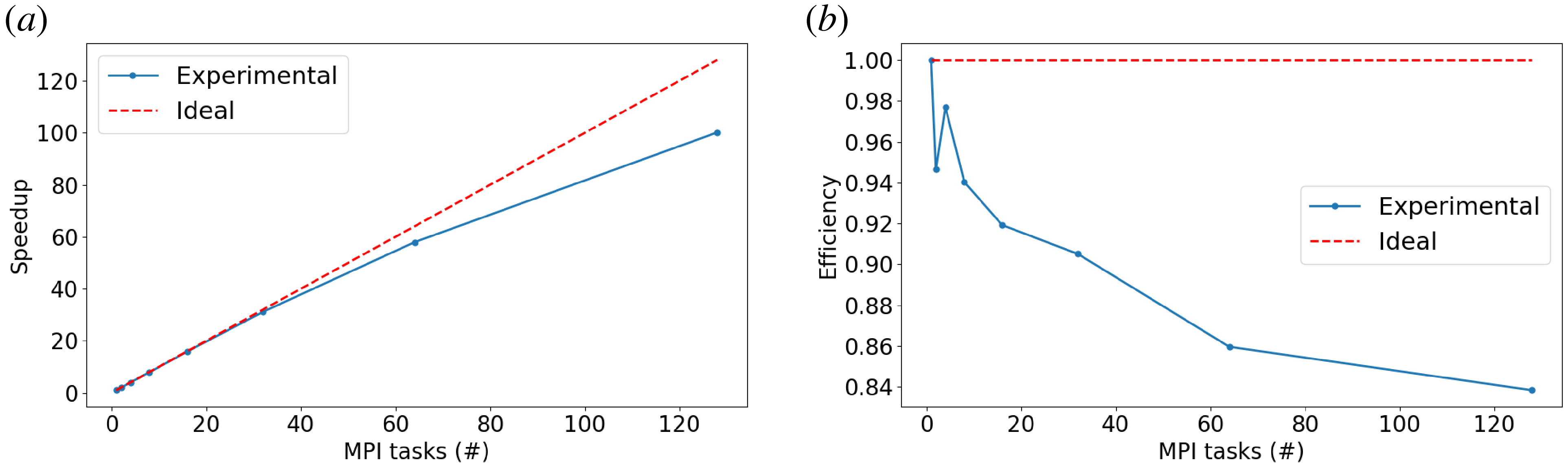

 Open access

