





Introduction
Climate change accelerates glacial melt and increases freshwater export from glaciers and ice sheets to the ocean, which can affect regional ocean circulation and potentially global thermohaline circulation (Oltmanns and others, Reference Oltmanns, Karstensen and Fischer2018; Rezvanbehbahani and others, Reference Rezvanbehbahani, Stearns, Keramati, Shankar and van der Veen2020). The solid component of this fresh water is exported as icebergs that calve from terminating marine glaciers and account for approximately 30–50% of the ice sheet’s mass loss to liquid fresh water (Moon and others, Reference Moon, Sutherland, Carroll, Felikson, Kehrl and Straneo2018). Since iceberg melt peaks later than other sources, quantifying iceberg volume and density is critical to understanding climate-driven discharge dynamics. Sudden increases in glacier flow, such as surges, can rapidly increase iceberg populations (e.g., Bailey and Marino, Reference Bailey and Marino2020; Singh and others, Reference Singh, Kumar and Kumar2023), amplifying freshwater release. At the same time, climate change has caused a dramatic decline in Arctic sea ice (IPCC, 2023), opening new shipping routes that significantly reduce travel distances (Christensen and others, Reference Christensen, Georgati and Arsanjani2019). This will increase the risk of icebergs-related hazards, such as ship collisions, highlighting the need for improved monitoring and predictive strategies for floating icebergs of all sizes. Consequently, tracking glacier ice discharge can potentially serve as an early warning system for elevated iceberg densities in adjacent fjord systems and coastal areas, particularly since sudden accelerations in glacier flow, such as short-term surges commonly observed in this region (Lovell and others, Reference Lovell2023), can lead to increased iceberg calving. This case study aims to quantitatively compare the total volume of detected icebergs based on remote sensing techniques with observations of glacier discharge.
Historically, iceberg information has relied on ship-based observations and aerial surveys, which are limited in spatial and temporal resolution (e.g., Lu and others, Reference Lu, Li, Shi and Huang2013). Advances in remote sensing have significantly improved monitoring capabilities, and several studies have explored automated detection methods. Current operational algorithms primarily use Synthetic Aperture Radar (SAR) imagery, as microwave signals penetrate polar atmospheres under adverse weather conditions. Icebergs appear bright in SAR images due to strong backscatter, allowing routine detection of those larger than the image resolution—typically 20–100 m for satellite-based SAR. Despite progress, challenges remain. Icebergs smaller than SAR resolution are inherently overestimated (e.g., Buus-Hinkler and others, Reference Buus-Hinkler, Qvistgaard and Krane2014; Šmejkalová and others, Reference Šmejkalová, Buus-Hinkler, Fleming, Gråbak, Power and Rasmussen2016; Karvonen and others, Reference Karvonen, Gegiuc, Niskanen, Montonen, Buus-Hinkler and Rinne2021), and other bright targets, such as ships or rough sea ice, can be misclassified as icebergs. Discrimination methods are being developed to segment ships from icebergs to address this (e.g., Heiselberg and others, Reference Heiselberg, Sørensen, Heiselberg and Andersen2022; Jafari and others, Reference Jafari, Karami, Taylor and Bobby2023). Monitoring in ice-covered waters is generally excluded for most coastal polar regions from October to May.
Cloud-free optical imagery is commonly used as a reference for validating SAR-based iceberg detection algorithms (e.g., Fenger-Nielsen, Reference Fenger-Nielsen2014; Soldal and others, Reference Soldal, Dierking, Korosov and Marino2019). Where high-resolution optical images have the potential to resolve icebergs of less than 15 m in length, depending on their resolution, they are hindered by cloud cover and darkness. Additionally, false detections by ships, failed detection in ice mélange (Podgórski and Petlicki, Reference Podgórski and Petlicki2020) and seasonal constraints due to the presence of sea ice remain a challenge. Here, we estimate iceberg size and volume using cloud-free, high-resolution (1.6 m) SPOT 6 and SPOT 7 optical images, applying a supervised classification approach, which is more robust than the simple threshold-based methods used in previous studies e.g.,
Sulak and others (Reference Sulak, Sutherland, Enderlin, Stearns and Hamilton2017). Podgórski and Petlicki (Reference Podgórski and Petlicki2020) utilized a more sophisticated object-based image analysis in a pro-glacial lagoon in Chile, which demonstrated high accuracy in the detection of icebergs of all sizes in the open lake, although many small icebergs (5–15 m $^2$) remained undetected.
The typical iceberg detection from satellite images (SAR and optical) provides information on iceberg features in either one or two dimensions, that is, length or sea-surface cross-sectional area, referred to herein as area. The third dimension, that is, the iceberg freeboards have been successfully measured using various satellite techniques, including Interferometric Synthetic Aperture Radar (InSAR)-derived Digital Elevation Models (DEMs) (Dammann and others, Reference Dammann2019), shadow length analysis from optical imagery (Guan and others, Reference Guan, Cheng, Liu, Li, Zhang and Yu2021; Suo and others, Reference Suo2024) and satellite altimeters, particularly in the interferometric mode, have been used to estimate iceberg freeboards in both hemispheres (e.g., Tournadre and others, Reference Tournadre, Whitmer and Girard-Ardhuin2008, Reference Tournadre, Bouhier, Boy and Dinardo2018; Braakmann-Folgmann and others, Reference Braakmann-Folgmann, Shepherd and Ridout2021, Reference Braakmann-Folgmann, Shepherd, Gerrish, Izzard and Ridout2022). Converting above-sea-surface characteristics to iceberg volume from satellite observations, particularly imagery, is challenging because these observations do not provide the information required for iceberg-specific conversions, which typically depend on iceberg height and shape (Diemand, Reference Diemand2001). In this study, we used a unique photogrammetric dataset from a field experiment to derive an area–volume relationship specific to this region.
Study area
Our case study is conducted in Upernavik Isfjord, Northwest Greenland (Fig. 1). The primary source of iceberg production is five main outlet glaciers with surface velocities exceeding 0.5 m d $^{-1}$ during the study period. Several other less productive glaciers also calve in the fjord. To quantify ice discharge from these glaciers, we use flux gates, that is, cross-sectional transects through which ice flux is estimated from velocity and thickness data. The flux gates from Mankoff and others (Reference Mankoff, Solgaard, Colgan, Ahlstrøm, Khan and Fausto2020) cover five (Fig. 1, blue lines) marine-terminating glaciers that calve into Upernavik Isfjord. The flux gate was placed as close to the glacier Calving Front Location (CFL) without compromising the thickness gate, which is associated with larger uncertainties near the CFL (Morlighem and others, Reference Morlighem2017).
Upernavik Isfjord is 60 km long from its eastern to its western boundary, that is, the length of the study area (Fig. 1, green outline). During winter, the fjord is covered by land-fast sea ice, also known as fjord ice. To limit the impact caused by the challenges related to the detection of icebergs in sea ice-covered waters, our study period is obtained during the open water season (see Appendix A). The outer fjord, corresponding to UP_1–UP_3 in Fig. 1, has steep-sided walls and a relatively flat bottom over 900 m deep (Vermassen and others (Reference Vermassen2019), their Fig. 1). Close to UP_4 there is a shallower area perpendicular to the fjord with water depths of about 650 m. Near the CFL close to the coast, in the branch south of UP_4, the water depths are relatively shallow (70–500 m), while the branch north of UP_4 remains deep ( $\sim$700 m) close to the CFL. The northern branches between UP_3 and UP_4 are shallow, with depths less than 200 m. Since icebergs in the Upernavik Isfjord are expected to have keel depths of less than 200 m, only areas with bathymetry shallower than 200 m are prone to iceberg grounding.
Study area in Upernavik Isfjord, Northwest Greenland. The background shows a SPOT mosaic (1.6 m resolution) visible in water areas, overlaid on land by a glacier surface-velocity map (white = 0 m d $^{-1}$, increasingly red with higher velocities). Black velocity vectors (greater than 0.5 m d
 $^{-1}$) are superimposed on the velocity field. The green polygon delineates the area used for iceberg quantification; four sites within this area (UP_1–UP_4) mark locations used for statistical analysis of sea ice presence (see Appendix A). In the bottom row, the green polygon is shown again (left) and subdivided into sections A–C corresponding to the inner, central and outer fjord, respectively. These sections also indicate the SPOT acquisition dates (all in the year 2020) covering each sub-area: A = 20 August, B = 18 July and C = 29 August. The subsequent panels illustrate the workflow from satellite data to iceberg metadata: zoomed SPOT imagery, the corresponding iceberg polygons derived from the binary iceberg–open water classification, and an example table of calculated iceberg properties. Iceberg metadata include the acquisition date/time, length, area and volume (the latter estimated using Eqn (2)).

Figure 1 Long description
The map of Upernavik Isfjord, Northwest Greenland, displays ice velocity with a gradient from white (0 m/day) to red (3.74 m/day). Black velocity vectors indicate speeds greater than 0.5 m/day. Flux gates are marked with blue lines. A green polygon outlines the region for iceberg quantification, subdivided into sections A, B and C, with SPOT acquisition dates: A on August 20, B on July 18 and C on August 29, 2020. The map includes zoomed sections showing iceberg polygons derived from binary classification. An inset map of Greenland highlights the study area. A table lists iceberg metadata, including acquisition date/time, length, area and volume. The map integrates satellite data to analyze iceberg properties and ice discharge from glaciers.
Data
We have two unique datasets: 1) Earth Observation data from 2020 including SPOT satellite images and measurements of ice-sheet solid ice discharge, and 2) field data from 2013 including a 3D photogrammetric dataset of 22 icebergs, as well as drift-derived vectors for 16 icebergs, obtained from TerraSAR-X. For the 2013 dataset, six of the icebergs are present in both datasets.
SPOT images
The SPOT 6 and SPOT 7 satellites, operated by Airbus Defence and Space (European Space Agency, n.d.), provide high-resolution optical imagery with a spatial resolution of 1.5 m (panchromatic) and 6 m (multispectral). Each satellite carries the New AstroSat optical Modular Instruments and captures data in five spectral bands: Panchromatic (0.45–0.75 µm), Blue (0.45–0.52 µm), Green (0.53–0.60 µm), Red (0.62–0.69 µm) and Near Infrared (0.76–0.89 µm). SPOT 6 remains operational, while SPOT 7 ceased operations in March 2023. SPOT 6 and SPOT 7 operated together or separately, with swath widths of 120 and 60 km, respectively. Their 26 day repeat orbits enable daily revisits at this latitude when both were active, and 1–3 days with a single satellite.
For this study, we used a mosaic of cloud-free SPOT 6 and SPOT 7 images prepared by the Danish Agency for Climate Data (KDS). The mosaic consists of ortho-rectified Digital Ortho Photos with a resolution of 1.6 m per pixel, generated using Airbus’ WorldDEM4ortho. The geometric accuracy is estimated to be 16 m (10 pixels) or better. The images of Upernavik Isfjord were collected during the 2020 open water season on six dates (18 July, 20 July, 20 August, 29 August, 9 September and 12 September). Although the mosaic spans 56 days, the analysis region used for the iceberg statistics (green polygon in Fig. 1) overlaps with only three of these dates (18 July, 20 August and 29 August).
3D photogrammetric iceberg data
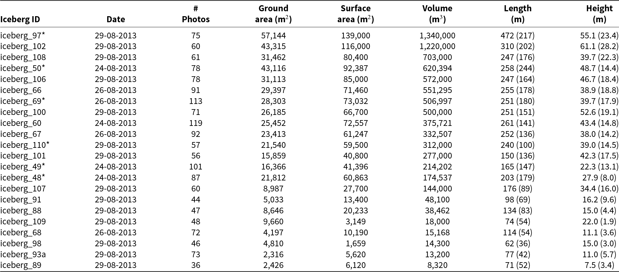
The unique collection of photo scans of 22 icebergs in Upernavik Isfjord was captured between 24 and 29 August 2013, during a field trip to Upernavik Isfjord. We used a Nikon D5000 camera with a fixed lens and captured photos while circumnavigating each iceberg in a research vessel. A minimum overlap of 60% was maintained between each picture. The photo scans of each iceberg contain a total of 36–119 photos, depending on the size of the iceberg. The position of each photo was recorded using a Global Navigation Satellite System (GNSS) receiver. Examples of photos from the photo scan dataset are provided in Fig. 2. The measured and derived characteristics of the icebergs, together with examples of the derived iceberg topography corresponding to those presented in Fig. 2, are provided in Appendix B.
Photo examples from the iceberg photo scan dataset. Left: Iceberg 60 (24 August 2013) length 216 m, maximum sail height 43 m, mean freeboard height 5.2 m, area 25 452 m $^2$ and volume 3 595 650 m
 $^3$. Right: Iceberg 68 (26 August 2013) length 114 m, maximum sail height 11 m, mean freeboard height 1.5 m, area 4197 m
 $^2$ and volume 145 159 m
 $^3$.

TerraSAR-X
The German TerraSAR-X satellite mission operates in the X-band (9.6 GHz) and is equipped with a phased array SAR antenna that acquires high-resolution radar images regardless of weather and illumination. It supports single, dual and quad polarization and offers three main imaging modes: SpotLight (up to 1 m resolution), StripMap (up to 3 m) and ScanSAR (up to 16 m) (Roth and others, Reference Roth, Eineder and Schättler2014). TerraSAR-X uses an adjustable-angle radar sensor to observe any location on Earth within 1–3 days, while maintaining high radiometric resolution at varying spatial resolutions.
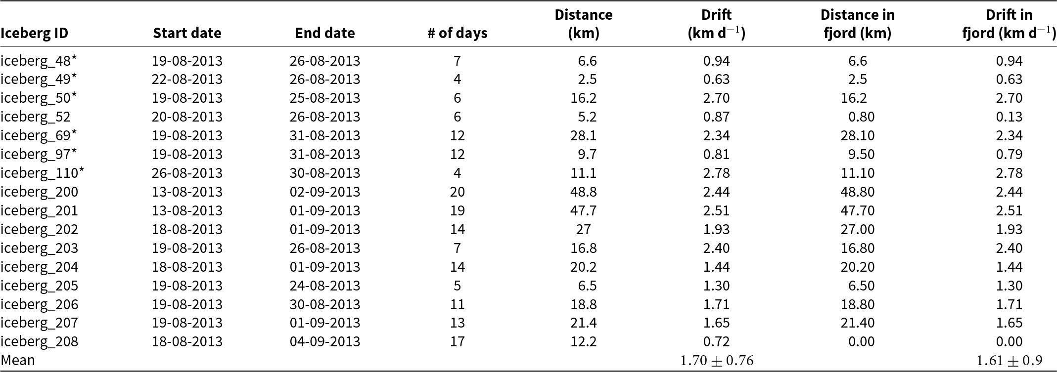
Here, we used a series of daily TerraSAR-X satellite images acquired between 13 August and 4 September 2013 to estimate the iceberg drift speeds for 16 selected icebergs (presented in Appendix C), where six of the icebergs (with iceberg IDs 48, 49, 50, 69, 97 and 110) are the same as those included in the 3D iceberg photo study.
Ice-sheet solid ice discharge
We used estimated Greenland ice sheet solid ice discharge from Mankoff and others (Reference Mankoff, Solgaard, Colgan, Ahlstrøm, Khan and Fausto2020), produced as part of the Programme for Monitoring of the Greenland Ice Sheet (PROMICE). The dataset provides fluxes at predefined gates located near the grounding line or glacier front for all major marine-terminating outlet glaciers. Discharge is calculated by combining satellite-derived surface velocities with estimates of ice thickness from various sources. For this study, we used the combined discharge from flux gates 133–137, which covers the region of interest in our analysis (Fig. 1). The complete dataset is available from the PROMICE data portal (Mankoff and Larsen, Reference Mankoff and Larsen2020).
Method
In this study, we classify and detect iceberg sizes (length and area) from the SPOT mosaic and convert area to volume using photogrammetric data from a field experiment on representative icebergs in Upernavik Isfjord. This enables us to derive an area–volume relationship specific to the region. Using this relationship, we produce size and volume distributions, as well as an estimate of the total iceberg volume in the fjord, by treating the SPOT mosaic as a snapshot of the iceberg distribution and assuming conservation of total iceberg volume during the acquisition period. Additionally, we estimate the average daily glacier discharge from Mankoff and Larsen (Reference Mankoff and Larsen2020) of the five most productive outlet glaciers over the period covered by the SPOT mosaic. To compare with the total satellite-derived iceberg volume, we integrate the average daily glacier discharge over the expected iceberg residence time in Upernavik Isfjord, using an average drift speed extracted from successive TerraSAR-X images. Finally, we compare the SPOT-derived iceberg volume with the integrated glacier discharge and discuss the associated uncertainties and missing contributions needed to close the ice volume budget.
Automated detection of icebergs from SPOT images
We applied a supervised classification method to the SPOT images using the Minimum Distance algorithm. For this procedure, we utilized the Semi-Automatic Classification Plugin developed by Congedo (Reference Congedo2021) within the QGIS environment. This plugin facilitates the supervised classification and provides tools for the downloading, pre-processing and post-processing of remote sensing images.
The training dataset was developed by manually identifying three classes: 1) ice, 2) open water and 3) land (or rock). For this purpose, a representative image that exhibits high variability was selected, including different rock types, water depths and ice conditions (e.g., icebergs, glaciers and mélange). Within this image, Regions of Interest (ROIs), that is, manually delineated and labeled training polygons, were created for each class. These ROIs provide samples of the spectral reflectance associated with each surface type and form the basis for training the classifier.
To ensure a robust representation of the spectral variability, approximately 40 small polygons of similar size were uniformly distributed throughout the scene. The number and placement of ROIs were determined through iterative testing to balance classification accuracy, computational efficiency and the large volume of images to be processed. The spectral information extracted from these ROIs was then applied to classify the remaining SPOT images.
Although imagery is generally of high quality, variations in atmospheric conditions, solar illumination and sensor characteristics (e.g., between SPOT 6 and SPOT 7) can introduce inconsistencies in the classification. To address this, preprocessing steps were applied, including normalization and feature extraction using Principal Component Analysis.
The classification was performed using a supervised machine learning approach based on a Support Vector Machine (SVM), selected for its robustness and efficiency in handling large datasets. The SVM was trained using the labeled ROI dataset, with model parameters optimized through a grid search procedure. The performance of the classification was evaluated by comparison with manual operator classification, demonstrating a substantial reduction in processing time while maintaining a high level of accuracy. The final training dataset was carefully evaluated to ensure that all classes were adequately represented and that the full range of spectral variability was captured.
The classification output is stored in a raster file, where each pixel is assigned a value corresponding to one of the three classes. For further analysis, the raster was processed using the Python GDAL and OGR modules to convert contiguous pixels classified as ice into vector polygons. Each polygon representing an iceberg was then attributed with its geometric properties (i.e., area and length), where iceberg lengths were calculated as the maximum distance between two vertices of each iceberg polygon. An example of the workflow based on a subset of the SPOT imagery to iceberg metadata is shown in Fig. 1.
Iceberg area–volume conversion
The relationship between iceberg area (A) as derived from the SPOT images and (above- and below-water) volume (V) is established from the 3D photo scan study. To estimate freeboard (above-water) volume ( $V_{free}$) and associated area of each photoscanned iceberg, we used Agisoft Photoscan and QGIS, following the process diagram outlined in Fig. 3. The procedure is to a large degree automated but requires the following manual steps: 1) The dense point cloud includes points not only from the iceberg surface but also from other neighboring icebergs, ice mélange, clouds and visible land. These extraneous points are manually deleted, leaving only the points of the relevant iceberg surface. 2) The generated mesh, based on the dense point cloud, requires editing. This is necessary because the dense point cloud includes areas without data points. In such cases, Agisoft extrapolates parts of the surface that must be removed. The absence of data points is due to parts of the iceberg shape being below the water surface, and, in many cases, parts of the iceberg are not visible in the photos.
Process diagram for estimating iceberg freeboard volume and associated area, with the use of Agisoft Photoscan and QGIS. Manual steps are indicated by green boxes.

Once  $V_{free}$ has been estimated, the total volume of each iceberg is given using the assumption of hydrostatic equilibrium;
 \begin{equation}
V = \frac{V_{free}}{1-\rho_{ice}/\rho_{w}},
\end{equation}
where  $\rho_{ice}$=917 kg m
 $^{-3}$ and
 $\rho_{w}$=1024 kg m
 $^{-3}$ are the densities of ice and seawater, respectively. Finally, the relationship between
 $A$ and
 $V$ is established by the best fit of the general power law, as suggested by Sulak and others (Reference Sulak, Sutherland, Enderlin, Stearns and Hamilton2017).
Results
The best-fitting power law between  $A$ and
 $V$, based on our iceberg photo study in Upernavik Isfjord, is presented in Fig. 4 and is expressed as;
 \begin{equation}
V=0.2 \times A^{1.64},
\end{equation}
with a correlation of 0.91. Sulak and others (Reference Sulak, Sutherland, Enderlin, Stearns and Hamilton2017) used a similar approach; however, instead of deriving the area–volume relationship based on photogrammetric field data, they generated iceberg DEMs from high-resolution ( $\sim$0.5 m) stereo imagery from Worldview 1–3 satellites. Their results are based on observations of 712 icebergs in the Sermilik Fjord in Southeast Greenland. To compare our results with theirs, we added their best-fit power laws, including their 95% confidence intervals, to Fig. 4.
Iceberg area–volume (above and below the ocean surface) best-fit power–law relationship (black dotted line) based on our 3D photoscanned icebergs (black triangles), together with results presented by Sulak and others (Reference Sulak, Sutherland, Enderlin, Stearns and Hamilton2017). A full-scale plot of the extrapolation beyond the calibration domain is provided in Appendix D, Fig. D1.

Figure 4 Long description
Equastions of the best-fit power-laws of Sulak and others (2017) and our approach with corresponding total volumes are inserted in the upper part of the figure. Sulak and others (2017) based on 712 observations with upper and lower 95% confidence intervals (V=8.6A1.33, V=6.0A1.30, V=3.4A1.28), correspoinds to total volumes of 9.3 km3, 4.9 km3 and 1.9 km3, respectively. Our best-fit power-law, based on 22 observations, V=0.2A1.64 correspond to a total iceberg volume in Upernavik Isfjord of 4.7 km3. A graph with a horizontal axis labeled Iceberg Sea Surface Cross Sectional Area (m2) and a vertical axis labeled Iceberg Volume (m3). The horizontal axis shows labeled ticks ranging between 0 and 60,000. The vertical axis shows labeled ticks ranging between 0 and 300,000. The three solid curves rise from near the origin and are the best-fit power-law (green) Sulak and others (2017) approach with 95% confidence intervals (upper limit red and lower limit blue). The dotted curve rises from near the origin and is associated with our best-fit power-law. A set of triangular markers is plotted along the lower left to mid right portion of the graph, which represent our 22 observed icebergs.
The lengths of the 22 icebergs in the 3D photo scan study range from a minimum of 62 m (Appendix B, iceberg_98) to a maximum of 472 m (Appendix B, iceberg_97). In the following, we use the term ‘calibration domain’ for icebergs within this range. Thus, for icebergs shorter than 62 m and longer than 472 m, the relationship between  $A$ and
 $V$ has been extrapolated (Appendix D, Fig. D1). As seen, our best-fit power law is within the upper bound of the 95% confidence interval for icebergs with an area less than about 150 000 m
 $^2$. Measurement uncertainties for the 3D photogrammetric data are estimated from a repeatability analysis (presented in Appendix B), yielding uncertainties of ∼ 5% for volume and ∼ 6% for ground area. These values are representative only within the calibration domain.
Iceberg size and volume distribution from SPOT imagery
In our study, we detected and classified a total of 343 769 icebergs by size in Upernavik Isfjord using SPOT images. The smallest detected growlers were close to the resolution limit of the SPOT images, that is, approximately 1.6 m in length, with an associated area of 2.6 m $^2$. The largest identified icebergs (i.e., one that is not mélange) were found to be more than 1000 m in length. In total, 83 959 icebergs were classified as having a length of
 $\ge$15 m, with only 1584 of these classified as large or very large icebergs (
 $ \gt 120~\mathrm{m}$).
The iceberg concentration in Upernavik Isfjord, provided as counts per km $^2$ for icebergs
 $\ge$15 m, is presented in Fig. 5a, with icebergs
 $ \gt 120~\mathrm{m}$ marked in black. The associated iceberg concentration, including bergy bits and growlers (
 $ \lt 15~\mathrm{m}$), is presented in Fig. 5c. There is a very high concentration of icebergs in the inner fjord, exceeding 3000 counts per km
 $^2$ near the most productive outlet glaciers, particularly when bergy bits and growlers are included, as expected. The central part has a lower iceberg density, where individual icebergs can be seen. In contrast, there is a lower density in the westernmost area. This pattern reveals that most of the growlers and bergy bits deteriorate before reaching the open sea. The area immediately adjacent to the CFL is not included in this study (Fig. 5, white patch), as it is packed with icebergs and ice mélange throughout the year, making classification difficult (Andresen and others, Reference Andresen, Kjeldsen, Harden, Nørgaard-Pedersen and Kjær2014).
Iceberg concentration (count per 1 km $^2$) in Upernavik Isfjord within the area of interest, see Fig. 1, where also the full glacier outlets and flux gate locations are shown. The black polygons are icebergs (sea-surface cross-sectional areas as seen in the SPOT imagery) with a horizontal length
 $ \gt 120~\mathrm{m}$. These icebergs make up about 87% of the glacial ice volume in the fjord. (a) shows the concentration of icebergs, that is, glacial ice objects
 $\geq$ 15 m in length. (b) is a zoomed subset of (a). The concentrations displayed in (c) also include growlers and bergy bits, that is, glacial ice objects
 $ \lt 15~\mathrm{m}$ in length.

Figure 5 Long description
A) The map shows iceberg concentration in Upernavik Isfjord, Greenland, with values ranging from 0 to over 3000 icebergs per km2. High concentrations, exceeding 3000 icebergs per km2, are found in the inner fjord, particularly near outlet glaciers. B) This is a zoomed-in section of A, highlighting individual icebergs as black polygons. C) The map includes smaller icebergs, growlers and bergy bits, showing a similar pattern with high concentrations in the inner fjord and lower densities towards the westernmost area. The legend indicates iceberg density categories from 0 to 3000 icebergs per km2, with specific color codes for each range.
We present the iceberg size distribution in Fig. 6, classified according to length as defined by the sea ice nomenclature in the World Meteorological Organization (2014), with additional classes above 200 m. Based on our area–volume relationship (Eqn (2)), we estimate the volume of each iceberg, as well as the total volume of all detected icebergs in Upernavik Isfjord. The total volume is found to be 4.7 km $^3$. We do not report a combined uncertainty on total volume because measurement uncertainties are only constrained within the calibration domain, no explicit uncertainty is available for the SPOT-derived areas, and the limited calibration sample size (22 icebergs) precludes robust statistical uncertainty propagation. For comparison, applying the best-fit power law from Sulak and others (Reference Sulak, Sutherland, Enderlin, Stearns and Hamilton2017) to our SPOT-derived areas yields a total iceberg volume of 4.9 km
 $^3$, with a 95% confidence interval ranging from 1.9 to 9.3 km
 $^3$. Although Sulak and others (Reference Sulak, Sutherland, Enderlin, Stearns and Hamilton2017) is based on observations from a different fjord system in Greenland, this result provides some confidence in our estimate. Regional differences may also explain the differences in estimates of total iceberg volume.
Iceberg size and volume distribution in Upernavik Isfjord from SPOT images. Number of detected icebergs from SPOT images and 3D photo scan field experiment (shown in parenthesis) is presented above each column (blue) for each length category. Volumes are shown as percentages of the total volume of all detected icebergs from SPOT. Iceberg length categories ( $x$-axis): For each category, numbers in parentheses give the mean sea-surface cross-sectional area of the icebergs, and numbers in brackets give the standard deviation of that mean.

Figure 6 Long description
The vertical axis on the left is labeled Number of icebergs, ranging from 0 to 300000. The vertical axis on the right is labeled Percentage of total volume, ranging from 0 to 25. The horizontal axis shows iceberg length categories with rotated labels. Bars and values shown above the bars: 1) 0 to 50: Number of icebergs 259,810 with (0) in parentheses; Percentage of total volume 0.4%. 2) 50 to 100: Number of icebergs 77,419 with (0) in parentheses; Percentage of total volume 4.3%. 3) 100 to 150: Number of icebergs 4,956 with (0) in parentheses; Percentage of total volume 8.3%. 4) 150 to 200: Number of icebergs 1,098 with (0) in parentheses; Percentage of total volume 12.9%. 5) 200 to 250: Number of icebergs 884 with (11) in parentheses; Percentage of total volume 24.0%. 6) 250 to 300: Number of icebergs 72 with (1) in parentheses; Percentage of total volume 20.5%. 7) 300 to 400: Number of icebergs 27 with (0) in parentheses; Percentage of total volume 22.8%. 8) 400 to 500: Number of icebergs 3 with (0) in parentheses; Percentage of total volume 6.8%. The number in paranthesis denotes the number of icebergs in that specific size category from our observed iceberg in the field study.
We present the percentage contribution of each iceberg class to the total volume in Fig. 6. Applying Eqn (2) to the icebergs detected from SPOT imagery involves extrapolation beyond the calibration domain, especially for the largest size classes. To assess the implications, we examine mean areas, their variability, population counts and relative contributions to the total estimated volume across length categories.
(1) Bergy bits and growlers (
 $ \lt 15~\mathrm{m}$): This smallest category contains the majority of the population (259 810 icebergs, ∼ 76% of the dataset). Their mean cross-sectional area is very small (∼ 35 m
$^2$) with low variability (∼ 18 m
$^2$). Despite their numerical dominance, they contribute less than 0.5% of the estimated total volume. Thus, while statistically important to represent the full size spectrum, they are volumetrically negligible and do not significantly affect overall volume estimates.
(2) Small to large icebergs (15–200 m): This group (∼ 78 000 icebergs) shows progressively larger mean areas (259–7998 m
$^2$) with moderate variability (253–3549 m
$^2$). They contribute ∼ 25% of the total volume. These sizes are well within the calibration domain, and uncertainties are therefore modest relative to their contribution.(3) Very large icebergs (200–500 m): Rare in number (456 icebergs, ∼ 0.1% of the dataset), but with substantial mean areas (22 028–56 377 m
$^2$) and high variability (10 451–23 469 m
$^2$). They contribute ∼ 45% of the total volume. Although the upper end of this range approaches the calibration limit, estimates remain broadly supported by measured icebergs.(4) Huge icebergs (
$ \gt 500~\mathrm{m}$): Only 30 icebergs exceeded 500 m in length, including just three larger than 1000 m (
$ \lt 0.01\%$ of the population). Their mean areas are huge (104 440 –
$ \gt 209\,925\,\mathrm{m}^2$) with high variability (standard deviations up to ∼ 63 000 m
$^2$). Yet they account for ∼ 30% of the estimated total volume. For this group, the function is entirely extrapolated, and their rarity combined with disproportionate volume contribution means that they dominate the overall uncertainty.


In summary, the dataset is strongly skewed: the majority of icebergs are bergy bits and growlers, but these contribute very little to the volume budget. About 70% of the estimated volume comes from icebergs smaller than 500 m, where the area–to-volume relationship is applied within or close to the calibration domain, ensuring relatively robust estimates. The remaining ∼ 30% of the total volume arises from very large icebergs ( $ \gt 500~\mathrm{m}$), which are extremely rare but dominate the uncertainty because their volumes are estimated by extrapolation beyond the measured range (e.g., the largest detected iceberg contains 5.0% of the total volume).
Glacier solid ice discharge
The average glacier discharge and its associated uncertainties for the selected time periods, extracted from Mankoff and Larsen (Reference Mankoff and Larsen2020), together with the corresponding temporal discharge (i.e., total discharge over the given time period), are presented in Table 1. Based on these values, we estimate the daily discharge and its associated uncertainties assuming an ice density of 917 kg m $^{-3}$. According to Mankoff and others (Reference Mankoff, Solgaard, Colgan, Ahlstrøm, Khan and Fausto2020), the measurement uncertainties are about 10% of the discharge. The dominant contribution to this uncertainty arises from ice thickness, in particular the ice bed location, whereas uncertainties in ice velocity are comparatively small.
Average discharge and error from Mankoff and Larsen (Reference Mankoff and Larsen2020), temporal discharge (total over the time period), and estimated daily glacier discharge into Upernavik Isfjord with related uncertainty.

Table 1 Long description
The table lists weekly glacier discharge into Upernavik Isfjord from 1 July to 1 September 2020, giving average discharge and its error, total discharge over each week, and estimated daily discharge with uncertainty. Average discharge ranges from 45.60 to 48.53 Gt a-1, with errors from 4.31 to 4.56 Gt a-1. The highest average discharge occurs 22 to 28 July at 48.53 Gt a-1,, and the lowest occurs 26 August to 1 September at 45.60 Gt a-1,. Weekly total discharge is tightly clustered between 0.87 and 0.93 Gt, peaking in late July and late July to early August. Daily discharge varies from 0.136 to 0.145 km3 d-1, with uncertainty about 0.013 to 0.014 km3 d-1. Overall, discharge rises slightly from early July into late July, then gradually declines through late August. A mean row summarizes the period at 47.44 Gt a-1, average discharge, 0.91 Gt weekly total, and 0.142 km3 d-1 daily discharge, with mean uncertainty 0.013 km3 d-1.
The average daily glacier discharge for 1 July to 1 September 2020 is estimated to be  $0.142\pm0.013$ km
 $^3$ d
 $^{-1}$. Maximum ice discharge (
 $0.145\pm0.014$ km
 $^3$ d
 $^{-1}$) is observed at the end of July, while minimum ice discharge (
 $0.136\pm0.013$ km
 $^3$ d
 $^{-1}$) is observed at the end of August. The average net drift of icebergs out of the fjord system is
 $1.6\pm0.9$ km d
 $^{-1}$ (Appendix C, Table C1), where the uncertainty denotes the standard deviation. Given a distance of 60 km between the inner and outer fjord in our study area, the mean residence time of an iceberg is estimated to be 37.5 days, ranging from 24.0 to 85.7 days based on drift uncertainty. Thus, the total glacier discharge is estimated to be
 $5.3\pm0.5$ km
 $^3$, integrated over the 37.5 days it takes for icebergs to travel from the inner fjord to the open ocean, with a corresponding range of
 $3.4\pm0.3$ to
 $12.2\pm1.1$ km
 $^3$.
Discussion
Our SPOT-derived total iceberg volume of 4.7 km $^3$ represents 88.7% of total glacier discharge and lies well within the corresponding discharge range of 3.4–12.2 km
 $^3$. Uncertainties in the area–volume relationship, based on the 95% confidence intervals reported by Sulak and others (Reference Sulak, Sutherland, Enderlin, Stearns and Hamilton2017), are substantial but comparable in magnitude to the discharge range associated with residence time. To our knowledge, this is the first study to link observations of glacier calving with a contemporaneous snapshot of iceberg volume in a fjord system, highlighting the potential for integrating multiple satellite datasets and methodologies. However, it is important to acknowledge the uncertainties and assumptions inherent in our approach and to assess how they affect our results. Where measurement uncertainties are relatively small (∼ 5% for icebergs within the calibration domain and ∼ 10% for glacier discharge; Mankoff and others, Reference Mankoff, Solgaard, Colgan, Ahlstrøm, Khan and Fausto2020), the dominant uncertainties arise from methodological assumptions, which are discussed in more detail below.
Geometric scaling and limits of extrapolation
A substantial portion of the fjord’s total volume (∼ 30%) is concentrated in a small population of large icebergs ( $ \gt 500~\mathrm{m}$). While our internal 3D photogrammetric calibration is based on icebergs up to 472 m in size, applying the power–law relationship (Eqn (2)) to larger classes represents the most viable methodological approach given current data constraints. Regional studies (e.g., Sulak and others, Reference Sulak, Sutherland, Enderlin, Stearns and Hamilton2017) support the general applicability of area–volume relationships; however, extending these relationships beyond the calibration domain assumes geometric scale invariance, which is difficult to verify. Consequently, this extrapolation represents a notable source of uncertainty, as larger icebergs may deviate from the morphology of smaller fragments due to differences in calving dynamics or structural evolution. Nonetheless, in the absence of direct 3D observations of the largest icebergs, this approach provides the most robust available framework for estimating regional iceberg volume.
The dominance of the largest icebergs in the total volume implies that any biases associated with this extrapolation can disproportionately affect the overall estimate. In addition, potentially double-counted or undetected icebergs would further influence the derived totals.
As the SPOT mosaic (Fig. 1) is considered a composite representation of the iceberg population within the study area, it does not correspond to a true instantaneous snapshot due to the movement of the icebergs between acquisitions. The average residence time (37.5 days) in Upernavik Isfjord implies that some icebergs could, in principle, be captured more than once. Nevertheless, the predominantly outward transport of icebergs (Appendix C) strongly limits this possibility. The 33 day separation between the 18 July and 20 August scenes exceeds typical residence times for this region, and the 29 August coverage of the outer fjord occurs 42 days after the acquisition of the adjacent central fjord. In combination with the efficient removal of icebergs by the northward boundary current in Baffin Bay, repeated detection across the composite is unlikely. Although short-term reversals due to tidal currents and temporary grounding cannot be excluded, no clear cases were identified in the images. We therefore conclude that the probability of double-counting is small and that the SPOT mosaic provides a robust representation of the fjord-wide iceberg population despite the inherent limitations of temporal compositing.
Ice mélange and high concentration areas
Estimating iceberg volume using SPOT imagery presents significant challenges in regions with high iceberg concentration and in the presence of ice mélange ( $ \gt 1000$ icebergs per km
 $^{-2}$ in Fig. 5c). In such conditions, distinguishing individual icebergs from the surrounding mélange is challenging (as also noted by Sulak and others (Reference Sulak, Sutherland, Enderlin, Stearns and Hamilton2017)) or, in our case near the CFL, not feasible. While the mélange itself contributes little to the total volume, undetected icebergs within it may lead to an underestimation of the total volume, affecting the robustness of our results.
The leverage effect of density assumption
Absolute volume estimates remain highly sensitive to the assumed ice density ( $\rho_{ice}$). We adopt a standard value of 917 kg m
 $^{-3}$. For icebergs, this corresponds to a volume conversion factor of 9.57 (Eqn (2)). In particular, the density of calved ice can be locally modified by subglacial debris entrained during basal flow. Deep ice core records from Greenland, such as the GISP2 and Byrd cores (Gow and Meese, Reference Gow and Meese1996) and the NEEM basal sequence (Goossens and others, Reference Goossens, Sapart, Dahl-Jensen, Popp, El Amri and Tison2016), show that the lowermost meters of fast-flowing ice sheets can contain highly stratified layers with sediment mass concentrations of 12–15%.
To illustrate the sensitivity, we consider a simple scenario. Assuming a representative silicate sediment density ( $\rho_{sediment}$) of ∼ 2600 kg m
 $^{-3}$, a volumetric debris fraction of 1.4% would increase the bulk density to approximately 940 kg m
 $^{-3}$. If such material is preserved within an iceberg keel, the corresponding conversion factor would increase to 12.19. We emphasize that this value represents a theoretical upper bound for a local sensitivity test rather than a representative average for the fjord-wide iceberg population. Nevertheless, this example demonstrates that small, unobserved variations in debris content can lead to changes of up to 27% in estimated volume for subsets of icebergs. This represents a physical uncertainty that cannot be constrained from 2D surface observations alone.
While the adopted density is consistent with values used for glacier discharge estimates at flux gates (Mankoff and others, Reference Mankoff, Solgaard, Colgan, Ahlstrøm, Khan and Fausto2020), it is important to note that other processes can act in the opposite direction. For example, extensive crevassing can reduce the effective bulk density, leading to larger inferred glacier discharge volumes. Together, these competing effects highlight the sensitivity of volume estimates to poorly constrained density variations.
Temporal variance and the glacier discharge budget
In our study, iceberg residence times represent a major source of uncertainty in the estimated total glacier discharge, ranging between 3.4 and 12.2 km $^3$. The estimated residence times (24–86 days) are comparable to those reported by Sutherland and others (Reference Sutherland, Roth, Hamilton, Mernild, Stearns and Straneo2014), who found values between 8 and 94 days in Sermilik Fjord, East Greenland. This high variability directly influences the derived discharge.
Extended residence times are most likely associated with the grounding of large icebergs. However, only icebergs with drafts exceeding 200 m are likely to be grounded in Upernavik Isfjord, as areas shallower than 200 m are limited. Icebergs in this region are generally expected to have drafts less than 200 m (Andresen and others, Reference Andresen, Kjeldsen, Harden, Nørgaard-Pedersen and Kjær2014), suggesting that grounding events are relatively rare. In regions covered by ice mélange, that is, near the CFL, this introduces a potential conflict with one of the key assumptions of our study. If calving rates are linked to the instantaneous presence of icebergs in the fjord, then poorly constrained residence times within the mélange become a critical factor.
Ice discharge from glaciers outside the defined flux gates and region of interest may provide an additional source of uncertainty. For example, the glacier located north of the study area near UP $_{1}$ (Fig. 1) appears highly productive, although its contribution depends on local current dynamics. Glaciers located south of the study area are likely less productive, but may still contribute to icebergs. Any such external input would increase the glacier discharge.
Melt, accumulation and deterioration
In this study, we do not account for the deterioration of icebergs due to processes such as subsurface melt, solar radiation, buoyant convection, wave erosion and calving. Kubat and others (Reference Kubat, Sayed, Savage, Carrieres and Crocker2007) provide formulations to account for these processes, except subsurface melt, which could be incorporated to quantify their impact. Similarly, Moon and others (Reference Moon, Sutherland, Carroll, Felikson, Kehrl and Straneo2018) developed an iceberg melt model for the Helheim-Sermilik glacier-fjord system, showing that 68–78% of iceberg melt occurs below 20 m depth, with 40–100% of this melt remaining at depth depending on season.
If these processes contribute significantly to volume loss, the total volume would be underestimated relative to glacier discharge, which is consistent with our findings. This represents an additional source of uncertainty that cannot be constrained with surface observations alone.
Additional contributions may arise from melt and accumulation processes between the flux gate and the glacier terminus, as well as from the assumption that all ice passing through the flux gate exits the fjord as solid ice. However, these effects are likely minor compared to uncertainties associated with iceberg residence time.
Conclusion
In this study, we used a mosaic of high-resolution SPOT 6 and SPOT 7 images (1.6 m) to derive iceberg size distributions and estimate total iceberg volume in Upernavik Isfjord during the 2020 open water season. A total of 343 769 icebergs were detected. Volume estimates were obtained using an area–volume relationship constrained by regional 3D photogrammetric observations, allowing the conversion of satellite-derived cross-sectional surface area to iceberg volume.
Our results show a highly biased size distribution, where growlers and bergy bits represent  $\sim$76% of the population and contribute less than 0.5% of the total volume (4.7 km
 $^3$). In contrast, a very small fraction (
 $ \lt 0.01\%$) of large icebergs (
 $ \gt 500~\mathrm{m}$) contributes nearly a third of the total volume. As volume estimates for these large icebergs rely on extrapolation beyond the calibration domain, the total volume budget is highly sensitive to scaling assumptions. Targeted field observations of the largest icebergs would, therefore, substantially reduce uncertainties in future studies.
By integrating the estimated iceberg residence times, we derive a glacier discharge of  $5.3\pm0.5$ km
 $^3$, which varies between 3.4 and 12.2 km
 $^3$ when accounting for residence time variability. The SPOT-derived iceberg volume corresponds to 88.7% of this discharge, demonstrating general consistency between independent estimates. The dominant uncertainties arise from residence time variability, extrapolation of the area–volume relationship beyond the calibration domain and assumptions regarding iceberg density.
Future work will benefit from combining high-resolution optical observations with frequent SAR-based monitoring, such as Sentinel-1 data. Although SAR imagery has coarser spatial resolution, its all-weather capability and high temporal coverage allow for continuous monitoring of iceberg distribution and dynamics. Integrating these approaches offers great potential to improve estimates of iceberg volume, residence time and grounding processes across Greenland fjord systems.
Acknowledgements
This study was carried out in collaboration between the Danish Meteorological Institute (DMI) and the Technical University of Denmark (DTU). It was funded by the Danish State through the National Centre for Climate Research and by the European Union’s Horizon Europe research and innovation program under the Acciberg project (grant agreement No. 101081568). The authors thank the Danish Agency for Climate Data (Klimadatastyrelsen) for providing the SPOT images and the Geological Survey of Denmark and Greenland (GEUS) for glacier discharge data from the Programme for Monitoring of the Greenland Ice Sheet (PROMICE). We acknowledge the use of AI-based language tools (Copilot and ChatGPT) to assist in the verification of the manuscript for consistency and clarity. These tools were used to support language refinement without altering scientific content. Finally, we express our sincere appreciation to the editor and reviewers for their thoughtful and constructive evaluations. Their insightful comments and suggestions have been invaluable in improving the clarity and overall quality of the manuscript.
Appendix A. Sea ice concentration
Seasonal variations in sea ice concentration at four locations in Upernavik Isfjord (UP_1–UP_4; see Fig. 1). Sea ice concentration is expressed on a scale from 0 to 10, where 10 corresponds to 100% concentration (i.e., increments of 10%). The color coding is as follows:
– 0 (open water): blue
– 1–3 (low concentration): green
– 4–6 (medium concentration): yellow
– 7–8 (moderate–high concentration): orange
– 9–10 (high concentration): red
Figure A1.Seasonal variations of the sea ice coverage (provided as concentration) at four different locations in the Upernavik Isfjord as marked by UP_1 to UP_4 in Fig. 1.
Figure A1 Long description
The heatmaps display seasonal variations of sea ice coverage at four locations, UP 1 to UP 4, in Upernavik Isfjord. Each heatmap has rows labeled with weeks and dates from April 23 to December 24 and columns labeled with years from 2000 to 2021. The numerical values within the cells represent sea ice concentration percentages. A gradient from lower to higher values is indicated, with specific colors representing different concentration levels. Notable patterns include higher concentrations in earlier years and a tendency towards lower concentrations in recent years, particularly in the inner fjord (UP 4) compared to the outer fjord (UP 1). The heatmaps highlight interannual variability and a general trend towards a shorter open-water season in the inner fjord.

Based on ice charts from the Greenland Ice Service at the Danish Meteorological Institute (DMI), weekly sea ice concentration was estimated for the period 23 April to 24 December at the four locations UP_1–UP_4 in Upernavik Isfjord, as defined in Fig. 1, for the years 2000–21. These are shown in Fig. A1, where zero concentration (blue) marks the open-water season. There is substantial interannual variability, as well as a tendency towards a shorter open-water season in the inner fjord (UP_4) compared with the outer fjord (UP_1).
In 2020, the open-water season at UP_1 lasted from 21 May to 8 October, with only one brief low-concentration event (10%) during the week of 30 July. In the inner fjord (UP_4), fast ice persisted until the week of 28 May 2020, corresponding to high sea ice concentration ( $ \gt 70\%$). This was followed by the open-water season until the week of 28 September, with only occasional low-concentration events (
 $ \lt 30\%$), likely associated with iceberg break-up. Based on these observations, Upernavik Isfjord can be considered effectively ice-free from June to September 2020.
Appendix B. 3D photoscanned icebergs
The measured and derived characteristics of the icebergs from the photo study are provided in Table B1, together with examples of derived iceberg topography in Fig. B1.
Examples of the derived iceberg topography from the 3D photogrammetric dataset presented in Fig. 2. (a) Iceberg 60 (24 August 2013) with length 216 m, maximum sail height 43 m, mean freeboard height 14.8 m, area 25 452 m $^2$ and volume 3 595 650 m
 $^3$. (b) Iceberg 68 (26 August 2013) with length 114 m, maximum sail height 11 m, mean freeboard height 3.6 m, area 4197 m
 $^2$ and volume 145 159 m
 $^3$.

Measured and derived characteristics of icebergs from the 3D photo scan field experiment. Ground area is equal to the iceberg sea-surface cross-sectional area in Fig. 4. Volume refers to the above-sea-surface volume. Length is reported as the maximum length, with orthogonal width in parentheses; height is given as the maximum sail height, with mean freeboard in parentheses. Icebergs marked with asterisks are also included in the iceberg drift study based on TerraSAR-X imagery (Appendix C).

Table B1 Long description
The table lists measured and derived properties for 22 icebergs surveyed in late August 2013, including date, number of photos, ground area, surface area, above-water volume, maximum length with an orthogonal width in parentheses, and maximum height with mean freeboard in parentheses. Iceberg 97 is the largest by above-water volume at about 1.34 million cubic meters and also the longest at 472 meters, with the largest surface area at about 139,000 square meters. Other very large icebergs include iceberg 102 at about 1.22 million cubic meters and iceberg 108 at about 703,000 cubic meters; several more fall between about 500,000 and 620,000 cubic meters (icebergs 50, 66, 69, 100, and 106). The smallest volumes are iceberg 89 at about 8,320 cubic meters and icebergs 93a, 98, 68, and 109 at roughly 13,000 to 18,000 cubic meters, with maximum lengths from about 62 to 114 meters. Maximum heights range from about 7.5 meters (iceberg 89) up to about 61.1 meters (iceberg 102), and mean freeboard values in parentheses are consistently lower than the corresponding maximum heights. Photo counts vary from 36 to 119 and do not track iceberg size in a simple way, suggesting they reflect survey coverage rather than magnitude. Asterisks mark a subset of icebergs that were also used in a separate drift analysis, so comparisons involving that subset may not represent the full sample.
An indication of the measurement uncertainty can be obtained from repeated observations of the same iceberg. In fact, icebergs 67 and 110 correspond to two observations of the same iceberg acquired 3 days apart. For the ground area, the difference between the two measurements is  $\Delta{A}$ = 1873 m
 $^2$. This corresponds to a repeatability uncertainty of
 $\Delta{A}$/
 $\sqrt{2} \approx$ 1324 m
 $^2$. Similarly, for volume
 $\Delta{V}$ = 20 507 m
 $^3$, corresponding to a repeatability uncertainty of
 $\Delta{V}$/
 $\sqrt{2} \approx$ 14 500 m
 $^3$.
These estimates reflect repeatability (random) uncertainty only and do not account for potential systematic biases or correlated errors in the measurement method. Based on this example, the repeatability uncertainty corresponds to approximately 6% for ground area and 5% for volume. However, since only a single iceberg was observed twice, these estimates may not be representative of all iceberg sizes and shapes. Furthermore, part of the observed difference may be caused by melt or physical deterioration, rather than being solely attributable to measurement uncertainty; thus, the uncertainty in this case would be an upper limit. Therefore, uncertainty values have not been assigned to individual entries in Table B1.
Appendix C. Iceberg drift
Observations of iceberg drift (Table C1) in Upernavik Isfjord based on the study of successive TerraSAR-X images. An example of a tracked iceberg is provided in Fig. C1.
Example of an iceberg 200 (magenta polygon) tracked in consecutive TerraSAR-X images, illustrating its drift in Upernavik Isfjord from east (inner fjord) to west (outer fjord).

Observations of iceberg drift in Upernavik Isfjord based on the study of TerraSAR-X images.

Table C1 Long description
The table lists 16 icebergs tracked between mid-August and early September 2013, giving start and end dates, tracking duration in days, total distance traveled, and average drift speed. It also reports distance and drift along the fjord direction (net drift), which can differ from the overall path. Tracking periods span 4 to 20 days, with total distances from 2.5 km (iceberg 49) up to 48.8 km (iceberg 200). The fastest net drift is 2.78 km per day (iceberg 110), while iceberg 208 shows zero net drift along the fjord despite 12.2 km of total movement. Several icebergs have net drift matching total drift (for example 200, 201, 203, and 206), indicating motion largely aligned with the fjord. Iceberg 52 is a notable exception, with 5.2 km total distance but only 0.80 km net distance along the fjord, implying mostly cross-fjord or looping motion. Overall net drift averages about 1.61 km per day, and the reported spread reflects uncertainty in that average.
The “distance and drift in fjord” (columns 7 and 8) refer to the distance covered and drift speeds along the fjord direction also termed the net drift. The average drift is reported with its standard deviation, which represents the uncertainty of the net drift.
Appendix D. Full-scale area–volume relationship
Here, we present the full-scale area–volume relationship beyond the calibration domain.
Iceberg area–volume (above and below the ocean surface). Same as Fig. 4, but zoomed out to show the extrapolation beyond the calibration domain that is for icebergs larger than the largest iceberg (of 472 m) in our 3D photoscanned icebergs.

Figure D1 Long description
The graph shows the relationship between iceberg volume and iceberg sea-surface cross-sectional area. The x-axis is labeled ′Iceberg Sea-Surface Cross-Sectional Area (m2)′ ranging from 0 to 175,000. The y-axis is labeled ′Iceberg Volume (m3)′ ranging from 0 to 120,000,000. Three main curves are plotted: a red line representing the power-law fit from Sulak and others (2017) with the equation V=8.6 A1.33, a green line for V = 6.0 A1.29 and a blue line for V = 3.4 A1.26. The black dashed line represents the authors′ observations with V=0.2 A1.64. The red dashed lines indicate the 95% confidence interval for Sulak and others (upper bound) and the blue dashed lines for the lower bound. Associated total iceberg volumes are labeled: 9.3 km3 and 4.9 km3 and 1.9 km3 based on Sulak and others (2017) approach and 4.7 km3 on the authors approach. The graph illustrates the extrapolation beyond the calibration domain for icebergs larger than 472 m.





 Open access

