



1 Introduction
Throughout, we assume that

and induced norm
 $\|\cdot \|$
. Let
 $A\colon X\rightrightarrows X$
. Recall that A is monotone if
 $\{(x,u),(y,v)\}\subseteq \operatorname {gra} A$
implies that
 $\left \langle {x-y},{u-v} \right \rangle \ge 0$
and that A is maximally monotone if any proper extension of
 $\operatorname {gra} A$
destroys its monotonicity. The resolvent of A is
 ${\operatorname {J}}_{A}=(\operatorname {{ Id}}+A)^{-1}$
, and the reflected resolvent of A is
 ${\operatorname {R}}_{A}=2{\operatorname {J}}_{A}-\operatorname {{ Id}}$
, where
 $\operatorname {{ Id}}\colon X\to X\colon x\mapsto x$
. We recall the well-known inverse resolvent identity (see [Reference Rockafellar and Wets17, Lemma 12.14])
 $$ \begin{align} {\operatorname{J}}_{A} +{\operatorname{J}}_{A^{-1}}=\operatorname{{ Id}}, \end{align} $$
and the following useful description of the graph of A thanks to Minty (see [Reference Minty13]).
Fact 1.1 (Minty)
Let
 $A\colon X\rightrightarrows X$
be monotone. Then
 $$ \begin{align} \operatorname{gra} A=\big\{{({\operatorname{J}}_{A} x, {\operatorname{J}}_{A^{-1}}x)}~\big |~{x\in {\operatorname{ran}}\, (\operatorname{Id}+A)}\big\}. \end{align} $$
Moreover, A is maximally monotone
 $\Leftrightarrow $
 ${\operatorname {ran}}\, (\operatorname {Id}+A)=X$
.
In the following, we assume that

The Douglas–Rachford splitting operator [Reference Lions and Mercier12] associated with the ordered pair
 $(A,B)$
is

It is critical to observe that
 $\operatorname {zer}(A+B)\neq \varnothing $
if and only if
 $\operatorname {Fix} T\neq \varnothing $
; see, for example, [Reference Bauschke and Combettes3, Proposition 26.1(iii)(b)]. Let
 $x_0\in X$
. The splitting operator in (5) defines the so-called governing sequence via iterating
 $T $
at
 $x_0$
to obtain
 $(x_n)_{n\in {\mathbb N}}= (T^nx_0)_{n\in {\mathbb N}}$
, and
 $(x_n)_{n\in {\mathbb N}}$
converges weakly to a point in
 $\operatorname {Fix} T$
provided that the latter is nonempty. In this case, the shadow sequence
 $(y_n)_{n\in {\mathbb N}}= ({\operatorname {J}}_{A}x_n)_{n\in {\mathbb N}}$
converges weakly to a point in
 $\operatorname {zer}(A+B)$
. Note that
 $$ \begin{align} \operatorname{{ Id}}-T = {\operatorname{J}}_{A}-{\operatorname{J}}_{B}{\operatorname{R}}_{A}={\operatorname{J}}_{A^{-1}}+{\operatorname{J}}_{B^{-1}}{\operatorname{R}}_{A}. \end{align} $$
The range of the displacement operator
 $\operatorname {{ Id}}-T$
is the central focus of this paper. Indeed,
 $\operatorname {Fix} T\neq \varnothing $
if and only if
 $0\in {\operatorname {ran}}\, (\operatorname {{ Id}}-T)$
. Because T is firmly nonexpansive, we learn that (see, for example, [Reference Simons20, Theorem 31.2])
 $$ \begin{align} \operatorname{{ Id}}-T \text{ is maximally monotone; hence, } \overline{\operatorname{ran}}\,(\operatorname{{ Id}}-T) \text{ is convex.} \end{align} $$
This beautiful topological property of
 $\overline {\operatorname {ran}}\, (\operatorname {{ Id}}-T)$
allows us to work with best approximation properties of nonempty closed convex sets. In the following, we set
 $$ \begin{align} D=\operatorname{dom}\, A-\operatorname{dom}\, B \;\;\text{and}\;\; R={\operatorname{ran}}\, A +{\operatorname{ran}}\, B. \end{align} $$
It is always true that (see [Reference Eckstein11, Corollary 4.1] or [Reference Bauschke, Hare and Moursi4, Corollary 2.14])
 $$ \begin{align} {\operatorname{ran}}\,(\operatorname{{ Id}}-T) = \big\{{a-b}~\big |~{(a,a^*)\in\operatorname{gra} A,\, (b,b^*)\in \operatorname{gra} B,\, a-b=a^*+b^*}\big\} \subseteq D \cap R. \end{align} $$
Hence,
 $$ \begin{align} \overline{\operatorname{ran}}\,(\operatorname{{ Id}}-T)\subseteq \overline{D\cap R}. \end{align} $$
When X is finite-dimensional, the authors in [Reference Bauschke, Hare and Moursi5] proved that under mild assumptions on A and B, we have
 $$ \begin{align} \overline{\operatorname{ran}}\,(\operatorname{{ Id}}-T)=\overline{D\cap R}. \end{align} $$
It is natural to ask how would the Douglas–Rachford algorithm perform if the problem is inconsistent (i.e., if it does not have a solution). The formula in (11) was the cornerstone to study such a performance in the case of finite-dimensional Hilbert spaces. Therefore, this motivated the following question:
 $$ \begin{align} \text{Does the formula in (11) extend to infinite-dimensional Hilbert spaces?} \end{align} $$
Contribution. In this paper, we provide a positive answer to the question in (12). Our proof techniques are completely independent and significantly distinct from the tools used in the finite-dimensional case: Indeed, the analysis techniques used in [Reference Bauschke, Hare and Moursi5] hinge on the well-developed calculus of the relative interior of convex and nearly convex sets (see [Reference Bauschke, Moffat and Wang6], [Reference Moffat, Moursi and Wang14], and [Reference Rockafellar18]). Not only does this powerful calculus notably fail to extend in infinite-dimensional Hilbert spaces, but also, there exists no analogously useful notion that can replace it. This highlights the infeasibility of extending any of the proof techniques in [Reference Bauschke, Hare and Moursi5] to infinite-dimensional settings. Instead, our analysis hinges on a novel and powerful approach that connects the graph of
 $\operatorname {{ Id}}-T$
and the graphs of the individual operators A and B. This allows to exploit any additional properties of the operators A and
 $B $
and demonstrate how this reflects on the displacement mapping
 $\operatorname {{ Id}}-T$
. As a byproduct of our analysis, we were able to refine the topological properties of the sets D and R as well as the corresponding minimal norm vectors.
Organization and notation. The remainder of this paper is organized as follows: Section 2 presents the main results of the paper. In Section 3, we provide sharper conclusions when specializing the main results to subdifferential operators. In Section 4, We explore some properties of the sets D and R as well as
 $D\cap R$
. Finally, in Section 5, we provide a detailed study of the minimal norm vector in the range of the displacement map. An application of our results to the product space setting is also presented.
Our notation is standard and follows largely, for example, [Reference Bauschke and Combettes3], [Reference Rockafellar and Wets17], and [Reference Simons19].
2 The range of
 $\operatorname {{ Id}}-T$

We start with the following key lemma.
Lemma 2.1 Let
 $(a,b,a^*,x)\in X^4$
. Then the following holds:
 $$ \begin{align} \begin{aligned} \left\langle{x-(a+a^*)},{x-Tx -(a-b)} \right\rangle &\ge \left\langle{{\operatorname{J}}_{A}x-a},{{\operatorname{J}}_{A^{-1}}x-a^*} \right\rangle\\ &\quad+\left\langle{{\operatorname{J}}_{B}{\operatorname{R}}_{A} x-b},{{\operatorname{J}}_{B^{-1}}{\operatorname{R}}_{A}x-(a-a^*-b)} \right\rangle. \end{aligned} \end{align} $$
Proof Recalling (6), we have
 $$ \begin{align} \qquad\begin{aligned} &\qquad<{x-(a+a^{*})},{x-Tx -(a-b)} > -<{{\operatorname{J}}_{A}x-a},{{\operatorname{J}}_{A^{-1}}x-a^{*}} > \\
& \qquad -<{{\operatorname{J}}_{B}{\operatorname{R}}_{A} x-b},{{\operatorname{J}}_{B^{-1}}{\operatorname{R}}_{A}x-(a-a^{*}-b)} > \\
&=<{x-(a+a^{*})},{{\operatorname{J}}_{A}x -a-({\operatorname{J}}_{B}{\operatorname{R}}_{A} x-b)} > -<{{\operatorname{J}}_{A}x-a},{x-(a+a^{*})-({\operatorname{J}}_{A} x -a)} > \\
&\quad-<{{\operatorname{J}}_{B}{\operatorname{R}}_{A}x-b},{2({\operatorname{J}}_{A}x-a)-{\operatorname{J}}_{B}{\operatorname{R}}_{A} x-(x-a-a^{*}-b)} > \end{aligned} \end{align} $$
 $$ \begin{align} &=\left\langle{x-(a+a^*)},{{\operatorname{J}}_{A}x -a} \right\rangle -\left\langle{x-(a+a^*)},{{\operatorname{J}}_{B}{\operatorname{R}}_{A} x-b} \right\rangle \qquad\qquad \; \nonumber\\ &\quad-\left\langle{{\operatorname{J}}_{A}x-a},{x-(a+a^*)} \right\rangle+\lVert{\operatorname{J}}_{A} x -a\rVert^2-2\left\langle{{\operatorname{J}}_{A}x-a},{{\operatorname{J}}_{B}{\operatorname{R}}_{A} x-b} \right\rangle \qquad\qquad \nonumber\\ &\quad+\lVert{\operatorname{J}}_{B}{\operatorname{R}}_{A}x-b\rVert^2+\left\langle{{\operatorname{J}}_{B}{\operatorname{R}}_{A}x-b},{x-(a+a^*)} \right\rangle\qquad\qquad \end{align} $$
 $$ \begin{align} &=\lVert{\operatorname{J}}_{A} x -a\rVert^2-2\left\langle{{\operatorname{J}}_{A}x-a},{{\operatorname{J}}_{B}{\operatorname{R}}_{A} x-b} \right\rangle+\lVert{\operatorname{J}}_{B}{\operatorname{R}}_{A}x-b\rVert^2\qquad\qquad\qquad\qquad\quad \end{align} $$
 $$ \begin{align} &=\lVert x-Tx-(a-b)\rVert^2\ge 0.\qquad\qquad\qquad\qquad\qquad\qquad\qquad\qquad\qquad\quad\; \; \end{align} $$
The proof is complete.
Proposition 2.2 Suppose that
 $$ \begin{align} (\operatorname{dom}\, A-\operatorname{dom}\, A)\perp ({\operatorname{ran}}\, A-{\operatorname{ran}}\, A) ~~\text{and }~~ (\operatorname{dom}\, B-\operatorname{dom}\, B)\perp ({\operatorname{ran}}\, B-{\operatorname{ran}}\, B). \end{align} $$
Then
 ${\operatorname {ran}}\, (\operatorname {{ Id}}-T)=({\operatorname {dom}\,}\ A-{\operatorname {dom}\,}\ B)\cap ({{\operatorname {ran}}\,}\ A+{{\operatorname {ran}}\,}\ B)$
.
Proof In view of (9), we only need to show that
 $({\operatorname {dom}\,}\ A-{\operatorname {dom}\,}\ B)\cap ({{\operatorname {ran}}\,}\ A+{{\operatorname {ran}}\,}\ B)\subseteq {\operatorname {ran}}\, (\operatorname {{ Id}}-T)$
. Indeed, let
 $w\in ({\operatorname {dom}\,}\ A-{\operatorname {dom}\,}\ B)\cap ({{\operatorname {ran}}\,}\ A+{{\operatorname {ran}}\,}\ B)$
. Then
 $(\exists (a,b,a^*,b^*) \in {\operatorname {dom}\,} A\times {\operatorname {dom}\,} B\times {{\operatorname {ran}}\,} A\times {{\operatorname {ran}}\,} B$
such that
 $ w=a-b=a^*+b^*$
. Lemma 2.1 implies that
 $(\forall x\in X)$
 $$ \begin{align} \left\langle{x-(a+a^*)},{x-Tx -w} \right\rangle &\ge \left\langle{{\operatorname{J}}_{A}x-a},{{\operatorname{J}}_{A^{-1}}x-a^*} \right\rangle +\left\langle{{\operatorname{J}}_{B}{\operatorname{R}}_{A} x-b},{{\operatorname{J}}_{B^{-1}}{\operatorname{R}}_{A}x-b^*} \right\rangle. \end{align} $$
Recalling Fact 1.1, we learn that
 $$ \begin{align} ({{\operatorname{J}}_{A}x-a},{{\operatorname{J}}_{A^{-1}}x-a^*} )&\in (\operatorname{dom}\, A-\operatorname{dom}\, A)\times ({\operatorname{ran}}\, A-{\operatorname{ran}}\, A) \end{align} $$
 $$ \begin{align} ({{\operatorname{J}}_{B}{\operatorname{R}}_{A} x-b},{{\operatorname{J}}_{B^{-1}}{\operatorname{R}}_{A}x-b^*})&\in (\operatorname{dom}\, B-\operatorname{dom}\, B)\times ({\operatorname{ran}}\, B-{\operatorname{ran}}\, B). \end{align} $$
Combining (16) and (17) in view of (15) yields
 $ \left \langle {x-(a+a^*)},{x-Tx -w} \right \rangle \ge 0.$
In view of (7), we conclude that
 $(a+a^*,w)\in \operatorname {gra} (\operatorname {{ Id}}-T)$
. This completes the proof.
Example 2.3 Let U and V be closed linear subspaces of X, let
 $(u,v)\in U\times V$
and let
 $(u^{\scriptscriptstyle \perp },v^{\scriptscriptstyle \perp })\in U^\perp \times V^\perp $
. SetFootnote
1
 $(A,B)=(u+N_{u^{\scriptscriptstyle \perp }+U},v+N_{v^{\scriptscriptstyle \perp }+V})$
. Then the following hold:
-
(i)
$(\operatorname {dom}\, A,\operatorname {dom}\, B,{\operatorname {ran}}\, A,{\operatorname {ran}}\, B)=(u^{\scriptscriptstyle \perp }+U,v^{\scriptscriptstyle \perp }+V,u+U^\perp ,v+V^\perp )$
. -
(ii)
$(\operatorname {dom}\, A-\operatorname {dom}\, A,\operatorname {dom}\, B-\operatorname {dom}\, B,{\operatorname {ran}}\, A-{\operatorname {ran}}\, A,{\operatorname {ran}}\, B-{\operatorname {ran}}\, B)=(U,V,U^\perp ,V^\perp )$
. -
(iii)
$(\forall C\in \{A,B\})$
we have
$ (\operatorname {dom}\, C-\operatorname {dom}\, C)\perp ({\operatorname {ran}}\, C-{\operatorname {ran}}\, C)$
. -
(iv)
${\operatorname {ran}}\, (\operatorname {{ Id}}-T)=(u^{\scriptscriptstyle \perp }-v^{\scriptscriptstyle \perp }+U+V)\cap (u+v+U^\perp +V^\perp )$
.





Proof (i)–(ii): This is clear. (iii): This is a direct consequence of (ii).
(iv): Combine (iii) and Proposition 2.2.
We are now ready to derive an analogous formula to the conclusion of Proposition 2.2 in a more general setting. Let
 $D\colon X\rightrightarrows X$
be monotone. Recall that D is
 $3^*$
monotone (this is also known as rectangular) if
 $(\forall (y,z^*)\in \operatorname {dom}\, D\times {\operatorname {ran}}\, D)$
we have
 $ \inf _{(x,x^*)\in \operatorname {gra} D}\left \langle {x-y},{x^*-z^*} \right \rangle>-\infty $
. It is well known that (see, for example, [Reference Brezis and Haraux8, page 167] and [Reference Simons20, page 127]) for a proper lower semicontinuous convex function
 $f\colon X\to {]}-{\infty },+{\infty }{]}$
, we have
 $$ \begin{align} \partial f \text{ is } 3^* \text{ monotone.} \end{align} $$
Proposition 2.4 Let
 $w\in ({\operatorname {dom}\,}\ A-{\operatorname {dom}\,}\ B)\cap ({{\operatorname {ran}}\,}\ A+{{\operatorname {ran}}\,}\ B)$
. Suppose that one of the following hold:
-
(i) A and B are
$3^*$
monotone. -
(ii)
$\operatorname {dom}\, A\subseteq (w+\operatorname {dom}\, B)$
and B is
$3^*$
monotone. -
(iii)
$\operatorname {dom}\, B\subseteq (-w+\operatorname {dom}\, A)$
and A is
$3^*$
monotone.





Then
 $w\in \overline {{\operatorname {ran}}\,} (\operatorname {{ Id}}-T)$
.
Proof Let
 $n\ge 1$
and observe that Fact 1.1 applied with A replaced by
 $\operatorname {{ Id}}-T$
, in view of (7), implies that
 ${\operatorname {ran}}\, \Big (\big (1+\tfrac {1}{n^2}\big )\operatorname {{ Id}}-T\Big )=X$
. Consequently,
 $(\forall n\ge 1)$
 $(\exists x_n\in X)$
such that
 $w=\big (1+\tfrac {1}{n^2}\big )x_n-Tx_n$
. Then
 $\big (x_n, w-\tfrac {1}{n^2}x_n\big )_{n\ge 1}$
lies in
 $\operatorname {gra} (\operatorname {{ Id}}-T)$
. It is sufficient to show that
 $$ \begin{align} \tfrac{1}{n^2}x_n\to 0. \end{align} $$
To this end, let
 $x\in X$
. First suppose that (i) holds. By assumption,
 $(\exists (a,b,a^*,b^*) \in {\operatorname {dom}\,} A\times {\operatorname {dom}\,} B\times {{\operatorname {ran}}\,} A\times {{\operatorname {ran}}\,} B)$
such that
 $$ \begin{align} w=a-b=a^*+b^*. \end{align} $$
Now Lemma 2.1 and (20) imply that
 $(\forall x\in X)$
 $$ \begin{align} \left\langle{x-(a+a^*)},{x-Tx -w} \right\rangle &\ge \left\langle{{\operatorname{J}}_{A}x-a},{{\operatorname{J}}_{A^{-1}}x-a^*} \right\rangle +\left\langle{{\operatorname{J}}_{B}{\operatorname{R}}_{A} x-b},{{\operatorname{J}}_{B^{-1}}{\operatorname{R}}_{A}x-b^*} \right\rangle. \end{align} $$
It follows from the
 $3^*$
monotonicity of
 $A $
and B that
 $$ \begin{align} \inf_{x\in X}\left\langle{{\operatorname{J}}_{A}x-a},{{\operatorname{J}}_{A^{-1}}x-a^*} \right\rangle>-\infty ~~\text{and}~~ \inf_{x\in X}\left\langle{{\operatorname{J}}_{B}{\operatorname{R}}_{A} x-b},{{\operatorname{J}}_{B^{-1}}{\operatorname{R}}_{A}x-b^*} \right\rangle>-\infty. \end{align} $$
Combining (22), (21), and (20), we learn that

 $$ \begin{align} &\ge \inf_{x\in X}\left\langle{{\operatorname{J}}_{A}x-a},{{\operatorname{J}}_{A^{-1}}x-a^*} \right\rangle +\inf_{x\in X}\left\langle{{\operatorname{J}}_{B}{\operatorname{R}}_{A} x-b},{{\operatorname{J}}_{B^{-1}}{\operatorname{R}}_{A}x-b^*} \right\rangle>-\infty. \end{align} $$
It follows from (23) and the fact that
 $\big (x_n, w-\tfrac {1}{n^2}x_n\big )_{n\ge 1}$
lies in
 $\operatorname {gra} (\operatorname {{ Id}}-T)$
that
 $(\exists M\in \mathbb R)$
such that
 $(\forall n\ge 1)$
we have
 . Therefore, we learn that
 $\tfrac {1}{n^2}\lVert x_n\rVert ^2 \le \left \langle {\tfrac {1}{n^2}x_n},{a+a^*} \right \rangle -M \le \tfrac {1}{2n^2}(\lVert x_n\rVert ^2+\lVert a+a^*\rVert ^2)-M$
. Simplifying yields
 $\tfrac {1}{n^2}\lVert x_n\rVert ^2\le \tfrac {1}{n^2}\lVert a+a^*\rVert ^2-2M\le \lVert a+a^*\rVert ^2-2M$
, and we learn that the sequence
 $(\tfrac {x_n}{n})_{n\ge 1}$
is bounded. Consequently,
 $\tfrac {1}{n^2}x_n\to 0$
and (19) is verified.
Now suppose that (ii) holds. By assumption,
 $(\exists (a^*,b^*) \in {{\operatorname {ran}}\,} A\times {{\operatorname {ran}}\,} B)$
such that
 $$ \begin{align} w=a^*+b^*. \end{align} $$
Let
 $(a,b)\in \operatorname {dom}\, A\times \operatorname {dom}\, B$
be such that
 $(a,a^*) \in \operatorname {gra} A$
and
 $a-b=w$
. Lemma 2.1 and (24) imply that
 $(\forall x\in X)$
 $$ \begin{align} \left\langle{x-(a+a^*)},{x-Tx -w} \right\rangle \ge \left\langle{{\operatorname{J}}_{A}x-a},{{\operatorname{J}}_{A^{-1}}x-a^*} \right\rangle +\left\langle{{\operatorname{J}}_{B}{\operatorname{R}}_{A} x-b},{{\operatorname{J}}_{B^{-1}}{\operatorname{R}}_{A}x-b^*} \right\rangle. \end{align} $$
It follows from the monotonicity of
 $A $
and the
 $3^*$
monotonicity of B that
 $$ \begin{align} \left\langle{{\operatorname{J}}_{A}x-a},{{\operatorname{J}}_{A^{-1}}x-a^*} \right\rangle \ge 0 ~~\text{and}~~ \inf_{x\in X}\left\langle{{\operatorname{J}}_{B}{\operatorname{R}}_{A} x-b},{{\operatorname{J}}_{B^{-1}}{\operatorname{R}}_{A}x-b^*} \right\rangle>-\infty. \end{align} $$
Combining this with (25), we learn that
 $$ \begin{align} &\qquad \inf_{x\in X}\left\langle{x-(a+a^*)},{x-Tx -(a-b)} \right\rangle \nonumber \\ &\ge \inf_{x\in X}\big(\left\langle{{\operatorname{J}}_{A}x-a},{{\operatorname{J}}_{A^{-1}}x-a^*} \right\rangle +\left\langle{{\operatorname{J}}_{B}{\operatorname{R}}_{A} x-b},{{\operatorname{J}}_{B^{-1}}{\operatorname{R}}_{A}x-b^*} \right\rangle\big) \; \; \; \end{align} $$
 $$ \begin{align} &\ge \inf_{x\in X}\left\langle{{\operatorname{J}}_{A}x-a},{{\operatorname{J}}_{A^{-1}}x-a^*} \right\rangle +\inf_{x\in X}\left\langle{{\operatorname{J}}_{B}{\operatorname{R}}_{A} x-b},{{\operatorname{J}}_{B^{-1}}{\operatorname{R}}_{A}x-b^*} \right\rangle>-\infty. \end{align} $$
Now proceed similar to the above. The case when (iii) holds is treated similarly to the case when (ii) holds. The proof is complete.
Let
 $D\colon X\rightrightarrows X$
be monotone. Before we proceed, we recall (see, for example, [Reference Bauschke and Combettes3, Proposition 25.19(i)]) that

where  .
We also recall that T is self-dual (see, for example, [Reference Eckstein11, Lemma 3.6 on page 133]); that is,

The following result provides a positive answer to the question in (12).
Theorem 2.5 (the range of
$\operatorname {{ Id}} -T$
)

The following implications hold:
-
(i) A and B are
$3^*$
monotone
$\Rightarrow $
$\overline {\operatorname {ran}}\,(\operatorname {{ Id}}-T)=\overline {D\cap R}$
. -
(ii)
$(\exists C\in \{A,B\})$
$\operatorname {dom}\, C=X$
and C is
$3^*$
monotone
$\Rightarrow $
. -
(iii)
$(\exists C\in \{A,B\})$
${\operatorname {ran}}\, C=X$
and C is
$3^*$
monotone .






 .



 .
Proof (i): It follows from Proposition 2.4(i) that
 $ \overline {D\cap R}\subseteq \overline {\operatorname {ran}}\,(\operatorname {{ Id}}-T).$
Now combine this with (10). (ii): Observe that in this case,
 $D=\operatorname {dom}\, A-\operatorname {dom}\, B=X$
; hence,
 $D\cap R=R$
. First suppose that
 $C=B$
. It follows from Proposition 2.4(ii) that
 $\overline {R}=\overline {D\cap R}\subseteq \overline {\operatorname {ran}}\,(\operatorname {{ Id}}-T)$
. Now combine this with (10). To prove the claim in the case
 $C=A$
, proceed as above but use Proposition 2.4(iii). (iii): Observe that (28) implies
 ${[}(\exists C\in \{A,B\}) {\operatorname {ran}}\, C=X \text {and} C \text {is} 3^* \text {monotone}{]}$
 by, for example, [Reference Bauschke and Combettes3, Proposition 25.19(i)]. Now combine this with (ii) applied with
 $(A,B)$
replaced by
 in view of (29).
Theorem 2.6 (the range of T)
The following implications hold:
-
(i) A and B are
$3^*$
monotone
$\Rightarrow $
$\overline {\operatorname {ran}}\, T=\overline {(\operatorname {dom}\, A-{\operatorname {ran}}\, B)\cap ({\operatorname {ran}}\, A+\operatorname {dom}\, B)}$
. -
(ii)
$(\exists C\in \{A,B^{-1}\})$
$\operatorname {dom}\, C=X$
and C is
$3^*$
monotone
$\Rightarrow $
$ \overline {\operatorname {ran}}\, T=\overline {{\operatorname {ran}}\, A+\operatorname {dom}\, B}$
. -
(iii)
$(\exists C\in \{A,B^{-1}\})$
${\operatorname {ran}}\, C=X$
and C is
$3^*$
monotone
$\Rightarrow $
$ \overline {\operatorname {ran}}\, T=\overline {\operatorname {dom}\, A-{\operatorname {ran}}\, B}$
.





Proof It is straightforward to verify that
 $T=\operatorname {{ Id}}-(\operatorname {{ Id}}-{\operatorname {J}}_{A}+{\operatorname {J}}_{B^{-1}}{\operatorname {R}}_{A})=\operatorname {{ Id}}-T_{(A,B^{-1})}$
. Now apply Theorem 2.5(i)–(iii) with B replaced by
 $B^{-1}$
in view of (28) applied with
 replaced by B.
The assumptions in Theorem 2.5 are critical as we illustrate below.
Example 2.7 Suppose that
 $S\colon X\to X$
is continuous, linear, and single-valued such that S and
 $-S$
are monotone and
 $S^2=-\gamma \operatorname {{ Id}}$
, where
 $\gamma> 0$
. Set
 $(A,B)=(S,-S)$
. Then the following hold:
-
(i)
$(\forall x\in X)$
$\left \langle {x},{Sx} \right \rangle =0$
. -
(ii) Neither S nor
$S^*$
is
$3^*$
monotone. -
(iii)
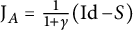
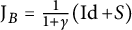
${\operatorname {J}}_{A} =\tfrac {1}{1+\gamma }( \operatorname {{ Id}}- S)$
and
${\operatorname {J}}_{B} =\tfrac {1}{1+\gamma }( \operatorname {{ Id}}+ S)$
. -
(iv)
${\operatorname {R}}_{A}=\tfrac {1}{1+\gamma }((1-\gamma )\operatorname {{ Id}}-2S)$
and
${\operatorname {R}}_{B}=\tfrac {1}{1+\gamma }((1-\gamma )\operatorname {{ Id}}+2S)$
. -
(v)
${\operatorname {R}}_{B}{\operatorname {R}}_{A}=\operatorname {{ Id}}$
. Hence,
$T=\operatorname {{ Id}}$
, and consequently,
$\operatorname {{ Id}}-T\equiv 0$
. -
(vi)
$\{0\}={\operatorname {ran}}\,(\operatorname {{ Id}}-T)=\overline {\operatorname {ran}}\,(\operatorname {{ Id}}-T)\subsetneqq X=\overline {D\cap R}$
.







Proof (i): This is clear. (ii): This follows from, for example, combining [Reference Bauschke and Combettes3, Example 20.53 and Proposition 25.11]. (iii): Indeed, observe that
 ${\operatorname {J}}_{A}{\operatorname {J}}_{B} =(\operatorname {{ Id}}+S)^{-1}(\operatorname {{ Id}}-S)^{-1} =((\operatorname {{ Id}}-S)(\operatorname {{ Id}}+S))^{-1} =((1+\gamma )\operatorname {{ Id}})^{-1} =(1+\gamma )^{-1}\operatorname {{ Id}}$
. Therefore,
 ${\operatorname {J}}_{A}=(1+\gamma )^{-1}(\operatorname {{ Id}}-S)$
and
 ${\operatorname {J}}_{B}=(1+\gamma )^{-1}(\operatorname {{ Id}}+S)$
, as claimed. (iv): This is a direct consequence of (iii). (v): Using (iv), we have
 ${\operatorname {R}}_{B}{\operatorname {R}}_{A} =(1+\gamma )^{-2}((1-\gamma )\operatorname {{ Id}}+2S)((1-\gamma )\operatorname {{ Id}}-2S) =(1+\gamma )^{-2}((1-\gamma )^2\operatorname {{ Id}}-4S^2) =(1+\gamma )^{-2}((1-\gamma )^2\operatorname {{ Id}}+4\gamma \operatorname {{ Id}})=\operatorname {{ Id}}$
. (vi): Clearly,
 $\operatorname {dom}\, A=\operatorname {dom}\, B=X$
. Moreover, by assumption,
 $A^{-1}=-B^{-1}=-\gamma ^{-1} S$
. Hence, A and
 $B $
are surjective, and we conclude that
 ${\operatorname {ran}}\, A={\operatorname {ran}}\, B=X$
. The conclusion follows.
Example 2.8 Suppose that
 $X=\mathbb R^2 $
. Let
 $u\in \mathbb R^2$
be such that
 $\lVert u\rVert =1$
. Let
 $A\colon \mathbb R^2\to \mathbb R^2\colon (\xi _1,\xi _2)\mapsto (-\xi _2,\xi _1)$
(the counterclockwise rotator in the plane by
 $\pi /2$
) and set
 $B=N_{\mathbb R\cdot u}$
. Then A is not
 $3^*$
monotone,
 ${\operatorname {J}}_{A}=\tfrac {1}{2}(\operatorname {{ Id}}-A)$
,
 ${\operatorname {R}}_{A} =-A$
and
 ${\operatorname {J}}_{B}={\operatorname {P}}_{\mathbb R\cdot u}=\left \langle {\cdot },{u} \right \rangle u$
. Moreover, the following hold:
-
(i)
$\operatorname {dom}\, A={\operatorname {ran}}\, A=\mathbb R^2$
,
$\operatorname {dom}\, B=\mathbb R\cdot u$
,
${\operatorname {ran}}\, B=\{ u\}^{\scriptscriptstyle \perp }$
. -
(ii)
$\overline {D\cap R}=D\cap R=\mathbb R^2$
. -
(iii)
$ \operatorname {{ Id}}-T= {\operatorname {P}}_{\mathbb R\cdot {\operatorname {J}}_{A} u} $
. -
(iv)
${\operatorname {ran}}\, (\operatorname {{ Id}}-T)=\overline {\operatorname {ran}}\,(\operatorname {{ Id}}-T)= \mathbb R\cdot {\operatorname {J}}_{A}u $
. -
(v)
$ \mathbb R\cdot {\operatorname {J}}_{A}u=\overline {\operatorname {ran}}\,(\operatorname {{ Id}}-T)\subsetneqq \overline {D\cap R}=\mathbb R^2$
.







Proof It is clear that A is not
 $3^*$
monotone (by applying Example 2.7(i) with S replaced by A), that
 $B=\partial \iota _{\mathbb R\cdot u}$
is
 $3^*$
monotone, that
 $\operatorname {dom}\, A={\operatorname {ran}}\, A=\mathbb R^2$
, and that
 $\operatorname {dom}\, B=\mathbb R\cdot u$
. The formulae for
 ${\operatorname {J}}_{A} $
and
 ${\operatorname {R}}_{A}$
follow from applying Example 2.7(iii)&(iv) with
 $\gamma =1$
. The formula for
 ${\operatorname {J}}_{B}$
follows from, for example, [Reference Bauschke and Combettes3, Example 23.4].
(i)&(ii): This is clear.
(iii): Set
 $u=(\alpha ,\beta )$
and observe that
 $\alpha ^2+\beta ^2=1$
. It is straightforward to verify that
 $$ \begin{align} {\operatorname{J}}_{B}={\operatorname{P}}_{\mathbb R\cdot u}=\left\langle{\cdot},{u} \right\rangle u =\begin{pmatrix} \alpha^2&\alpha \beta \\ \alpha \beta&\beta^2 \end{pmatrix} ~~\text{hence}~~ R_B =\begin{pmatrix} 2 \alpha^2-1&2\alpha \beta \\ 2 \alpha \beta&2\beta^2-1 \end{pmatrix}. \end{align} $$
On the one hand, we have
 $$ \begin{align} \operatorname{{ Id}}-T=\tfrac{1}{2}(\operatorname{{ Id}}-R_B{\operatorname{R}}_{A}) =\begin{pmatrix} \tfrac{1}{2}+\alpha \beta& \tfrac{1}{2}-\alpha^2 \\ -\tfrac{1}{2}+\beta^2&\tfrac{1}{2}-\alpha \beta \end{pmatrix} = \frac{1}{2}\begin{pmatrix} (\alpha +\beta)^2& -(\alpha^2-\beta^2) \\ -(\alpha^2-\beta^2)&(\alpha -\beta)^2 \end{pmatrix}. \end{align} $$
On the other hand, observe that  ; hence,
 $\lVert {\operatorname {J}}_{A}u\rVert ^2=\tfrac {1}{2}$
. Consequently,

and the conclusion follows.
(iv): This is a direct consequence of (iii). (v): Combine (ii) and (iv).
We conclude this section with the following example which shows in a strong way that the closures of the sets in Theorem 2.5 are critical.
Let U and V be nonempty closed convex subsets of X such that U is bounded. We recall that (see, for example, [Reference Bauschke and Combettes3, Proposition 3.42])
 $$ \begin{align} U+V \text{ is closed.} \end{align} $$
Example 2.9 Suppose that
 $\dim X\ge 2$
. Let
 $C=\operatorname {ball}(0;1)$
be the closed unit ball and let U be a closed linear subspace of X such that
 $U\neq \{0\}$
. Set
 $(A,B)=(N_C,N_U)$
. Then the following hold:
-
(i)
$(\operatorname {dom}\, A,\operatorname {dom}\, B,{\operatorname {ran}}\, A,{\operatorname {ran}}\, B)=(C,U,X,U^\perp )$
. -
(ii)
$\overline {\operatorname {dom}\, A-\operatorname {dom}\, B}=\overline {C+U}={C+U}=\operatorname {dom}\, A-\operatorname {dom}\, B$
. -
(iii)
$\overline {\operatorname {ran}}\, (\operatorname {{ Id}}-T)={C+U}$
. -
(iv) Set
$S=\big \{{u+u^{\scriptscriptstyle \perp }}~\big |~{u\in U\smallsetminus \{0\}, u^{\scriptscriptstyle \perp }\in U^\perp , \lVert u^{\scriptscriptstyle \perp }\rVert =1}\big \}$
. Then
$S\subseteq (C+U)\smallsetminus {\operatorname {ran}}\, (\operatorname {{ Id}}-T)$
. Consequently,
${\operatorname {ran}}\,(\operatorname {{ Id}}-T)\subsetneqq C+U=\operatorname {dom}\, A-\operatorname {dom}\, B$
.






Proof (i): This is clear in view of, for example, [Reference Bauschke and Combettes3, Corollary 21.25]. (ii): The first and the third identities follow from (i). The second identity follows from (33) applied with V replaced by C. (iii): Combine (i), (ii) and Theorem 2.5(iii). (iv): Clearly,
 $S\subseteq C+U$
. Now let
 $s\in S$
. Then
 $s=u+u^{\scriptscriptstyle \perp }, u\in U\smallsetminus \{0\}, u^{\scriptscriptstyle \perp }\in U^\perp , \lVert u^{\scriptscriptstyle \perp }\rVert =1$
. Suppose for eventual contradiction that
 $s\in {\operatorname {ran}}\,(\operatorname {{ Id}}-T)$
. Let
 $y\in X$
be such that
 $s=y-Ty$
. Because
 ${\operatorname {P}}_{U}$
is linear by, for example, [Reference Deutsch10, 5.13(1) on page 79], we have in view of (6),
 $$ \begin{align} u+u^{\scriptscriptstyle\perp}= {\operatorname{P}}_{C} y-2{\operatorname{P}}_{U}{\operatorname{P}}_{C}y+{\operatorname{P}}_{U}y. \end{align} $$
We proceed by examining the following cases.
Case 1:
 $y\in C$
. Then (34) yields
 $u+u^{\scriptscriptstyle \perp }= y-2{\operatorname {P}}_{U}y+{\operatorname {P}}_{U}y={\operatorname {P}}_{U^\perp }y\in U^\perp $
. That is,
 $u\in (-u^{\scriptscriptstyle \perp }+U^\perp )\cap U=U^\perp \cap U$
; hence,
 $u=0$
, which is absurd.
Case 2:
 $y\not \in C$
. In this case,
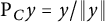 ${\operatorname {P}}_{C}y=y/\lVert y\rVert $
by, for example, [Reference Bauschke and Combettes3, Example 3.18]. Therefore, (34) yields
 $$ \begin{align} u+u^{\scriptscriptstyle\perp}= \frac{ 1}{\lVert y\rVert}y-2\frac{ 1}{\lVert y\rVert}{\operatorname{P}}_{U}y+{\operatorname{P}}_{U}y =\frac{ 1}{\lVert y\rVert}{\operatorname{P}}_{U^\perp}y+\Big(1-\frac{ 1}{\lVert y\rVert}\Big){\operatorname{P}}_{U}y. \end{align} $$
That is,
 $u^{\scriptscriptstyle \perp }={\operatorname {P}}_{U^\perp }y/\lVert y\rVert $
. On the one hand, this implies that
 $1=\lVert u^{\scriptscriptstyle \perp }\rVert =\lVert {\operatorname {P}}_{U^\perp }y\rVert /\lVert y\rVert $
. Therefore,
 $\lVert {\operatorname {P}}_{U^\perp }y\rVert ^2=\lVert y\rVert ^2=\lVert {\operatorname {P}}_{U}y\rVert ^2+\lVert {\operatorname {P}}_{U^\perp }y\rVert ^2$
. Hence,
 ${\operatorname {P}}_{U}y=0$
. On the other hand, (35) implies that
 $u=(1-(1/\lVert y\rVert )){\operatorname {P}}_{U}y$
. Altogether, we conclude that
 $u=0$
, which is absurd. Therefore,
 $s\not \in {\operatorname {ran}}\,(\operatorname {{ Id}}-T) $
. The proof is complete.
3 The case
$(A,B)=(\partial f,\partial g)$

In the remainder of this paper, we assume that

We use the abbreviations

In this case,
 $$ \begin{align} {\operatorname{T}}_{(\partial f, \partial g)}=\operatorname{{ Id}}-{\operatorname{J}}_{\partial f} +{\operatorname{J}}_{\partial g}{\operatorname{R}}_{\partial f}=\operatorname{{ Id}}-\operatorname{P}_f+\operatorname{P}_g{\operatorname{R}}_{f}. \end{align} $$
The following simple lemma is stated in [Reference Brezis and Haraux8, page 167]. We provide the short proof for the sake of completeness.
Lemma 3.1 Let
 $(y,z^*)\in \operatorname {dom}\, f\times \operatorname {dom}\, f^*$
. Then
 $$ \begin{align} \inf_{(x,x^*)\in \operatorname{gra} \partial f }\left\langle{x-y},{x^*-z^*} \right\rangle>-\infty. \end{align} $$
Consequently,
 $\partial f$
is
 $3^* $
monotone.
Proof Let
 $(x,x^*)\in \operatorname {gra} \partial f$
. It follows from the subgradient inequality that
 $(\forall y\in X)$
 $f(y)\ge f(x)+\left \langle {x^*},{y-x} \right \rangle =f(x)+\left \langle {x^*-z^*},{y-x} \right \rangle +\left \langle {z^*},{y-x} \right \rangle $
. Rearranging yields
 $$ \begin{align} \left\langle{x-y},{x^*-z^*} \right\rangle &\ge f(x)-f(y)-\left\langle{z^*},{x} \right\rangle+\left\langle{y},{z^*} \right\rangle \end{align} $$
 $$ \begin{align} &\qquad\qquad\qquad\qquad =-f(y)-(\left\langle{z^*},{x} \right\rangle-f(x))+\left\langle{y},{z^*} \right\rangle \ \end{align} $$
 $$ \begin{align} &\qquad\qquad\ \ \ge -f(y)-f^*(z^*)+\left\langle{y},{z^*} \right\rangle. \end{align} $$
This verifies (39). The
 $3^*$
monotonicity of
 $\partial f$
follows from combining (39) and the fact that
 $\operatorname {dom}\, \partial f \subseteq \operatorname {dom}\, f$
and
 $\operatorname {dom}\, \partial f^* \subseteq \operatorname {dom}\, f^*$
.
Proposition 3.2 Let
 $w\in ({\operatorname {dom}\,} f-{\operatorname {dom}\,} g)\cap ({\operatorname {dom}\,} f^*+{\operatorname {dom}\,} g^*)$
. Set
 $(A,B)=(\partial f,\partial g)$
. Then
 $w\in \overline {{\operatorname {ran}}\,} (\operatorname {{ Id}}-T)$
.
Proof Proceeding similar to the proof Proposition 2.4, let
 $(x_n)_{n\ge 1}$
be such that
 $(x_n, w-\tfrac {1}{n^2}x_n)_{n\ge 1}$
lies in
 $\operatorname {gra} (\operatorname {{ Id}}-T)$
. Our goal is to show that
 $$ \begin{align} \tfrac{1}{n^2}x_n\to 0. \end{align} $$
Obtain
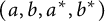 $(a,b,a^*,b^*)$
from
 $ \operatorname {dom}\, f\times \operatorname {dom}\, g\times \operatorname {dom}\, f^*\times \operatorname {dom}\, g^*$
such that
 $$ \begin{align} w=a-b=a^*+b^*. \end{align} $$
Recall that Lemma 2.1 and (42) imply 
 $$ \begin{align} \left\langle{x-(a+a^*)},{x-Tx -w} \right\rangle &\ge \left\langle{\operatorname{P}_fx-a},{\operatorname{P}_{f^*}x-a^*} \right\rangle +\left\langle{\operatorname{P}_g{\operatorname{R}}_{f}x-b},{\operatorname{P}_{g^*}{\operatorname{R}}_{f}x-b^*} \right\rangle. \end{align} $$
It follows from Lemma 3.1 applied to f and g, respectively, that
 $$ \begin{align} \inf_{x\in X}\left\langle{\operatorname{P}_fx-a},{\operatorname{P}_{f^*}x-a^*} \right\rangle>-\infty ~~\text{and}~~ \inf_{x\in X}\left\langle{\operatorname{P}_g{\operatorname{R}}_{A} x-b},{\operatorname{P}_{g^*}{\operatorname{R}}_{A}x-b^*} \right\rangle>-\infty. \end{align} $$
Combining (44) with (43) in view of (42), we learn that
 $$ \begin{align} &\qquad \inf_{x\in X}\left\langle{x-(a+a^*)},{x-Tx -(a-b)} \right\rangle \nonumber \\ &\ge \inf_{x\in X}\big(\left\langle{\operatorname{P}_fx-a},{\operatorname{P}_{f^*}x-a^*} \right\rangle +\left\langle{\operatorname{P}_g{\operatorname{R}}_{f} x-b},{\operatorname{P}_{g^*}{\operatorname{R}}_{f}x-b^*} \right\rangle\big)\qquad\quad \end{align} $$
 $$ \begin{align} &\ge \inf_{x\in X}\left\langle{\operatorname{P}_fx-a},{\operatorname{P}_{f^*}x-a^*} \right\rangle +\inf_{x\in X}\left\langle{\operatorname{P}_g{\operatorname{R}}_{f} x-b},{\operatorname{P}_{g^*}{\operatorname{R}}_{f}x-b^*} \right\rangle>-\infty. \end{align} $$
Now proceed similarly to the proof of Proposition 2.4(i) to conclude that
 $(x_n/n)_{n\ge 1}$
is bounded, and hence, (41) holds.
The following result further refines the formula obtained in Theorem 2.5 and Theorem 2.6 when the operators are subdifferential operators.
Theorem 3.3 Set
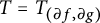 $T=T_{(\partial f,\partial g)}$
. Then the following hold:
-
(i)
$\overline {\operatorname {ran}}\, (\operatorname {{ Id}}-T) =\overline {(\operatorname {dom}\, f-\operatorname {dom}\, g) \cap (\operatorname {dom}\, f^*+\operatorname {dom}\, g^*)}$
. -
(ii)
$\overline {\operatorname {ran}}\, T=\overline {(\operatorname {dom}\, f-\operatorname {dom}\, g^*) \cap (\operatorname {dom}\, f^*+\operatorname {dom}\, g)}$
.


Proof (i): Indeed, by Proposition 3.2 and (10) applied with
 $(A,B)$
replaced with
 $(\partial f, \partial g)$
, we have
 $$ \begin{align} &\quad\overline{(\operatorname{dom}\, f-\operatorname{dom}\, g)\cap(\operatorname{dom}\, f^*+\operatorname{dom}\, g^*)}\qquad \end{align} $$
 $$ \begin{align} &\subseteq \overline{\operatorname{ran}}\,(\operatorname{{ Id}}-T)\qquad\qquad\qquad\qquad\qquad \qquad\qquad\end{align} $$
 $$ \begin{align} &\subseteq\overline{(\operatorname{dom}\, \partial f-\operatorname{dom}\,\partial g) \cap(\operatorname{dom}\,\partial f^*+\operatorname{dom}\,\partial g^*)} \end{align} $$
 $$ \begin{align} &\subseteq \overline{(\operatorname{dom}\, f-\operatorname{dom}\, g) \cap(\operatorname{dom}\, f^*+\operatorname{dom}\, g^*)}.\qquad \end{align} $$
(ii): Observe that
 $T=\operatorname {{ Id}}-T_{(\partial f,\partial g^*)}$
. Now combine with (i) applied with g replaced by
 $g^{*}$
. This completes the proof.
As a byproduct of the last proof, we obtain the following corollary.
Corollary 3.4 We have
 $$ \begin{align} &\overline{(\operatorname{dom}\, \partial f-\operatorname{dom}\,\partial g) \cap(\operatorname{dom}\,\partial f^*+\operatorname{dom}\,\partial g^*)} \nonumber \\ &\quad = \overline{(\operatorname{dom}\, f-\operatorname{dom}\, g) \cap(\operatorname{dom}\, f^*+\operatorname{dom}\, g^*)}. \end{align} $$
Proof This is a direct consequence of (46).
Example 3.5 Suppose that U and V are nonempty closed convex subsets of X. Set
 $f=\iota _U$
and
 $g=\iota _V$
. Suppose that U is bounded. Then the following hold:
-
(i)
$\overline {\operatorname {ran}}\,(\operatorname {{ Id}}-T)=U-V$
. -
(ii)
$\overline {\operatorname {ran}}\, T=U-(\operatorname {rec} V)^\ominus $
.


Proof Observe that
 $(\operatorname {dom}\, f, \operatorname {dom}\, g) =(\overline {\operatorname {dom}\,} f, \overline {\operatorname {dom}\,} g) =(U,V)$
. Moreover,
 $(\operatorname {dom}\, f^*,\overline {\operatorname {dom}\,} g^* )=(X, (\operatorname {rec} V)^\ominus )$
. (i): It follows from Theorem 3.3(i) that
 $\overline {\operatorname {ran}}\,(\operatorname {{ Id}}-T)=\overline {(U-V)\cap X} =\overline {U-V}$
. Now combine with (33) applied with V replaced by
 $-V$
. (ii): It follows from Theorem 3.3(ii) that
 $\overline {\operatorname {ran}}\, T=\overline {\operatorname {dom}\, f -\operatorname {dom}\, g^*} =\overline {\overline {\operatorname {dom}\,} f -\overline {\operatorname {dom}\,} g^*} =\overline {U-(\operatorname {rec} V)^\ominus } $
. Now combine with (33) applied with V replaced by
 $-(\operatorname {rec} V)^\ominus $
.
4 The sets D and R and their corresponding minimal norm vectors
Because A, B, and
 $\operatorname {{ Id}}-T$
are maximally monotone, we know that the sets
 $\operatorname {dom}\, A$
,
 $\operatorname {dom}\, B$
,
 ${\operatorname {ran}}\, A$
,
 ${\operatorname {ran}}\, B$
, and
 ${\operatorname {ran}}\, (\operatorname {{ Id}}-T)$
have convex closures (see [Reference Simons20, Theorem 31.2]); that is,
 $$ \begin{align} \overline{D}, \overline{R} \text{ and } \overline{\operatorname{ran}}\,(\operatorname{{ Id}}-T) \text{ are convex. } \end{align} $$
Consequently, the following vectors
 $$ \begin{align} v= P_{\overline{\operatorname{ran}}\, (\operatorname{{ Id}}-T)}(0), \quad v_D= P_{\overline{\operatorname{dom}\, A-\operatorname{dom}\, B}}(0), \quad v_R= P_{\overline{{\operatorname{ran}}\, A+{\operatorname{ran}}\, B}} (0) \end{align} $$
are well defined.
Remark 4.1
-
(i) If X is finite-dimensional, then we know more (see, for example, [Reference Bauschke, Hare and Moursi5, Lemma 5.1(i)]): D and R are nearly convexFootnote 2 ; so in particular, by [Reference Bauschke, Moffat and Wang6, Theorem 2.16],
$\overline {D} = \overline {\operatorname {ri} D}$
and
$\overline {R} = \overline {\operatorname {ri} R}$
. Moreover, Minty’s theorem applied to B yields
$\operatorname {ri} D-\operatorname {ri} R=\operatorname {ri} (D-R)=\operatorname {ri} (\operatorname {dom}\, A-\operatorname {dom}\, B-{\operatorname {ran}}\, A-{\operatorname {ran}}\, B)=\operatorname {ri} X=X$
. Hence,
$\operatorname {ri} D \cap \operatorname {ri} R\neq \varnothing $
. Consequently, in view of [Reference Bauschke, Hare and Moursi5, Lemma 3.9(iv)], we learn that (50)
$$ \begin{align} \overline{D\cap R}=\overline{D}\cap \overline{R}. \end{align} $$
-
(ii) We do not know whether or not the identity (50) survives in infinite-dimensional Hilbert spaces. Indeed, in view of Theorem 4.2 below, on the one hand, any counterexample must feature that neither of the operators is an affine relation or that none of the operators has a bounded domain or a bounded range. On the other hand, Theorem 4.4 implies that one has to avoid scenarios when both D and R has a nonempty interior.





The next result provides some sufficient conditions where (50) holds in infinite-dimensional Hilbert spaces.
Theorem 4.2 Suppose that one of the following conditions holds:
-
(i)
$(\exists C\in \{A,B\})$
such that
$\operatorname {dom}\, C$
and
${\operatorname {ran}}\, C$
are affine. -
(ii)
$(A,B)=(N_K,N_L)$
, where K and L are nonempty closed convex cones of X and
$K^\ominus +L^\ominus $
is closed. -
(iii)
$(\exists C\in \{A,B\})$
$\operatorname {dom}\, C$
is bounded or
${\operatorname {ran}}\, C$
is bounded. -
(iv)
$(\exists C\in \{A,B\})$
$\operatorname {dom}\, C=X$
or
${\operatorname {ran}}\, C=X$
.






Then
 $\overline {D\cap R}=\overline {D}\cap \overline {R}$
.
Proof It is obvious that
 $\overline {D\cap R}\subseteq \overline {D}\cap \overline {R}$
. Therefore, we only need to verify that
 $\overline {D}\cap \overline {R}\subseteq \overline {D\cap R}$
. (i): Indeed, suppose that
 $C=A$
. Let
 $w\in \overline {D}\cap \overline {R}$
and let
 $(a_n,b_n,a_n^*,b_n^*)_{n\in {\mathbb N}}$
be a sequence in
 $\operatorname {dom}\, A\times \operatorname {dom}\, B\times {\operatorname {ran}}\, A\times {\operatorname {ran}}\, B$
such that
 $a_n-b_n\to w$
and
 $a_n^*+b_n^*\to w$
. Set
 $(\forall {n\in {\mathbb N}})$
 $w_n= {\operatorname {J}}_{A} (a_n^*+b_n^*)+{\operatorname {J}}_{A^{-1}}(a_n-b_n)$
. Because
 ${\operatorname {J}}_{A}$
, as is
 ${\operatorname {J}}_{A^{-1}}$
, is firmly nonexpansive, it is continuous. Therefore,
 $$ \begin{align} w_n\to {\operatorname{J}}_{A} w+{\operatorname{J}}_{A^{-1}}w=w. \end{align} $$
We claim that
 $$ \begin{align} (w_n)_{n\in{\mathbb N}} \text{ lies in } D\cap R. \end{align} $$
Indeed, on the one hand, because
 $\operatorname {dom}\, A={\operatorname {ran}}\, {\operatorname {J}}_{A}$
is affine, we have
 $$ \begin{align} w_n &= {\operatorname{J}}_{A} (a_n^*+b_n^*)+a_n-b_n-{\operatorname{J}}_{A}(a_n-b_n)\qquad\qquad\qquad\qquad \qquad \ \end{align} $$
 $$ \begin{align} &\ \ ={\operatorname{J}}_{A} (a_n^*+b_n^*)+a_n-{\operatorname{J}}_{A} (a_n-b_n)-b_n \in \operatorname{dom}\, A-\operatorname{dom}\, B=D. \end{align} $$
On the other hand, because
 ${\operatorname {ran}}\, A={\operatorname {ran}}\, {\operatorname {J}}_{A^{-1}}$
is affine, we have
 $$ \begin{align} w_n &= {\operatorname{J}}_{A^{-1}} (a_n-b_n)+a_n^*+b_n^*-{\operatorname{J}}_{A^{-1}} (a_n^*+b_n^*) \quad\qquad\qquad\qquad\qquad\end{align} $$
 $$ \begin{align} &\ ={\operatorname{J}}_{A^{-1}} (a_n-b_n)+a^*_n-{\operatorname{J}}_{A^{-1}}(a_n^*+b_n^*)+b^*_n \in {\operatorname{ran}}\, A+{\operatorname{ran}}\, B=R. \end{align} $$
This proves (52). Now combine with (51). The proof in the case
 $C=B$
is similar.
(ii): Let
 $w\in \overline {D}\cap \overline {R}=\overline {(K-L)}\cap ({K^\ominus +L^\ominus })$
and let
 $(k_n,l_n)_{n\in {\mathbb N}}$
be a sequence in
 $K\times L $
such that
 $ k_n-l_n\to w$
. Set
 $(\forall {n\in {\mathbb N}})$
 $w_n= {\operatorname {P}}_{(K\cap L)^\ominus }(k_n-l_n)$
. Observe that because
 $(K\cap L)^\ominus =\overline {K^\ominus +L^\ominus }=K^\ominus +L^\ominus $
by, for example, [Reference Deutsch10, remarks on page 48], we have
 $$ \begin{align} w_n\to {\operatorname{P}}_{(K\cap L)^\ominus}w=w. \end{align} $$
On the one hand, by construction,
 $(w_n)_{n\in {\mathbb N}}$
lies in
 . On the other hand, we have
 $(\forall {n\in {\mathbb N}})$
 Hence,
 $(w_n)_{n\in {\mathbb N}}$
lies in
 . Combining this with (55), we learn that
 $w\in \overline {({K-L})\cap ({K^\ominus +L^\ominus })}$
. (iii): If
 $\operatorname {dom}\, C$
is bounded, then [Reference Bauschke and Combettes3, Corollary 21.25] implies that
 ${\operatorname {ran}}\, C=X$
; hence,
 $R=X$
. Therefore,
 $\overline {D\cap R}=\overline {D}=\overline {D}\cap X =\overline {D}\cap \overline {R}$
. The case when
 ${\operatorname {ran}}\, C$
is bounded follows similarly by applying the previous argument to
 $C^{-1}$
. (iv): If
 $\operatorname {dom}\, C=X$
, then
 $D=X$
. Therefore,
 $\overline {D\cap R}=\overline {R}=X\cap \overline {R} =\overline {D}\cap \overline {R}$
. The case when
 ${\operatorname {ran}}\, C=X$
follows similarly.
Before we proceed, we recall the following facts.
Fact 4.3 (Simons)
Suppose that
 $\operatorname {int} D\neq \varnothing $
. Then
 $\overline {D}=\overline {\operatorname {int} D}$
.
Proof See [Reference Simons19, Theorem 22.1(c) and Theorem 22.2(a)].
When the sets D and R are reasonably fat – namely, when
 $\operatorname {int} D\neq \varnothing $
and
 $\operatorname {int} R\neq \varnothing $
– we obtain another sufficient condition for the conclusion
 $\overline {D\cap R}=\overline {D}\cap \overline {R}$
as we see in Theorem 4.4 below.
Theorem 4.4 Suppose that A and B are
 $3^*$
monotone. Suppose that
 $\operatorname {int} D\neq \varnothing $
and
 $\operatorname {int} R\neq \varnothing $
. Then
 $\overline {D\cap R}=\overline {D}\cap \overline {R}$
.
Proof It follows from Fact 4.3 applied to
 $(A, B)$
(respectively
 ) that
 $\overline {D}=\overline {\operatorname {int} D} $
(respectively
 $\overline {R}=\overline {\operatorname {int} R} $
). Let
 $w\in \overline {D}\cap \overline {R}$
. By Fact 4.3,
 $\overline {D}\cap \overline {R}=\overline {\operatorname {int} D}\cap \overline {\operatorname {int} R}$
; hence,
 $w\in \overline {\operatorname {int} D}\cap \overline {\operatorname {int} R}$
, and therefore,
 $$ \begin{align} \text{there exists a sequence } (d_n,r_n)_{n\in{\mathbb N}} \text{ in } {\operatorname{int} D}\times{\operatorname{int} R} \text{ such that } (d_n,r_n )\to (w,w). \end{align} $$
Observe that (56) implies that
 $(\forall {n\in {\mathbb N}})$
 $0\in \operatorname {int}(\operatorname {dom}\, A-(d_n+\operatorname {dom}\, B))=\operatorname {int}(\operatorname {dom}\, A-\operatorname {dom}\, B(\cdot -d_n))$
. Therefore, by, for example, [Reference Bauschke and Combettes3, Corollary 25.5(iii)], we learn that
 $(\forall {n\in {\mathbb N}})$
 $A+B(\cdot -d_n)$
is maximally monotone. On the one hand, it follows from the
 $3^*$
monotonicity of A and B in view of the celebrated Brezis–Haraux theorem (see [Reference Brezis and Haraux8, Théorème 3] and also [Reference Simons20, Corollary 31.6]) that
 $(\forall {n\in {\mathbb N}})$
 $$ \begin{align} r_n&\in \operatorname{int} ({\operatorname{ran}}\, A+{\operatorname{ran}}\, B)=\operatorname{int} ({\operatorname{ran}}\, A+{\operatorname{ran}}\, B(\cdot -d_n)) \qquad\qquad\qquad\qquad\end{align} $$
 $$ \begin{align} &\qquad =\operatorname{int} {\operatorname{ran}}\, (A+B(\cdot -d_n)). \end{align} $$
Therefore, there exists a sequence
 $((x_n,u_n))_{n\in {\mathbb N}}$
in
 $ \operatorname {gra} A$
and
 $(x_n-d_n,-u_n+r_n )_{n\in {\mathbb N}}$
in
 $ \operatorname {gra} B$
. Using Minty’s theorem Fact 1.1, we rewrite this as
 $$ \begin{align} (x_n,u_n)&=({\operatorname{J}}_{A} (x_n+u_n),{\operatorname{J}}_{A^{-1}}(x_n+u_n)) \quad\end{align} $$
 $$ \begin{align} (x_n-d_n,-u_n+r_n)&=({\operatorname{J}}_{B}(x_n-u_n-d_n+r_n),{\operatorname{J}}_{B^{-1}}(x_n-u_n-d_n+r_n)). \end{align} $$
It follows from (58) that
 $$ \begin{align} d_n&={\operatorname{J}}_{A} (x_n+u_n)-{\operatorname{J}}_{B}(x_n-u_n-d_n+r_n)\quad \ \ \end{align} $$
 $$ \begin{align} r_n&={\operatorname{J}}_{A^{-1}}(x_n+u_n)+{\operatorname{J}}_{B^{-1}}(x_n-u_n-d_n+r_n). \end{align} $$
Now, set
 $(\forall {n\in {\mathbb N}})$
 $$ \begin{align} z_n= {\operatorname{J}}_{A} (x_n+u_n)-{\operatorname{J}}_{B}{\operatorname{R}}_{A}(x_n+u_n)\in {\operatorname{ran}}\, (\operatorname{{ Id}}-T). \end{align} $$
We claim that
 $(\forall {n\in {\mathbb N}})$
 $$ \begin{align} \lVert z_n-r_n\rVert^2+ \lVert z_n-d_n\rVert^2\le \lVert d_n-r_n\rVert^2. \end{align} $$
Indeed, using (60), (59b), the firm nonexpansiveness of
 $J_{B^{-1}}$
, (58), (60), and (59a), we obtain
 $$ \begin{align} \lVert z_n-r_n\rVert^2 &=\lVert{\operatorname{J}}_{A} (x_n+u_n)-{\operatorname{J}}_{B}{\operatorname{R}}_{A}(x_n+u_n)- {\operatorname{J}}_{A^{-1}}(x_n+u_n) \qquad\qquad\qquad\qquad\nonumber\\ &\quad -{\operatorname{J}}_{B^{-1}}(x_n-u_n-d_n+r_n)\rVert^2 \end{align} $$
 $$ \begin{align} &=\lVert{\operatorname{J}}_{B^{-1}}{\operatorname{R}}_{A}(x_n+u_n)-{\operatorname{J}}_{B^{-1}}(x_n-u_n-d_n+r_n)\rVert^2 \qquad\qquad\qquad \; \; \end{align} $$
 $$ \begin{align} &\le \lVert{\operatorname{R}}_{A}(x_n+u_n)-(x_n-u_n-d_n+r_n)\rVert^2 \nonumber \\ &\quad-\lVert{\operatorname{J}}_{B}{\operatorname{R}}_{A}(x_n+u_n)-{\operatorname{J}}_{B}(x_n-u_n-d_n+r_n)\rVert^2 \qquad\qquad\quad\end{align} $$
 $$ \begin{align} &= \lVert(x_n-u_n)-(x_n-u_n-d_n+r_n)\rVert^2- \lVert(x_n-z_n)-(x_n-d_n)\rVert^2 \end{align} $$
 $$ \begin{align} &= \lVert d_n-r_n\rVert^2- \lVert d_n-z_n\rVert^2.\qquad\qquad\qquad\qquad\qquad\qquad\quad\;\; \end{align} $$
This proves (61). Taking the limit as
 $n\to \infty $
in (61) in view of (56), we learn that
 $z_n\to w$
. Therefore, in view of (60), we learn that
 $w\in \overline {\operatorname {ran}}\,(\operatorname {{ Id}}-T)$
. Hence,
 $\overline {D}\cap \overline {R}\subseteq \overline {\operatorname {ran}}\,(\operatorname {{ Id}}-T)$
. Now combine this with (10) and recall that
 $\overline {D\cap R}\subseteq \overline {D}\cap \overline {R}$
. The proof is complete.
5 The vectors v,
$v_D$
and
$v_R$


We now turn to the minimal norm vectors in the sets
 $\overline {D}$
,
 $\overline {R}$
, and
 $\overline {\operatorname {ran}}\,(\operatorname {{ Id}}-T)$
– namely,
 $v_D$
,
 $v_R$
, and v, respectively. Before we proceed, we recall the following useful facts.
Fact 5.1 Let U and V be nonempty closed convex subsets of X. Then
 $$ \begin{align} {\operatorname{P}}_{\overline{U-V}}(0)\in\overline{({\operatorname{P}}_{U}-\operatorname{{ Id}})(V)}\cap\overline{(\operatorname{{ Id}}-{\operatorname{P}}_{V})(U)} \subseteq (-\operatorname{rec} U)^\ominus \cap(\operatorname{rec} V)^\ominus. \end{align} $$
Proof This follows from [Reference Bauschke and Borwein2, Corollary 4.6] and [Reference Zarantonello21, Theorem 3.1].
Fact 5.2 Let
 $A\colon X\rightrightarrows X$
be maximally monotone. Then the following hold:
-
(i)
$(\operatorname {rec} \overline {\operatorname {dom}}\, \ A)^\ominus \subseteq \operatorname {rec} (\overline {\operatorname {ran}}\, A)$
. -
(ii)
$(\operatorname {rec} {\overline {\operatorname {ran}}\,}\ A)^\ominus \subseteq \operatorname {rec} (\overline {\operatorname {dom}}\, \ A)$
.


Proof See [Reference Bauschke and Moursi7, Lemma 3.2]
Lemma 5.3 Let
 $S_1$
and
 $S_2$
be nonempty closed convex subsets of X and set
 $(\forall i\in \{1,2\})$
 $v_i=P_{S_i}(0)$
. Suppose that
 $\left \langle {v_1},{v_2} \right \rangle \le 0$
and that
 $v_1+v_2\in S_1\cap S_2$
. Then
 $v_1+v_2=P_{S_1\cap S_2}(0)$
.
Proof Let
 $s\in S_1\cap S_2$
. In view of the projection theorem – see, for example, [Reference Bauschke and Combettes3, Theorem 3.16] – it suffices to show that
 $(\forall s\in S_1\cap S_2)$
 $\left \langle {v_1+v_2-0},{v_1+v_2-s} \right \rangle \le 0$
. Indeed, we have
 $ \left \langle {v_1+v_2-0},{v_1+v_2-s} \right \rangle =\left \langle {v_1},{v_1+v_2-s} \right \rangle +\left \langle {v_2},{v_1+v_2-s} \right \rangle \le \left \langle {v_1},{v_1-s} \right \rangle +\left \langle {v_2},{v_2-s} \right \rangle \le 0+0=0. $
Parts of the following proposition were proved in [Reference Bauschke and Moursi7]. We reiterate the short proof for the sake of completeness and to avoid any confusion with the standing assumptions in [Reference Bauschke and Moursi7].
Proposition 5.4 The following hold:
-
(i)
$v_D\in (-\operatorname {rec} \overline {\operatorname {dom}}\, A)^\ominus \cap (\operatorname {rec} \overline {\operatorname {dom}}\, B)^\ominus =(-(\operatorname {rec} \overline {\operatorname {dom}}\, A)^\ominus )\cap (\operatorname {rec} \overline {\operatorname {dom}}\, B)^\ominus $
. -
(ii)
$v_R\in (-\operatorname {rec} \overline {\operatorname {ran}}\, A)^\ominus \cap (-\operatorname {rec} \overline {\operatorname {ran}}\, B)^\ominus =-((\operatorname {rec} \overline {\operatorname {ran}}\, A)^\ominus \cap (\operatorname {rec} \overline {\operatorname {ran}}\, B)^\ominus )$
. -
(iii)
$v_D\in (-\operatorname {rec} \overline {\operatorname {ran}}\, A)\cap (\operatorname {rec} \overline {\operatorname {ran}}\, B)$
. -
(iv)
$v_R\in (-\operatorname {rec} \overline {\operatorname {dom}}\, A)\cap (-\operatorname {rec} \overline {\operatorname {dom}}\, B) =-(\operatorname {rec} \overline {\operatorname {dom}}\, A\cap \operatorname {rec} \overline {\operatorname {dom}}\, B)$
. -
(v)
$\left \langle {v_D},{v_R} \right \rangle =0$
. -
(vi)
$v_D+v_R\in \overline {D}\cap \overline {R}$
. -
(vii)
$v_D+v_R={\operatorname {P}}_{\overline {D}\cap \overline {R}}(0)$
.







Proof (i)&(ii): Apply Fact 5.1 with
 $(U,V)$
replaced by
 $(\overline {\operatorname {dom}}\, A,\overline {\operatorname {dom}}\, B)$
(respectively
 $(\overline {\operatorname {ran}}\, A,-\overline {\operatorname {ran}}\, B)$
).
(iii)&(iv): Combine (i) (respectively (ii)) and Fact 5.2(i) (respectively Fact 5.2(ii)).
(v): It follows from (i) and (iv) that
 $(-v_D,-v_R)\in (\operatorname {rec}\overline {\operatorname {dom}}\, A)^\ominus \times \operatorname {rec}\overline {\operatorname {dom}}\, A$
. Hence,
 $\left \langle {v_D},{v_R} \right \rangle =\left \langle {-v_D},{-v_R} \right \rangle \le 0$
. Similarly, (iii) and (ii) imply that
 $(v_D,-v_R)\in \operatorname {rec}\overline {\operatorname {ran}}\, B\times (\operatorname {rec}\overline {\operatorname {ran}}\, B)^\ominus $
. Hence,
 $-\left \langle {v_D},{v_R} \right \rangle =\left \langle {v_D},{-v_R} \right \rangle \le 0$
. Altogether,
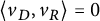 $\left \langle {v_D},{v_R} \right \rangle =0$
. (vi): Indeed, in view of (iv), we have
 $-v_R\in \operatorname {rec} \overline {\operatorname {dom}}\, B$
. Therefore,
 ${v_D}\ {+}\ {v_R}\ {\in}\ \overline {\operatorname {dom}\, A\ {-}\ \operatorname {dom}\, B}\ {+}\ {v_R}\ {=}\ \overline {\operatorname {dom}\, A-(-v_R\ {+}\ \overline {\operatorname {dom}}\, B)} \subseteq \overline {\operatorname {dom}\, A-\overline {\operatorname {dom}}\, B} = \overline {\operatorname {dom}\, A-\operatorname {dom}\, B}$
. Similarly, in view of (iii), we have
 $v_D\in \operatorname {rec} \overline {\operatorname {ran}}\, B$
. Therefore,
 ${v_D}+{v_R} \in \overline {{\operatorname {ran}}\, A+v_D+\overline {\operatorname {ran}}\, B} \subseteq \overline {{\operatorname {ran}}\, A+\overline {\operatorname {ran}}\, B} = \overline {{\operatorname {ran}}\, A+{{\operatorname {ran}}\,} B} $
. (vii): Combine (v), (vi), and Lemma 5.3 applied with
 $(S_1,S_2,v_1,v_2)$
replaced by
 $(\overline {D},\overline {R},v_D,v_R)$
.
Before we proceed, we recall the following useful fact.
Fact 5.5 Let C be a nonempty closed convex subset of X and let
 $w=P_C(0)$
. Suppose that
 $(u_n)_{n\in {\mathbb N}}$
is a sequence in C such that
 $\lVert u_n\rVert \to \lVert w\rVert $
. Then
 $u_n\to w$
.
Proof See [Reference Pazy15, Lemma 2].
Lemma 5.6 Suppose that
 $\overline {\operatorname {ran}}\,(\operatorname {{ Id}}-T)=\overline {D\cap R }$
(see Theorem 2.5 for sufficient conditions). Then we have
-
(i)
$v=v_D+v_R \Leftrightarrow v_D+v_R\in \overline {D\cap R} $
. -
(ii) Suppose
$ \overline {D\cap R} = \overline {D} \cap \overline {R} $
. Then
$v=v_D+v_R$
.



Proof (i): “
 $\Rightarrow $
”: This is clear in view of (49). “
 $\Leftarrow $
”: Observe that (11) implies that
 $\lVert v\rVert \le \lVert v_D+v_R\rVert $
. It follows from Proposition 5.4(v), the definition of
 $v_D$
that
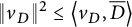 $\lVert v_D\rVert ^2\le \left \langle {v_D},{\overline {D}} \right \rangle $
; hence,
 $\lVert v_D\rVert ^2\le \left \langle {v_D},{\overline {D}\cap \overline {R}} \right \rangle $
. Similarly,
 $\lVert v_R\rVert ^2\le \left \langle {v_R},{\overline {D}\cap \overline {R}} \right \rangle $
. Therefore, using Cauchy–Schwarz and Proposition 5.4(v), we learn that
 $\lVert v_D+v_R\rVert ^2 =\lVert v_D\rVert ^2+\lVert v_R\rVert ^2 \le \left \langle {v},{v_D} \right \rangle +\left \langle {v},{v_R} \right \rangle =\left \langle {v},{v_D+v_R} \right \rangle \le \lVert v\rVert \lVert v_D+v_R\rVert $
. Hence,
 $\lVert v_D+v_R\rVert \le \lVert v\rVert $
. Altogether,
 $\lVert v\rVert =\lVert v_D+v_R\rVert $
. In view of (11) and Fact 5.5, we learn that
 $v=v_D+v_R$
. (ii): Combine (i) and Proposition 5.4(vii).
Proposition 5.7 Suppose that U and V are nonempty closed convex subsets of X. Set
 $(A,B)=(N_U,N_V)$
. Then the following hold:
-
(i)
$v_R=0$
. -
(ii)
$v_D=v$
. -
(iii)
$v=v_D+v_R$
.


Proof (i): If follows from [Reference Zarantonello21, Theorem 3.1] that
 $(\overline {{\operatorname {ran}}\, }A,\overline {{\operatorname {ran}}\,} B)=((\operatorname {rec} U)^\ominus ,(\operatorname {rec} V)^\ominus )$
. Therefore,
 $0\in (\operatorname {rec} U)^\ominus +(\operatorname {rec} V)^\ominus \subseteq \overline {R} $
. Hence,
 $v_R=0$
.
(ii): This is [Reference Bauschke, Hare and Moursi4, Proposition 3.5].
(iii): Combine (i) and (ii).
Corollary 5.8 Suppose that
 $\overline {\operatorname {ran}}\,(\operatorname {{ Id}}-T)=\overline {D\cap R }$
(see Theorem 2.5 for sufficient conditions). Suppose additionally that one of the following holds:
-
(i)
$\overline {D\cap R}=\overline {D}\cap \overline {R}$
. -
(ii) X is finite-dimensional.
-
(iii)
$(\exists C\in \{A,B\})$
such that
$\operatorname {dom}\, C$
and
${\operatorname {ran}}\, C$
are affine. -
(iv)
$(\exists C\in \{A,B\})$
such that
$\operatorname {dom}\, C=X$
or
${\operatorname {ran}}\, C=X$
. -
(v)
$(\exists C\in \{A,B\})$
$\operatorname {dom}\, C$
is bounded or
${\operatorname {ran}}\, C$
is bounded. -
(vi)
$A $
and B are
$3^*$
monotone,
$\operatorname {int} D\neq \varnothing $
and
$\operatorname {int} R\neq \varnothing $
. -
(vii)
$(A,B)=(N_U,N_V)$
, U and V are nonempty closed subsets of X.










Then
 $v=v_D+v_R$
.
Proof (i): This is Lemma 5.6(ii). (ii): This follows from combining Remark 4.1(i) and (i). (iii)–(v): Combine Theorem 4.2(i)–(iv) and Lemma 5.6(ii). (vi): Combine (i) and Theorem 4.4. (vii): This is Proposition 5.7(iii).
Remark 5.9 The minimal displacement vector in
 $\overline {\operatorname {ran}}\,(\operatorname {{ Id}}-T) $
can be found via (see [Reference Baillon, Bruck and Reich1], [Reference Bruck and Reich9], and [Reference Pazy15])
 $$ \begin{align} (\forall x\in X)\qquad v=-\lim_{n\to \infty}\frac{T^n x}{n} =\lim_{n\to \infty}T^n x-T^{n+1}x. \end{align} $$
Working in
 $X\times X$
and recalling (49), we observe that (see [Reference Bauschke and Combettes3, Proposition 29.4])
 $$ \begin{align} (v_R,v_D)=P_{\overline{R}\times \overline{D}}(0). \end{align} $$
Theorem 5.10 (computing
$v_D$
and
$v_R$
)


Suppose that one of the following holds:
-
(i)
$\overline {D\cap R}=\overline {D}\cap \overline {R}$
. -
(ii) X is finite-dimensional.
-
(iii)
$(\exists C\in \{A,B\})$
such that
$\operatorname {dom}\, C$
and
${\operatorname {ran}}\, C$
are affine. -
(iv)
$(\exists C\in \{A,B\})$
such that
$\operatorname {dom}\, C=X$
or
${\operatorname {ran}}\, C=X$
. -
(vi)
$(\exists C\in \{A,B\})$
$\operatorname {dom}\, C$
is bounded or
${\operatorname {ran}}\, C$
is bounded. -
(vii)
$A $
and B are
$3^*$
monotone,
$\operatorname {int} D\neq \varnothing $
and
$\operatorname {int} R\neq \varnothing $
. -
(viii)
$(A,B)=(N_U,N_V)$
, U and V are nonempty closed subsets of X.








Then
 $v=v_D+v_R$
. Let
 $x\in X$
. Then we have
 $$ \begin{align} \qquad v_R&=-\lim_{n\to \infty}\frac{{\operatorname{J}}_{A} T^n x}{n} =\lim_{n\to \infty}({\operatorname{J}}_{A} T^n x-{\operatorname{J}}_{A} T^{n+1}x)\qquad\qquad \end{align} $$
 $$ \begin{align} v_D&=-\lim_{n\to \infty}\frac{{\operatorname{J}}_{A^{-1}}T^n x}{n} =\lim_{n\to \infty}({\operatorname{J}}_{A^{-1}}T^n x-{\operatorname{J}}_{A^{-1}}T^{n+1}x). \end{align} $$
Proof The identity
 $v=v_D+v_R$
follows from Corollary 5.8. We now turn to (66). First we verify that
 $$ \begin{align} {\operatorname{ran}}\, ({\operatorname{J}}_{A} -{\operatorname{J}}_{A} T)\subseteq\overline{R} ~~\text{ and }~~{\operatorname{ran}}\, ({\operatorname{J}}_{A^{-1}}-{\operatorname{J}}_{A^{-1}}T)\subseteq\overline{D}. \end{align} $$
Indeed, observe that
 ${\operatorname {J}}_{A} T\ {+}\ {\operatorname {J}}_{A^{-1}}T\ {=}\ T\ {=}\ \operatorname {{ Id}}\ {-}\ {\operatorname {J}}_{A} \ {+}\ {\operatorname {J}}_{B}{\operatorname {R}}_{A}\ {=}\ {\operatorname {J}}_{A}\ {-}\ {\operatorname {R}}_{A}\ {+}\ {\operatorname {J}}_{B}{\operatorname {R}}_{A} ={\operatorname {J}}_{A} -{\operatorname {J}}_{B^{-1}}{\operatorname {R}}_{A}$
. Hence,
 ${\operatorname {J}}_{A} -{\operatorname {J}}_{A} T={\operatorname {J}}_{A^{-1}}T+{\operatorname {J}}_{B^{-1}}{\operatorname {R}}_{A}$
. Consequently,
 ${\operatorname {ran}}\, ({\operatorname {J}}_{A} -{\operatorname {J}}_{A} T)\subseteq {\operatorname {ran}}\, A+{\operatorname {ran}}\, B\subseteq \overline {R}$
. Similarly, we show that
 ${\operatorname {ran}}\, ({\operatorname {J}}_{A^{-1}}-{\operatorname {J}}_{A^{-1}}T)\subseteq \overline {D}$
. This verifies (67). Now let
 $x\in X$
, let
 $ n\ge 1$
, and observe that (67) and the convexity of
 $\overline {D}$
and
 $\overline {R}$
(see (48)) imply
 $$ \begin{align} & \{({\operatorname{J}}_{A}T^n x-{\operatorname{J}}_{A} T^{n+1} x,{\operatorname{J}}_{A^{-1}}T^nx-{\operatorname{J}}_{A^{-1}}T^{n+1} x ), \tfrac{1}{n}({\operatorname{J}}_{A} x-{\operatorname{J}}_{A} T^n x,{\operatorname{J}}_{A^{-1}}x-{\operatorname{J}}_{A^{-1}}T^n x ) \} \nonumber \\ &\quad \subseteq \overline{R}\times \overline{D}. \end{align} $$
Now, Proposition 5.4(v), (65), (68), the firm nonexpansiveness of
 ${\operatorname {J}}_{A}$
, and (64) yield
 $$ \begin{align} \lVert v_R+v_D\rVert^2 &=\lVert v_R\rVert^2+\lVert v_D\rVert^2 \end{align} $$
 $$ \begin{align} &=\lVert(v_R,v_D)\rVert^2\le \lVert\tfrac{1}{n}({\operatorname{J}}_{A} x-{\operatorname{J}}_{A} T^n x,{\operatorname{J}}_{A^{-1}}x-{\operatorname{J}}_{A^{-1}}T^n x )\rVert^2 \end{align} $$
 $$ \begin{align} &= \tfrac{1}{n^2}\lVert{\operatorname{J}}_{A} x-{\operatorname{J}}_{A} T^n x\rVert^2+\tfrac{1}{n^2}\lVert{\operatorname{J}}_{A^{-1}}x-{\operatorname{J}}_{A^{-1}}T^n x \rVert^2 \le \tfrac{1}{n^2}\lVert(x-T^n x)\rVert^2 \end{align} $$
 $$ \begin{align} &=\lVert\tfrac{1}{n}(x-T^n x)\rVert^2\to \lVert v\rVert^2=\lVert v_R+v_D\rVert^2, \end{align} $$
and
 $$ \begin{align} \lVert v_R+v_D\rVert^2 &=\lVert v_R\rVert^2+\lVert v_D\rVert^2 \end{align} $$
 $$ \begin{align} &=\lVert(v_R,v_D)\rVert^2\le \lVert({\operatorname{J}}_{A} T^nx-{\operatorname{J}}_{A} T^{n+1} x,{\operatorname{J}}_{A^{-1}}T^nx-{\operatorname{J}}_{A^{-1}}T^{n+1} x )\rVert^2 \end{align} $$
 $$ \begin{align} & = \lVert{\operatorname{J}}_{A} T^nx-{\operatorname{J}}_{A} T^{n+1} x\rVert^2+\lVert{\operatorname{J}}_{A^{-1}}T^nx-{\operatorname{J}}_{A^{-1}}T^{n+1} x \rVert^2 \end{align} $$
 $$ \begin{align} &\le \lVert T^nx-T^{n+1} x\rVert^2\to \lVert v\rVert^2=\lVert v_R+v_D\rVert^2. \end{align} $$
Therefore, we learn from (69) and (70), respectively, that
 $$ \begin{align} &\quad\qquad\tfrac{1}{n}\lVert({\operatorname{J}}_{A} x-{\operatorname{J}}_{A} T^n x,{\operatorname{J}}_{A^{-1}}x-{\operatorname{J}}_{A^{-1}}T^n x )\rVert \to \lVert(v_R,v_D)\rVert \end{align} $$
 $$ \begin{align} &\lVert({\operatorname{J}}_{A}T^n x-{\operatorname{J}}_{A} T^{n+1} x,{\operatorname{J}}_{A^{-1}}T^nx-{\operatorname{J}}_{A^{-1}}T^{n+1} x )\rVert \to \lVert(v_R,v_D)\rVert. \end{align} $$
Now combine (71a) (respectively (71b)), (68), Fact 5.5 applied with X replaced by
 $X\times X$
, C replaced by
 $\overline {R} \times \overline {D}$
and w replaced by
 $(v_R,v_D)$
in view of (65) to verify (66a) (respectively (66b)). The proof is complete.
We conclude this section with an application of our results which employs Pierra’s technique to the product space.
Proposition 5.11 Suppose that
 $m\in \left \{2,3,\ldots \right \}$
. For every
 $i\in \left \{1,2,\ldots ,m\right \}$
, suppose that
 $A_i\colon X\rightrightarrows X$
is maximally monotone and
 $3^*$
monotone. Set
 $\boldsymbol {\Delta }:= \left \{(x,\ldots ,x)\in X^m~|~x\in X\right \}$
, set
 $\textbf {A}={\displaystyle \times _{i=1}^m} A_i$
, set
 $\textbf {B}=N_{{\boldsymbol {\Delta }}}$
, and set
 $\textbf {T}=T_{(\textbf {A}, \textbf {B})}$
. Then the following hold:
-
(i)
${\boldsymbol {\Delta }}^\perp =\big \{{(u_1,\ldots ,u_m)\in X^m}~\big |~{\sum _{i=1}^{m}u_i=0}\big \}$
. -
(ii)
$ \overline {\operatorname {ran}}\,(\operatorname {{ Id}}-\textbf {T})=\overline {{ \times _{i=1}^m\operatorname {dom}\, A_i-\boldsymbol \Delta }} \cap \overline {{ \times _{i=1}^m{\operatorname {ran}}\, A_i+\boldsymbol {\Delta }}^\perp }. $
-
(iii)
$ \overline {\operatorname {ran}}\, \textbf {T} =\overline { \times _{i=1}^m\operatorname {dom}\, A_i-{\boldsymbol {\Delta }}^\perp } \cap \overline {\times _{i=1}^m{\operatorname {ran}}\, A_i+{\boldsymbol {\Delta }}}. $



Proof It is straightforward to verify that
 $\textbf {A}$
is
 $3^*$
monotone, that
 $\operatorname {dom}\, \textbf {A}=\times _{i=1}^m\operatorname {dom}\, A_i$
, and that
 ${\operatorname {ran}}\, \textbf {A}= \times _{i=1}^m{\operatorname {ran}}\, A_i$
. (i): This is [Reference Bauschke and Combettes3, Proposition 26.4(i)]. (ii): Combine Theorem 2.5(i) applied with
 $(A,B)$
replaced by
 $(\textbf {A,B})$
and Theorem 4.2(i) applied with B replaced by
 $\textbf {B}$
. (iii): Apply Theorem 2.6(i) with
 $(A,B)$
replaced by
 $(\textbf {A,B})$
and Theorem 4.2(i) applied with B replaced by
 $\textbf {B}^{-1}$
.
Acknowledgements
The research of WMM was partially supported by Discovery Grants of the Natural Sciences and Engineering Research Council of Canada and the Ontario Early Researcher Awards.



