2. NOTATION AND DEFINITIONS

Equivalence in law or in distribution between rvs and sequences of rvs is denoted by =_st. In addition, weak convergence is denoted by ⇒_K (with K going to infinity).

For any {1,2,…}-valued rv X, set

and let

Given that t → P[X ≥ t] is nonincreasing, it is obvious that

if T_X is finite and that

if T_X = ∞. Finally, define the hazard function (also known as the failure rate function) of the rv X by

Definition 2.1: An {1,2,…}-valued rv X is decreasing failure rate (DFR) if the mapping

is decreasing.

If the {1,2,…}-valued rv X has a finite mean, we define its forward recurrence time X^{[starf ]} to be the {1,2,…}-valued rv with pmf given by

Note that P[X^{[starf ]} ≥ t] = 0 if and only if P[X ≥ t] = 0, from which

.

The next lemma provides a simple characterization of the DFR property for the rv X^{[starf ]}. Its proof is elementary and is therefore omitted.

Lemma 2.2: For any {1,2,…}-valued rv X with finite mean, the corresponding {1,2,…}-valued rv X^{[starf ]} is DFR if and only if

3. STOCHASTIC ORDERINGS

In this section, we summarize basic definitions concerning the stochastic orderings of random vectors. Additional information can be found in the monographs by Shaked and Shanthikumar [15] and by Stoyan [17].

Definition 3.1: Let

be a class of Borel measurable functions

. We say that the two

-valued rvs X and Y satisfy the relation

if

for all functions φ in

, whenever the expectations exist.

This generic definition has been specialized in the literature. The following two important examples are used repeatedly in the sequel.

Definition 3.2: The

-valued rvs X and Y are ordered according to the following

[bull ] the usual stochastic ordering, written X ≤_st Y, if (8) holds for all increasing functions

, whenever the expectations exist;

[bull ] the increasing convex ordering, written X ≤_icx Y, if (8) holds for all increasing convex functions

, whenever the expectations exist.

The icx ordering is appropriate for comparing the variability of rvs. Several stochastic orderings have been found well suited for comparing the dependence structures of random vectors. Here, we rely on the supermodular (sm) ordering, which has recently been used in several queuing and reliability applications [3,4,16]. We begin by introducing the class of functions associated with this ordering.

Definition 3.3: A function

is supermodular if

where we set x ∨ y = (x₁ ∨ y₁,…,x_n ∨ y_n) and x ∧ y = (x₁ ∧ y₁,…,x_n ∧ y_n).

We are now ready to define the supermodular ordering.

Definition 3.4: The

-valued rvs X and Y are ordered according to the supermodular ordering, written X ≤_sm Y, if (8) holds for all supermodular Borel measurable functions

, whenever the expectations exist.

Additional information on the sm ordering can be found in [3,4,11,12,16,19]. In Sections 7 and 8, we will need the fact that the sm ordering is closed under convolution.

Lemma 3.5: Let X, Y, and Z be independent

-valued rvs. If X ≤_sm Y, then X + Z ≤_sm Y + Z.

Iterating Lemma 3.5 readily leads to the following useful fact, but first, a definition.

Definition 3.6: For

-valued rvs

, we say that

is an independent version of X = (X₁,…,X_n) if the rvs

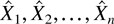
are mutually independent, with

.

Corollary 3.7: Let {X_k, k = 1,2,…} denote a sequence of mutually independent

-valued rvs. For each k = 1,2,…, let

denote an independent version of X_k. Assume the rvs

to be mutually independent. If

for all k = 1,2,…, then for each K = 1,2,…, the rv

is an independent version of

and

We also note the following convergence result [12, Thm.3.1, p.112].

Lemma 3.8: Let {X_n, n = 1,2,…} and {Y_n, n = 1,2,…} denote two sequences of

-valued rvs such that X_n ⇒_n X_∞ and Y_n ⇒_n Y_∞. If X_n ≤_sm Y_n for each n = 1,2,…, then X_∞ ≤_sm Y_∞.

Finally, we find it useful to extend some of the earlier definitions to sequences of rvs.

Definition 3.9: The two

-valued sequences X = {X_n, n = 1,2,…} and Y = {Y_n, n = 1,2,…} satisfy the relation X ≤_sm Y if (X₁,…,X_n) ≤_sm (Y₁,…,Y_n) for all n = 1,2,….

Definition 3.10: For sequences of

-valued rvs

, we say that

is an independent version of X if for each n = 1,2,…, the

-valued rv

is an independent version of the

-valued rv (X₁,…,X_n).

4. POSITIVE DEPENDENCE

Positive dependence in a collection of rvs can be captured in several ways. The association of rvs is one of the most useful such characterizations; it was introduced by Esary, Proschan, and Walkup [6] and has proved useful in various settings [2].

Definition 4.1: The

-valued rvs {X₁,…,X_n} are associated if, with X = (X₁,…,X_n), the inequality

holds for all nondecreasing functions

for which the expectations exist and are finite.

Here, we focus on a stronger notion of positive dependence:

Definition 4.2: The

-valued rvs {X₁,…,X_n} are stochastic increasingness in sequence (SIS) if for each k = 1,2,…,n − 1, the family of conditional distributions {[X_k+1|X₁ = x₁,…,X_k = x_k]} is stochastically increasing in x = (x₁,…,x_k) on the support of (X₁,…,X_k).

More precisely, this definition states that for each k = 1,2,…,n − 1, for x and y in

with x ≤ y componentwise on the support of (X₁,…,X_k), it holds that

where [X_k+1|(X₁,…,X_k) = x] denotes any rv distributed according to the conditional distribution of X_k+1 given (X₁,…,X_k) = x (with a similar interpretation for [X_k+1|(X₁,…,X_k) = y]).

These definitions can be extended to sequences in a natural way along the lines of Definition 3.9.

Definition 4.3: The

-valued sequence X = {X_n, n = 1,2,…} is SIS (resp. associated) if for each n = 1,2,…, the rvs {X₁,…,X_n} are SIS (resp. associated).

If the

-valued rvs {X₁,…,X_n} are SIS, then they are necessarily associated [2, Thm.4.7, p.146], but the converse might not be true. The next result was established by Meester and Shanthikumar [11] and relates the SIS property to the supermodular ordering. This fact will prove crucial for subsequent developments in this article.

Theorem 4.4: If the

-valued rvs {X₁,…,X_n} are SIS, then

where

is the independent version of (X₁,X₂,…,X_n).

5. MODELING ON–OFF SOURCES

A discrete-time on–off source with peak rate r is described by a succession of cycles, each such cycle comprising an off period followed by an on period. During the on periods, the source is active and produces “fluid” at a constant rate

. The activity of the source is then described by the {0,1}-valued process {A_t, t = 0,1,…} given by

for all t = 0,1,…, with the source active (resp. silent) during time slot [t,t + 1) if A_t = 1 (resp. A_t = 0).

An independent on–off source is one for which (1) the {1,2,…}-valued rvs {I_n, n = 1,2,…} and {B_n, n = 1,2,…} are mutually independent rvs which are independent of the pair of rvs I₀ and B₀ associated with the initial cycle and (2) the rvs {I_n, n = 1,2,…} (resp. {B_n, n = 1,2,…}) are independent and identically distributed (i.i.d.) rvs with generic off-period duration rv I (resp. on-period duration rv B). Throughout the generic rvs, I and B are assumed to be independent {1,2,…}-valued rvs such that 0 < E[I], E[B] < ∞. We simply refer to the independent on–off process just defined as the on–off source (I,B).

In general, the activity process (11) is not stationary unless the

-valued rvs I₀ and B₀ are selected appropriately. One possible way is to use the following variation on constructions given in [1,14]: With

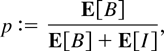
we introduce the {0,1}-valued rv U given by

Let I^{[starf ]} and B^{[starf ]} denote two {1,2,…}-valued rvs distributed according to the forward recurrence time (7) associated with I and B, respectively. A stationary version of (11), still denoted {A_t, t = 0,1,…}, is now obtained by selecting (I₀,B₀) so that

with rvs U, B, B^{[starf ]}, and I^{[starf ]} taken to be mutually independent and independent of the rvs {I_n,B_n, n = 1,2,…}. With this selection, the rvs {A_t, t = 0,1,…} form a stationary sequence with

where p is the average rate (12).

Note that the independent version of the stationary on–off process is a sequence

of i.i.d. {0,1}-valued rvs, with

where p is as above. It is easily seen that

is also a stationary on–off process with a geometric on period and off period; that is, the corresponding on-period duration rv B (resp. off-period duration rv I) is geometrically distributed with parameter p (resp. 1 − p)

For α (0 < α < 1), an {1,2…}-valued rv X is said to be a geometric rv with parameter α if it is distributed according to the pmf P[X = k] = α^k−1(1 − α) for all k = 1,2,…, in which case, we write

.

]. In other words,

can be interpreted as the discrete-time stationary on–off process

.

7. SUPERPOSITION OF FINITELY MANY SOURCES

Multiplexing is a major function in communication networks, with multiplexed traffic processes being created at routers and multiplexer buffers. Thus, with an on–off source representing a traffic stream, we construct multiplexed traffic by superposing a number of on–off sources. In this and the next section, we present results on the comparison (2) for the superposition of both a finite and an infinite number of independent on–off sources, respectively, the latter case giving rise to the so-called M|G|∞ input model.

More formally, consider K independent, but not necessarily identically distributed, on–off sources. For each k = 1,2,…,K, let {A_t^k,t = 0,1,…} denote the stationary on–off source (I^k,B^k). The superposition of these K on–off processes results in the stationary process {M_t^K,t = 0,1,…} given by

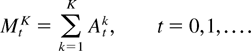
Its traffic intensity

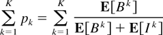
represents the average number of arrivals per slot generated by the superposition process.

Assume now that for each k = 1,2,…,K, the comparison

holds, where

is the independent version of {A_t^k,t = 0,1,…}. Proposition 6.1 provides sufficient conditions for (18) to hold.

By appealing to Corollary 3.7, it is a simple matter to conclude that

where the independent versions

, are taken to be mutually independent and

is the independent version of

.

8. SUPERPOSITION OF INFINITELY MANY SOURCES

We now consider the superposition of i.i.d. on–off sources as the number of sources grows unboundedly large. Some form of rescaling is needed in order to ensure a nontrivial limit. More precisely, for each K = 1,2,…, let the kth on–off source {A_t^(K,k) ,t = 0,1,…}, k = 1,…,K, be a stationary on–off source with same on-period and off-period duration rvs (I^(K),B). The resulting superposition process {M_t^K,t = 0,1,…} given in (16) becomes

with traffic intensity λ_KE[B], where

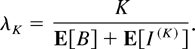
As K goes to infinity, Likhanov et al. [8] have shown that the limiting process of the superposition (20) is the stationary M|G|∞ input process, which counts the number of busy servers in the infinite server system fed by a discrete-time Poisson process with rate λ (customers/time slot) and with generic service time B (expressed in time slots).⁴

Theorem 8.1: Let {M_t^K,t = 0,1,…} be the superposition of K i.i.d. stationary on–off sources (I^(K),B). If lim_K→∞ λ_K = λ for some λ > 0 and lim_K→∞ P[I^(K) ≤ r] = 0 for each r = 1,2,…, then

where {M_t,t = 0,1,…} is the M|G|∞ process (λ,B).

Theorem 8.1 is essentially a discrete-time version of the celebrated Palm–Khintchin theorem, with the session durations playing the role of marks. The on-period duration rv B in the on–off processes simply mutates into the session duration rv in the M|G|∞ model. We note that this limiting process does not depend on the fine details of the off-period duration distributions.

As shown below, this last fact provides a natural vehicle for establishing a form of the comparison result (2) for M|G|∞ processes. Indeed, with Theorem 8.1 in mind, given a target M|G|∞ model (λ,B), we can construct a sequence of superposition processes (20) that converges in distribution to the M|G|∞ process (λ,B). However, as we have some latitude in selecting the rv I^(K), we will make a choice that guarantees the convergence (22) and yet ensures (19) for large K, say by satisfying the assumptions of Proposition 6.1 or 6.2 for the component processes. The desired conclusion would then follow from Lemma 3.8. This approach gives rise to the following comparison result:

Theorem 8.2: Let {M_t,t = 0,1,…} be an M|G|∞ input process (λ,B) such that B and B^{[starf ]} are DFR rvs. Its independent version

is a sequence of i.i.d. Poisson rvs with mean λE[B] and we have the comparison

Theorem 8.2 is not asserting the validity of the SIS property for M|G|∞ input processes, but rather a consequence of it. We were not able to prove this SIS property, and, in fact, we suspect that it does not hold true.

The proof of Theorem 8.2 given below relies on Theorem 8.1 and on the observations of Section 7. Another proof under no DFR assumption on the rvs B and B^{[starf ]} is provided in [21].

Proof: Fix K = 1,2,… such that K > λ(1 + E[B]) and consider the superposition process (20) where for each k = 1,…,K, the component process {A_t^(K,k) ,t = 0,1,…} is the on–off source (I^(K),B). We wish to select the rv I^(K) so that λ_K = λ, with (21) then yielding the relation

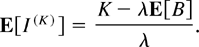
This can be achieved by taking

for some 0 < α(K) < 1, in which case, E[I^(K)] = α(K)⁻¹ and the mean value condition (24) implies

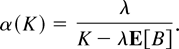
It is clear that lim_K→∞ α(K) = 0 and lim_K→∞ P[I^(K) ≤ r] = 0 for each r = 1,2,…. Consequently, the sequence of rvs {I^(K), K = 1,2,…} satisfies the requirements of Theorem 8.1, and (22) holds, with {M_t,t = 0,1,…} being the M|G|∞ input process (λ,B).

Next, we turn to the the SIS conditions of Proposition 6.2 for the component on–off processes defined earlier. For each K = 1,2,…, it is easy to check that I^(K) =_st I^{(K)[starf ]} and that these rvs are DFR since h_I^(K)(t) = α(K) for all t = 1,2,…. Thus, by taking the rvs B and B^{[starf ]} to be DFR, conditions (A.1) and (A.3) are satisfied. Conditions (A.2) and (A.4) require that

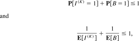
respectively. However, lim_K→∞ P[I^(K) = 1] = 0 and lim_K→∞ E[I^(K)] = ∞, from which conditions (A.2) and (A.4) are indeed satisfied if K is large enough, say K > K′ for some K′ > 0. Indeed, recall that E[B] ≥ 1 since B is {1,2,…}-valued.

Thus, whenever K > K′, the rvs I^(K) and B satisfy conditions (A.1)–(A.4), from which for each k = 1,…,K, the component process {A_t^(K,k) ,t = 0,1,…} is SIS, and by Theorem 4.4, we get

where

is the independent version of {A_t^(K,k) ,t = 0,1,…}.

As in Section 7, upon combining (25) and Corollary 3.7, we obtain

with

denoting the independent version of {M_t^K,t = 0,1,…}. We have

where the independent versions

, are taken to be mutually independent. The independent version

is a sequence of i.i.d. {0,1}-valued rvs with

for all t = 0,1,…, where

Consequently, for each t = 0,1,…, the rv

is a binomial rv with parameters (K,p(K)), from which the independent version

is a sequence of i.i.d. binomial rvs with parameters (K, λE[B]/K).

We are now ready to let K go to infinity in (26): By Lemma 3.8, we obtain the desired conclusion (23) if we show that

for some collection

of i.i.d. Poisson rvs with parameter λE[B]. Indeed, it is well known [13, Prop.2, p.277] that the stationary M|G|∞ input process (λ,B) has Poisson marginals with parameter λE[B], from which such a limit

would, indeed, be the independent version of the M|G|∞ input process {M_t,t = 0,1,…}. By Poisson's convergence theorem, for each t = 0,1,…, the binomial rv

with parameters (K, λE[B]/K) converges in distribution to a Poisson rv with mean λE[B], and the desired convergence (27) of the sequences of i.i.d. rvs readily follows. █

9. EXPRESSIONS FOR STATIONARY ON–OFF SOURCES

We begin the proof of Proposition 6.1 by developing some needed expressions. Indeed, for the stationary on–off source (I,B), the SIS condition takes a much simpler form, which we now present. For each t = 0,1,…, with the notation A^t = (A₀,…,A_t), we need to establish the inequalities

for any pair x^t = (x₀,…,x_t) and y^t = (y₀,…,y_t) in {0,1}^t+1 such that x^t ≤ y^t componentwise in {0,1}^t+1 with

As we proceed to evaluate the relevant conditional probabilities, in all cases we rely on the basic observation that

for every x^t in {0,1}^t+1 for which P[A^t = x^t] > 0. We first find expression (30) of the stationary on–off source for the case t = 0.

Lemma 9.1: For the stationary on–off source (I,B), we have

and

Proof: Conclusions (31) and (32) are easy consequences of the facts

since P[B ≥ 1] = 1, and

To describe the results when t = 1,2,…, we associate with any x^t in {0,1}^t+1 the index

of “last change” given by

If

, then

, whereas if

, then x₀ = x₁ = ··· = x_t. Fix t = 1,2,… throughout.

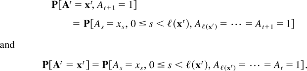
Proposition 9.2: For the stationary on–off source (I,B), for each x^t in {0,1}^t+1 with x_t = 1, we have

provided P[A^t = x^t] > 0.

Proof: With x_t = 1, we already note the relations

If

, then with some rv B independent of

, we conclude that

and

The first half of (33) follows readily by combining (34) and (35) through (30).

On the other hand, if

, then x^t = (1,…,1) and it holds that

and

The second half of (33) is obtained by combining (36) and (37) via (30). █

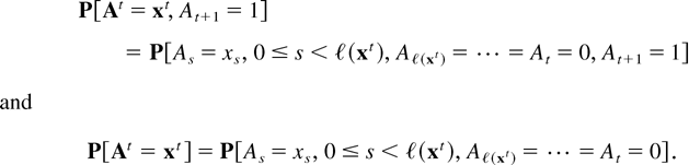
Proposition 9.3: For the stationary on–off source (I,B), for each x^t in {0,1}^t+1 with x_t = 0, we have

provided P[A^t = x^t] > 0.

Proof: The proof follows a pattern similar to that of Proposition 9.2. With x_t = 0, we obtain the relations

If

, then with some pair of independent rvs I and B which are independent of

, we conclude that

and

Combining (39) and (40) through (30), we get the first half of (38).

On the other hand, if

, then x^t = (0,…,0) and it holds that

and

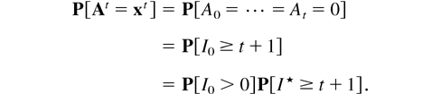
We conclude to the second half of (38) by combining (41) and (42) via (30). █

As a by-product of the proofs of Propositions 9.2 and 9.3, we note the following conditions for P[A^t = x^t] > 0 to hold: With x_t = 1, it follows from (35) and (37) that we need

. Similarly, with x_t = 0, we conclude from (40) and (42) that we need

.

10. A PROOF OF PROPOSITION 6.1

For each t = 0,1,…, we need to show that (28) holds for any pair of distinct elements x^t and y^t in {0,1}^t+1 with x^t ≤ y^t componentwise such that (29) holds.

For t = 0, (29) automatically holds here since P[A₀ = 1] = 1 − P[A₀ = 0] = p with 0 < p < 1. By Lemma 9.1, we see that (28) reduces to

which is equivalent to condition (iv).

For t = 1,2,…, three cases present themselves, depending on whether (a) x_t = y_t = 1, (b) x_t = y_t = 0, and (c) x_t = 0 < y_t = 1. Recall that we are only interested in the situations where (29) is satisfied. We consider each one of three cases in turn.

Case (a): With x_t = y_t = 1, the condition x^t ≤ y^t implies

. If

, then

as well. By Proposition 9.2, (28) reduces to

with

. Inequality (44) does hold when B is DFR. If

, then

(for otherwise, x^t = y^t) and Proposition 9.2 this time shows that (28) is equivalent to

with both

. The validity of this last inequality is an easy consequence of Lemma 2.2 and of the fact that both B and B^{[starf ]} are DFR rvs since on the considered range, we have

Case (b): With x_t = y_t = 0, the condition x^t ≤ y^t now implies

. If

, then

, and by Proposition 9.3, the desired inequality (28) reduces to

with

. Inequality (45) is implied by the fact that the rv I is DFR under condition (i). If

, then

(for otherwise, x^t = y^t) and Proposition 9.3 shows that the desired inequality (28) is equivalent to

with both

. As earlier, this is the case on the specified range by virtue of Lemma 2.2, which yields

since I and I^{[starf ]} are DFR rvs.

Case (c): With x_t = 0 < y_t = 1, four possible scenarios need to be considered when invoking Propositions 9.2 and 9.3 to rewrite (28) in reduced form. First, if

, then (28) can be rewritten as

with t + 1 in both

, and this inequality does hold by virtue of conditions (iii) and (iv) (or, equivalently, (43)).

Next, if

, then (28) becomes

with

. Because I^{[starf ]} and B are DFR, we get

and (47) indeed holds by virtue of condition (v). Symmetrically, if

, then (28) reads

with

. Now, the fact that B^{[starf ]} and I are DFR leads to

and (48) is now immediate from condition (v).

Finally, if

, then (28) is equivalent to

with

. If

, then

while

, and (49) is now a simple consequence of condition (ii) since the rvs I and B are DFR. A symmetric argument holds mutatis mutandis if

. We complete the proof by noting that the case

is not possible under the constraints x_t = 0, y_t = 1, and x^t ≤ y^t componentwise.

11. RENEWAL ON–OFF SOURCES

In the definition of on–off processes, the initial pair (I₀,B₀) could have been selected so that

with I and B independent. The resulting on–off source is said to be the renewal (version of the) on–off source (I,B). Its independent version

is simply a collection of mutually independent {0,1}-valued rvs with

and, in general, can no longer be interpreted as an on–off process, be it stationary or renewal.

We now present conditions for the renewal on–off source (I,B) to be SIS. The analog of Proposition 6.1 is given next.

Proposition 11.1: The renewal on–off source (I,B) satisfies the SIS property whenever conditions (i)–(ii) of Proposition 6.1 hold.

Here, the analog of Proposition 6.2 takes the following form:

Proposition 11.2: Conditions (i)–(ii) in Proposition 6.1 are implied by conditions (A.1)–(A.2) of Proposition 6.2.

Proposition 11.2 is established in a manner similar to that of Proposition 6.2, and we, therefore, omit the proof. As we now turn to the proof of Proposition 11.1, we first obtain (30) for the renewal on–off source (I,B) and then derive the corresponding SIS conditions. Here, we have I₀ =_st I so that P[A₀ = 0] = 1. This observation leads to the following analog of Lemma 9.1.

Lemma 11.3: For the renewal on–off source (I,B), we have

Proof: As in the proof of Lemma 9.1, conclusion (51) is an easy consequence of the facts

by the independence of the rvs I₀ and B₀ and the fact that P[B₀ ≥ 1] = 1. █

In the renewal case, the analogs of Propositions 9.2 and 9.3 can be expressed more compactly, as the next proposition shows.

Proposition 11.4: Fix t = 1,2,…. For the renewal on–off source (I,B), for each x^t in {0,1}^t+1 with P[A^t = x^t] > 0, we have the following. If x_t = 1, then

and if x_t = 0, then

Proof: We need not consider the case

with x_t = 1, for then x^t = (1,…,1), and the event [A^t = x^t] cannot occur because I₀ =_st I implies A₀ =_st 0.

A careful inspection of the proofs of Propositions 9.2 and 9.3 shows that both (52) and (53) hold when

. Hence, only the case

with x_t = 0 needs to be considered in order to complete the proof of (53). In that case, we have x^t = (0,…,0), from which (41) and (42) now become

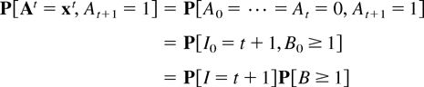
and

We reach the desired result by combining (54) and (55) via (30). █

A proof of Proposition 11.1 can now be given. For each t = 0,1,…, we need to show that (28) holds for distinct elements x^t and y^t in {0,1}^t+1 satisfying (29) and such that x^t ≤ y^t componentwise.

For t = 0, x₀ = 0 and y₀ = 1, so that there is no need for comparison here because P[A₀ = y₀] = 0.

Fix t = 1,2,…. As in the proof of Proposition 6.1, three cases present themselves, depending on whether (a) x_t = y_t = 1, (b) x_t = y_t = 0, and (c) x_t = 0 < y_t = 1.

Case (a): With x_t = y_t = 1, the condition x^t ≤ y^t implies

. By Proposition 11.4, (28) can be rewritten as

with

. It is clear that (56) holds because B is assumed DFR.

Case (b): With x_t = y_t = 0, the condition x^t ≤ y^t implies

. By Proposition 11.4, (28) reduces to

with

, and the validity of (57) is implied by the fact that the rv I is DFR.

Case (c): With x_t = 0 < y_t = 1 and invoking Proposition 11.4, we can rewrite (28) in reduced form as

with

. As in the proof of Proposition 6.1, we must have

both hold. Hence, it is a simple matter to check that in all feasible situations either

. The validity of (58) is then guaranteed under condition (ii) because the rvs I and B are DFR rvs.