

1. Introduction
Suspensions of particles in a bulk fluid commonly occur in nature and in several engineering applications. Einstein (Reference Einstein1906) was the first to quantitatively determine the viscosity of a dilute suspension of spherical particles. More specifically, the presence of the particles leads to an increase in the energy dissipation inside the fluid which is effectively related to an increase in viscosity. The basis of these calculations was to compute the rate of viscous dissipation in a large control volume concentric with a particle. Another milestone in suspension rheology is the work of Batchelor (Reference Batchelor1970). By employing volume averaging of the stresses inside the suspension, he found an elegant way of calculating the effective suspension properties, which in its most general form applies to arbitrary particle concentrations and shapes. His analytical solutions, however, are limited to dilute suspensions where only a single particle or the interaction of two particles is taken into account. Batchelor & Green (Reference Batchelor and Green1972) managed to go beyond that limit and computed the viscosity of suspensions up to second order in the volume concentration. Due to the hydrodynamic interactions of sufficiently small particles at higher concentrations, Brownian motion has to be taken into account and can be represented as a stochastic force (Batchelor Reference Batchelor1976, Reference Batchelor1977). However, in most of the work reported in the literature, higher-order approximations (in the concentration) are typically achieved through numerical simulations (Foss & Brady Reference Foss and Brady2000; Sierou & Brady Reference Sierou and Brady2001).
Whenever particles are attached to fluid interfaces, i.e. interfaces between a gas and a liquid or between two immiscible liquids, additional physical effects, such as capillarity, superpose to the effects present in the bulk of a fluid. In the past decades, systems with particles attached to fluid interfaces have been studied quite intensely, since the particles bring along unique properties not found for bare interfaces. Interfacial particles mechanically stabilize droplets (e.g. Binks Reference Binks2002; Aveyard, Binks & Clint Reference Aveyard, Binks and Clint2003; Dickinson Reference Dickinson2010; Wu & Ma Reference Wu and Ma2016; De Corato & Garbin Reference De Corato and Garbin2018). These composite structures are often referred to as liquid marbles (Aussillous & Quéré Reference Aussillous and Quéré2001). The evaporation rate of liquid marbles on surfaces is lower than that of bare droplets, since no liquid is in direct contact with the substrate (McHale & Newton Reference McHale and Newton2011). Liquid marbles enable the creation of hollow granules (Eshtiaghi, Liu & Hapgood Reference Eshtiaghi, Liu and Hapgood2010), are usually more mobile on surfaces than bare droplets, and can be positioned and transported via gravity (more precisely than a bare droplet since contact angle hysteresis is negligible) (Aussillous & Quéré Reference Aussillous and Quéré2001), as well as via applied magnetic (Bormashenko et al. Reference Bormashenko, Pogreb, Bormashenko, Musin and Stein2008) or electric fields (Newton et al. Reference Newton, Herbertson, Elliott, Shirtcliffe and McHale2007). Owing to these properties, potential applications are abundant. Liquid marbles may be used in the pharmaceutical, medical, chemical and cosmetic industries (Avramescu et al. Reference Avramescu, Ghica, Dinu-Pîrvu, Udeanu and Popa2018). Apart from that, particles attached to fluid interfaces play a role in creating nanostructured materials based on the Langmuir and Langmuir–Blodgett techniques (Park & Advincula Reference Park and Advincula2011) or in the stabilization of emulsions (Wu & Ma Reference Wu and Ma2016).
Potentially inspired by the manifold applications of interfacial particles, Lishchuk & Halliday (Reference Lishchuk and Halliday2009) were the first to calculate the effective dilatational and shear viscosities of a particle-laden interface in the dilute limit (surface concentration  $\phi _L \ll 1$) for particles having a contact angle of
 $\alpha = 90^{\circ }$. They used a method similar to that of Einstein (Reference Einstein1906). They further verified their results with lattice Boltzmann simulations and demonstrated good agreement if
 $\phi _L \le 0.15$. Later on, Lishchuk (Reference Lishchuk2014) modelled the effective dilatational viscosity of an interface densely decorated with particles, where Brownian motion was neglected and the contact angle was fixed to
 $\alpha = 90^{\circ }$. By employing a toroidal coordinate system, Lishchuk (Reference Lishchuk2016) calculated the effective dilatational surface viscosity in the dilute limit as a function of the contact angle
 $\alpha$, when both phases have a large viscosity contrast. The resulting integral had to be solved numerically.
What has not been achieved up to now is the determination of closed-form analytical expressions for the dilatational and shear viscosities of a particle-laden interface, valid for a broad range of contact angles  $\alpha$. Even though a semi-analytical solution for the effective dilatational viscosity has already been reported, the dependence of the interfacial shear viscosity on the contact angle of the particles has remained obscure, limiting the practical use of prior studies significantly. The main objective of the present work is to close the gap previous studies have left and shed more light on the rheology of interfacial suspensions. In § 2, we describe the problem, the model assumptions and the governing equations together with the boundary conditions. The stress-averaging method from Batchelor (Reference Batchelor1970) is applied on interfacial suspensions. In § 3, we make use of this method to calculate the effective surface viscosities up to second order in
 $\beta = \cos (\alpha )$, which are further discussed in § 4. Finally, in § 5 we summarize the main results of our work and indicate possible further studies.
2. Problem formulation and model assumptions
We consider a particle-laden fluid interface, consisting of identical spherical particles having a radius  $a$ and a contact angle
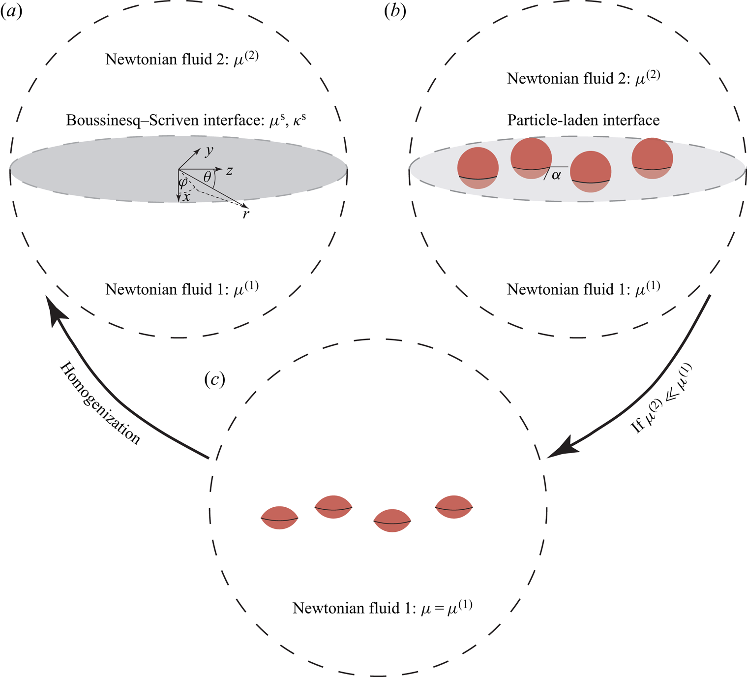
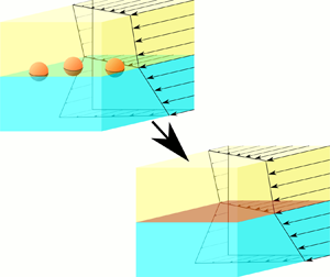
 $\alpha$. In the absence of particles, the infinitesimally thin interface (a so-called dividing surface or Gibbs interface (Slattery, Sagis & Oh Reference Slattery, Sagis and Oh2007)) separating the two phases is assumed to be ideal (massless/incompressible with vanishing surface stresses (Wang & Oberlack Reference Wang and Oberlack2011)). Ideal interfaces are commonly assumed in the absence of surfactants or impurities (e.g. Brenner Reference Brenner1991). We always consider an ideal interface and aim at computing the interfacial viscosities arising when we add particles. We do this in the framework of a homogenization method. That is, the particle-laden interface is represented by a homogeneous interface having effective viscosities (figure 1a,b).
Visualization of the similarities used for the computation of the effective surface viscosities represented by a Boussinesq–Scriven constitutive law (a); see (2.11). The basis of the calculation is spherical particles attached to an ideal interface (massless and vanishing stresses), which is equivalent to mirror-fused particles suspended in an infinite bulk fluid if the viscosity ratio  $\mu _2 / \mu _1$ vanishes asymptotically.

In general, hydrodynamic interparticle interactions, Brownian motion and long-range capillary interactions (due to a deformation of the fluid interface) bring along many complications that leave us with a very complex problem that is usually inaccessible to analytical methods. To keep the problem tractable, the following assumptions are made:
(i) Both fluid phases are Newtonian and incompressible.
(ii) The Reynolds number in phase
 $1$ is small, i.e. $Re^{(1)} \ll 1$.
(iii) The radius of curvature of the fluid interface separating the two phases is much larger than the characteristic size
$a$ of the particles, and the capillary number $Ca$ is sufficiently small.(iv) The viscosity ratio between the two phases vanishes asymptotically, i.e.
$\mu ^{(2)}/ \mu ^{(1)}\to 0$.(v) The interfacial particles are neutrally buoyant, rigid, of spherical shape with radius
$a$, while the fluid interface assumes a contact angle of $\alpha$ on the particle surface.(vi) The interfacial suspension is dilute.
(vii) Brownian motion is negligible.
(viii) The total force and torque acting on each particle vanish.


Assumption (ii) simplifies the momentum balance by neglecting any transient and convective terms. For small capillary numbers  $Ca = \mu \mathcal {E} a/\gamma$, with
 $\mathcal {E} = \sqrt {\boldsymbol{\mathsf{E}}\,\textbf{:}\,\boldsymbol{\mathsf{E}}}$, the stress-jump balance can be expanded into a perturbation series in
 $Ca$. Here,
 $\gamma$,
 $\mathcal {E}$ and
 $\boldsymbol{\mathsf{E}}$ denote the interfacial tension between phases 1 and 2, a characteristic shear or dilatational rate and the rate-of-strain tensor, while : defines the double contraction product. As long as the radius of curvature of the interface is much larger than the characteristic size of a particle (assumption (iii)), the curvature of the interface can asymptotically be neglected in the zeroth order in
 $Ca$. Small capillary numbers induce dominating surface tension forces compared to viscous forces. Assumption (iv) is a reasonable approximation for any gas–liquid system, since, taking the air–water system as an example, we obtain
 $\mu ^{air} / \mu ^{water} \approx 0.02$ (Petkov et al. Reference Petkov, Denkov, Danov, Velev, Aust and Durst1995). When it is assumed that the spherical particles are neutrally buoyant and rigid, the fluid interface remains flat even if particles are attached to it (assumption (v)). Generally, fluid interfaces are free of shear stresses (if no Marangoni stresses are present); therefore, from this together with assumption (iii), the interface has all the properties of a symmetry plane. Consequently, the velocity and pressure field around the particles can be calculated by replacing the interfacial particles with particles consisting of two fused mirror-reflected spherical caps in an unbounded fluid, as shown in figure 1(b,c). This kind of symmetry argument has already been used in the calculation of the drag force acting on an interfacial particle driven by an applied force (Dörr & Hardt Reference Dörr and Hardt2015; Dörr et al. Reference Dörr, Hardt, Masoud and Stone2016), in the calculation of the electrophoretic mobility of an interfacial particle (Eigenbrod, Bihler & Hardt Reference Eigenbrod, Bihler and Hardt2018) and in the semi-analytical calculation of the effective dilatational viscosity of particle-laden interfaces (Lishchuk Reference Lishchuk2016). Therefore, the upper phase (phase 2) does not affect the interfacial particles. The effective interfacial properties are thus solely determined by the stresses acting in fluid phase 1. From now on, all material properties appearing in the equations correspond to phase 1 and we suppress the superscripts.
Interfacial particles may interact through different mechanisms, e.g. through hydrodynamic interactions due to the mean relative velocity of the particles or through velocity fluctuations due to Brownian motion. Furthermore, it has been shown that when interfacial particles execute an oscillating motion normal to the interface (Toro-Mendoza, Rodriguez-Lopez & Paredes-Altuve Reference Toro-Mendoza, Rodriguez-Lopez and Paredes-Altuve2017), the resulting capillary waves induce an interaction. A particle–particle interaction is also induced by the dynamic interfacial deformation of particles moving along a fluid interface (Dörr & Hardt Reference Dörr and Hardt2015). Even in the static case the deformation of the interface leads to capillary interactions between particles (Léandri & Würger Reference Léandri and Würger2013; Galatola & Fournier Reference Galatola and Fournier2014). Naturally, all of these interactions decay with the interparticle distance. In a similar way as in the calculation of the effective viscosity of a bulk suspension we need to assume that the interparticle distance is large enough to render these interactions negligible (assumption (vi)). Therefore, among other things, it is assumed that the perturbation velocity field due to the presence of a particle does not influence neighbouring particles. It should be noted that Batchelor (Reference Batchelor1977) has shown that the dilute-limit solution by Einstein (Reference Einstein1906) holds even in the presence of Brownian motion. However, this general statement cannot be made in the case of interfacial particles, due to the capillary waves mentioned above. When no external force or torque is applied to the suspension (e.g. through an external electric or magnetic field) and inertial effects are neglected, the particles follow the flow in such a way that the hydrodynamic force and torque on each particle vanish (assumption (viii)).
Before we turn to the discussion of the governing equations as well as the corresponding boundary conditions, we comment on the definition of the surface concentration by Lishchuk & Halliday (Reference Lishchuk and Halliday2009), i.e.
 \begin{equation} \phi_L = \frac{N {\rm \pi}a^2}{A}. \end{equation}
Here  $A$ is the total area of the fluid interface,
 $N$ the number of particles attached to the interface and
 $a$ the radius of the particles. For contact angles deviating from
 $\alpha = 90^{\circ }$, however, the fraction of the area of the fluid interface cutting through the particles is smaller than this, and is given by
 \begin{equation} \phi = \frac{N {\rm \pi}a^2 [1-\cos^2(\alpha)]}{A}. \end{equation}
We later compare the semi-analytical results by Lishchuk (Reference Lishchuk2016) to our theoretical results and therefore have to keep both definitions in mind. Apart from that, we do not use the definition from (2.1).
2.1. Governing equations and boundary conditions
As already pointed out when discussing the underlying assumptions, particles at ideal interfaces can be represented by mirror-fused particles in a bulk fluid; see figure 1(b,c). We therefore describe the governing equations and the corresponding boundary conditions referring to figure 1(c).
Following assumptions (i) & (ii), the governing equations are the Stokes equations, reading
 \begin{equation} \boldsymbol{\nabla} p_{tot} = \mu \nabla^2 \boldsymbol{u}_{tot}, \quad \boldsymbol{\nabla} \boldsymbol{\cdot} \boldsymbol{u}_{tot} = 0, \end{equation}
in which  $p_{tot}$ is the thermodynamic pressure,
 $\boldsymbol {u}_{tot}$ the velocity field and
 $\mu$ the dynamic viscosity (referring to phase 1). Here,
 $\boldsymbol {u}_{tot} = \boldsymbol {u}^{\infty } + \boldsymbol {u}$ is the superposition of an applied velocity field
 $\boldsymbol {u}^{\infty }$ and a disturbance velocity field
 $\boldsymbol {u}$ occurring through the presence of particles. The first equation in (2.3a,b) is the linearized momentum balance equation, in which the inertia terms as well as body force terms are neglected (assumption (v)). The second equation in (2.3a,b) ensures incompressibility in the bulk.
Next we consider an arbitrary applied velocity around the particles and linearize it around the origin of the coordinate system (shown in figure 1a), leading to the following (Brenner Reference Brenner1991):
 \begin{equation} \boldsymbol{u}^{\infty}(\boldsymbol{r}) \approx \boldsymbol{U}^{\infty} + \boldsymbol{\varOmega}^{\infty} \times \boldsymbol{r} + \boldsymbol{\mathsf{E}} \boldsymbol{\cdot} \boldsymbol{r}, \end{equation}
in which  $\boldsymbol {r}$ is the position vector and
 $|\boldsymbol {r}| = r$ its length. Generally, a particle suspended in the bulk can execute a translation and rotation due to the applied velocity field
 $\boldsymbol {u}^{\infty }(\boldsymbol {r})$ and, if the suspension is not dilute, to perturbations of the velocity field originating from nearby particles. The latter is ignored owing to assumption (vi). Consequently, the far field boundary condition for every particle is of the same mathematical form. In the following, we represent all of these non-interacting particles by a single particle to which this boundary condition applies, located at the centre of the coordinate system. The Stokes equations are linear, and consequently the boundary conditions at the surface of the representative particle as well as far away from the particle can be written as the difference between the translational and rotational velocity of the particle and the unperturbed applied, linearized velocity field. This yields
 \begin{equation} \left. \boldsymbol{u}\right|_{r_{\mathcal{P}}} = \boldsymbol{U}^{eff} + \boldsymbol{\omega}^{eff} \times \frac{\boldsymbol{r}}{r} r_{\mathcal{P}} - \boldsymbol{\mathsf{E}} \boldsymbol{\cdot} \frac{\boldsymbol{r}}{r} r_{\mathcal{P}}, \quad \mathrm{and}\quad \lim_{r \to \infty} \boldsymbol{u} = \boldsymbol{0}, \end{equation}
in which  $\boldsymbol {U}^{eff} = \boldsymbol {U} - \boldsymbol {U}^{\infty }$ is the effective translational velocity, defined as the difference between the velocity of each particle and the applied translational velocity;
 $\boldsymbol {\omega }^{eff} = \boldsymbol {\omega } - \boldsymbol {\varOmega }^{\infty }$ is the effective angular velocity; and
 $r_{\mathcal {P}}$ is the parametrization of the surface of the particle. The effective translational/rotational velocity is typically obtained through a force/torque balance at the particle. For spheres (
 $r_{\mathcal {P}} = a$) in an unbounded medium, it follows by Faxén's law (Happel & Brenner Reference Happel and Brenner2012; Kim & Karrila Reference Kim and Karrila2013) and in the absence of external forces or torques (assumption (viii)) that
 $\boldsymbol {U}^{eff} = \boldsymbol {0}$ and
 $\boldsymbol {\omega }^{eff} = \boldsymbol {0}$, leading to the boundary condition
 $\boldsymbol {u}|_{a} = - \boldsymbol{\mathsf{E}} \boldsymbol {\cdot } ({\boldsymbol {r}}/{r}) a$ at the surface of the particle. Translated to an interfacial particle, this corresponds to a particle having a contact angle of
 $\alpha = 90^{\circ }$. For non-spherical particles an effective translation and rotation might exist, which would affect the boundary conditions at the surface of the representative particle and consequently the effective viscosities. However, in appendix A we show that the effective translational and rotational velocities do not need to be considered in the present study. Consequently, the boundary conditions at the surface of the particle correspond to a pure straining flow field.
At this point, we have to restrict the rate-of-strain tensor  $\boldsymbol{\mathsf{E}}$, since in the absence of Marangoni stresses fluid interfaces are shear-free, and further, the flow is assumed to be incompressible. The rate-of-strain tensor then reads
 \begin{equation} \boldsymbol{\mathsf{E}} = \left[\begin{matrix} -\boldsymbol{\nabla}^{\mathcal{S}} \boldsymbol{\cdot} \boldsymbol{u}^{\mathcal{S}} & 0 & 0 \\ 0 & {\mathsf{E}}_{yy}^{\mathcal{S}} & {\mathsf{E}}_{yz}^{\mathcal{S}}\\ 0 & {\mathsf{E}}_{yz}^{\mathcal{S}} & {\mathsf{E}}_{zz}^{\mathcal{S}} \end{matrix} \right], \quad \boldsymbol{\mathsf{E}}^{\mathcal{S}} = \left[ \begin{matrix} {\mathsf{E}}_{yy}^{\mathcal{S}} & {\mathsf{E}}_{yz}^{\mathcal{S}}\\ {\mathsf{E}}_{yz}^{\mathcal{S}} & {\mathsf{E}}_{zz}^{\mathcal{S}}, \end{matrix} \right] \end{equation}
with  $\boldsymbol {\nabla }^{\mathcal {S}} \boldsymbol {\cdot } \boldsymbol {u}^{\mathcal {S}} = {\mathsf{E}}_{yy}^{\mathcal {S}} + {\mathsf{E}}_{zz}^{\mathcal {S}}$. The boundary conditions for a mirror-fused bulk particle can therefore be written as
 \begin{equation} \left. \boldsymbol{u}\right|_{r_{\mathcal{P}}} = - \boldsymbol{\mathsf{E}} \boldsymbol{\cdot} \frac{\boldsymbol{r}}{r} r_{\mathcal{P}}, \quad \mathrm{and}\quad \lim_{r \to \infty} \boldsymbol{u} = \boldsymbol{0}. \end{equation}
It is worth mentioning that (2.7a,b) describes a fixed particle with a no-slip condition on its surface in pure straining flow. In summary, (2.3a,b) and (2.7a,b) provide all necessary information to compute the flow around a mirror-fused particle in an unbounded fluid. Before we present a solution strategy, we introduce the underlying method employed for the computation of the effective interfacial viscosities. More details of the derivation leading to the following relationship are given in appendix B. We obtained
 \begin{gather} \langle \boldsymbol{\sigma}^{\mathcal{S}} \rangle \,\textbf{:}\,\boldsymbol{\mathsf{E}}^{\mathcal{S}} = \frac{N}{2 A} \boldsymbol{\mathsf{S}} \,\textbf{:}\,\boldsymbol{\mathsf{E}}, \end{gather}
 \begin{gather} \boldsymbol{\mathsf{S}} = \int_{A_{\mathcal{P}}} \tfrac{1}{2} (\boldsymbol{r} \boldsymbol{\varPi} \boldsymbol{\cdot} \boldsymbol{n} + \boldsymbol{\varPi} \boldsymbol{r} \boldsymbol{\cdot} \boldsymbol{n})-\tfrac{1}{3} \boldsymbol{r} \boldsymbol{\cdot} \boldsymbol{\varPi} \boldsymbol{\cdot} \boldsymbol{n}\ \boldsymbol{\mathsf{I}} - \mu(\boldsymbol{n} \boldsymbol{u} + \boldsymbol{u} \boldsymbol{n}) \,\mathrm{d}A. \end{gather}
Here,  $\langle \boldsymbol {\sigma }^{\mathcal {S}}\rangle$,
 $\boldsymbol {\varPi }$ and
 $A_{\mathcal {P}}$ are the area-averaged deviatoric interfacial stresses, the total bulk stress and the surface of a mirror-reflected particle suspended in the bulk of the fluid carrying the asymptotically dominating viscosity;
 $\boldsymbol{\mathsf{S}}$ is the stresslet. Making use of (2.2), the interfacial suspension stress reads
 \begin{equation} \langle \boldsymbol{\sigma}^{\mathcal{S}} \rangle \,\textbf{:}\,\boldsymbol{\mathsf{E}}^{\mathcal{S}} = \frac{\phi}{2 {\rm \pi}a^2 [1 - \cos^2(\alpha)]} \boldsymbol{\mathsf{S}} \,\textbf{:}\,\boldsymbol{\mathsf{E}}. \end{equation}
The foregoing derivation is still very general, since we have not specified a constitutive equation for the interfacial stresses. We may consider a compressible Newtonian interface, which is described by a Boussinesq–Scriven law (Boussinesq Reference Boussinesq1913; Scriven Reference Scriven1960):
 \begin{equation} \boldsymbol{\sigma}^{\mathcal{S}} = (\kappa^{\mathcal{S}} - \mu^{\mathcal{S}}) (\boldsymbol{\nabla}^{\mathcal{S}} \boldsymbol{\cdot} \boldsymbol{u}^{\mathcal{S}} ) \boldsymbol{\mathsf{I}}^{\mathcal{S}} + 2 \mu^{\mathcal{S}} \boldsymbol{\mathsf{E}}^{\mathcal{S}}, \end{equation}
where  $\kappa ^{\mathcal {S}}$,
 $\mu ^{\mathcal {S}}$ and
 $\boldsymbol{\mathsf{I}}^{\mathcal {S}}$ are the surface dilatational viscosity, the surface shear viscosity and the surface identity tensor, respectively. As for the constitutive law of a Newtonian fluid in the bulk, it can be shown with the help of the second law of thermodynamics that
 $\kappa ^{\mathcal {S}} \geq 0$ and
 $\mu ^{\mathcal {S}} \geq 0$ (Gatignol & Prud'homme Reference Gatignol and Prud'homme2001). Furthermore, experimentalists have shown that usually
 $\kappa ^{\mathcal {S}} > \mu ^{\mathcal {S}}$ in the case of particle-free interfaces (e.g. Fox & Rock Reference Fox and Rock1946; Maru & Wasan Reference Maru and Wasan1979). Based on the Boussinesq–Scriven law, we write
 \begin{equation} \langle\boldsymbol{\sigma}^{\mathcal{S}}\rangle \,\textbf{:}\,\boldsymbol{\mathsf{E}}^{\mathcal{S}} = (\kappa^{\mathcal{S}} - \mu^{\mathcal{S}}) (\langle \boldsymbol{\nabla}^{\mathcal{S}} \boldsymbol{\cdot} \boldsymbol{u}^{\mathcal{S}} \rangle)^2 + 2 \mu^{\mathcal{S}} (\langle \boldsymbol{\mathsf{E}}^{\mathcal{S}} \rangle)^2, \end{equation}
where we have used the shorthand notation  $(\langle \boldsymbol{\mathsf{E}}^{\mathcal {S}} \rangle )^2 = \langle \boldsymbol{\mathsf{E}}^{\mathcal {S}} \rangle \,\textbf{:}\,\langle \boldsymbol{\mathsf{E}}^{\mathcal {S}} \rangle$.
3. Effective surface viscosities of a particle-laden interface in the dilute limit
In this section, we present the strategy applied for the calculation of the effective surface viscosities corresponding to a Boussinesq–Scriven interface with the help of (2.10) and (2.12). The solution procedure of (2.3a,b) subject to the boundary conditions from (2.7a,b) is discussed in more detail in appendix B. In general, our solution strategy is based on a domain perturbation method. More specifically, we consider the solution of the Stokes equations for a slightly deformed sphere in pure straining flow. To keep the calculation manageable, we limit ourselves to the second-order perturbation in a small parameter  $\beta$.
According to Brenner (Reference Brenner1964), the parametrization of the surface of a slightly deformed sphere can be written as
 \begin{equation} r_{\mathcal{P}} \approx a + a \beta f(\theta,\varphi) + a \beta^2 g(\theta, \varphi), \end{equation}
in which  $a$ is the radius of the undeformed sphere,
 $\beta$ is a perturbation parameter, and
 $f(\theta ,\varphi )$ and
 $g(\theta ,\varphi )$ are two functions of the azimuthal and the polar angle. For a mirror-fused particle consisting of two spherical caps,
 $\beta = \cos (\alpha )$ is a useful choice (Dörr & Hardt Reference Dörr and Hardt2015; Dörr et al. Reference Dörr, Hardt, Masoud and Stone2016; Eigenbrod et al. Reference Eigenbrod, Bihler and Hardt2018), and we obtain
 \begin{equation} r_{\mathcal{P}} \approx a + a \beta \sin(\theta) |\cos(\varphi)| + a \beta^2 ~\frac{\sin^2(\theta) \cos^2(\varphi) - 1}{2}, \end{equation}
from which  $f(\theta ,\varphi ) = \sin (\theta ) |\cos (\varphi )|$ and
 $g(\theta , \varphi ) = ({\sin ^2(\theta ) \cos ^2(\varphi ) - 1})/{2}$ can be read off. With (3.2) and (2.7a,b), the boundary condition can be rewritten. Following the procedure first presented by Brenner (Reference Brenner1964), the velocity and pressure field are expanded into a perturbation series in
 $\beta$ (in which the Stokes equations have to be fulfilled at each order) and each contribution of given order in
 $\beta$ is Taylor-expanded in
 $r$ around (
 $r-a$). After some rearrangement, the following boundary conditions are obtained:
 \begin{gather} \left. \boldsymbol{u}^{(0)} \right|_a = - \boldsymbol{\mathsf{E}} \boldsymbol{\cdot} \frac{\boldsymbol{r}}{r} a, \end{gather}
 \begin{gather} \left. \boldsymbol{u}^{(1)} \right|_a = - a f(\theta, \varphi) \left( \boldsymbol{\mathsf{E}} \boldsymbol{\cdot} \frac{\boldsymbol{r}}{r} + \left. \frac{\partial \boldsymbol{u}^{(0)}}{\partial r}\right|_a \right), \end{gather}
 \begin{align} \left. \boldsymbol{u}^{(2)} \right|_a &= - a f(\theta, \varphi) \left. \frac{\partial \boldsymbol{u}^{(1)}}{\partial r}\right|_a - a g(\theta, \varphi) \left(\boldsymbol{\mathsf{E}} \boldsymbol{\cdot} \frac{\boldsymbol{r}}{r} + \left. \frac{\partial \boldsymbol{u}^{(0)}}{\partial r} \right|_a \right) \nonumber\\ &\quad - \frac{a^2}{2} f(\theta,\varphi)^2 \left. \frac{\partial^2 \boldsymbol{u}^{(0)}}{\partial r^2}\right|_a . \end{align}
Here, the superscript corresponds to the approximation order in  $\beta$. It should be noted that the boundary conditions on the slightly deformed sphere are mapped onto an undeformed sphere. Clearly, the solution of the Stokes equations satisfying the boundary condition (3.3) corresponds to an undeformed sphere in pure straining and is readily known. The boundary condition of the first-order solution is uniquely determined by the zeroth-order solution. To proceed, both functions
 $f(\theta , \varphi )$ and
 $g(\theta , \varphi )$ are expanded in surface spherical harmonics (Brenner Reference Brenner1964). For the first-order solution, we therefore expand
 $f(\theta , \varphi ) = \sin (\theta ) |\cos (\varphi )| = \sum _{k = 0}^{\infty } f_k$, using a method described in Byerly (Reference Byerly1893) or MacRobert (Reference MacRobert1947). The terms of this infinite sequence are given through
 \begin{gather} A_{0,k} = \frac{2k+1}{4{\rm \pi}} \int_{0}^{2{\rm \pi}} \int_{0}^{\rm \pi} f(\theta,\varphi) P_k(\cos(\theta)) \sin(\theta)\,\mathrm{d} \theta\,\mathrm{d} \varphi, \end{gather}
 \begin{gather} A_{n,k} = \frac{2k+1}{2{\rm \pi}} \frac{(k-n)!}{(k+n)!} \int_{0}^{2{\rm \pi}} \int_{0}^{\rm \pi} f(\theta,\varphi) \cos(n \varphi) P_k^n(\cos(\theta)) \sin(\theta)\,\mathrm{d} \theta\,\mathrm{d} \varphi, \end{gather}
 \begin{gather} B_{n,k} = \frac{2k+1}{2{\rm \pi}} \frac{(k-n)!}{(k+n)!} \int_{0}^{2{\rm \pi}} \int_{0}^{\rm \pi} f(\theta,\varphi) \sin(n \varphi) P_k^n(\cos(\theta)) \sin(\theta)\,\mathrm{d} \theta\,\mathrm{d} \varphi, \end{gather}
 \begin{gather} f_k = A_{0,k} P_k(\cos(\theta)) + \sum_{n=1}^{k} \left(A_{n,k} \cos(n \varphi) + B_{n,k} \sin(n \varphi) \right) P_k^n(\cos(\theta)), \end{gather}
in which  $P_k(x)$ and
 $P_k^n(x)$ denote the Legendre polynomials of the first kind and the associated Legendre polynomials of the first kind, respectively. We obtain an infinite sum with
 $f_{2m -1}(\theta , \varphi ) = 0\ \forall m = 1,2, \ldots$ and
 $f_{2m}(\theta , \varphi ) \neq 0\ \forall m = 0,1, \ldots$. Even though the first-order stresslet can be calculated exactly, as shown in appendix C for an arbitrary slightly deformed sphere, the boundary condition for the second-order solution has to be approximated due to the presence of the term proportional to the normal gradient of
 $\boldsymbol {u}^{(1)}$ in (3.5). We discuss this problem in more detail in appendix D.2.
For convenience, we may also expand the stresslet into a perturbation series:
 \begin{equation} \boldsymbol{\mathsf{S}} \approx \boldsymbol{\mathsf{S}}^{(0)} + \beta \boldsymbol{\mathsf{S}}^{(1)} + \beta^2 \boldsymbol{\mathsf{S}}^{(2)}. \end{equation}
With the help of (2.10) we obtain up to second order in  $\beta = \cos (\alpha )$
 \begin{equation} \langle \boldsymbol{\sigma}^{\mathcal{S}} \rangle \,\textbf{:}\,\boldsymbol{\mathsf{E}}^{\mathcal{S}} = \frac{\phi}{2 {\rm \pi}a^2} \left[\boldsymbol{\mathsf{S}}^{(0)} + \beta \boldsymbol{\mathsf{S}}^{(1)} + \beta^2 \left(\boldsymbol{\mathsf{S}}^{(0)} + \boldsymbol{\mathsf{S}}^{(2)} \right) \right] \,\textbf{:}\,\boldsymbol{\mathsf{E}}, \end{equation}
if the surface concentration is defined as in (2.2). In contrast, by employing the surface concentration defined by Lishchuk & Halliday (Reference Lishchuk and Halliday2009), we find up to the second order
 \begin{equation} \langle \boldsymbol{\sigma}^{\mathcal{S}} \rangle \,\textbf{:}\,\boldsymbol{\mathsf{E}}^{\mathcal{S}} = \frac{\phi_L}{2 {\rm \pi}a^2} \left(\boldsymbol{\mathsf{S}}^{(0)} + \beta \boldsymbol{\mathsf{S}}^{(1)} + \beta^2 \boldsymbol{\mathsf{S}}^{(2)} \right) \,\textbf{:}\,\boldsymbol{\mathsf{E}}. \end{equation}
Again, (3.12) is used for verification purposes only, since we prefer to use  $\phi$ for the surface concentration. The double contraction product of the stresslet and the rate-of-strain tensor is proportional to the square of the surface divergence of the surface velocity as well as to the double contraction of the surface rate-of-strain tensor. We may write
 \begin{gather} \boldsymbol{\mathsf{S}}^{(0)} \,\textbf{:}\,\boldsymbol{\mathsf{E}} = {\rm \pi}a^3 \mu [ C_1^{(0)} (\langle \boldsymbol{\nabla}^{\mathcal{S}} \boldsymbol{\cdot} \boldsymbol{u}^{\mathcal{S}} \rangle)^2 + C_2^{(0)} (\langle \boldsymbol{\mathsf{E}}^{\mathcal{S}} \rangle)^2 ], \end{gather}
 \begin{gather} \boldsymbol{\mathsf{S}}^{(1)} \,\textbf{:}\,\boldsymbol{\mathsf{E}} = {\rm \pi}a^3 \mu [ C_1^{(1)} (\langle \boldsymbol{\nabla}^{\mathcal{S}} \boldsymbol{\cdot} \boldsymbol{u}^{\mathcal{S}} \rangle)^2 + C_2^{(1)} (\langle \boldsymbol{\mathsf{E}}^{\mathcal{S}} \rangle)^2 ], \end{gather}
 \begin{gather} (\boldsymbol{\mathsf{S}}^{(0)} + \boldsymbol{\mathsf{S}}^{(2)} ) \,\textbf{:}\,\boldsymbol{\mathsf{E}} = {\rm \pi}a^3 \mu [C_1^{(2)} (\langle \boldsymbol{\nabla}^{\mathcal{S}} \boldsymbol{\cdot} \boldsymbol{u}^{\mathcal{S}} \rangle)^2 + C_2^{(2)} (\langle \boldsymbol{\mathsf{E}}^{\mathcal{S}} \rangle)^2], \end{gather}
from which the constants  $C_1^{(i)}$ and
 $C_2^{(i)}$, with
 $i = 0,1,2$, have to be calculated. We may expand
 $\mu ^{\mathcal {S}}$ and
 $\kappa ^{\mathcal {S}}$ as
 \begin{gather} \mu^{\mathcal{S}} \approx \mu^{\mathcal{S}(0)} + \beta \mu^{\mathcal{S}(1)} + \beta^2 \mu^{\mathcal{S}(2)} , \end{gather}
 \begin{gather} \kappa^{\mathcal{S}} \approx \kappa^{\mathcal{S}(0)} + \beta \kappa^{\mathcal{S}(1)} + \beta^2 \kappa^{\mathcal{S}(2)}. \end{gather}
By comparing coefficients in (3.13)–(3.15), we find the following relations:
 \begin{gather} \mu^{\mathcal{S}} = \frac{\phi \mu a}{4} \left[C_2^{(0)} + \beta C_2^{(1)} + \beta^2 C_2^{(2)}\right], \end{gather}
 \begin{gather} \kappa^{\mathcal{S}} = \frac{\phi \mu a}{2} \left[ C_1^{(0)} + \frac{1}{2} C_2^{(0)} + \beta \left( C_1^{(1)} + \frac{1}{2} C_2^{(1)} \right) + \beta^2 \left( C_1^{(2)} + \frac{1}{2} C_2^{(2)} \right) \right]. \end{gather}
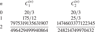
The details of the computation of the constants  $C_1^{(i)}$ and
 $C_2^{(i)}$, with
 $i = 0,1,2$, are given in appendix D. The results are summarized in table 1.

4. Discussion
The aim of this section is to discuss the results obtained for the effective surface viscosities. We compare our theoretical result for the effective surface dilatational viscosity to the semi-analytical solution obtained in a previous work (Lishchuk Reference Lishchuk2016). Finally, we discuss the range of validity of our theory with respect to finite surface concentrations, finite capillary numbers and imperfections of the particle surface.
With the help of (3.16), (3.17) and the results given in table 1, we obtain for the effective surface viscosities
 \begin{gather} \mu^{\mathcal{S}} \approx \frac{5}{3} \mu a \phi \left(1 + \frac{5}{4} \cos(\alpha) + 0.8912 \cos^2(\alpha) \right), \end{gather}
 \begin{gather} \kappa^{\mathcal{S}} \approx 5 \mu a \phi \left(1 + \frac{15}{8} \cos(\alpha) + 1.9036 \cos^2(\alpha) \right), \end{gather}
or, when using the surface concentration as defined in Lishchuk & Halliday (Reference Lishchuk and Halliday2009), i.e. (2.1),
 \begin{gather} \mu^{\mathcal{S}} \approx \frac{5}{3} \mu a \phi_L \left(1 + \frac{5}{4} \cos(\alpha) -0.1089 \cos^2(\alpha) \right), \end{gather}
 \begin{gather} \kappa^{\mathcal{S}} \approx 5 \mu a \phi_L \left(1 + \frac{15}{8} \cos(\alpha) + 0.9036 \cos^2(\alpha) \right). \end{gather}
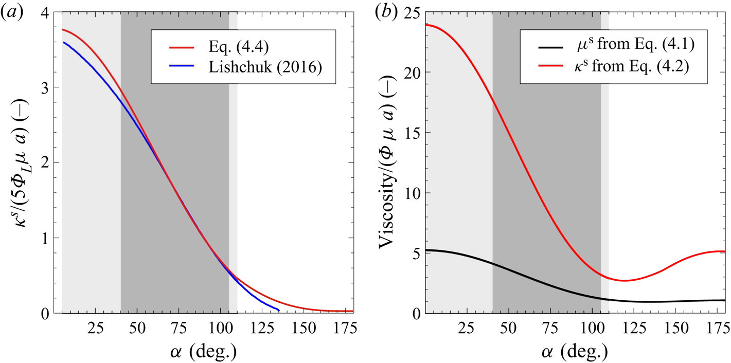
In figure 2(a), a comparison between (4.4) and the semi-analytical solution from Lishchuk (Reference Lishchuk2016) is shown. For a broad range of contact angles  $\alpha \in [40^{\circ }, 105^{\circ }]$ the deviation between the theoretical and the semi-analytical results is less than
 $5\, \%$ (dark grey region in figure 2a). The lighter grey areas correspond to a deviation of less than
 $10\,\%$. Similarly as in previous studies (Dörr & Hardt Reference Dörr and Hardt2015; Dörr et al. Reference Dörr, Hardt, Masoud and Stone2016; Eigenbrod et al. Reference Eigenbrod, Bihler and Hardt2018), the domain perturbation method leads to a better agreement with semi-analytical results for hydrophilic particles than for hydrophobic ones.
 $(a)$ Comparison between the prediction of (4.4) and the semi-analytical solution obtained in Lishchuk (Reference Lishchuk2016). The scaled dimensionless dilatational viscosity is shown as a function of the contact angle
 $\alpha$, where the definition of surface concentration from (2.1) is used. In the dark grey region the deviation between the two solutions is smaller than
 $5\,\%$, whereas the light grey region corresponds to deviations smaller than
 $10\,\%$.
 $(b)$ Dimensionless effective dilatational and shear viscosities as a function of the contact angle. In contrast to panel
 $(a)$, the physically correct surface concentration as defined in (2.2) is used. For the grey regions the same convention as in panel
 $(a)$ applies.

In figure 2(b), we plot the results of (4.1) and (4.2) over the contact angle  $\alpha$ of the particles. Again, the shaded areas refer to deviations of
 $5\, \%$ and
 $10\, \%$ between the analytical and the semi-analytical results for the dilatational viscosity. The dilatational viscosity shows a stronger dependence on the contact angle than the shear viscosity and also has a larger magnitude for all contact angles. Clearly, outside the shaded area towards superhydrophobic contact angles, both viscosities behave differently than expected (
 $\kappa ^{\mathcal {S}}, \mu ^{\mathcal {S}} \neq 0$, for
 $\alpha \to 180^{\circ }$).
Apart from the dimensionless surface viscosities discussed in figure 2( $b$), two additional dimensionless groups were shown to have an important influence on the evolution of a fluid interface, namely the dilatational and shear Boussinesq numbers (Brenner Reference Brenner1991)
 \begin{gather} \mathcal{B}_{\mu^{\mathcal{S}}} = \frac{\mu^{\mathcal{S}}}{\mu L} = \phi \left(\frac{5}{3} + \frac{25}{12}\cos(\alpha) + 1.4853 \cos^2(\alpha) \right) \frac{a}{L}, \end{gather}
 \begin{gather} \mathcal{B}_{\kappa^{\mathcal{S}}} = \frac{\kappa^{\mathcal{S}}}{\mu L} = \phi \left(5 + \frac{75}{8}\cos(\alpha) + 9.5178 \cos^2(\alpha) \right) \frac{a}{L}, \end{gather}
in which  $L$ is a characteristic dimension of the flow domain. Further, it might be required to evaluate the ratio of the two Boussinesq numbers. Up to
 $O(\cos ^2(\alpha ))$, we find
 \begin{equation} \frac{\mathcal{B}_{\kappa^{\mathcal{S}}}}{\mathcal{B}_{\mu^{\mathcal{S}}}} = \frac{\kappa^{\mathcal{S}}}{\mu^{\mathcal{S}}} = 3 + \frac{15}{8} \cos(\alpha)+0.6936 \cos^2(\alpha). \end{equation}
Equation (4.7) reveals that the ratio of the surface viscosities varies between 5 and 2.5 in the dark shaded region of figure 2, reflecting the range of validity of our theory.
Our theoretical model is limited to dilute suspensions in which  $\phi \ll 1$. By employing lattice Boltzmann simulations, Lishchuk & Halliday (Reference Lishchuk and Halliday2009) showed that the effective dilatational viscosity for interfacial particles having a contact angle of
 $\alpha = 90^{\circ }$ is valid up to surface concentrations of
 $\phi _L \approx 0.15$. We view this as a rough guideline for the validity range of our theory for all contact angles. Compared to volumetric suspensions, in which the classic expression due to Einstein is typically valid up to volume concentrations of 0.05 (Guazzelli & Morris Reference Guazzelli and Morris2011; Mewis & Wagner Reference Mewis and Wagner2012), higher-order corrections in the particle concentration appear less important. However, for fluid interfaces densely packed with particles the interfacial viscosities should show the same divergent behaviour as known for volumetric suspensions. For the dilatational viscosity of a particle-laden interface where the particles have a contact angle of
 $\alpha = 90^{\circ }$ this was studied by Lishchuk (Reference Lishchuk2014). A divergent behaviour similar to that of volumetric suspensions was obtained. We therefore hypothesize that our theoretical results for the dilute limit provide a lower bound to the effective viscosities and significantly underestimate these, especially for higher surface concentrations. In other words, our results probably represent the minimum influence of interfacial particles, a statement of relevance in different applications.
Our model is based on an asymptotically vanishing capillary number  $Ca$, leading to a flat fluid interface to leading order. In this paragraph, we discuss the influence of a pure straining flow on the interfacial deformation up to first order in
 $Ca$, while assuming a contact angle of
 $\alpha = 90^{\circ }$. The deformation of the fluid interface to first order can be computed on the basis of the zeroth-order solution for the velocity and pressure field. We do not aim at computing the exact shape of the fluid interface, but instead compute the hydrodynamic force/torque on the particle. This indicates whether the three-phase contact line between the surface of the particle and the two fluid phases is translated or rotated with respect to the coordinate origin. On the basis of the zeroth-order solution, i.e. (C 6) and (C 7) together with (2.6a,b), the force and torque acting on the immersed hemisphere of the interfacial particle can be computed as follows (
 $\boldsymbol {e}_x$ points into the fluid having the higher viscosity):
 \begin{gather} \boldsymbol{F} = \int_{{3 {\rm \pi}}/{2}}^{{\rm \pi}/{2}} \int_{0}^{\rm \pi} \left[\boldsymbol{\varPi}^{(0)} \boldsymbol{\cdot} \boldsymbol{e}_r\right]_{r = a}\ a^2 \sin(\theta) \,\mathrm{d}\theta\,\mathrm{d}\varphi = - 3 {\rm \pi}\mu a^2 ({\mathsf{E}}_{yy}^{\mathcal{S}} + {\mathsf{E}}_{zz}^{\mathcal{S}}) \boldsymbol{e}_x, \end{gather}
 \begin{gather} \boldsymbol{T} = \int_{{3 {\rm \pi}}/{2}}^{{\rm \pi}/{2}} \int_{0}^{\rm \pi} \left[\boldsymbol{r}\times(\boldsymbol{\varPi}^{(0)} \boldsymbol{\cdot} \boldsymbol{e}_r)\right]_{r = a}\ a^2 \sin(\theta)\,\mathrm{d}\theta\,\mathrm{d}\varphi = 0. \end{gather}
In agreement with physical intuition, a pure shear flow ( ${\mathsf{E}}_{yz}^{\mathcal {S}}\neq 0$,
 ${\mathsf{E}}_{yy}^{\mathcal {S}} = {\mathsf{E}}_{zz}^{\mathcal {S}} = 0$) and a planar straining flow (
 ${\mathsf{E}}_{yz}^{\mathcal {S}} = 0$,
 ${\mathsf{E}}_{yy}^{\mathcal {S}} = -{\mathsf{E}}_{zz}^{\mathcal {S}}$) do not lead to an interfacial deformation up to first order in
 $Ca$. Only a three-dimensional straining flow might cause a normal particle displacement with respect to the unperturbed fluid interface. In contrast to a particle translating along the interface, the hydrodynamic force is proportional to the squared particle radius, leading to a small relative interfacial deformation for small particles. Consequently, we believe that the effect of the capillary number on the effective rheological properties of the interfacial suspension is rather weak. The computation of the force and torque can be extended to contact angles deviating from
 $\alpha = 90^{\circ }$. However, we believe that the influence of the contact angle is rather small, since also for contact angles different from
 $90^{\circ }$ the only contribution to the force comes from a three-dimensional straining flow.
Another aspect that may limit the validity of the developed model is related to undulations of the three-phase contact line. Such undulations are caused by heterogeneities of the particle surface and may become prominent especially for small particles. The corresponding deformation of the fluid interface potentially causes deviations from the effective viscosities computed for a flat interface. While such effects cannot be excluded in general, there is experimental evidence that the contact-line undulations are negligibly small for micron-sized polystyrene beads, one of the most prominent particle types employed in context with small-scale flows. Stamou, Duschl & Johannsmann (Reference Stamou, Duschl and Johannsmann2000) and Park & Furst (Reference Park and Furst2011) showed that the perturbations of the contact line from a perfect circular shape are of the order of  $10^{-8}\ \textrm {m}$ in the case of micron-sized polystyrene beads, which should not significantly influence the validity of our results. It is worth mentioning that the influence of heterogeneities of the particle surface becomes more dominant at higher surface concentrations, mainly due to the above-mentioned capillary interaction.
5. Conclusion
In summary, we have studied the dissipation effects due to spherical particles adsorbed at the interface between two fluids with large viscosity contrast and computed the effective interfacial dilatational and shear viscosities. We limited our study to flat interfaces and small Reynolds numbers. Furthermore, the interfacial suspension was assumed to be dilute, allowing us to neglect the hydrodynamic, capillary and Brownian interactions between particles. Throughout this study, we made use of symmetry arguments stating that the physical situation of a particle attached to a flat interface is equivalent to that of a mirror-fused particle in the bulk of the fluid with higher viscosity. We employed the stress-averaging method of Batchelor (Reference Batchelor1970) for interfacial suspensions and found that the effective surface viscosities are solely determined by half of the stresslet acting on the mirror-fused particle.
The shape of the mirror-fused particle was modelled based on a domain perturbation method, where the contact angle  $\alpha$ of the more viscous fluid on the particle surface defines the particle shape. By applying the Lorentz reciprocal theorem (Lorentz Reference Lorentz1896) and solving the Stokes equations for the mirror-fused particle in a pure straining flow up to first order in the perturbation parameter
 $\beta = \cos (\alpha )$, we computed both interfacial viscosities of a Boussinesq–Scriven interface up to second order in
 $\beta$. We found that the dilatational viscosity is more sensitive to the contact angle than the shear viscosity. Further, the magnitude of the dilatational viscosity was shown to be larger than the magnitude of the shear viscosity, which is in agreement with experimental results obtained for particle-free fluid interfaces (Fox & Rock Reference Fox and Rock1946; Maru & Wasan Reference Maru and Wasan1979). Usually, in the corresponding articles, clean interfaces are considered, but recent results indicate that in practice, surface contaminations are very difficult to avoid (Peaudecerf et al. Reference Peaudecerf, Landel, Goldstein and Luzzatto-Fegiz2017). By comparing our results with the semi-analytical results of Lishchuk (Reference Lishchuk2016), we found that our perturbation approach agrees well with the semi-analytical data (deviation less than
 $5\,\%$) in a contact angle range between
 $40^{\circ }$ and
 $105^{\circ }$.
The results may prove useful in different contexts. First, they could help in the understanding of low-concentration particle-laden interfacial flows, especially the role of the contact angle in these flows. Second, in a similar way as with theories for the effective viscosity of a bulk suspension, our findings could pave the way to follow-up studies considering higher particle concentrations. This could enable understanding of the hydrodynamics of systems as complex as Pickering emulsions and liquid marbles.
Declaration of interest
The authors report no conflict of interest.
Appendix A. Contributions of ${U}^{eff}$ and ${\omega }^{eff}$ in the evaluation of the effective surface viscosities


We start our analysis with (2.5a,b) and derive the corresponding boundary conditions for a slightly deformed sphere up to second order in the small parameter  $\beta$, according to the solution procedure described in § 3. We therefore consider a surface parametrization as given in (3.1). The boundary conditions are then given by the following (more details can be found in appendix C):
 \begin{gather} \left. \boldsymbol{u}^{(0)}\right|_{r = a} = - \boldsymbol{\mathsf{E}} \boldsymbol{\cdot} \frac{\boldsymbol{r}}{r} a, \end{gather}
 \begin{gather} \left. \boldsymbol{u}^{(1)}\right|_{r = a} = \left( \boldsymbol{U}^{{eff},(1)} + \boldsymbol{\omega}^{{eff},(1)} \times \frac{\boldsymbol{r}}{r} a \right) - a f(\theta, \varphi) \left(\boldsymbol{\mathsf{E}} \boldsymbol{\cdot} \frac{\boldsymbol{r}}{r} + \left. \frac{\partial \boldsymbol{u}^{(0)}}{\partial r}\right|_{r = a} \right), \end{gather}
 \begin{align} \left. \boldsymbol{u}^{(2)}\right|_{r = a} &= \left( \boldsymbol{U}^{{eff},(2)} + \boldsymbol{\omega}^{{eff},(2)} \times \frac{\boldsymbol{r}}{r} a \right) - a f(\theta, \varphi) \left. \frac{\partial \boldsymbol{u}^{(1),{T}}}{\partial r}\right|_{r = a} \nonumber\\ &\quad + a f(\theta,\varphi) \left(\boldsymbol{\omega}^{{eff},(1)} \times \frac{\boldsymbol{r}}{r} - \left. \frac{\partial \boldsymbol{u}^{(1),{R}}}{\partial r}\right|_{r = a} \right) - a f(\theta, \varphi) \left. \frac{\partial \boldsymbol{u}^{(1),{S}}}{\partial r}\right|_{r = a} \nonumber\\ &\quad - a g(\theta, \varphi) \left(\boldsymbol{\mathsf{E}} \boldsymbol{\cdot} \frac{\boldsymbol{r}}{r} + \left. \frac{\partial \boldsymbol{u}^{(0)}}{\partial r}\right|_{r = a} \right) - \frac{a^2}{2} f(\theta,\varphi)^2 \left. \frac{\partial^2 \boldsymbol{u}^{(0)}}{\partial r^2}\right|_{r = a}, \end{align}
in which we used the expansions  $\boldsymbol {U}^{eff} = \beta \boldsymbol {U}^{{eff},(1)} + \beta ^2 \boldsymbol {U}^{{eff},(2)}$,
 $\boldsymbol {\omega }^{eff} = \beta \boldsymbol {\omega }^{{eff},(1)} + \beta ^2 \boldsymbol {\omega }^{{eff},(2)}$, as well as
 $\boldsymbol {u}^{(1)} = \boldsymbol {u}^{(1),{T}} + \boldsymbol {u}^{(1),{R}} + \boldsymbol {u}^{(1),{S}}$, i.e. the decomposition of the first-order velocity field into translational, rotational and pure straining contributions. As shown in § 2.1, the stresslet takes a major role in the calculation of the effective interfacial viscosities. We will therefore concentrate on the influence of the boundary conditions on the stresslet.
The boundary condition for the first-order velocity field is a superposition of the boundary conditions referring to an undeformed sphere translating and rotating with  $\boldsymbol {U}^{{eff},(1)}$ and
 $\boldsymbol {\omega }^{{eff},(1)}$, respectively, and a slightly deformed sphere in a pure straining flow. However, since the translational and rotational motion of an undeformed sphere do not contribute to the stresslet, it is sufficient to consider the pure-straining boundary condition for a slightly deformed sphere in the first-order contribution. Analogously, for the second order in
 $\beta$, i.e. (A 3), the first term in round brackets on the right-hand side does not need to be considered, since this also refers to an undeformed sphere in a constant translational and rotational velocity field. The following two terms correspond to a slightly deformed sphere up to first order of
 $\beta$ in pure translational (
 $\boldsymbol {U}^{{eff},(1)}$) and rotational (
 $\boldsymbol {\omega }^{{eff},(1)}$) motion (for comparison, see equations (3.9) and (4.3) in Brenner Reference Brenner1964), which contributes to the stresslet whenever at least one of these velocities is non-vanishing. The remaining terms correspond to a second-order slightly deformed sphere in a pure straining flow. In the following, we calculate the first-order effective velocities on the basis of a force and torque balance for the most general parametrization of a slightly deformed sphere.
To begin with, we expand the force  $\boldsymbol{F}$ and torque
 $\boldsymbol{T}$ in a power series in
 $\beta$ up to first order, leading to
 \begin{gather} \boldsymbol{F} \approx \boldsymbol{F}^{(0)} + \beta \boldsymbol{F}^{(1)}, \end{gather}
 \begin{gather} \boldsymbol{T} \approx \boldsymbol{T}^{(0)} + \beta \boldsymbol{T}^{(1)}. \end{gather}
For an undeformed sphere it is readily known that the rotation (translation) does not contribute to the force (torque) acting on it. We have
 \begin{gather} \boldsymbol{F}^{(0)} = -6 {\rm \pi}\mu a \boldsymbol{U}^{eff}, \end{gather}
 \begin{gather} \boldsymbol{T}^{(0)} = -8 {\rm \pi}\mu a^3 \boldsymbol{\omega}^{eff}. \end{gather}
In the first order of  $\beta$, the force and torque can be decomposed into translational, rotational and straining contributions. Using the solution for a translating and rotating slightly deformed sphere obtained by Brenner (Reference Brenner1964) and the solution procedure discussed in appendix C for a sphere in pure straining flow, the force and torque can be calculated using the following relations (Brenner Reference Brenner1964; Kim & Karrila Reference Kim and Karrila2013):
 \begin{gather} \boldsymbol{F} = - 4 {\rm \pi}\boldsymbol{\nabla}(r^3 p_{-2}), \end{gather}
 \begin{gather} \boldsymbol{T} = - 8 {\rm \pi}\mu \boldsymbol{\nabla}(r^3 \chi_{-2}), \end{gather}
in which  $p_{-2}$ and
 $\chi _{-2}$ are solid spherical harmonics of order
 $-2$ and part of Lamb's general solution (see appendix C for more details). After some algebra, the following identities are obtained:
 \begin{equation} \boldsymbol{F}^{(1)} = \boldsymbol{F}^{{T}, (1)} + \boldsymbol{F}^{{R}, (1)}+ \boldsymbol{F}^{{S}, (1)}, \end{equation}
with
 \begin{gather} \boldsymbol{F}^{{T}, (1)} = -6{\rm \pi} \mu a \left( \boldsymbol{U}^{eff} f_0 - \frac{1}{10} \boldsymbol{U}^{eff} \boldsymbol{\cdot} \boldsymbol{\nabla} \boldsymbol{\nabla} (r^2 f_2) \right), \end{gather}
 \begin{gather} \boldsymbol{F}^{{R}, (1)} = -6 {\rm \pi}\mu a^2 \boldsymbol{\omega}^{eff} \times \boldsymbol{\nabla}(r f_1), \end{gather}
 \begin{gather} \boldsymbol{F}^{{S}, (1)} = -4{\rm \pi} \mu a^2 \left(\frac{1}{14}\boldsymbol{\mathsf{E}}\,\textbf{:}\,\boldsymbol{\nabla}\boldsymbol{\nabla}\boldsymbol{\nabla}(r^3 f_3) - \frac{3}{2} \boldsymbol{\mathsf{E}}\boldsymbol{\cdot} \boldsymbol{\nabla}(r f_1) \right),\end{gather}
and
 \begin{equation} \boldsymbol{T}^{(1)} = \boldsymbol{T}^{{T}, (1)} + \boldsymbol{T}^{{R}, (1)}+ \boldsymbol{T}^{{S}, (1)}, \end{equation}
with
 \begin{gather} \boldsymbol{T}^{{T}, (1)} = 6 {\rm \pi}a^2 \mu \boldsymbol{U}^{eff} \times \boldsymbol{\nabla} (r f_1), \end{gather}
 \begin{gather} \boldsymbol{T}^{{R}, (1)} = -24 {\rm \pi}a^3 \mu \left(\boldsymbol{\omega}^{eff} f_0 - \frac{1}{10} \boldsymbol{\omega}^{eff}\boldsymbol{\cdot} \boldsymbol{\nabla}\boldsymbol{\nabla}(r^2 f_2) \right), \end{gather}
 \begin{gather} \boldsymbol{T}^{{S}, (1)} = 4 {\rm \pi}\mu a^3 \boldsymbol{\nabla} \times \left(\boldsymbol{\mathsf{E}} \boldsymbol{\cdot} \boldsymbol{\nabla}(r^2 f_2) \right), \end{gather}
in which  $f_k$ [
 $f_k = f_k(\theta ,\varphi )$] is the
 $k$th partial sum of the spherical-harmonics expansion of the shape function
 $f(\theta ,\varphi )$ (see (3.1)). After writing
 $\boldsymbol {U}^{eff} = \beta \boldsymbol {U}^{{eff},(1)}$,
 $\boldsymbol {\omega }^{eff} = \beta \boldsymbol {\omega }^{{eff},(1)}$ and inserting into (A 6), (A 7) and (A 10)–(A 17) we find that the force and torque balance is satisfied up to
 $O(\beta )$ if
 \begin{gather} \boldsymbol{U}^{{eff},(1)} = a \left(\boldsymbol{\mathsf{E}} \boldsymbol{\cdot} \boldsymbol{\nabla}(r f_1) - \frac{1}{21} \boldsymbol{\mathsf{E}}\,\textbf{:}\,\boldsymbol{\nabla}\boldsymbol{\nabla}\boldsymbol{\nabla}(r^3 f_3) \right), \end{gather}
 \begin{gather} \boldsymbol{\omega}^{{eff},(1)} = \tfrac{1}{2} \boldsymbol{\nabla} \times \left( \boldsymbol{\mathsf{E}} \boldsymbol{\cdot} \boldsymbol{\nabla}(r^2 f_2)\right). \end{gather}
It is worth mentioning that these results can be used to determine the trajectory of a slightly deformed sphere in a linear flow field. As already mentioned in § 3, the expansion  $f(\theta ,\varphi ) = \sin (\theta ) |\cos (\varphi )| = \sum _{k = 0}^{\infty } f_k$ only receives contributions from terms with
 $k = 0$ or
 $k$ even. Consequently, it follows that the first-order effective translational velocity vanishes. With (2.6a,b) and
 $f_2 = (-5/32) [3 \cos ^2(\theta )-1 + 3 (\cos ^2(\theta ) -1 ) \cos (2 \varphi ) ]$ it follows that
 $\boldsymbol {\omega }^{{eff},(1)} = 0$. Consequently, up to second order in
 $\beta$, the effective translational and rotational velocities do not need to be considered, i.e. it is sufficient to take the pure straining boundary condition into account.
Even though the effective translational and rotational velocities are zero in the present case, it might be useful for future studies to take the effect of a non-vanishing effective particle motion on the stresslet into account. Using
 \begin{equation} \boldsymbol{\mathsf{S}} \approx \boldsymbol{\mathsf{S}}^{(0)} + \beta \boldsymbol{\mathsf{S}}^{(1)} \end{equation}
and
 \begin{equation} \boldsymbol{\mathsf{S}}^{(1)} = \boldsymbol{\mathsf{S}}^{{T}, (1)} + \boldsymbol{\mathsf{S}}^{{R}, (1)} + \boldsymbol{\mathsf{S}}^{{S}, (1)}, \end{equation}
we find
 \begin{equation} \boldsymbol{\mathsf{S}}^{(0)} = \frac{20}{3} {\rm \pi}\mu a^3 \boldsymbol{\mathsf{E}}, \end{equation}
 \begin{align} \boldsymbol{\mathsf{S}}^{{T}, (1)} &= 2 {\rm \pi}\mu a^2 \left[\frac{1}{7} \boldsymbol{U}^{eff} \boldsymbol{\cdot} \boldsymbol{\nabla} \boldsymbol{\nabla} \boldsymbol{\nabla} (r^3 f_3) + \boldsymbol{U}^{eff} \boldsymbol{\cdot} \boldsymbol{\nabla} (r f_1) \boldsymbol{\mathsf{I}} \right. \nonumber\\ &\quad - \left. \frac{3}{2} \left(\boldsymbol{U}^{eff} \boldsymbol{\nabla} (r f_1) + \boldsymbol{\nabla} (r f_1) \boldsymbol{U}^{eff} \right) \right], \end{align}
 \begin{equation} \boldsymbol{\mathsf{S}}^{{R}, (1)} = - 2{\rm \pi} \mu a^3 \left[\boldsymbol{\nabla} (\boldsymbol{\omega}^{eff} \times \boldsymbol{\nabla}(r^2 f_2)) + \boldsymbol{\nabla} (\boldsymbol{\omega}^{eff} \times \boldsymbol{\nabla}(r^2 f_2))^T \right]. \end{equation}
The term corresponding to pure straining motion,  $\boldsymbol{\mathsf{S}}^{{S},(1)}$, is derived in appendix C. It should be noted that with the help of the boundary condition up to
 $O(\beta ^2)$ together with (A 21)–(A 24) and the reciprocal theorem (D 8), the stresslet for an arbitrary slightly deformed sphere can be calculated up to second order in
 $\beta$.
Appendix B. Underlying method for the computation of the effective interfacial viscosities
The purpose of this appendix is to introduce the underlying method for the computation of the effective interfacial viscosities, which is closely related to the work of Batchelor (Reference Batchelor1970). In this section we refer to figure 1(a,c) and therefore relate the suspension stresses inside the bulk (index:  $\mathcal {B}$) to effective interfacial properties (index:
 $\mathcal {S}$). Furthermore, we make use of assumption (iv) and neglect phase 2 in figure 1(a).
To start with, we may compute the volume-averaged stresses  $\langle \boldsymbol {\varSigma }_i \rangle _V$ referring to the bulk containing mirror-fused particles (
 $i = \mathcal {B}$) and the configuration reflecting effective interfacial suspension properties (
 $i = \mathcal {S}$), leading to
 \begin{gather} \langle \boldsymbol{\varSigma}_{\mathcal{B}} \rangle_V = \frac{1}{V_{\mathcal{B}}} \int_{V_{\mathcal{B}}} \boldsymbol{\varPi}\,\mathrm{d}V, \end{gather}
 \begin{gather} \langle \boldsymbol{\varSigma}_{\mathcal{S}} \rangle_V = \frac{1}{V_{\mathcal{S}}} \left[ \int_{V_{\mathcal{S}}} \boldsymbol{\varPi}\,\mathrm{d}V + \int_{A} \boldsymbol{\sigma}^{\mathcal{S}}\,\mathrm{d}S \right], \end{gather}
in which  $V_i$,
 $\boldsymbol {\varPi }$ and
 $\boldsymbol {\sigma }^{\mathcal {S}}$ are the total volume for
 $i = \mathcal {B}, \mathcal {S}$, the total bulk stresses and the deviatoric interfacial stresses, respectively. In light of figure 1, it follows that
 $V_{\mathcal {B}} = 2~V_{\mathcal {S}}$. Batchelor (Reference Batchelor1970) has shown that the right-hand side of (B 1) can be rewritten into a superposition of volume-averaged fluid properties and an additional term
 $\boldsymbol {\varSigma }_{\mathcal {B}}^{\mathcal {P}}$ reflecting the stresses due to the presence of particles:
 \begin{gather} \langle \boldsymbol{\varSigma}_{\mathcal{B}} \rangle_V = -\langle p \rangle_V \boldsymbol{\mathsf{I}} + 2 \mu \langle \boldsymbol{\mathsf{E}} \rangle_V + \frac{1}{V_{\mathcal{B}}}\boldsymbol{\varSigma}_{\mathcal{B}}^{\mathcal{P}}, \end{gather}
 \begin{gather} \langle \boldsymbol{\varSigma}_{\mathcal{S}} \rangle_V = -\langle p \rangle_V \boldsymbol{\mathsf{I}} + 2 \mu \langle \boldsymbol{\mathsf{E}} \rangle_V + \frac{1}{V_{\mathcal{S}}} \int_{A} \boldsymbol{\sigma}^{\mathcal{S}}\,\mathrm{d}S. \end{gather}
In the latter equation we have used the assumption that the presence of the particles modifies only the effective interfacial rheology, keeping the effective bulk properties unchanged. Comparing (B 3) and (B 4), the averaged fluid properties are of no further interest. However, a direct comparison between  $\langle \boldsymbol {\varSigma }_{\mathcal {B}} \rangle _V$ and
 $\langle \boldsymbol {\varSigma }_{\mathcal {S}} \rangle _V$ is not easily possible, since
 $\boldsymbol {\varSigma }_{\mathcal {B}}^{\mathcal {P}}$ is a three-dimensional matrix, whereas
 $\boldsymbol {\sigma }^{\mathcal {S}}$ is clearly two-dimensional, since it is just defined on the fluid interface. Nevertheless, introducing the energy dissipation helps solve this ‘formal’ problem. More precisely, the total energy dissipation of the interface reflecting the presence of particles coincides with the energy dissipation of mirror-reflected particles suspended in a bulk. We find, after computing the area average of the interfacial energy dissipation, that
 \begin{equation} \langle \boldsymbol{\sigma}^{\mathcal{S}}\rangle \,\textbf{:}\,\boldsymbol{\mathsf{E}}^{\mathcal{S}} = \frac{1}{2 A} \boldsymbol{\varSigma}_{\mathcal{B}}^{\mathcal{P}} \,\textbf{:}\,\boldsymbol{\mathsf{E}}. \end{equation}
Making further use of the results obtained by Batchelor (Reference Batchelor1970), we find that the particle stresses  $\boldsymbol {\varSigma }_{\mathcal {B}}^{\mathcal {P}}$ are closely related to the stresslet, leading to (2.8).
Appendix C. Solution of the Stokes equations for a slightly deformed sphere ($O(\beta )$) in a pure straining flow

In this section, we derive the solution of the Stokes equations together with the boundary conditions of (2.7a,b) on the basis of Lamb's general solution (e.g. Happel & Brenner Reference Happel and Brenner2012). Although in the main text we only use the solution from this appendix in the context of mirror-fused particles, we keep the calculation as general as possible, i.e. we use the parametrization of an arbitrary slightly deformed sphere. According to Brenner (Reference Brenner1964), we may limit our analysis to the first-order solution in the perturbation parameter  $\beta$.
The general parametrization of the surface of a slightly deformed sphere is given by
 \begin{equation} r_{\mathcal{P}} = a + \beta a f(\theta,\varphi), \end{equation}
in which  $\beta$ is assumed to be a small parameter. Equation (2.7a,b) then reads
 \begin{equation} \left. \boldsymbol{u}\right|_{r_{\mathcal{P}}} = - \boldsymbol{\mathsf{E}} \boldsymbol{\cdot} \frac{\boldsymbol{r}}{r} a \left[1 + \beta f(\theta,\varphi) \right]. \end{equation}
It is further assumed that the velocity field can be expanded in a perturbation series as
 \begin{equation} \boldsymbol{u} = \sum_{n = 0}^{\infty} \beta^n \boldsymbol{u}^{(n)}. \end{equation}
Correspondingly, every velocity field  $\boldsymbol {u}^{(n)}$ has to satisfy the Stokes equations. Every contribution
 $\boldsymbol {u}^{(n)}$ is now expanded into a Taylor series around
 $(r - a)$. In the same way as in Brenner (Reference Brenner1964), we obtain the following zeroth- and first-order boundary conditions:
 \begin{gather} \left. \boldsymbol{u}^{(0)}\right|_{r = a} = - \boldsymbol{\mathsf{E}} \boldsymbol{\cdot} \frac{\boldsymbol{r}}{r} a, \end{gather}
 \begin{gather} \left. \boldsymbol{u}^{(1)}\right|_{r = a} = - a f(\theta, \varphi) \left(\boldsymbol{\mathsf{E}} \boldsymbol{\cdot} \frac{\boldsymbol{r}}{r} + \left. \frac{\partial \boldsymbol{u}^{(0)}}{\partial r}\right|_{r = a} \right). \end{gather}
The former boundary condition refers to a sphere in a pure straining flow, for which the solution is readily known (e.g. Guazzelli & Morris Reference Guazzelli and Morris2011):
 \begin{gather} \boldsymbol{u}^{(0)} = - \frac{5 a^3}{2} \frac{\boldsymbol{r} \left(\boldsymbol{r} \boldsymbol{\cdot} \boldsymbol{\mathsf{E}} \boldsymbol{\cdot} \boldsymbol{r} \right)}{r^5} - \frac{a^5}{2} \left( \frac{\boldsymbol{\mathsf{E}} \boldsymbol{\cdot} \boldsymbol{r} + \boldsymbol{r}\boldsymbol{\cdot} \boldsymbol{\mathsf{E}}}{r^5} - \frac{5 \boldsymbol{r} \left(\boldsymbol{r} \boldsymbol{\cdot} \boldsymbol{\mathsf{E}} \boldsymbol{\cdot} \boldsymbol{r} \right)}{r^7} \right), \end{gather}
 \begin{gather} p^{(0)} = -5 \mu a^3 \frac{\boldsymbol{r} \boldsymbol{\cdot} \boldsymbol{\mathsf{E}} \boldsymbol{\cdot} \boldsymbol{r}}{r^5}. \end{gather}
Equation (C 5) then leads to
 \begin{equation} \left. \boldsymbol{u}^{(1)}\right|_{r = a} = 5 a f(\theta, \varphi) \left(\frac{\left(\boldsymbol{r} \boldsymbol{\cdot} \boldsymbol{\mathsf{E}} \boldsymbol{\cdot} \boldsymbol{r} \right)}{r^3} \boldsymbol{r} - \boldsymbol{\mathsf{E}} \boldsymbol{\cdot} \frac{\boldsymbol{r}}{r} \right). \end{equation}
According to Brenner (Reference Brenner1964), the equations (C 9–C 11) have to be evaluated and written in terms of three different surface spherical harmonics  $X_n, Y_n$ and
 $Z_n$, each of which is defined with respect to a specific angular function:
 \begin{gather} \sum_{n = 1}^{\infty} X_n = \frac{\boldsymbol{r}}{r} \boldsymbol{\cdot} \left. \boldsymbol{u}^{(1)}\right|_a = 0, \end{gather}
 \begin{gather} \sum_{n = 1}^{\infty} Y_n = - r \boldsymbol{\nabla} \boldsymbol{\cdot} \left( \left. \boldsymbol{u}^{(1)}\right|_a \right) = 5 a \left(\boldsymbol{\nabla} \left(\,f(\theta, \varphi)\right) \boldsymbol{\cdot} \boldsymbol{\mathsf{E}} \boldsymbol{\cdot} \boldsymbol{r} - 3 f(\theta,\varphi) \frac{\boldsymbol{r} \boldsymbol{\cdot} \boldsymbol{\mathsf{E}} \boldsymbol{\cdot} \boldsymbol{r}}{r^2} \right), \end{gather}
 \begin{gather} \sum_{n = 1}^{\infty} Z_n = \boldsymbol{r} \boldsymbol{\cdot} \boldsymbol{\nabla} \times \left( \left. \boldsymbol{u}^{(1)}\right|_a \right) =5 a \left(\boldsymbol{\mathsf{E}} \boldsymbol{\cdot} \frac{\boldsymbol{r}}{r}\right)\boldsymbol{\cdot} \boldsymbol{\nabla} \times \left(\,f(\theta,\varphi) \boldsymbol{r}\right) . \end{gather}
It follows directly that  $X_n = 0$,
 $\forall n$. We now expand
 $f(\theta , \varphi ) = \sum _{k = 0}^{\infty } f_k$ in an infinite sum of surface spherical harmonics and define
 \begin{gather} \sum_{n = 1}^{\infty}\ {_k}Y_n = 5 a \left(\boldsymbol{\nabla} \left(\,f_k\right) \boldsymbol{\cdot} \boldsymbol{\mathsf{E}} \boldsymbol{\cdot} \boldsymbol{r} - 3 f_k \frac{\boldsymbol{r} \boldsymbol{\cdot} \boldsymbol{\mathsf{E}} \boldsymbol{\cdot} \boldsymbol{r}}{r^2} \right), \end{gather}
 \begin{gather} \sum_{n = 1}^{\infty}\ {_k}Z_n = 5 a \left(\boldsymbol{\mathsf{E}} \boldsymbol{\cdot} \frac{\boldsymbol{r}}{r}\right)\boldsymbol{\cdot} \boldsymbol{\nabla} \times \left(\,f_k \boldsymbol{r}\right), \end{gather}
with the relations
 \begin{gather} \sum_{k = 0}^{\infty} \sum_{n=1}^{\infty}\ {_k}Y_n = \sum_{n=1}^{\infty}\, Y_n, \end{gather}
 \begin{gather} \sum_{k = 0}^{\infty} \sum_{n=1}^{\infty}\ {_k}Z_n = \sum_{n=1}^{\infty}\, Z_n. \end{gather}
It can be shown that for every fixed value of  $k$, only a finite number of terms in the sums of (C 12) and (C 13) are non-vanishing. After some algebra, the following relations are obtained:
 \begin{gather} {_k}Y_n = \begin{cases} \dfrac{5 a k (k-2)}{8 k^2 - 2} \boldsymbol{\mathsf{E}} \,\textbf{:}\,\left[4 \boldsymbol{\nabla} (\,f_k) \boldsymbol{r} + 2(k-2) f_k \dfrac{\boldsymbol{r} \boldsymbol{r} }{r^2}+ \dfrac{2}{k} r^2 \boldsymbol{\nabla}\boldsymbol{\nabla} (\,f_k)\right], & n = k-2,\\ \dfrac{30 a}{8k(k+1)-6} \boldsymbol{\mathsf{E}} \,\textbf{:}\,\left[\boldsymbol{\nabla} (\,f_k) \boldsymbol{r} - k(k+1) f_k \dfrac{\boldsymbol{r} \boldsymbol{r}}{r^2} + r^2 \boldsymbol{\nabla}\boldsymbol{\nabla} (\,f_k)\right], & n = k,\\ \dfrac{5 a(k+1)(k+3)}{4k(k+2)+3} \boldsymbol{\mathsf{E}} \,\textbf{:}\,\left[2 \boldsymbol{\nabla} (\,f_k) \boldsymbol{r} - (k+3) f_k \dfrac{\boldsymbol{r} \boldsymbol{r}}{r^2}- \dfrac{1}{k+1} r^2 \boldsymbol{\nabla}\boldsymbol{\nabla} (\,f_k)\right], & n = k +2,\\ 0, & \mathrm{else}, \end{cases}\end{gather}
 \begin{gather} {_k}Z_n = \begin{cases} \dfrac{5 a}{2k+1} \left[k \left(\boldsymbol{\mathsf{E}} \boldsymbol{\cdot} \dfrac{\boldsymbol{r}}{r} \right) \boldsymbol{\cdot} \left( \boldsymbol{\nabla}(\,f_k) \times \boldsymbol{r}\right)+ r \boldsymbol{\mathsf{E}} \,\textbf{:}\,\boldsymbol{\nabla} \left( \boldsymbol{\nabla} (\,f_k) \times \boldsymbol{r} \right) \right], & n = k-1,\\ \dfrac{5 a}{2k+1} \left[(k+1) \left(\boldsymbol{\mathsf{E}} \boldsymbol{\cdot} \dfrac{\boldsymbol{r}}{r} \right) \boldsymbol{\cdot} \left( \boldsymbol{\nabla}(\,f_k) \times \boldsymbol{r}\right)-r \boldsymbol{\mathsf{E}} \,\textbf{:}\,\boldsymbol{\nabla} \left( \boldsymbol{\nabla} (\,f_k) \times \boldsymbol{r} \right) \right], & n = k+1,\\ 0, & \mathrm{else.} \end{cases}\end{gather}
These identities can be verified in two steps: (i) the sum of all non-zero contributions on the right-hand sides of (C 16) and (C 17) have to be equal to the right-hand sides of (C 12) and (C 13); (ii) since  $_kY_n$ and
 $_kZ_n$ are surface spherical harmonics, it follows that
 $\nabla ^2 (r^n \lambda _n) = 0\ \forall n$, with
 $\lambda _n ={_k}Y_n,\ {_k}Z_n$.
Using the three solid spherical harmonics
 \begin{gather} {_k}p_{-(n+1)} = \frac{(2 n - 1) \mu}{(n+1) a} \left(\frac{a}{r} \right)^{n+1}\ {_k}Y_n ,\end{gather}
 \begin{gather} {_k}\phi_{-(n+1)} = \frac{a}{2(n+1)} \left(\frac{a}{r} \right)^{n+1} \ {_k}Y_n ,\end{gather}
 \begin{gather} {_k}\chi_{-(n+1)} = \frac{1}{n(n+1)} \left(\frac{a}{r} \right)^{n+1}\ {_k}Z_n,\end{gather}
the velocity and pressure field can be written as follows (Brenner Reference Brenner1964):
 \begin{align} \boldsymbol{u} &= \sum_{n = 1}^{\infty} \left[ \boldsymbol{\nabla} \times \left( \boldsymbol{r} \ {_k}\chi_{-(n+1)} \right) + \boldsymbol{\nabla} \ {_k}\phi_{-(n+1)} \vphantom{\frac{(n-2)}{2n(2n-1) \mu}}\right. \nonumber\\ & \left.\quad - \frac{(n-2)}{2n(2n-1) \mu} r^2 \boldsymbol{\nabla} \ {_k}p_{-(n+1)} + \boldsymbol{r} \frac{(n+1)}{n(2n-1)\mu} \ {_k}p_{-(n+1)} \right] , \end{align}
 \begin{equation} p = \sum_{n = 1}^{\infty} \ {_k}p_{-(n+1)}. \end{equation}
Using (C 16) and (C 17) we may rewrite (C 18)–(C 20) by replacing  $n$ with
 $k$ for all non-vanishing contributions:
 \begin{align} _k p_{-(k-1)} &= \frac{5(k-2)k(2k-5)}{2(k-1)(4k^2 -1)} \mu \left(\frac{a}{r} \right)^{k-1} \boldsymbol{\mathsf{E}}:\left[ 4 \boldsymbol{\nabla} (\,f_k) \boldsymbol{r} + 2(k-2) f_k \frac{\boldsymbol{r} \boldsymbol{r}}{r^2} \vphantom{\frac{(n-2)}{2n(2n-1) \mu}}\right. \nonumber\\ & \left.\quad + \frac{2}{k}r^2 \boldsymbol{\nabla} \boldsymbol{\nabla} f_k\right], \end{align}
 \begin{align} {_k} p_{-(k+1)} &= \frac{15}{2k^2+5k+3} \mu \left(\frac{a}{r} \right)^{k+1} \boldsymbol{\mathsf{E}}:\left[ \boldsymbol{\nabla} (\,f_k) \boldsymbol{r} - k(k+1) f_k \frac{\boldsymbol{r} \boldsymbol{r}}{r^2} \right. \nonumber\\ &\quad \left. + r^2 \boldsymbol{\nabla} \boldsymbol{\nabla} f_k \vphantom{\frac{\boldsymbol{r} \boldsymbol{r}}{r^2}}\right], \end{align}
 \begin{align} {_k} p_{-(k+3)} &= \frac{5(k+1)}{2k+1} \mu \left(\frac{a}{r} \right)^{k+3} \boldsymbol{\mathsf{E}}:\left[2 \boldsymbol{\nabla} (\,f_k) \boldsymbol{r} - (k+3) f_k \frac{\boldsymbol{r} \boldsymbol{r}}{r^2} \vphantom{\frac{1}{k+1}}\right. \nonumber\\ &\quad \left. - \frac{1}{k+1} r^2 \boldsymbol{\nabla} \boldsymbol{\nabla} f_k \right], \end{align}
 \begin{align} {_k} \phi_{-(k-1)} &= \frac{5k(k-2)a^2}{4(k-1)(4k^2-1)} \left(\frac{a}{r} \right)^{k-1} \boldsymbol{\mathsf{E}}\,\textbf{:}\,\left[ 4 \boldsymbol{\nabla} (\,f_k) \boldsymbol{r} + 2(k-2) f_k \frac{\boldsymbol{r} \boldsymbol{r}}{r^2} \vphantom{\frac{2}{k}}\right. \nonumber\\ &\quad \left. + \frac{2}{k}r^2 \boldsymbol{\nabla} \boldsymbol{\nabla} f_k\right], \end{align}
 \begin{align} {_k} \phi_{-(k+1)} &= \frac{15a^2}{(k+1)(8k(k+1)-6)} \left(\frac{a}{r} \right)^{k+1} \boldsymbol{\mathsf{E}}:\left[ \boldsymbol{\nabla} (\,f_k) \boldsymbol{r} - k(k+1) f_k \frac{\boldsymbol{r} \boldsymbol{r}}{r^2} \right. \nonumber\\ &\quad \left. + r^2 \boldsymbol{\nabla} \boldsymbol{\nabla} f_k \vphantom{\frac{\boldsymbol{r} \boldsymbol{r}}{r^2}}\right], \end{align}
 \begin{align} {_k} \phi_{-(k+3)} &= \frac{5(k+1)a^2}{8k(k+2)+6} \left(\frac{a}{r} \right)^{k+3} \boldsymbol{\mathsf{E}}:\left[2 \boldsymbol{\nabla} (\,f_k) \boldsymbol{r} - (k+3) f_k \frac{\boldsymbol{r} \boldsymbol{r}}{r^2} \vphantom{\frac{1}{k+1}}\right. \nonumber\\ &\quad \left. - \frac{1}{k+1} r^2 \boldsymbol{\nabla} \boldsymbol{\nabla} f_k \right], \end{align}
 \begin{align} {_k} \chi_{-k} &= \frac{5 a}{2k^3 - k^2 - k} \left(\frac{a}{r} \right)^{k} \left[ k \left(\boldsymbol{\mathsf{E}}\boldsymbol{\cdot} \frac{\boldsymbol{r}}{r} \right)\boldsymbol{\cdot} \left(\boldsymbol{\nabla}(\,f_k) \times \boldsymbol{r} \right) \right. \nonumber\\ &\quad + \left. r \boldsymbol{\mathsf{E}} \,\textbf{:}\,\boldsymbol{\nabla} (\boldsymbol{\nabla} (\,f_k) \times \boldsymbol{r}) \vphantom{\left(\boldsymbol{\mathsf{E}}\boldsymbol{\cdot} \frac{\boldsymbol{r}}{r} \right)}\right], \end{align}
 \begin{align} {_k}\chi_{-(k+2)} &= \frac{5 a}{2k^3 + 7k^2 + 7k+2}\left(\frac{a}{r} \right)^{k+2} \left[ (k+1) \left(\boldsymbol{\mathsf{E}}\boldsymbol{\cdot} \frac{\boldsymbol{r}}{r} \right)\boldsymbol{\cdot} \left(\boldsymbol{\nabla}(\,f_k) \times \boldsymbol{r} \right) \right. \nonumber\\ &\quad \left. - r \boldsymbol{\mathsf{E}} \,\textbf{:}\,\boldsymbol{\nabla} (\boldsymbol{\nabla} (\,f_k) \times \boldsymbol{r}) \vphantom{\left(\boldsymbol{\mathsf{E}}\boldsymbol{\cdot} \frac{\boldsymbol{r}}{r} \right)}\right]. \end{align}
The pressure up to first order in  $\beta$ is then found via
 \begin{gather} p_0 = \left. _k p_{-(k+3)}\right|_{k = 0}, \end{gather}
 \begin{gather} p_1 = \left. _k p_{-(k+1)}\right|_{k = 1} + \left. _k p_{-(k+3)}\right|_{k = 1}, \end{gather}
 \begin{gather} p_2 = \left. _k p_{-(k+1)}\right|_{k = 2} + \left. _k p_{-(k+3)}\right|_{k = 2}, \end{gather}
 \begin{gather} p_k = {}_k p_{-(k-1)} + {_k} p_{-(k+1)} + _k p_{-(k+3)}, \quad \mathrm{if}\ k>2, \end{gather}
 \begin{gather} p^{(1)} = \sum_{k = 0}^{\infty} p_k. \end{gather}
Following the same strategy, for the velocity field  $\boldsymbol {u}$ up to first order in
 $\beta$ we find
 \begin{equation} \boldsymbol{u}_{0} = \boldsymbol{\nabla} \times \left( \boldsymbol{r} \left. _k\chi_{-(k+2)}\right|_{k = 0} \right) + \boldsymbol{\nabla} \left(\left. _k \phi_{-(k+3)} \right|_{k = 0} \right) + \frac{1}{2 \mu} \boldsymbol{r} \left. _k p_{-(k+3)}\right|_{k = 0}, \end{equation}
 \begin{align} \boldsymbol{u}_{1} &= \boldsymbol{\nabla} \times \left( \boldsymbol{r} \left. _k\chi_{-(k+2)}\right|_{k = 1} \right) + \boldsymbol{\nabla} \left(\left. _k \phi_{-(k+3)} \right|_{k = 1} + \left. _k \phi_{-(k+1)} \right|_{k = 1} \right) \nonumber\\ &\quad + \frac{1}{2 \mu} r^2 \boldsymbol{\nabla} \left( \left. _k p_{-(k+1)} \right|_{k = 1} - \frac{1}{15} \left. _k p_{-(k+3)} \right|_{k = 1} \right) \nonumber\\ &\quad + \frac{2}{\mu} \boldsymbol{r} \left( \left. _k p_{-(k+1)}\right|_{k = 1} + \frac{2}{15} \left. _k p_{-(k+3)} \right|_{k = 1} \right), \end{align}
 \begin{align} \boldsymbol{u}_{2} &= \boldsymbol{\nabla} \times \left[ \boldsymbol{r} \left( \left. _k\chi_{-(k+2)}\right|_{k = 2} + \left. _k\chi_{-k}\right|_{k = 2} \right) \right] \nonumber\\ &\quad + \boldsymbol{\nabla} \left(\left. _k \phi_{-(k-1)} \right|_{k = 2} + \left. _k \phi_{-(k+3)} \right|_{k = 2} + \left. _k \phi_{-(k+1)} \right|_{k = 2}\right) \nonumber\\ &\quad - \frac{r^2}{28 \mu} \boldsymbol{\nabla} \left( \left. _k \phi_{-(k+3)} \right|_{k = 2} \right) + \frac{1}{2 \mu} \boldsymbol{r} \left( \left. _k p_{-(k+1)}\right|_{k = 2} + \frac{5}{14} \left. _k p_{-(k+3)}\right|_{k = 2} \right), \end{align}
 \begin{align} \boldsymbol{u}_{k} &= \boldsymbol{\nabla} \times \left[ \boldsymbol{r} \left( _k\chi_{-(k+2)} + _k\chi_{-k} \right) \right] + \boldsymbol{\nabla} \left( _k \phi_{-(k-1)} + _k \phi_{-(k+3)} + _k \phi_{-(k+1)} \right) \nonumber\\ &\quad - \frac{(k-4)}{2(k-2)(2(k-2) -1)\mu} r^2 \boldsymbol{\nabla} \left( _k p_{-(k-1)} \right) - \frac{(k-2)}{2k(2k-1) \mu} r^2 \boldsymbol{\nabla} \left( _k p_{-(k+1)} \right) \nonumber\\ &\quad - \frac{k}{2(k+2)(2(k+2)-1) \mu} r^2 \boldsymbol{\nabla} \left( _k p_{-(k+3)} \right) \nonumber\\ &\quad + \boldsymbol{r} \frac{k-1}{(k-2)(2(k-2)-1) \mu}\ {_k}p_{-(k-1)} + \boldsymbol{r} \frac{(k+1)}{k(2k-1) \mu}\ {_k}p_{-(k+1)} \nonumber\\ & \qquad \boldsymbol{r} \frac{k+3}{(k+2)(2(k+2) -1) \mu} \ {_k} p_{-(k+3)}, \quad \mathrm{if}\ k>2, \end{align}
 \begin{equation} \boldsymbol{u}^{(1)} = \sum_{k = 0}^{\infty} \boldsymbol{u}_{k}. \end{equation}
Equations (C 23)–(C 40) represent the first-order solution of the Stokes equations. The stresslet can be calculated in its most general form for Lamb's general solution and reads (Kim & Karrila Reference Kim and Karrila2013)
 \begin{equation} \boldsymbol{\mathsf{S}} = - \frac{2 {\rm \pi}}{3} \boldsymbol{\nabla} \boldsymbol{\nabla} \left(r^5 p_{-3}\right). \end{equation}
With the help of the foregoing derivations, we rewrite the  $O(\beta )$ contribution to the latter equation as
 \begin{equation} \boldsymbol{\mathsf{S}}^{(1)} = - \frac{2 {\rm \pi}}{3} \boldsymbol{\nabla} \boldsymbol{\nabla} \left[r^5 \left(\left. _k p_{-(k-1)} \right|_{k = 4} + \left. _k p_{-(k+1)} \right|_{k = 2} + \left. _k p_{-(k + 3)} \right|_{k = 0} \right)\right]. \end{equation}
Inserting (C 23)–(C 25), we find after some algebra that
 \begin{align} \boldsymbol{\mathsf{S}}^{(1)} &= 20
{\rm \pi} \mu a^3 \left(f_0 \boldsymbol{\mathsf{E}} - \frac{1}{21}
\left(\boldsymbol{\nabla} \boldsymbol{\nabla} \left(r^2 f_2
\right) :\boldsymbol{\mathsf{E}} \right) \boldsymbol{\mathsf{I}}
\right. \nonumber\\ &\quad \left. + \frac{1}{14}
\left(\boldsymbol{\mathsf{E}} \boldsymbol{\cdot} \boldsymbol{\nabla}
\boldsymbol{\nabla} \left(r^2 f_2 \right) +
\boldsymbol{\nabla} \boldsymbol{\nabla} \left(r^2 f_2
\right) \boldsymbol{\cdot} \boldsymbol{\mathsf{E}} \right) \right.
\nonumber\\ &\quad \left. - \frac{1}{189}
\boldsymbol{\nabla} \boldsymbol{\nabla} \boldsymbol{\nabla}
\boldsymbol{\nabla} \left(r^4 f_4 \right)
:\boldsymbol{\mathsf{E}} \right).
\end{align}
It should be noted that the latter equation holds for an arbitrary slightly deformed sphere. Interestingly, compared to the force and torque acting on a slightly deformed sphere (Brenner Reference Brenner1964), which are determined by  $f_0$,
 $f_1$ and
 $f_2$, the stresslet requires more detailed information about the shape of the particle, reflected in the term containing
 $f_4$.
Appendix D. Details on the solution of the Stokes equations around a mirror-reflected particle in pure straining
D.1. Zeroth-order solution
In this appendix we compute the effective surface viscosities for the case  $\alpha = 90^{\circ }$. This special case has already been studied by Lishchuk & Halliday (Reference Lishchuk and Halliday2009) and can therefore be considered as a benchmark for our approach. The stresslet of a spherical particle in a pure straining flow is readily known (e.g. Kim & Karrila Reference Kim and Karrila2013) and therefore the double contraction with the rate-of-strain tensor from (2.6a,b) can be evaluated, leading to
 \begin{equation} \boldsymbol{\mathsf{S}}^{(0)} \,\textbf{:}\,\boldsymbol{\mathsf{E}} = \frac{20 {\rm \pi}}{3} \mu a^3 \left[(\langle \boldsymbol{\nabla}^{\mathcal{S}} \boldsymbol{\cdot} \boldsymbol{u}^{\mathcal{S}} \rangle)^2 + (\langle \boldsymbol{\mathsf{E}}^{\mathcal{S}} \rangle)^2 \right], \end{equation}
from which the constants in (3.13) can be read off:
 \begin{equation} C_1^{(0)} = C_2^{(0)} = \frac{20}{3}. \end{equation}
The zeroth-order interfacial viscosities follow from (3.18) and (3.19):
 \begin{gather} \mu^{\mathcal{S}(0)} = \frac{5}{3} \phi \mu a , \end{gather}
 \begin{gather} \kappa^{\mathcal{S}(0)} = 5 \phi \mu a . \end{gather}
The zeroth-order solutions are identical to the results reported in Lishchuk & Halliday (Reference Lishchuk and Halliday2009) and therefore provide verification for the method presented in § 2.1.
Before we proceed to calculate the first-order corrections of the interfacial viscosities, we introduce the Lorentz reciprocal theorem (Lorentz Reference Lorentz1896) as a useful tool for the following analysis.
D.2. Lorentz reciprocal theorem
In its most general form, the Lorentz reciprocal theorem reads (Lorentz Reference Lorentz1896; Brenner Reference Brenner1991; Kim & Karrila Reference Kim and Karrila2013)
 \begin{equation} \int_{A_{\mathcal{P}}} \boldsymbol{u} \boldsymbol{\cdot} \bar{\boldsymbol{\varPi}} \boldsymbol{\cdot} \boldsymbol{n}\,\mathrm{d}A = \int_{A_{\mathcal{P}}} \bar{\boldsymbol{u}} \boldsymbol{\cdot} \boldsymbol{\varPi} \boldsymbol{\cdot} \boldsymbol{n}\,\mathrm{d}A, \end{equation}
in which ( $\boldsymbol {u}$,
 $\boldsymbol {\varPi }$) and (
 $\bar {\boldsymbol {u}}$,
 $\bar {\boldsymbol {\varPi }}$) satisfy the Stokes equations for the same flow geometry but with different boundary conditions. In this context, (
 $\bar {\boldsymbol {u}}$,
 $\bar {\boldsymbol {\varPi }}$) corresponds to a spherical particle with the boundary condition (3.3) and a vanishing velocity field at
 $r \to \infty$. The surface stress for this case reads
 $\bar {\boldsymbol {\varPi }} \boldsymbol {\cdot } \boldsymbol {n} = 3 \mu a\boldsymbol{\mathsf{E}} \boldsymbol {\cdot } ({\boldsymbol {r}}/{r})$ (Happel & Brenner Reference Happel and Brenner2012). Inserting the expression for the surface stress as well as (3.3) (here:
 $\tilde {\boldsymbol {u}} = - \boldsymbol{\mathsf{E}} \boldsymbol {\cdot } \boldsymbol {r} a/r$) into (D 5), we get
 \begin{equation} \left(3 \mu\, \int_{A_{\mathcal{P}}} \boldsymbol{u} \boldsymbol{n}\,\mathrm{d}A\right) :\boldsymbol{\mathsf{E}} = \left(- \int_{A_{\mathcal{P}}} \boldsymbol{r} \boldsymbol{\varPi} \boldsymbol{\cdot} \boldsymbol{n} \,\mathrm{d}A\right):\boldsymbol{\mathsf{E}}. \end{equation}
Since this equation needs to hold independently of the choice of  $\boldsymbol{\mathsf{E}}$, the two terms inside the brackets need to be identical. Calculating the symmetric and traceless parts of the terms inside the brackets, we find
 \begin{align} \int_{A_{\mathcal{P}}} \frac{3 \mu}{2} \left(\boldsymbol{u} \boldsymbol{n} + \boldsymbol{n} \boldsymbol{u} \right) - \mu (\boldsymbol{u} \boldsymbol{\cdot} \boldsymbol{n}) \boldsymbol{\mathsf{I}}\,\mathrm{d}A = - \int_{A_{\mathcal{P}}} \frac{1}{2} \left(\boldsymbol{r} \boldsymbol{\varPi} + \boldsymbol{\varPi} \boldsymbol{r} \right) \boldsymbol{\cdot} \boldsymbol{n} - \frac{1}{3} (\boldsymbol{r} \boldsymbol{\cdot} \boldsymbol{\varPi} \boldsymbol{\cdot} \boldsymbol{n})\, \boldsymbol{\mathsf{I}}\,\mathrm{d}A . \end{align}
For a rigid particle we have  $\boldsymbol {u} \boldsymbol {\cdot } \boldsymbol {n} = 0$. When we add
 $\int _{A_{\mathcal {P}}} \mu (\boldsymbol {u} \boldsymbol {n} + \boldsymbol {n} \boldsymbol {u})\,\mathrm {d}A$ to both sides of the latter equation, the right-hand side of this (D 7) corresponds to the negative stresslet. Therefore, we finally find
 \begin{equation} \boldsymbol{\mathsf{S}} = - \frac{5 \mu}{2}~\int_{A_{\mathcal{P}}} ( \boldsymbol{u} \boldsymbol{n} + \boldsymbol{n} \boldsymbol{u} )\,\mathrm{d}A . \end{equation}
In contrast to (2.9), in which the calculation of the surface stress requires detailed information on the velocity and pressure fields around the particle, (D 8) only involves an integration of the boundary conditions over the particle surface. It should be noted that the validity of (D 8) can be verified with the help of Lamb's general solution (Happel & Brenner Reference Happel and Brenner2012; Kim & Karrila Reference Kim and Karrila2013). After a lengthy calculation the expression of (C 41) is recovered.
D.3. First-order solution
Equations (3.3)–(3.5) display the successive solution process for slightly deformed spheres; i.e. the  $n$th order boundary condition is solely determined by the solutions up to
 $(n-1)$th order. Therefore, the first-order correction of the stresslet acting on a slightly deformed sphere can be calculated by inserting (3.4) in (D 8). Alternatively, the stresslet can be calculated according to (C 41), but requires the solution of the Stokes equations to first order in
 $\beta$. In appendix C we derive the first-order solution for a slightly deformed sphere in pure straining and provide an expression for the stresslet [see (C 43)]. Making use of these results, we find after a short calculation that
 \begin{equation} \boldsymbol{\mathsf{S}}^{(1)}\,\textbf{:}\,\boldsymbol{\mathsf{E}} = 20 {\rm \pi}\mu a^3 \left[\frac{35}{48} (\langle \boldsymbol{\nabla}^{\mathcal{S}} \boldsymbol{\cdot} \boldsymbol{u}^{\mathcal{S}} \rangle)^2 + \frac{5}{12} \left( \langle \boldsymbol{\mathsf{E}}^{\mathcal{S}} \rangle\right)^2 \right], \end{equation}
from which the following coefficients can be read off:
 \begin{equation} C_1^{(1)} = \frac{175}{12}, \quad C_2^{(1)} = \frac{25}{3}. \end{equation}
The first-order corrections to the effective surface viscosities then read
 \begin{gather} \mu^{\mathcal{S}(1)} = \frac{25}{12} \phi \mu a , \end{gather}
 \begin{gather} \kappa^{\mathcal{S}(1)} = \frac{75}{8} \phi \mu a . \end{gather}
It should be noted that, up to first order in  $\beta$, both definitions of the surface concentration [(2.1) and (2.2)] lead to the same effective viscosities.
D.4. Second-order solution
To obtain the second-order solution for the stresslet, we make use of the Lorentz reciprocal theorem from § 2. The second-order boundary condition at the surface of an undeformed sphere is given in (3.5). For reasons that will become clear later, we decompose (3.5) into two contributions, a first one proportional to the normal gradient of  $\boldsymbol {u}^{(1)}$, and a second one containing all other terms. When employing the reciprocal theorem (D 8), we start by evaluating the integral over all contributions that are not proportional to the normal gradient of
 $\boldsymbol {u}^{(1)}$ and find
 \begin{align} \boldsymbol{\mathsf{S}}^{(2)}\,\textbf{:}\,\boldsymbol{\mathsf{E}} &= - \frac{20 {\rm \pi}}{7} \mu a^3 \left[ 4 (\langle \boldsymbol{\nabla}^{\mathcal{S}} \boldsymbol{\cdot} \boldsymbol{u}^{\mathcal{S}} \rangle)^2 + 5 \left( \langle \boldsymbol{\mathsf{E}}^{\mathcal{S}} \rangle\right)^2 \right] \nonumber\\ &\quad + \frac{5}{2} \mu a \left[\int_{A_{\mathcal{P}}} f(\theta, \varphi) \left[\left. \frac{\partial \boldsymbol{u}^{(1)}}{\partial r}\right|_a \frac{\boldsymbol{r}}{r} + \frac{\boldsymbol{r}}{r} \left. \frac{\partial \boldsymbol{u}^{(1)}}{\partial r}\right|_a \right]\,\mathrm{d}A \right] \,\textbf{:}\,\boldsymbol{\mathsf{E}}. \end{align}
The quantity  $\boldsymbol {u}^{(1)}$ is written as an expansion in spherical harmonics (see (C 40)), reflecting the angular dependence of
 $f(\theta ,\varphi )$. We truncate the infinite sum by setting
 \begin{equation} \boldsymbol{u}^{(1)} \approx \sum_{k = 0}^{K} \boldsymbol{u}^{(1)}_k. \end{equation}
Inserting (D 14) into (D 13), and evaluating the remaining integral in (D 13) for  $K = 20$, we find
 \begin{align} \boldsymbol{\mathsf{S}}^{(2)}\,\textbf{:}\,\boldsymbol{\mathsf{E}} &\approx {\rm \pi}\mu a^3 \left[ \frac{1555263045342049}{165476499980288} (\langle \boldsymbol{\nabla}^{\mathcal{S}} \boldsymbol{\cdot} \boldsymbol{u}^{\mathcal{S}} \rangle)^2- \frac{60053874226845}{82738249990144}\left( \langle \boldsymbol{\mathsf{E}}^{\mathcal{S}} \rangle\right)^2 \right]. \end{align}
With the help of (3.13) and (3.15), the second-order coefficients are obtained as
 \begin{align} C_1^{(2)} \approx \frac{7975319135631907}{496429499940864} \approx 16.065, \quad C_2^{(2)} \approx \frac{1474603377122345}{248214749970432} \approx 5.941. \end{align}
To show that the 20 partial sums are sufficient to approximate the velocity field around the particle reasonably well, we plot the constants  $C_1^{(2)}$ and
 $C_2^{(2)}$ as a function of
 $K$ in figure 3. Figure 3(a) shows both coefficients as a function of
 $K$. The relative error of both coefficients decreases with increasing
 $K$ and falls below
 $0.1\,\%$ for
 $K = 20$, as shown in figure 3(b). All calculated coefficients are collected in table 1. The second-order corrections of the surface viscosities are computed for the two different definitions of the surface concentration, i.e. (2.1) and (2.2), as follows:
 \begin{gather} \mu^{\mathcal{S}(2)} \approx 1.4853 \phi \mu a, \quad \text{or} \quad \mu^{\mathcal{S}(2)} \approx -0.1815 \phi_L \mu a; \end{gather}
 \begin{gather} \kappa^{\mathcal{S}(2)} \approx 9.5178 \phi \mu a, \quad \text{or} \quad \kappa^{\mathcal{S}(2)} \approx 4.5179 \phi_L \mu a. \end{gather}
Convergence plot showing the dependency of the coefficients  $C^{(2)}_i\ (i = 1,2)$ referring to the second-order calculation of the stresslet of a slightly deformed sphere, on the summation limit
 $K$. (a) Absolute value of
 $C^{(2)}_i\ (i = 1,2)$ versus summation limit
 $K$. (b) Relative change of
 $C^{(2)}_i\ (i = 1,2)$ between
 $K+2$ and
 $K$ in per cent.