A crucial experiment in the historiography of Galileo's pendulum

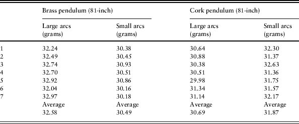
In a pioneering paper of 1974, Ronald Naylor claimed to have uncovered unequivocal and conclusive evidence that, in the light of his replication of experiments, Galileo's accounts of the experiments on which his claims concerning pendulum isochronism rested could not be supported.Footnote ¹¹ Interestingly, Naylor based his indictment on a ‘historiographically correct’ reconstruction of Galileo's pendulum experiments. Naylor ingeniously used a replica of Galileo's water clock to measure periods of oscillation, not a modern stopwatch. Hence Naylor's time measurements would have been available to Galileo. The water clock had been devised by Galileo to measure the time of fall of balls rolling down an inclined plane, as he famously recounts in Two New Sciences. By collecting in a beaker the water flowing through a narrow pipe placed at the bottom of a large tank, and subsequently weighing the water, Naylor measured the periods of three back-and-forth oscillations of brass and cork pendulums eighty-one inches long. He repeated the procedure for small and large oscillations in both cases and came up with the data summarized in Table 1.

Table 1.

The data of Naylor's experiments with brass and cork pendulums. Naylor does not say how he weighed the water collected in the beaker, but since the experiments were carried out in the early 1970s I speculate that he used a mechanical device, such as a scale with a movable index. The brass pendulum is faster for smaller arcs, whereas, puzzlingly, the opposite is true for the cork pendulum

Naylor comments on the data in Table 1 as follows:

Thus Naylor became convinced that Galileo's thesis about the isochronism of the simple pendulum was unsupported by experiment and that at the very least Galileo is guilty of misrepresenting the empirical evidence. Furthermore, Naylor was baffled by the puzzling result that while the brass pendulum is faster for smaller arcs, as expected in the light of our present knowledge, the opposite seems to be true for the cork pendulum.

I believe that Naylor's conclusions are untenable. They are the result of faulty premises in his argument and of artefacts in his pendulum set-up. To understand why, one needs to clear away the puzzling result of the brass versus cork pendulums, delve into the question of measurement of weights with a balance, and finally extend analysis of the measurement of weights to pendulum isochronism. The first two tasks are addressed in the ‘Supporting document’ to this paper. With respect to the final task, one can ask how to categorize the forms of the periodicities displayed by a pendulum swinging through small and large arcs. Are they equal and, if so, in what sense of equality? Unlike the discrete weights on a balance, whose phenomenal relation to each other can be categorized under the equilibrium/disequilibrium dichotomy, pendulum periodicities are continuous phenomena not easily subsumed under any bipolar categorization. They tend to change continuously over time. Below in ‘Galileo's investigative pathways around the pendulum’, I will show the emergence in real experiments of a discrepancy, a gradual tendency towards the inequality of pendulum periodicities. For the time being, I will discuss pendulum periodicities with the help of a computer model.

The discrepancy is a nonlinear phenomenon emerging in pendulum motions on a sufficiently large temporal scale. The discrepancy transcends ordinary dichotomies such as that of equality/inequality, which are evaluated at a smaller scale, that of the fundamental period. The discrepancy can be illustrated by showing the motions of the pendulum with respect to an ideal ‘simple pendulum’ through phase diagrams. A phase diagram shows the relation of the angular position of the motion of a real pendulum with respect to the angular position of the motion of the ideal simple pendulum evolving under the same physical constraints and from the same initial conditions. Consider the following two equations:

where q is the angular position of the pendulum bob, g is the gravity constant at the surface of the earth, and r is the length of the string (the ellipses stand for further terms, due to such physical constraints as air resistance, that are irrelevant here.)Footnote ¹³ The first, nonlinear, equation represents the motion of the real pendulum where the gravity component is compounded with the sine function of the angular position. The second, linear, equation represents the motion of the simple ideal pendulum where the sine function has been idealized away and replaced by a linear function. The ratio of g to r indirectly expresses the fundamental period of the pendulum.

Now imagine a real pendulum and its ideal counterpart. If an ideal pendulum could be built, the discrepancy would be evident. This is possible but difficult. However, a computer model can be constructed that calculates both the real and ideal pendulums together under the same parameters. This allows the discrepancy to be observed. Figure 1 shows two phase diagrams of the discrepancy obtained by calculating the motions of a real pendulum and its ideal counterpart from the same two sets of initial conditions. The vertical axis is the coordinate of the angular position of the ideal pendulum. The horizontal axis is the coordinate of the angular position of the real pendulum.

Figure 1.

Two phase diagrams of the discrepancy obtained by simulating the motions of a real pendulum and its ideal counterpart from the same two sets of initial conditions. The first set, Diagram 1, is from rest and an initial angle of 80°. The second set, Diagram 2, is from rest and an initial angle of 25°. The time of the simulation is 90 seconds. At time zero both pendulums are at rest at the same position, 80° in the first case, 25° in the second case. Time is not represented as a coordinate in the phase diagrams. To read the diagram, start from the first point (close to the grey arrows) and follow the line along which the phase between the two pendulums changes. Any point on the phase line shows the angular position of the real pendulum in relation to the angular position of the ideal pendulum. If the real pendulum behaved exactly like its ideal counterpart the phase diagram would be a line inclined at 45° (the dotted line in the first diagram but not represented in second diagram for clarity). Hence the more flattened the phase diagram seems around the direction of 45° the more ideal can be considered the real pendulum. Phase Diagram 2 represents such a case. The oval looks more flattened around the 45° direction, thus the real pendulum oscillates more closely to its ideal counterpart. The phase line resembles a spiral. Each gyration is a complete oscillation of the pendulum. There are as many oscillations in the ninety seconds of the simulation as gyrations in the phase diagram. For this simulation the material data of the pendulums were as follows: bob mass 58 g, bob material lead, string diameter 1 mm.

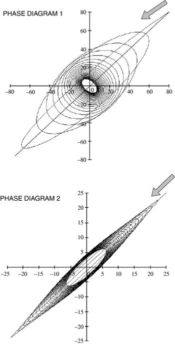
Phase Diagram 1 (Figure 1) is easier to read since the discrepancy is more pronounced. The ‘oval’, the shape of the gyration representing one oscillation, grows fatter and fatter, initially lying closer to the 45° direction, and later, as the motion progresses, gradually and continuously losing its oval character to become a quasi-circle showing no preferential directionality, and finally, towards the end of the simulation, assuming once again a pronounced directionality, perpendicular to the 45° direction. Now consider Phase Diagram 2. Since the motions begin at a smaller angle (only 25°) the discrepancy does not show the gradual progression of directionality from ~45° to ~135° (that is, more or less perpendicular to ~45°). In this second case the discrepancy remains stable, flattened along the 45° direction.

The ideal pendulum cannot be seen in reality, at least not under the circumstances of Galileo's experiments. However, if one lets the two real pendulums swing together from the two different angles, 80° and 25°, one can see the discrepancy in action, not between the real and ideal pendulums, but between two real pendulums. See Phase Diagram 3 in Figure 2.

Figure 2.

The discrepancy emerging between two real pendulums rather than between real and ideal pendulums.

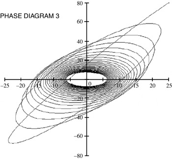
A fundamental feature common to all three phase diagrams is the stabilization of the discrepancy through time. This is displayed in the diagrams as the limit towards which the gyrations tend. The density of gyrations becomes greater around a limit gyration. In all cases there clearly emerges a limit gyration which marks off an area into which the pendulums do not enter. This means that the discrepancy between real pendulums, subject to physical constraints such aerodynamic resistance, does not explode by becoming ever larger. It also emphasizes the emergent character of the discrepancy. The emergent features of this discrepancy are not discernible from measurements of a single period of oscillation, nor from a few periods of oscillation, as was done by Naylor. They require a new observational act of ‘balancing’ periodicities from a large-scale temporal perspective.

Galileo of course had at his disposal neither the calculus needed to write down the equations of motion, nor the computers needed to calculate the phase diagrams. But, as shown below in ‘Galileo's investigative pathways around the pendulum’, with the help of videos of real experiments, the discrepancy is an obvious visual attribute of real pendulum motion that can easily be perceived. Galileo did not categorize the world according to the contrast between isochronism and non-isochronism presupposed in the relevant secondary literature. That duality is the product of later developments in the mathematical–physical sciences, notably the rational mechanics of the late seventeenth century and the eighteenth. Isochronism is not a Galilean word. Galileo's expressions for time-forms of pendulum periodicities are revealing.Footnote ¹⁴ As we shall see below in ‘Galileo's investigative pathways around the pendulum’, he speaks generally in terms of pendulums ‘going under the same time’. The expression betrays the large time-scale approach to the pendulum. He clearly perceives the regular and smooth evolution of the time-form of pendulum periodicities, the slowly varying nature of the gyrations. To learn this new mode of perception is to learn a new act of ‘balancing’ that challenges the procedure of the bilancetta, Galileo's exquisite precision balance, described in the ‘Supporting document’. Weights on Galileo's bilancetta have been fixed in quantity. This fixing happened at the time when the beaker collecting water was removed from under the tap of the water tank. Thus weights on the bilancetta are unlike the smoothly evolving discrepancy. It is impossible to weigh the discrepancy because it cannot be frozen in time. Galileo can only learn how to perceive it in time. But whence the emergence of the discrepancy? The next section illustrates how the discrepancy emerges as part of the perception of the pendulum's temporal periodicities.

Pendulum discrepancy as an attribute of periodicity perception

The previous section discussed the discrepancy as an objective phenomenon emerging in pendulum motions. This section discusses the discrepancy as a subjective attribute of the perception of the time-form of pendulum periodicity. Perception of pendulum periodicity depends on positioning one's body accurately in the scene of the experiment. So before discussing perception, I illustrate the sequence of body movements and positioning that I learnt while replicating Galileo's pendulum experiments. Here I present pictures (Figure 3a–g) showing body positioning in a realistic setting generated with computer imaging software. The sequence is presented cinematically, in a frame-by-frame sequence. Each picture is accompanied by a brief description. The whole sequence covers the execution of movements from the grabbing of the pendulum bob to its release and eventually to the final positioning that optimizes the perception of pendulum periodicity. The release of two bobs can be easily achieved, but the possible difference between the angles is limited by the span of the achievable widening of the operator's arms. If more is desired then a second operator must enter the scene and release a second bob simultaneously with the first operator.

Figure 3a.

The operator reaches the side of the gallows-like structure and grabs the ball. Subsequently the operator takes up the position shown in the picture, extending the string of the pendulum as far as the angle desired while gradually putting the string under tension.

Figure 3b.

The operator ‘takes aim’, as it were, trying to position the hand which grabs the bob in such a way that the motion of the pendulum remains as much as possible in a non-rotating plane. Since the pendulum is attached to a string, its oscillation plane has a tendency to deviate uncontrollably. Yet to a certain extent the operator learns how to sense and prevent this effect before releasing the bob.

Figure 3c.

After releasing the bob, while still looking at the bob, the operator abandons the initial position and reaches the centre of the experiment stage.

Figure 3d.

The operator checks his/her alignment with the plane ideally traced in space by the gallows-like structure of the pendulum support. The operator must quickly identify the right spot.

Figure 3e.

The operator subsequently assumes a squatting position, since otherwise a perspective angle from above makes the perception of the oscillation of the pendulum bob more difficult.

Figure 3f.

Here the frame taken from behind suggests as accurately as possible the exact angle of observation that the operator must take up.

Figure 3g.

In order to observe the emergence of the discrepancy phenomenon the operator needs to release two bobs at the same time from different positions; only one is shown in the picture.

Galileo does not report whether the pendulum experiments were carried out alone or with assistants. I tried both options and both can work well, though the first obviously only works within the constraints just mentioned. An easy way for the two operators to synchronize their actions is by counting aloud integers and by releasing the bobs at a count agreed upon in advance. One can speculate that if Galileo did not seek the help of assistants for pendulum experiments with strings of the order of between three and five braccia in length, the lengths he indicates on many occasions, then he would have been unable to release two bobs from angles separated by more than approximately forty-five degrees. We now turn to the discussion of perception.

Since the time-form of pendulum periodicities is always an oscillation whose amplitude tends to decrease over time, we can represent the time-form by means of Fourier spectrum analysis. This means of representation of the time-form allows us to investigate how the physical constraints shape the spectrum of the component frequencies, or periods. Consider Figure 4. Starting from rest, a two-ounce lead bob swings from two different initial angles, a small angle and a larger one. The motion is smoothly slowed down by aerodynamic resistance. However, aerodynamic resistance has another formidable effect that only spectrum analysis reveals. The next figure offers a Fourier analysis of motions of the same pendulum after removing the effect of aerodynamic resistance. This is not physically easy to realize but easy to derive from computer modelling. Consider Figure 5. While the fundamental period of the pendulum swinging from the smaller angle has remained virtually the same, that of the pendulum swinging from the larger angle has increased from less than to more than 3.5 seconds. Fourier analysis shows that a dramatic effect of aerodynamic resistance is to make the two fundamental periods coincide. The air resistance to the bobs and strings slows the pendulums such that the two will move with the same fundamental period. What does this mean for the discrepancy as a subjective attribute of perception of the time-form of pendulum periodicity? Aerodynamic force is responsible for shaping the spectrum of the time-form of pendulum periodicity in such a way that we lose our perceptual grip on the fundamental period of the pendulum. If we could observe the two pendulums in a vacuum swinging from the two different initial angles, we would perceive two fundamental periods, just as when we perceive two musical tones different in pitch as forming one interval, a two-note chord. Now, because of aerodynamic force the ‘visual tones’ of the two pendulums are fused into one single ‘visual tone’, one single ‘visual pitch’. Aerodynamic resistance makes the two pendulums appear visually in unison.

Figure 4.

The Fourier spectrum of the time-form of pendulum periodicities. The white square symbols represent the spectrum of a pendulum swinging from an initial angle of 80°, while the black dot symbols represent the spectrum of the same pendulum swinging from an initial angle of 20°. The horizontal axis is the coordinate of the period of the component of the spectrum. The vertical axis is the coordinate of the amplitude of the period component of the spectrum (the scale of the vertical axis is irrelevant for present purposes). The pendulum has a fundamental period, the period given by the peak among the frequency amplitudes, of between 3 and 3.5 seconds. The horizontal axis represents the time of the component period of the spectrum, not the real time of the phenomenon. For better legibility, the diagram shows time instead of frequency because the durations of the component periods are longer than one second.

Figure 5.

The Fourier spectrum of the time-form of pendulum periodicities. The same situation as in Figure 4, except that aerodynamic resistance has been removed. For clarity, grid lines have been omitted. The minor peak is the pendulum swinging from the smaller angle, whose fundamental period remains virtually the same.

The perception of the time-form of pendulum periodicity experienced when we observe two real pendulums swinging from two different angles is a visual unison formed by the two pendulums each swinging with a different timbre but the same pitch. The next section brings abstract analysis to life by discussing real experiments and by inviting the reader to examine videos of the discrepancy of real pendulums as Galileo would have been seen it.

Galileo's investigative pathways around the pendulum: (1) in the scene of experience

This section deals with my reconstruction of Galileo's experiments. I will focus on the outcomes of the experiments, on the activities that constitute the outcome of an experiment, and on their pointing to investigative pathways in the context of Galileo's early researches. An experiment is hardly an isolated event, but more like the performance of a set of interrelated activities in a scene of experience. However, it is not always easy to define or design the activities in advance. At times they are dictated by the very nature of the artefact around which they begin to develop.

I assembled a slender and light wooden frame in the form of a gallows (consult the ‘Supporting document’ for further details). The main vertical post I made moveable so I could quickly raise the horizontal arm to have more vertical room for longer pendulums. I prepared the horizontal arm with holes and hooks, so that I could hang pendulums at different distances from each other. I wanted to observe two pendulums swinging behind each other. In this way I made sure that I had a good perspective, that I could see two equal pendulums marching synchronously and in parallel, and moreover that my point of view was freely movable all round. Figure 6a shows the scene of the pendulum experience. Figure 6b shows a detail of the apparatus. I begin by recounting how I measured the lengths of two equal pendulums, or rather how I decided that my two pendulums had the same length.

Figure 6a.

The scene of the pendulum experience. The wooden gallows-like frame is at the centre. Behind it is a white backdrop for improving direct observations and also shooting film. The use of modern electronics is explained in Appendix 2 of Paulo Palimieri, Re-enacting Galileo's Experiments (Lewiston N.Y., 2008).

Figure 6b.

A detail of the upper part of the pendulum apparatus. The horizontal bar is made of Plexiglas. The load cells used for measurements of the tension in the strings can be seen on the Plexiglas bar (see Palimieri, Re-enacting Galileo's Experiments, Appendix 2).

To begin I cut two hemp strings of the same length (about ninety-two inches).Footnote ¹⁵ First I cut one and then the second after making their ends coincide. I suspended two pendulums made of hemp strings knotted to two one-ounce lead balls, adjusting the knots until I was satisfied by visual inspection that the two pendulums were of the same lengths.Footnote ¹⁶ The pendulums were removed from the perpendicular and let go at the same instant. They started losing synchronism after a short while, contrary to my expectations. So I thought that there might be something wrong with the apparatus or with the way I let the bobs go. I repeated the test with the same results. I tried from the other side of the apparatus with the same results. Finally it dawned on me that the lengths of the pendulums might in fact not be the same. By ‘length of the pendulum’ I mean the resulting length of the string plus the radius of the ball to which the bob is attached, once the pendulum has been hung from the frame. The operation of mounting the pendulum affects its length. In fact visual inspection failed as a criterion of equality for the lengths of pendulums.

There is no way of ensuring the two lengths are the same, other than letting the pendulums swing together for as long a time as possible, and observing that they will oscillate synchronously by keeping pace with each other. Again, the determination of a ‘sameness’ in the measurement process, in this case the sameness of length, requires an indefinite process, in fact an indefinite time. The two pendulums function together as a combined accumulator of the delays due to the inevitable difference in the lengths of the pendulums. So in order to guarantee that pendulum experiments are significant, one has to work patiently until one is satisfied that for an arbitrarily defined interval of time the pendulums will swing synchronously. I finally settled on a ‘reasonable’ time window of five minutes. Beyond that time limit I knew I would have to expect the results to become less and less reliable since the pendulums would slowly start losing synchronism. I spent my first morning in the scene of experience working out this problem.

Since the pendulums are supposedly identical, by ‘oscillating synchronously’ I simply mean that they appear to the observer to move together. ‘Togetherness’ here is unproblematic, because the two pendulums will always have to be in the same position at the same time.

Videos 1 to 4 (‘The length of the pendulum’) document the phenomenon of the lengths of the pendulums. They show longer and longer synchronism between two pendulums of ‘equal’ lengths. I achieved this result during my first morning in the scene of experience. The astonishing fact is that pendulums will always tend to go out of synch and do so relatively quickly. How quickly? When I started, I had in mind the hundreds of oscillations that Galileo seems to claim to have counted.Footnote ¹⁷ Galileo approximately indicates pendulum lengths in the range of four to five braccia – that is, two to three metres, depending on the choice of equivalent of Galileo's braccio. With these lengths, it was difficult for me to observe more than about one hundred ‘good’ oscillations, since the time window allowed by my two ‘equal’ pendulums was about five minutes (about one hundred oscillations for pendulums of ninety-two inches).

This does not imply that it is impossible in principle to fine-tune the lengths of the pendulums until they swing more than one hundred oscillations synchronously. But it does mean that the fine-tuning becomes more difficult and tedious, since there are obvious limitations in the way the hands of a human observer operate while, for example, trying to adjust a knot around the hook of the lead ball.Footnote ¹⁸ When doing the adjusting the operator cannot be helped by visual inspection, since the lengths of the pendulums will always tend to look the same.

Furthermore, there is another practical limitation to the manual procedure of adjusting the lengths. Hemp strings tend to coil and are also very flexible. In order to straighten them one has to apply some tension, which will, however, tend to extend them a little. Adjustment must be done by trial and error. Tension in the string is an ineliminable problem that the pendulum experimenter learns how to live with pretty quickly. In fact, as I have realized, when grabbing the lead balls in preparation for a launch the operator is constantly adjusting, more or less consciously, the tension applied to the strings. This tension does not sensibly affect the outcome of the experiment, as I have concluded, yet creates a kind of anxiety that the outcome will in fact be affected.

We can experiment virtually with the effects of slight differences in the lengths of supposedly equally long pendulums with the help of a computer model of the pendulums used in real experiments.Footnote ¹⁹ I ran a few simulations and noticed that in order to end up with a visually discernible lack of synchronism between the two pendulums, after a number of oscillations comparable to that of Videos 1 to 4 (‘The length of the pendulum’), a difference of about five millimetres is required (see S-Video 1, ‘Two lengths’). This suggests that once the pendulums are mounted on the wooden frame the observer's perspective determines a margin of error in the estimated equality of the lengths of the pendulums of at least about that size.

Why do pendulums stop swinging? The question is far from naive, since resistance due to impediments, such as air and/or mechanical friction, might not be the sole or even the principal factor responsible for the slowing of pendulums. In early seventeenth-century Padua, Aristotelian natural philosophers such as, for example, Galileo's friend Cesare Cremonini (1550–1631) would have assumed that the medium was responsible for keeping the pendulum going, not for slowing it down. Galileo came up with an ingenious hypothesis, as we will now see.

Galileo's investigative pathways around the pendulum: (2) the artefact's modes

In a fascinating passage in Dialogue on the Two Chief World Systems (1632), Galileo expounds an elaborate theory of the intrinsic tendency of pendulums to slow down and eventually stop regardless of all external impediments.Footnote ²⁰ Galileo also draws a figure of the shape of an oscillating pendulum made with a bob and a rope (Figure 7). He argues that if the pendulum's suspension is a corda (rope), a thicker and heavier suspension than the thin spago (string), or spaghetto, as generally reported in other texts, then the rope's parts behave like many pendulums distributed along the rope.Footnote ²¹ These will have their own well-determined higher and higher frequency as their distance from the centre of oscillation becomes smaller and smaller. Therefore, Galileo argues, they will slow down the oscillating bob, since the latter will be ‘restrained’ by the many pendulums of which the rope really consists and which will want to oscillate faster than the bob. This effect, Galileo continues, will be even more manifest to the senses if the rope is replaced with a chain. Thus, Galileo concludes, all pendulums will inevitably stop, even if all external impediments are removed.

Figure 7.

The non-rectilinear shape that a pendulum made with a rope would show during an oscillation.

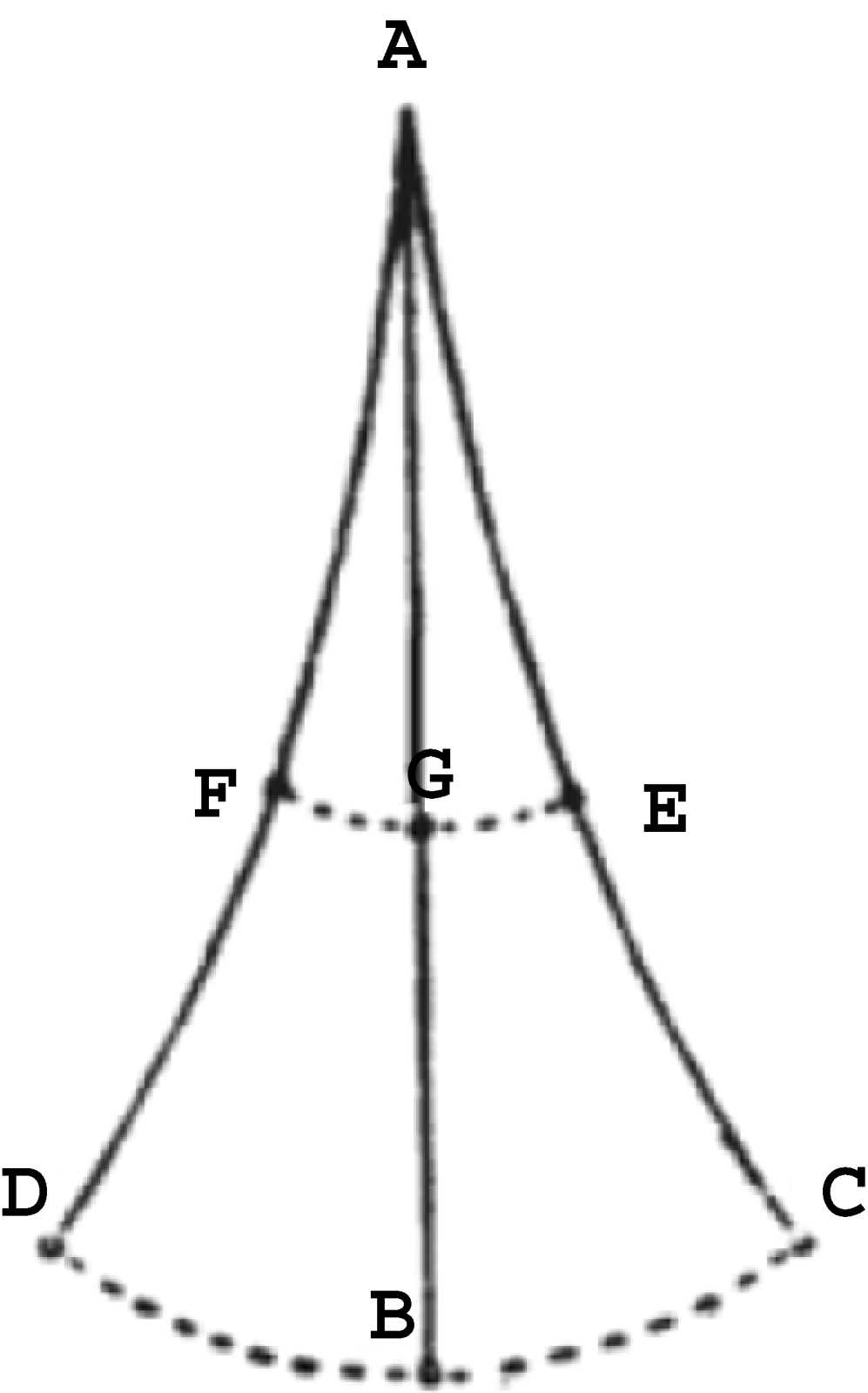
Why a chain? I replicated Galileo's experiments with chain pendulums in order to observe the shape taken by the pendulum while oscillating. The results were astounding – possibly, in my view, the most important finding in the scene of experience. These experiments with chain pendulums revealed the existence of latent modes of oscillation, as they are sometime referred to in the technical literature. A pendulum's latent modes of oscillation are infinite, though only some can be observed. Latent modes of oscillation are well known to structural engineers of the twentieth century. There are infinite possible shapes that a continuous mechanical system, such as, for example, a heavy rope, or a chain, can assume while oscillating. What Galileo shows us (Figure 7) is what structural engineers call the fundamental mode of oscillation, the shape of the oscillation that occurs at the lowest possible frequency. In reality, the motion of the pendulum is always a composite of all possible shapes, though we can normally observe only a few, since those at higher frequencies are more difficult to perceive clearly and distinctly.

The observation of the latent modes of the chain pendulum at last explains why Galileo insists on using pendulums made with thin strings.Footnote ²² Thin strings eliminate the problem of latent modes of oscillation. There is no doubt that Galileo was, from an early stage, well aware of the fantastic display of the latent modes of oscillation. Before further discussion of the implications of this finding, we need to present the latent modes of oscillation more graphically. First of all, I hung brass chain pendulums of different lengths and did what I had been doing with string pendulums, simply removed them from the perpendicular and let them go. If the starting angle is relatively small, the shape the chain pendulum takes is the simple shape of the fundamental mode, exactly like that shown by Galileo. But if the angle increases, more modes start to develop. Videos 22 to 24 (‘The chain pendulum’) show the fantastic behaviour of the latent modes of oscillation. The chain pendulums oscillating at a sufficiently wide angle clearly display the superimposition of a few latent modes, which give the chain pendulum's motion its characteristic, apparently chaotic, serpentine shape.

Table 2 shows approximations of the latent modes of oscillation of a chain pendulum, starting from the lowest frequency. I have calculated the modes with a hundred-mass linear model of the chain pendulum.Footnote ²³ There are exactly one hundred modes for a hundred-mass model. The table shows eight modes, corresponding to the eight lowest frequencies, in order of ascending frequency.

Table 2.

The eight latent modes corresponding to the eight lowest frequencies, in order of ascending frequency, for a hundred-mass linear model of the chain pendulum (the black dots represent some of the masses). Mode number 1 practically matches Galileo's picture. During a real oscillation all the modes contribute, with different weight factors, to the formation of a complex shape

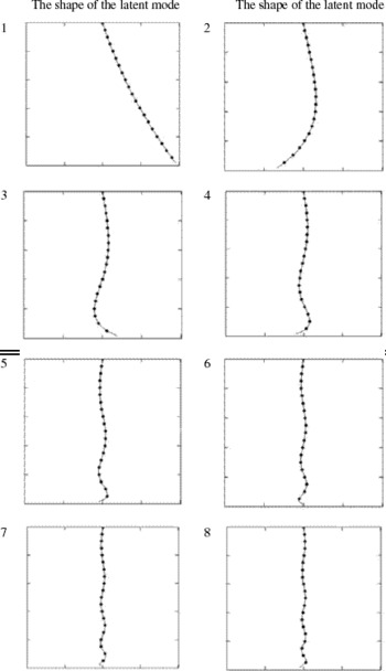
The discovery of the latent modality present in the chain pendulum explains why Galileo otherwise always emphasizes the use of thin strings (which do not show latent modality). It also has further important implications. First, as already noted, the behaviour of the chain pendulum for increasingly wide angles shows correspondingly diminished regularity. It is obvious that the chain pendulum does not have a proper period of oscillation. It is hard to decide what the period of oscillation of the chain pendulum should be. This is because it is difficult to fix the meaning of ‘oscillation’ since the chain constantly assumes different shapes. It appears to have a continuously changing shape. Yet any theoretical use of the pendulum presupposes that a pendulum has by definition a period of oscillation. As all the primary texts suggest, Galileo constantly reiterated that simple pendulums are either isochronous or at least quasi-isochronous.Footnote ²⁴

Second, Galileo chooses to focus on the regularity that the chain pendulum displays for lower angles of oscillation and lower frequencies. There is a tendency in the behaviour of the chain pendulum. The operator controls the unruliness of the pendulum by decreasing the angle of the initial release of the pendulum. Thus the operator learns that regularity tends to manifest itself within the range of small angles of oscillation. Oscillations are observable, somehow, though the operator increasingly wonders about the meaning of oscillation for a chain pendulum. Regularity and oscillation manifest themselves together. I speculate that if Galileo started his pendulum experiment with chain and/or rope pendulums and heavy masses, he would have encountered the unruly latent modality. He would subsequently have decided to go on to experiment with lighter apparatus, such as strings and light masses, in order to control the phenomena of latent modality.

Finally, and most importantly, what would Galileo's reaction have been to the latent modality of the chain pendulum? It is impossible to say exactly when the chain pendulum experiments were really carried out by Galileo, since the only reference to the chain pendulum is given in one passage from the 1632 Dialogue.Footnote ²⁵ But on the assumption commonly accepted by scholars that most experiments would have been done at Padua, we can speculate on the basis of the letter to Guido Ubaldo dal Monte of 29 November 1602. This is a very early Paduan text in which Galileo states something important about the predictive power of mathematical demonstration when put to the test of experience. He argues that, when it comes to matter, the conclusions abstractly demonstrated by the geometer are altered, and that there cannot be science (scienza) of such altered conclusions. The geometer, Galileo concludes, is exempt from the responsibility of dealing with the many alterations introduced by matter in the outcome of the effects predicted by geometrical demonstrations.Footnote ²⁶ Thus I would argue that the 1602 Galileo would have shown little or no concern for the intriguing imperfection of experience. Matter is solely responsible for the unruly modality displayed by the chain pendulum.

Galileo's investigative pathways around the pendulum: (3) experience in the limit

This section deals with two crucial issues: the isochronism of simple pendulums (simple pendulums oscillate at a constant frequency regardless of the oscillations' amplitudes); and the synchronism of pendulums of different materials (simple pendulums, whose bobs are of different materials but whose lengths are the same, oscillate at the same frequency).

Before starting the discussion about the isochronous behaviour of simple pendulums, a question has to be answered concerning Galileo's equipment. This is a question rarely addressed by Galileo scholars. What kind of materials would Galileo have used in his pendulum experiments? We now know that there is a reason why Galileo always proposes pendulums made with thin strings (spaghetti). Thin strings are light, so their latent modality in fact remains latent. Thin string pendulums in fact behave like small masses moving along the circumference of a perfect circle whose radius is the length of the string. The string remains perfectly rectilinear during the oscillations of the pendulum. Thus it is obvious that the masses that Galileo would have preferred are relatively small. Even to a casual experimenter it becomes immediately clear that heavy weights are too dangerous when operating with thin strings, since the speed acquired by the bob of a pendulum four to five braccia long, swinging from a wide angle, is indeed very high. But Galileo almost never tells us anything precise about the weight of the lead balls he uses. There is only one exception. In Two New Sciences he tells us that the lead ball in the experiment of the pendulum twisting around the peg is of one to two ounces (una palla di piombo d' un' oncia o due).Footnote ²⁷ This makes perfect sense. Furthermore, in his time commonly available musket balls would indeed have weighed one or two ounces.Footnote ²⁸

If Galileo used musket balls, or, at any rate, small balls of one or two ounces and thin strings, then his pendulum's patterns of behaviour would have been heavily dependent on the aerodynamic resistance acting on the string and the ball. The literature on Galileo's pendulum experiments consistently misses this important point: light pendulums behave in a way governed by aerodynamic resistance. This is not to say that Galileo never extended his range of operations to pendulums heavier than one or two ounces. Although we lack any textual evidence in this regard, it is likely that a curious experimenter, such as Galileo, would have tried different materials, different sizes and different lengths. In the letter to Guido Ubaldo, for example, Galileo argues that the experience he made was done with two equal bobs, but that it makes no difference if the bobs are different.Footnote ²⁹ The point is that by experimenting with different weights and lengths Galileo would have been exposed to the significant effects of aerodynamic resistance on pendulums. In other words, he would have been exposed to the range of patterns of behaviour that real pendulums display.

A simple pendulum, as we know, is not isochronous (Figure 8). Videos 5 to 7 (‘The isochronism of the pendulum’) show two light pendulums of about ninety-two inches loaded with one-ounce lead balls. The synchronous behaviour of the pendulums is evident. As Galileo would have said, the two pendulums go together. In the third video, the angle of release was slightly wider, so the pendulums start showing some discrepancy. When experimenting with pendulums oscillating along not too wide angles, up to about thirty to thirty-five degrees and in the range of four to five braccia, the whole oscillation can be observed quite easily. The speed of the bob when crossing the vertical is not too high.

Figure 8.

The non-isochronism of the simple pendulum. The curve shows the period of oscillation of a simple pendulum (the time required to complete a whole oscillation) as a function of its length. On the vertical axis, the period is represented in seconds. On the horizontal axis the angle of the swing is represented in degrees, for angles between 0° and 90°. The curve has been calculated for a pendulum length of 2.25 meters. The variability in the period is about one half of one second.

Videos 9 to 12 (‘The discrepancy of the pendulum’) show the change in the visual appearance of the pendulums as the angles of release of the bobs are progressively increased. I call this phenomenon ‘discrepancy’. During my experiments, the best way to get to grips with this gradual change in visual appearance (or at least the way that worked best for me) is to focus observation on the stopping points of the two bobs, the points where the bobs invert their motions. At those instants the bobs have zero speed. At that moment it is easy to ascertain if their motions start again at the same instant, or if they do not arrive at the inverting point at the same instant.Footnote ³⁰

Before discussing the implications of these findings, I need to stress that the results obtained with my apparatus, the phenomena of isochronism and discrepancy, are very robust: they occur over a wide range of the pendulum's parameters. Robustness is difficult to test in practice, since these tests are very time-consuming (and resource-consuming, since one has to find numerous pieces of equipment, such as lead balls of different weights and so on). To test robustness, I repeated a whole set of experiments concerning the discrepancy phenomenon with two-ounce balls. The results, consistent with the one-ounce pendulums, are documented in Videos 13 to 16 (‘The discrepancy of the pendulum 2oz’). Robustness is where the power of computer modelling can be applied. With the pendulum model discussed in the ‘Supporting document’ calibrated on the real data acquired from the real apparatus, I have tested the phenomena of isochronism and discrepancy over a range of plausible parameters. I report one example of the phenomenon of discrepancy, in the form of so-called time histories of the angles of two pendulums. This was obtained with the pendulum model for a pendulum of 1.5 metres, the range of two to three braccia that Galileo talks about in the 1602 letter (Figure 9). The diagram only gives an approximate sense of the phenomenon since it is difficult to visualize the data mentally. In order to form a visual sense of the pendular motion, the reader should observe the animation of the phenomenon in S-Video 2 (‘The pendulum model: discrepancy’). The pendulum model is so accurate that the whole phenomenon could hardly be distinguished from a real case.

Figure 9.

The time histories of the angles of two pendulums obtained with the pendulum model, for a pendulum of 1.5 meters. This is the range of two to three braccia that Galileo discussed in the letter of 1602. On the vertical axis, the amplitudes of the two pendulums are represented in degrees. On the horizontal axis, time is represented in seconds. The two pendulums started from 30° and 10°. The simulation was calculated for two minutes. This diagram only gives an approximate sense of the phenomenon. For a better sense, consult the animation of the phenomenon in S-Video 2 (‘The pendulum model: discrepancy’).

Both in real tests and in simulations with the pendulum model, the phenomena of isochronism and discrepancy appear to be robust over a wide range of parameters. Thanks to the robustness assessed with a computer model, I feel confident in concluding that as he experimented with different pendulums and different angles Galileo could not have missed the gradual change in behaviour from isochronism to discrepancy.

The gradual shift from isochronism to discrepancy challenges any observer of the pendulum. What, in Galileo's view, is the cause of the gradual shift from isochronism to discrepancy? A few preliminary comments are necessary before answering the question.

The two most revealing texts in this regard are the 1602 letter and a passage from Two New Sciences (1638).Footnote ³¹ In these texts, Galileo stresses the fact that he numbered the oscillations of pendulums. It remains unclear whether he actually means complete oscillations back and forth, or rather only half oscillations, from one point of maximum elongation to the other. Direct observation of the isochronism of the pendulums, so Galileo seems to hint, is arduous, but numbering the oscillations or ‘vibrations’ (Galileo uses both words interchangeably) is more secure. It is true that in the 1602 letter to Guido Ubaldo Galileo shows a cavalier attitude, concluding that even without bothering to number the vibrations, Guido Ubaldo could easily ascertain the property of isochronism by simply observing the two pendulums. But his stress on counting oscillations in the passage published in Two New Sciences betrays the fact that he realized that counting was the securest way of ascertaining the fact of the matter about isochronism. Counting, however, has its own serious problems, as will be shown presently.

Most Galileo scholars have strangely neglected Galileo's emphasis on counting, the very claim that Galileo consistently makes. It is a most interesting claim. The numbers of oscillations that Galileo claims he could count seem exorbitant. He speaks of hundreds of oscillations. On the other hand, if he meant half oscillations, as some of his descriptive language sometimes seems to imply, the order of one hundred oscillations is not impossible. In fact, the human eye, as I discovered, has the power to discern accurately even tiny oscillations. At any rate it is easy to count one hundred full oscillations or two hundred half oscillations with pendulums in the range of four to five braccia and masses in the range of one to two ounces. The reader can easily verify this by counting the vibrations while looking at the videos. For example, with the light pendulums used in my tests, it is easy to count more than one hundred full oscillations, without a discrepancy of even one count, for angles up to about seventy degrees, which is more or less the maximum angle I could reliably test with my apparatus. This accords with Galileo's claims that it is indeed possible to do so.Footnote ³²

In addition, I used the pendulum model to test this claim for four- to five-braccia pendulums, swinging from initial amplitudes of eighty and five degrees. Galileo says ‘hundreds’, but allowing for the fact that he may have meant half oscillations, the count of one hundred full oscillations becomes two hundred.Footnote ³³ The results are impressive. It is possible to count up to one hundred full oscillations while observing a stable discrepancy between the two pendulums. I conducted two virtual tests with pendulums of one and two ounces. S-Video 80, ‘5 degrees 1 oz pendulums’, and S-Video 80, ‘5 degrees 2 oz pendulums’, show that one hundred full oscillations are possible without a difference of one count. In the second case, however, the discrepancy increases to almost half of one full oscillation, in which case, if Galileo meant half oscillation, the count would amount to a difference of one.

The discrepancy has one very peculiar characteristic. Since the motions of light pendulums slow down rather quickly because of aerodynamic resistance, after a short time from the start the pendulums enter a region of oscillations where the difference in their periods diminishes. Thus, after accumulating for a while, the discrepancy plateaus and appears to be rather constant over the remaining interval of observation. This, once again, is consistently true over a wide range of parameters. The discrepancy, in other words, does not explode into chaotic patterns of behaviour. It remains clearly visible at a level that seems to be perfectly stable over a long period of observation.

Furthermore, it seems mistaken to count the same number of oscillations for the two pendulums, and assume, as Galileo does, that this is a basis for concluding that all the oscillations are isochronous. Galileo seems well aware of this problem. In the 1602 letter he says that the counts' identity for both pendulums is a sign of isochronism. And in the passage from Two New Sciences, where he draws the same conclusion, he says that the experience of counting makes us certain of isochronism. So experience furnishes at most a sign, or makes us certain of the fact.

We are now in a better position to appreciate the question of the cause of the gradual shift from isochronism to discrepancy. Galileo cannot have failed to confront the isochronism-versus-discrepancy phenomenon. It is all too evident across the whole spectrum of parameters. Yet we are told nothing in the published record and no surviving manuscripts illuminate this issue. Yet why would Galileo otherwise have so consistently emphasized counting rather than direct visual inspection of the phenomenon as the means of ascertaining the facts of the matter? I think that this is because of the gradual shift from isochronism to discrepancy. In the published Dialogo text where Galileo dispenses with counting, he hastens to emphasize that experience shows that the pendulums are isochronous, or if not perfectly isochronous, then at least quasi-isochronous (again, without using precisely these words). He does not say that experience shows perfectly isochronous pendulums.Footnote ³⁴

Eventually Galileo must have asked himself about the cause of the gradual shift from isochronism to discrepancy. For the early Galileo, the implications of this gradual shift were far more serious than the imperfection of the pendulum experience. We need to go back to the De motu writings to understand why. In the De motu writings, Galileo vehemently opposes the Aristotelian theory of rest at the point of inversion. The problem was addressed by Galileo under the heading of ‘point of reflection’ (punctum reflexionis). Galileo opposes the Aristotelian view that, in order for motion to be inverted, such as, for example, in the case of a stone thrown upwards, which will invert its upward motion before starting its downward motion, a rest occurs at the point of inversion.Footnote ³⁵ Galileo reconstructs Aristotle's main line of argument as follows:

Galileo's counterargument to the theory of rest at the point of inversion is based on five distinct independent strategies. We need not dwell on the first four, since the fifth, the most elaborate, is that whose relevance for the young Galileo's theory of motion was now at stake in the face of new empirical evidence from the pendulum discrepancy. I will only provide the gist of the fifth strategy. Two assumptions are first introduced by Galileo.Footnote ³⁷ First, mobiles will only rest outside their own place when the virtue preventing their descent is equal to the gravity of the mobiles pushing them downwards. Second, the same mobile can be sustained in the same place by equal virtues for equal intervals of time. Now, if a stone rests for some time at the point of inversion, then, for the same duration, there will be equality of impelling virtue and resisting gravity. But this is impossible since, Galileo argues, it has already been shown in another chapter of De motu that the impelling virtue must diminish continuously. He then moves on to reframe the argument in the form of a stronger reductio ad absurdum. We need not follow Galileo through the details of the proof. What is at stake is clear. It is the theory of the impelling virtue, the theory of impetus. Let us now return to the discrepancy.

It might be appealing to explain the cause of the gradual shift from isochronism to discrepancy by saying that at the point of inversion the bobs will indeed rest for a short while. But one could take a step further. On the assumption that the wider the oscillation the rather longer the time of rest at the point of inversion, one could explain why the discrepancy seems to accumulate faster at the beginning of the phenomenon before levelling out and eventually becoming virtually constant. No better experience could confirm the cause of the gradual shift from isochronism to discrepancy than observation of the discrepancy becoming increasingly evident as the operator moves one pendulum ever further from the vertical. Aristotle's theory of the rest at the point of reflection would be correct after all.

I speculate that Galileo did not reject isochronism and remained steadfast in rejecting Aristotle's theory of the rest at the point of reflection because in De motu he stated that ‘experience does not teach us the causes’.Footnote ³⁸ The norm that ‘experience does not teach us the causes’, which Galileo followed at this early stage, became a stabilizing factor in Galileo's search for a mathematical–mechanical theory of isochronism. Galileo's commitment to that norm thwarted the threat posed by the discrepancy and by the lure of explaining the discrepancy via Aristotle's theory of rest at the point of reflection. The isochronism-versus-discrepancy phenomenon was destabilizing not only for a mathematical–mechanical theory of isochronism, but for the whole De motu, which was entirely based on the theory of impetus as the explanatory principle of the impossibility of rest at the point of inversion.

Experience with pendulums offered the early Galileo two opportunities. One was the possibility of explaining the regularity of isochronism, which must have appealed to Galileo the mathematician. The second was the possibility of explaining the gradual shift from isochronism to discrepancy with the abhorred theory of rest at the point of inversion, possibly rejecting isochronism altogether. The second possibility must have appealed to Galileo the natural philosopher. Paradoxically, a norm regulating the philosopher's quest for causes aided and abetted the mathematician in the pursuit of proof.

In a text published in Two New Sciences, Galileo reports pendulum experiments with cork and lead balls. Galileo claims that two pendulums, one made with a cork ball, and another with a lead ball one hundred times heavier than the cork ball,

Galileo's wording is so carefully judged that it almost defies translation. Galileo seems to claim that what happens is the reiteration of one hundred comings and goings (reiterando ben cento volte per lor medesime le andate e le tornate), so that experience shows the two bobs going at the same pace for a hundred or even a thousand vibrations. Clearly the claim of a thousand vibrations is no more than a conclusion based on reasoning, since Galileo has just claimed that what happens is a hundred comings and goings. He also claims that the heavy ball is never ahead of time for a moment. Further, the disclaimer at the end of the passage stresses that this experiment is not supposed to show isochronism. Galileo specifies that ‘on the other hand, when the arcs traversed by the cork were no more than five or six degrees and those of the lead no more than fifty or sixty degrees, they are traversed under the same times’ (anzi quando gli archi passati dal sughero non fusser più che di cinque o sei gradi, e quei del piombo di cinquanta o sessanta, son eglin passati sotto i medesimi tempi).

Galileo's claim about lead and cork pendulums concerns the synchronism of pendulums with bobs of different materials but the same lengths. In another paper, I have explored the context of Galileo's claim – the theory that all bodies fall at the same speed regardless of weight and material.Footnote ⁴⁰ In what follows, I will discuss the findings of my experiments with lead and cork pendulums.

The most serious problem is Galileo's assertion that the lead ball is one hundred times heavier than the cork ball. In fact, cork's specific weight is so much smaller than lead's that for a lead ball to be one hundred times heavier than a cork ball, either the cork ball must be very light or the lead ball must be very heavy. Both cases present problems. A cork ball that is too light will not oscillate long enough, while a lead ball that is too heavy is hard to reconcile with Galileo's indication that he is still using thin strings (due sottili spaghetti). I have been able to count about fifty full oscillations with balls that weigh approximately in the ratio given by Galileo.

Videos 17 and 18 (‘Cork and lead’) show tests made with balls in a ratio close but not exactly equal to that of one to a hundred: cork ball=8 grams, lead ball=670 grams. In Videos 19 and 20 (‘Cork and lead’) I changed the ratio so that: cork ball=18 grams, lead ball=670 grams; and cork ball=7 grams, lead ball=670 grams. Video 21 (‘Cork and lead’) shows that there is no interference between the pendulums. The lengths of the two pendulums were about ninety-four inches. It is possible that the ratio indicated by Galileo is not realistic. But it is impossible to rule out the possibility that Galileo could operate with balls in exactly that ratio. We are left with an uncertainty.Footnote ⁴¹ The pendulums show a gradual shift from synchronism to discrepancy, with the cork ball moving ahead. This is due to the fact that, because it decelerates rapidly, the cork ball enters the region of small oscillations, thus starting to move ahead of the lead ball.

So, once again, experience issues a challenge to the experimenter, the transition from passo egualissimo to discrepancy. Galileo is on safe ground while claiming that neither in a hundred nor a thousand vibrations is the heavy ball ahead of time. In fact the opposite happens with the gradual emergence of the discrepancy. Do the balls go at the same pace (camminano con passo egualissimo)? For some time they do. Since Galileo is careful not to say from what angle the balls are supposed to be released, it is quite possible, for small oscillations, to see the balls go con passo egualissimo for some time.

If such experiments were carried out early on, as the 1604 letter seems to suggest when Galileo claims that it would not matter if the bobs were of different weights, then we can ask what Galileo would have made of these results in the framework of his early De motu writings. According to the De motu Archimedean framework, specifically heavier bodies will move faster in fluid media than specifically lighter bodies.Footnote ⁴² In concluding De motu Galileo candidly admits that experience contradicts the proportions of motions calculated on the basis of the Archimedean framework.Footnote ⁴³ This claim by Galileo has thus far remained a mystery. To what experiments does he allude?Footnote ⁴⁴

I hypothesize that these are the experiments with lead and cork pendulums. They seem to suggest that specifically lighter bodies will move faster than specifically heavier bodies. How could a mighty lead ball lag behind the cork ball? Unfortunately the Archimedean framework is silent about the resistive role of the medium. For Aristotle and for the Aristotelians attacked by Galileo in De motu, the medium is the cause of, not a hindrance to, the motion of projectiles. If we suspend the belief that media resist motion, we can see that the latter question must have been deeply troubling for the young Galileo. Could the medium be more effective in pushing the cork ball than the lead ball?

A cork ball starts moving ahead of a lead ball. What is the cause of such a bizarre phenomenon? Might a new theory of the resistance exerted by the medium be brought to bear on the Archimedean framework, so as to prevent the latter from collapsing in the face of negative evidence from the cork and lead pendulums? The cork and lead pendulums somehow seem to teach us something about fluid media that is missing in both the Aristotelian and Archimedean frameworks. Fluid media can resist motion. They can be the cause of resistance. Does experience tell us more about causes than we might have suspected, contrary to the De motu's statement that ‘experience does not teach causes’? Here we see the challenges of pendulum behaviour behind Galileo's crucial transition from the De motu writings to a more mature theory of motion.

Pendulums show isochronism, synchronism and discrepancy along a continuum of patterns of behaviour. There is no such thing, then, as the pendulum experience. The pendulum experience is an experience in the limit, in the sense that isochronism and synchronism tend to manifest themselves increasingly well as the parameters that control the outcome of the experiment tend to certain values. This is also true of latent modality. Latent modality tends to disappear as the parameters that control it tend to certain values.

Galileo's investigative pathways around the pendulum: (4) artefacts restrained

Artefacts may be unpredictable in interesting ways. Latent modality was discovered in the chain pendulum. In the gallows-like apparatus I built, I discovered ‘coupling’, a phenomenon present from the very start. Coupling is an interference of some sort between the two pendulums. Coupled pendulums may mislead the observer by tuning themselves to each other, for example, or by driving each other. Coupling, therefore, may determine quite bizarre oscillatory patterns. It is a fascinating phenomenon that may affect all pendulum experiments. So far as I know, it has never been investigated in the literature concerning Galileo's experiments. This section briefly discusses coupling and its consequences for pendulum experiments, and argues that we can reasonably exclude any serious impact on Galileo's experiments of coupling.

There are at least two forms of coupling, mechanical and aerodynamic. I made sure that coupling did not affect my experiments by checking that the two pendulums did not interfere with each other. This is why, as noted above, I controlled the outcome of my experiments by always checking, in a preliminary test, that while one pendulum was going the other stayed at rest. However, a coupling phenomenon was clearly observable in the case of the very heavy lead ball used to test the 1:100 ratio in the cork and lead pendulums. Its origin is mechanical. I will focus firstly on mechanical coupling, then briefly on aerodynamic coupling.

Galileo tells us almost nothing of the set-up of his pendulums. It is perfectly possible that he simply hung pendulums next to each other, from the ceiling of his workshop or bedroom, or on a wall, as shown in the diagram accompanying the 1602 letter to Guido Ubaldo.Footnote ⁴⁵ I have imagined the gallows-like structure on the basis of two considerations. First, it is a structure that allows for the two pendulums to be seen in front of each other, thus also allowing for a better observation of their relative motions. Second, I was inspired by a similar structure later devised by the Galilean experimenters at the Accademia del Cimento in Florence. The horizontal arm of the structure has some flexibility that allows the arm to bend under the forces exerted by the oscillating masses. If the masses are modest then so are the forces, but if the masses are greater then the forces might be considerable. However, the flexibility can be controlled by connecting the horizontal arm with barely extensible or inextensible cables to fixed points on walls. This is how I practically eliminated the unwanted flexibility – ‘practically’ because in the case of the heavy lead ball I was unable to eliminate all the flexibility. This residual flexibility explains why coupling was observable with the heavy lead ball. The heavy lead ball was able to drive the light cork ball for dozens of oscillations through mechanical coupling induced in the flexible structure, as shown in Video 26 (‘Cork lead 4lb interference’) and Videos 27 to 29 (‘Cork lead 4lb discrepancy’).

Yet in these circumstances, under the regular alternating pull of the heavy ball, the horizontal arm quite visibly and regularly bends to right and left through around two or three inches at the farthest point from the joint. If Galileo ever used a structure like that I have reinvented, and if this kind of mechanical coupling were observable when he experimented, he must have realized something in the set-up was seriously flawed and that a corrective was needed. Thus I do not believe that his accounts, particularly of the cork and lead experiments, can be explained away in terms of significant mechanical coupling phenomena of which he might have been unaware. Can we exclude the possibility that mechanical coupling was not affecting Galileo's pendulums under all possible circumstances, even when operating with small masses?

While it is impossible absolutely to exclude mechanical coupling, we can at least use computer models to investigate the case of isochronism for small masses such as the one- or two-ounce lead balls that I think Galileo used. Consider the imaginary set-up represented in Figure 10. Suppose that Galileo hung his pendulums from a structure that, unknown to him, at least initially, allowed for some flexibility. Might he have been misled by mechanical coupling into the belief that two pendulums were perfectly isochronous? In other words, might structural flexibility subtly and viciously couple the pendulums in such a way as to make them oscillate in tune with each other?

Figure 10.

Above: A simplified sketch of the structure, with a light horizontal arm rigidly attached to a stronger vertical frame. Mechanical coupling is possible if the horizontal arm of the structure bends. In this case, the points at which the strings are attached will move accordingly. Below: An imaginary structure where a flexible horizontal arm is connected to a sturdier, fixed beam above.

Consider Figure 11. A simulation was carried out for three minutes with pendulums of one-ounce masses and strings of ninety-two inches, to observe an example of the highly complex patterns of behaviour that may develop because of coupling. The two pendulums drive each other. The pendulum that is started from the higher angle, which has more energy, initially pushes the other. But the latter responds because of the interaction through the structure and slows the first pendulum. The pattern at one point shows that the phenomenon is reversed. I am convinced that this strange pattern of behaviour is too evidently an artefact of the mechanical structure to be mistaken as genuine, even by naive observers. The horizontal arm's ends alternately move back and forth with amplitudes up to ±2 cm, a fact which should alert any observer. So we can confidently exclude the possibility that such odd examples might have been mistaken for anything more than an exceptional result due to the particular set-up.

Figure 11.

Above: a spectacular yet bizarre case of coupling. On the vertical axis angles are represented in degrees, while on the horizontal axis time is represented in seconds. The pendulums drive each other while developing a highly complex pattern of behaviour. One mass was started from 50° and one mass from 5°. The pendulum starting from the higher angle ‘pushes’ the other pendulum, which in turn responds by amplifying its oscillation while slowing the other. The pattern is then almost reversed. Below: a much more ambiguous and perplexing pattern. After an initial phase of energetic interaction, the two pendulums tune to each other so well that they continue oscillating as if perfectly superimposed on each other.

However, there are more subtle possibilities. Consider now Figure 11. Another simulation was carried out for three minutes, again with pendulums of one-ounce masses and strings of ninety-two inches. The result is subtly different. After an initial phase of energetic interaction the two pendulums tune to each other so well that they go on oscillating as if they were perfectly superimposed on each other. However, even in this more delicate case, the visible motion of the ends of the horizontal arm should alert the observer to the possibility that something in the mechanical structure of the arrangement is affecting the oscillations of the pendulums.

How do these results translate into dynamic visual appearances? We can form an idea of the real dynamics of the phenomenon of coupling by animating the numerical results obtained with the coupled pendulums. S-Video ‘Coupling 1’ and S-Video ‘Coupling 2’ animate the two patterns of behaviour diagrammatically presented in Figure 11. Only the pendulums are shown, even though, in reality, in the scene of experience, the oscillations would appear in their natural setting with the horizontal arm flapping back and forth.

Consider now the possibility of aerodynamic coupling. If the pendulums are placed very close to each other in an arrangement such as, for instance, that shown in Figure 10, or when simply hanging from a ceiling, the question arises whether aerodynamic forces especially generated by the strings could make the two pendulums interfere with each other. First, the observations made with one pendulum at rest and the other oscillating again confirm that such a phenomenon was not affecting the results in my experiments. Moreover, it is somewhat difficult to place the pendulums very close to each other, because their planes of oscillation often tend to rotate in one way or another. The danger of collisions tells against the idea of such an arrangement. In conclusion, we can exclude the possibility that coupling phenomena might have consistently vitiated the results that Galileo obtained with pendulums.

Conclusion

I thank an anonymous referee for making these comments on a previous draft of this paper. Though it is unclear whether Galileo himself held that a companion should help out or witness the experiment, I like to think that Galileo would have welcomed computer modelling in the discussion of the pendulum. As with mathematical demonstrations, and against the Aristotelian meditator Simplicio, Galileo–Salviati famously claims in the celebrated Dialogo that whenever mathematical proofs are available we should gladly make use of them. The technology of computer modelling, like the technology of mathematical proof, is only an extension of our analytical powers, not a substitute for theory and real experiment. But if it is affordable it should be used. The sensual and the bodily are essential for producing as well as witnessing, and calibrating, computer models of irregularities and discrepancies, even though owing to current division of labour the modeller's body may not be involved in the actual making of the computer itself.

Galileo's pendulum was an open-ended artefact. Its elusive features challenged the norms that presided over the tentative construction of a new methodology for science. However, the possibility of destabilization also acted as an invitation to explore new investigative pathways.Footnote ⁴⁶ Galileo's detour around the pendulum was path-breaking. It was a risky enterprise. The element of risk is inherent in Galileo's new science. Galileo's new science emerged from a willingness to negotiate and trade theoretical norms for stubborn facts of experience, and sometimes, no doubt, the other way round, to the consequent discomfort of later scholars. Praxis and theory were placed on an equal, unstable footing. In this paper, I have emphasized a phenomenological reading of texts in the light of lived-through experiment by letting body and perception take centre stage.