


1. Introduction
In classical logic, propositions are ascribed to exactly one truth value: true or false. While this bivalent framework has been indispensable in numerous mathematical and logical applications, the inherent simplicity and rigidity may fall short in capturing the intricacies present in real-world scenarios. For instance, in Software Engineering, it is common to encounter application scenarios where requirements either reinforce or contradict each other. One such scenario comes from current practice in quantum computation in the context of NISQ (Noisy Intermediate-Scale Quantum) technology (Preskill Reference Preskill2018) in which levels of decoherence of quantum memory need to be articulated with the length of the circuits to assess program quality. Similar challenges emerge in AI applications and data engineering.
The foundation of our work lies in a recent paper (Cruz et al. Reference Cruz, Madeira, Barbosa, Indrzejczak and Zawidzki2022a), where the authors introduced a weighted transition systems that records, for each transition, a pair of weights, a positive and a negative one. Informally, the positive weight captures the degree of effectiveness (‘presence’), and the negative weight captures the degree of impossibility (‘absence’) of a transition. This allows models to capture both vagueness, whenever both weights sum less than 1, as usual for example, in fuzzy systems, and inconsistency, when their sum exceeds 1. This last feature motivates the qualifier paraconsistent borrowed from the work on paraconsistent logic (Jaśkowski Reference Jaśkowski1969; da Costa et al. Reference da Costa, Krause, Bueno and Jacquette2007), which accommodates inconsistency in a controlled way, treating inconsistent information as potentially informative. Such logics were originally developed in Latin America in the decades of 1950 and 1960, primarily through the influential works of F. Asenjo and Newton da Costa. Quickly, however, paraconsistent logic attracted attention in the international community and the original scope of mathematical applications broadened out as witnessed in a well-known book emphasizing the engineering potential of paraconsistency (Akama Reference Akama2016). A number of other applications have emerged to themes from robotics, quantum mechanics and quantum information theory in works by Abe et al. (Reference Abe, Torres, Lambert-Torres, da Silva Filho, Martins, Lambert-Torres, Abe, da Silva Filho and Martins2007), Chiara and Giuntini (Reference Chiara and Giuntini2000), Agudelo and Carnielli (Reference Agudelo and Carnielli2010) and da Costa and Krause (Reference da Costa and Krause2014).
Paraconsistent transition structures and their composition were further studied in the preliminary conference communication (Cruz et al. Reference Cruz, Madeira, Barbosa, Nantes-Sobrinho and Fontaine2022b) that this paper extends. The research program in Cruz et al. (Reference Cruz, Madeira, Barbosa, Nantes-Sobrinho and Fontaine2022b) continued here in two directions. First a suitable notion of morphism for paraconsistent labeled transition systems (PLTS) was introduced leading to the definition of the corresponding category and its algebra. Then, notions of trace for PLTS were discussed, as well as, notions of crisp (i.e. bivalent) simulation and bisimulation to relate two paraconsistent transition systems.
This paper starts by revising this work, namely lifting the residuated structure underlying the (parametric) domain of weights to the twisted structure which enables joint computation of positive and negative weights. We adopt the framework outlined in Bou et al. (Reference Bou, Esteva, Godo and Rodríguez2009) and focus on many-valued (paraconsistent) modal logics defined over commutative integral residuated lattices over a set
 $A$
of possible truth values. The motivation behind these systems is to combine modal and graded reasoning, with existing research on many-valued logic addressing problems related to decidability, complexity (Caicedo et al. Reference Caicedo, Metcalfe, Rodríguez and Rogger2017), and axiomatizability of a (many-valued) dynamic logic (Madeira et al. Reference Madeira, Neves and Martins2016). Further contributions such as (Badia et al. Reference Badia, Caicedo and Noguera2023) involve investigating frame definability in finitely valued modal logics and Marti and Metcalfe (Reference Marti, Metcalfe, Goré, Kooi and Kurucz2014) delves into the expressivity of modal languages in a many-valued setting. Subsequent work in Badia and Olkhovikov (Reference Badia and Olkhovikov2020) demonstrated that no compact extension of these many-valued logic, displays both the Tarski Union Property and strong invariance for the proposed notion of crisp bisimulation introduced in Marti and Metcalfe (Reference Marti, Metcalfe, Goré, Kooi and Kurucz2014).
Some of the previously cited works (Marti and Metcalfe Reference Marti, Metcalfe, Goré, Kooi and Kurucz2014; Badia et al. Reference Badia, Caicedo and Noguera2023) concentrate on crisp many-valued logics, where accessibility is a binary relation and proposition valuation is many-valued, parametric to a residuated lattice
 $A$
. While other works (Caicedo and Rodríguez Reference Caicedo and Rodríguez2015; Jain et al. Reference Jain, Madeira, Martins, Felty and Marcos2019) delve into fuzzy Kripke models, where both propositions and the accessibility relation are many-valued, taking values in the standard Gödel algebra
 $[0,1]$
. Our approach aims to combine these perspectives by working with models that are parametric to a residuated lattice
 $A$
, where the accessibility and valuation relation are many-valued, taking values in
 $A\times A$
. We believe that this approach not only admits different instances to better suit each modeling problem at hand but also provides a nuanced perspective, allowing transitions and propositions to represent consistent, vague, or inconsistent information.
This paper extends (Cruz et al. Reference Cruz, Madeira, Barbosa, Nantes-Sobrinho and Fontaine2022b) with three main contributions:
-
(1) A notion of graded simulation and bisimulation, which enables comparing PLTS in a (formal) paraconsistent way;
-
(2) A modal (minimal) logic over the corresponding Kripke models, in which, in the tradition of so-called Hennessy-Milner logics, modalities are indexed by transition labels, or actions;
-
(3) A number of results on modal preservation by both crisp and graded simulations and bisimulations.
Alternatively to the concept of simulation or bisimulation as a crisp relation, typically used in many-valued logics (Marti and Metcalfe Reference Marti, Metcalfe, Goré, Kooi and Kurucz2014; Jain et al. Reference Jain, Madeira, Martins, Felty and Marcos2019; Cruz et al. Reference Cruz, Madeira, Barbosa, Nantes-Sobrinho and Fontaine2022b), we study the concept of simulation and bisimulation as paraconsistent relations themselves. That is, a relation associating to each pair of states a pair of weights witnessing, respectively, the level of confidence or rejection on such a relationship. This leads to a less strict notion of simulation and bisimulation, aligning with the inherent uncertainty and inconsistencies possibly present in PLTS. Our work draws inspiration from Nguyen (Reference Nguyen2022), where a logical characterization of fuzzy bisimulations in fuzzy modal logics is given. Thus, we extend this approach exploring logical characterizations of paraconsistent bisimulation in a paraconsistent modal logic over a general residuated lattice.
Preliminary results on classical soundness and the introduction of graded soundness for paraconsistent Kripke models are presented in § 5.2. In contrast to classical soundness, graded soundness allows for premises and conclusions that may involve vagueness or contradiction. A similar motivation can be found in Caicedo and Rodríguez (Reference Caicedo and Rodríguez2010), where the authors consider a many-valued version of Kripke semantics in which both the propositions, denoted by function
 $e$
, and accessibility relations, denoted by
 $S$
, are infinitely many-valued in the standard Gödel algebra
 $[0,1]$
. For a Gödel-Kripke model
 $GK=\langle W, S, e \rangle$
where
 $W$
is a set of worlds, the authors define set
 $e(x,T) \,=\, \{e(x,\varphi )\,:\,\varphi \in T\}$
which corresponds to a collection of valuations, that is, values in
 $[0,1]$
. A graded notion of logical consequence arises naturally as
 \begin{equation*}T \models _{\leq GK} \varphi \; \text{ iff for any $GK$-model $M$ and any world $x$ in $M$, } \text{inf}\, e(x,T)\,\leq \, e(x,\varphi )\end{equation*}
Then it is proved soundness for the
 $\square$
-fragment and
 $\diamond$
-fragment. Soundness is stated as
 $T \vdash _{\mathcal{G}_\square } \varphi$
implies
 $T \models _{\leq GK} \varphi$
, where
 $\mathcal{G}_\square$
is the
 $\square$
-fragment. Our approach to defining graded soundness for paraconsistent models is similar. However, the main difference lies in studying theories where the classical notion of logical consequence is not equivalent to the graded one.
This work is part of a broader research agenda, of which we highlight references on specification theory and the stepwise implementation process (Sannella Reference Sannella2012) applied to paraconsistent transition systems and their corresponding processes (Cunha et al. Reference Cunha, Madeira, Barbosa, David and Sun2023a,b). An application example of these systems to optimisation of quantum circuits, briefly mentioned in Cruz et al. (Reference Cruz, Madeira, Barbosa, Nantes-Sobrinho and Fontaine2022b), is further discussed in reference Barbosa and Madeira (Reference Barbosa, Madeira, Chiba, Cong and Boix2023).
Paper Structure. Section 2 revisits the concept of a PLTS and characterizes the twisted structure for the joint computation of positive and negative weights. The whole construction is parametric on a residuated lattice from which weights are taken. The compositional construction of (pointed) PLTS are characterized in § 3 by exploring the relevant category, following G. Winskel and M. Nielsen’s ‘recipe’ (Winskel and Nielsen Reference Winskel, Nielsen, Abramsky, Gabbay and Maibaum1995). In § 4, PTLS are extended to (paraconsistent) Kripke models over which notions of crisp and graded simulation and bisimulation are studied. A modal logic for paraconsistent transition structures is introduced in § 5, alongside preliminary results on soundness and modal preservation for crisp and graded simulation and bisimulation. Finally, in § 6, we explore possible applications of PLTS. Section 7 concludes and points out a number of future research directions.
2. Paraconsistent Labelled Transition Systems
In line with the work documented in Bou et al. (Reference Bou, Esteva, Godo and Rodríguez2009), our constructions are parametric on a residuated lattice over a set
 $A$
of possible truth values, which in the classical modal logic corresponds to a Boolean algebra. Our work extends this framework to the paraconsistent case, introducing the concept of a paraconsistent transition system where transitions are represented by pairs of weights
 $(a, b) \in A \times A$
. We further introduce the notion of an
 $\boldsymbol{A}$
-twisted algebra to manipulate pairs of weights, laying the foundation for the subsequent sections.
Formally, a paraconsistent labeled transition system (PLTS) incorporates two accessibility relations, classified as positive and negative, respectively, which characterize each transition in opposite ways: one represents the evidence of its presence and other the evidence of its absence. Both relations are weighted by elements of a residuated lattice
 $\boldsymbol{A} = \langle A, \land ,\lor ,\odot ,\to ,\text{1},\text{0}\rangle$
, where,
 $\langle A, \land ,\lor ,\text{1},\text{0}\rangle$
is a lattice,
 $\langle A,\odot , 1\rangle$
is a monoid, and operation
 $\odot$
is the left adjoint to
 $\to$
, its residuum, that is for all
 $a,b,c\in A$
,
 \begin{equation*}a\odot b\leq c \; \text{ iff }\; b\leq a\to c\end{equation*}
We will focus on a particular class of complete residuated lattices that are bounded by a maximal
 $1$
and a minimal element
 $0$
, respectively, and where lattice meet (
 $\land$
) and monoidal composition (
 $\odot$
) coincide. As these two operators coincide, we will henceforth omit one when working with the residuated lattices. Consequently, the adjunction above can be rephrased as
 \begin{equation} a \land b \leq c \; \text{ iff } \; b \leq \, a \to c \end{equation}
Furthermore, a pre-linearity condition is enforced
 \begin{equation} (a \to b) \, \lor \, (b \to a) \,=\, 1 \end{equation}
A residuated lattice obeying pre-linearity is known as a MTL-algebra (Esteva and Godo Reference Esteva and Godo2001). With a slight abuse of nomenclature, the designation iMTL-algebra, from integral MTL-algebra, will be used in the sequel for the class of semantic structures considered, i.e., complete, prelinear, residuated lattices in which
 $\land$
and
 $\odot$
coincide.
The Gödel algebra
 $G=\langle [0,1], \text{min}, \text{max}, \text{min}, \to ,1,0\rangle$
is an example of such a structure that will be used in the sequel. Operators
 $\text{max}$
and
 $\text{min}$
retain the usual definitions, whereas implication is given by
 \begin{equation*} a \to b = \begin{cases} 1, \text{ if } a \leq b \\ b, \text{ otherwise } \end{cases}\end{equation*}
The following Lemma builds upon [Nguyen (Reference Nguyen2022), Lemma 2.1] to introduce a number of properties of these structures that will be useful in the paper. Since most of the assertions of this lemma are well known and their proofs straightforward, we omit the proof here and refer the reader instead to Appendix A for the proofs of Properties (12), (13), (14), and (16). The remaining properties are proved in Nguyen (Reference Nguyen2022).
Lemma 1.
Let
 $\boldsymbol{A} = \langle A, \land ,\lor , ,\to ,\text{1},\text{0}\rangle$
be an iMTL-algebra over a nonempty set
 $A$
. The following properties hold, for any
 $a,\,a', \, b, \, b',\,c\, \in A$
 \begin{align} &\qquad\qquad a \leq a' \text{ iff } (a \rightarrow a')=1 \end{align}
 \begin{align} & a \leq a' \text{ and } b \leq b' \text{ implies } a \land b \leq a'\land b' \end{align}
 \begin{align} & a' \leq a \text{ and } b \leq b' \text{ implies } a \to b \leq a' \to b' \end{align}
 \begin{align} & (a \leftrightarrow a') \land (b \leftrightarrow b') \, \leq \, (a \land b) \leftrightarrow (a' \land b') \end{align}
 \begin{align} & (a \leftrightarrow a') \land (b \leftrightarrow b') \, \leq \, (a \lor b) \leftrightarrow (a' \lor b') \end{align}
 \begin{align} &\qquad\quad a \to (b \to c) \, = \, b \to (a \to c) \end{align}
 \begin{align} &\qquad\quad a \to (b \to c) \, = \, (a \land b) \to c \end{align}
 \begin{align} &\qquad a \land (b \lor b') \, =\, (a \land b) \lor (a \land b') \end{align}
 \begin{align} &\qquad a \lor (b \land b') \, =\, (a \lor b) \land (a \lor b') \end{align}
 \begin{align} &\qquad\qquad\quad a \land (a \to c) \, \leq \, c \end{align}
 \begin{align} &\qquad (a \to c) \land (b \to c) \, = \, (a \lor b) \to c \end{align}
 \begin{align} &\qquad (a \to b) \land (a \to c) \, = \, a \to (b \land c) \end{align}
 \begin{align} &\qquad\quad a \land (b \to c) \, \leq \, (a \to b) \to c \end{align}
 \begin{align} &\qquad\quad a \land (b \to c) \, \leq \,b \to ( a \land c) \end{align}
The following definition introduces the paper’s basic semantic structure, which is to a large extent, independent of the particular residuated lattice chosen.
Definition 1.
A paraconsistent labeled transition system (PLTS) over a iMTL-algebra
 $\boldsymbol{A}$
, and a set of atomic actions
 $\textrm{Act}$
, is a structure
 $\langle W, R \rangle$
where,
-
•
 $W$
is a non-empty set of states
-
•
$R= (R_{a} \colon W \times W \rightarrow A \times A)_{a \,\in \, \textrm{Act}}$
is an
$\textrm{Act}$
-indexed family of functions. Given any pair of states
$(w_1,w_2) \in W \times W$
and an atomic action
$a \in \textrm{Act}$
, relation
$R_a$
assigns a pair
$(\alpha , \beta ) \in A \times A$
such that
$\alpha$
weights the evidence of the transition from
$w_1$
to
$w_2$
occurring through action
$a$
and
$\beta$
weights the evidence of the transition being absent.






For any pair of weights
 $\omega = (\alpha , \beta ) \in A \times A$
,
 $\omega ^+$
denotes
 $\alpha$
, referred to as the positive weight, and
 $\omega ^-$
denotes
 $\beta$
, referred to as the negative weight.
Example 1.
A PLTS over the set
 $\{a,b\}$
of atomic actions, taking weights from Gödel algebra
 $G$
is depicted below
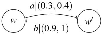
Note that
 $R_a(w,w')$
represents vague information, because the sum of the positive and negative weights for the corresponding transition is less than 1. On the other hand,
 $R_b(w',w)$
represents inconsistent information.
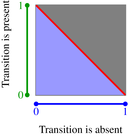
Actually, the road from vague to inconsistent transitions is represented in Figure 1 which depicts all pairs of weights
 $(\alpha , \beta ) \in [0,1] \times [0,1]$
in a Gödel algebra.
The vagueness-inconsistency square.

These pairs of weights jointly express different behaviors:
-
• inconsistency, when the positive and negative weights are contradictory, that is, they sum to some value greater then
$1$
; this corresponds to the upper triangle in Figure 1, filled in grey. -
• vagueness, when the sum is less than
$1$
, corresponding to the lower, periwinkle triangle in Figure 1. -
• consistency, when the sum is exactly
$1$
, which means that the measures of the factors enforcing or preventing a transition are complementary, corresponding to the red line in Figure 1.


This discussion can be lifted to arbitrary iMTL-algebras over
 $A$
through the introduction of a metric space over
 $A^2$
, as proposed in our previous work (Cruz et al. Reference Cruz, Madeira, Barbosa, Indrzejczak and Zawidzki2022a).
Jointly operating with pairs of (positive and negative) weights is essential for defining a (modal) logic over PLTS. The main conceptual tool for this is the notion of a twisted algebra (Kracht Reference Kracht1998).
Definition 2.
Given an iMTL-algebra
 $\boldsymbol{A}\,=\,\langle A, \land , \lor ,1,0,\to \rangle$
a
 $\boldsymbol{A}$
-twisted algebra
 \begin{equation*}\mathcal{A}\,=\,\langle A \times A, \mathrel {\substack {\land \\ \land }} , \mathrel {\substack {\lor \\ \lor }} ,\Rightarrow , \mathbin {/\mkern -6mu/} \rangle \end{equation*}
is defined as follows:
-
•
$(\alpha ,\beta ) \mathrel {\substack {\land \\ \land }} (\alpha ',\beta ') = (\alpha \land \alpha ', \beta \lor \beta ')$
-
•
$(\alpha ,\beta ) \mathrel {\substack {\lor \\ \lor }} (\alpha ',\beta ') = (\alpha \lor \alpha ', \beta \land \beta ')$
-
•
$(\alpha ,\beta ) \Rightarrow (\alpha ',\beta ') = ((\alpha \to \alpha ') \land (\beta '\to \beta ), \alpha \land \beta ')$
-
•
$\mathbin {/\mkern -6mu/} (\alpha ,\beta )=(\beta ,\alpha )$




As usual, equivalence is defined by abbreviation,
 \begin{equation*} (\alpha ,\beta ) \Leftrightarrow (\alpha ',\beta ') \,=\, ((\alpha ,\beta ) \Rightarrow (\alpha ',\beta ')) \mathrel {\substack {\land \\ \land }} ((\alpha ',\beta ') \Rightarrow (\alpha ,\beta ))\end{equation*}
The order in
 $\boldsymbol{A}$
is lifted to
 $\mathcal{A}$
as
 $(a,b) \preccurlyeq (c,d) \text{ iff } a \leq c \text{ and } b \geq d$
The problem with the definition above is that the original
 $\rightarrow$
,
 $\land$
adjunction in
 $\boldsymbol{A}$
does not lift to
 $\mathcal{A}$
. A counterexample in the Gödel algebra falsifies the envisaged condition
 \begin{equation*}(\alpha ,\beta ) \mathrel {\substack {\land \\ \land }} (\alpha ',\beta ') \, \preccurlyeq \, (\alpha '',\beta '') \text{ iff } (\alpha ,\beta ) \, \preccurlyeq \, (\alpha ',\beta ') \Rightarrow (\alpha '',\beta '') \end{equation*}
Indeed, let
 $(\alpha ,\beta )=(0.9,0.6),\, (\alpha ',\beta ')=(0.9,0.9)$
and
 $(\alpha '',\beta '')=(1,0.8)$
. Clearly,
 \begin{equation*}(0.9,0.6) \mathrel {\substack {\land \\ \land }} (0.9,0.9)\,=\,(0.9 \land 0.9, 0.6 \lor 0.9)\,=(0.9,0.9) \, \preccurlyeq \, (1,0.8)\end{equation*}
However,

The adjunction is recovered, however, replacing
 $\mathrel {\substack {\land \\ \land }}$
by
 \begin{equation*}(\alpha ,\beta ) \otimes (\alpha ',\beta ') \,=\, (\alpha \land \alpha ', \alpha \to \beta ' \land \alpha ' \to \beta )\end{equation*}
Thus,
Lemma 2.
The operator
 $\otimes$
as defined above has
 $\Rightarrow$
as its residuum, that is as a right adjoint:
 \begin{equation} (\alpha ,\beta ) \otimes (\alpha ',\beta ') \, \preccurlyeq \, (\alpha '',\beta '') \text{ iff } (\alpha ,\beta ) \, \preccurlyeq \, (\alpha ',\beta ') \Rightarrow (\alpha '',\beta '') \end{equation}
Proof. We start by simplifying both sides of equivalence (17):
 \begin{align*} &(\alpha ,\beta ) \otimes (\alpha ',\beta ') \, \preccurlyeq \, (\alpha '',\beta '') \\ &\text{ iff }\; \; (\alpha \land \alpha ' , (\alpha \to \beta ') \land (\alpha ' \to \beta )) \, \preccurlyeq \, (\alpha '',\beta '') \\ &\text{ iff }\; \; \alpha \land \alpha ' \, \leq \, \alpha '' \text{ and } (\alpha \to \beta ') \land (\alpha ' \to \beta )\, \geq \, \beta '' \end{align*}
and,
 \begin{align*} &(\alpha ,\beta ) \, \preccurlyeq \, (\alpha ',\beta ') \Rightarrow (\alpha '',\beta '') \\ &\text{ iff }\; \; (\alpha ,\beta ) \, \preccurlyeq \, ((\alpha ' \to \alpha '') \land (\beta '' \to \beta '), \alpha ' \land \beta '')\\ &\text{ iff }\; \; \alpha \, \leq \, (\alpha ' \to \alpha '') \land (\beta '' \to \beta ') \text{ and } \beta \, \geq \, \alpha ' \land \beta '' \end{align*}
Let us now prove that,
 $\text{if }(\alpha ,\beta ) \otimes (\alpha ',\beta ') \, \preccurlyeq \, (\alpha '',\beta '') \text{ then } (\alpha ,\beta ) \preccurlyeq (\alpha ',\beta ') \Rightarrow (\alpha '',\beta '')$
. By hypothesis
 $\alpha ' \land \alpha \, \leq \, \alpha ''$
using (1),
 $\alpha \, \leq \, \alpha ' \to \alpha ''$
. Also by hypothesis,
 $\alpha \to \beta ' \, \geq \, \beta ''$
, using (1)
 $\alpha \land \beta '' \, \leq \, \beta '$
, that is the same as writing
 $\beta '' \land \alpha \, \leq \, \beta '$
, using (1) again
 $\alpha \, \leq \, \beta '' \to \beta '$
. Since
 $\land$
is monotone we prove that
 $ \alpha \, \leq \, ( \alpha ' \to \alpha '') \land (\beta '' \to \beta ')$
. Finally, by hypothesis
 $\alpha ' \to \beta \, \geq \, \beta ''$
by (1),
 $\alpha ' \land \beta '' \, \leq \, \beta$
.
For the converse implication,
 $\text{if } (\alpha ,\beta ) \, \preccurlyeq \, (\alpha ',\beta ') \Rightarrow (\alpha '',\beta '') \text{ then } (\alpha ,\beta ) \otimes (\alpha ',\beta ') \, \preccurlyeq \, (\alpha '',\beta '')$
, note that, by hypothesis
 $\alpha \, \leq \, \alpha ' \to \alpha ''$
using (1),
 $\alpha ' \land \alpha \, \leq \, \alpha ''$
. Again,
 $\beta \, \geq \, \alpha ' \land \beta ''$
using (1),
 $\beta '' \, \leq \, \alpha ' \to \beta$
also by hypothesis
 $\alpha \, \leq \, \beta '' \to \beta '$
using (1),
 $\beta '' \land \alpha \, \leq \, \beta '$
which is the same as
 $\alpha \land \beta '' \, \leq \, \beta '$
, using (1),
 $\beta '' \, \leq \, \alpha \to \beta '$
. Since
 $\land$
is monotone,
 $\beta '' \, \leq \, \alpha \to \beta ' \land \alpha ' \to \beta$
.
From now on, we will consider that any twisted algebra, as in Definition2, is enriched with operator
 $\otimes$
, that is for any iMTL-algebra
 $\boldsymbol{A}$
its
 $\boldsymbol{A}$
-twisted algebra is
 $\mathcal{A}\,=\,\langle A \times A, \mathrel {\substack {\land \\ \land }} , \mathrel {\substack {\lor \\ \lor }} ,\Rightarrow , \mathbin {/\mkern -6mu/} , \otimes \rangle$
.
Finally, the following crucial lemma introduces a number of properties relating pairs of weights that will be used in the sequel. The following assertions follow directly from the properties of Lemma1. To streamline the presentation and ensure the article is self-contained, we provide the proof of the following lemma in Appendix B.
Lemma 3.
Let
 $\mathcal{A}\,=\,\langle A \times A, \mathrel {\substack {\land \\ \land }} , \mathrel {\substack {\lor \\ \lor }} ,\Rightarrow , \mathbin {/\mkern -6mu/} , \otimes \rangle$
be a
 $\boldsymbol{A}$
-twisted algebra over
 $\boldsymbol{A} \,=\,\langle A, \land , \lor ,1,0,\to \rangle$
. Thus,
 \begin{align} &\,\,\,\, \text{if } (a',b') \,\preccurlyeq \, (a,b) \text{ and } (c,d) \, \preccurlyeq \, (c',d') \text{ then } (a,b) \Rightarrow (c,d) \, \preccurlyeq \, (a',b') \Rightarrow (c',d') \end{align}
 \begin{align} &\quad \text{if } (a',b') \,\preccurlyeq \, (a,b) \text{ and } (c,d) \, \preccurlyeq \, (c',d') \text{ then } (a,b) \otimes (c,d) \, \preccurlyeq \, (a',b') \otimes (c',d') \end{align}
 \begin{align} &\qquad\qquad\qquad\qquad ((a,b) \Leftrightarrow (c,d)) \,=\, (\mathbin {/\mkern -6mu/} (a,b) \Leftrightarrow \mathbin {/\mkern -6mu/} (c,d)) \end{align}
 \begin{align} &\qquad\quad (a,b) \otimes \bigg ( (c,d) \mathrel {\substack {\lor \\ \lor }} (e,f) \bigg ) \, =\, \bigg ( (a,b) \otimes (c,d) \bigg ) \mathrel {\substack {\lor \\ \lor }} \bigg ( (a,b) \otimes (e,f) \bigg ) \end{align}
 \begin{align} &\qquad\quad (a,b) \otimes \bigg ( (c,d) \mathrel {\substack {\land \\ \land }} (e,f) \bigg ) \, \preccurlyeq \, \bigg ( (a,b) \otimes (c,d) \bigg ) \mathrel {\substack {\land \\ \land }} \bigg ( (a,b) \otimes (e,f) \bigg ) \end{align}
 \begin{align} &\qquad\qquad\quad (a,b) \otimes \bigg ( (c,d) \Rightarrow (e,f) \bigg ) \, \preccurlyeq \, (c,d) \Rightarrow \bigg ( (a,b) \otimes (e,f) \bigg ) \end{align}
 \begin{align} &\qquad\qquad\quad (a,b) \Rightarrow \bigg ( (c,d) \Rightarrow (e,f) \bigg ) \, \preccurlyeq \, \bigg ( (a,b) \otimes (c,d) \bigg ) \Rightarrow (e,f) \end{align}
 \begin{align} &\qquad\qquad\quad (a,b) \otimes \bigg ( (c,d) \Rightarrow (e,f) \bigg ) \, \preccurlyeq \, \bigg ( (a,b) \Rightarrow (c,d) \bigg ) \Rightarrow (e,f) \end{align}
 \begin{align} &\qquad\qquad\quad (a,b) \Rightarrow \bigg ( (c,d) \Rightarrow (e,f) \bigg ) \, \preccurlyeq \, (c,d) \Rightarrow \bigg ( (a,b) \Rightarrow (e,f) \bigg ) \end{align}
 \begin{align} & \bigg ((a,b) \Leftrightarrow (a',b')\bigg ) \, \mathrel {\substack {\land \\ \land }} \, \bigg ((c,d) \Leftrightarrow (c',d')\bigg ) \, \preccurlyeq \bigg ((a,b) \mathrel {\substack {\land \\ \land }} (c,d)\bigg ) \Leftrightarrow \bigg ((a',b') \mathrel {\substack {\land \\ \land }} (c',d')\bigg ) \end{align}
 \begin{align} & \bigg ((a,b) \Leftrightarrow (a',b')\bigg ) \, \mathrel {\substack {\land \\ \land }} \, \bigg ((c,d) \Leftrightarrow (c',d')\bigg ) \, \preccurlyeq \bigg ((a,b) \mathrel {\substack {\lor \\ \lor }} (c,d)\bigg ) \Leftrightarrow \bigg ((a',b') \mathrel {\substack {\lor \\ \lor }} (c',d')\bigg ) \end{align}
 \begin{align} & \bigg ( (a,b) \Rightarrow (a',b') \bigg ) \mathrel {\substack {\land \\ \land }} \bigg ( (c,d) \Rightarrow (c',d') \bigg ) \, \preccurlyeq \, \bigg ( (a,b) \mathrel {\substack {\lor \\ \lor }} (c,d) \bigg ) \Rightarrow \bigg ( (a',b') \mathrel {\substack {\lor \\ \lor }} (c',d') \bigg ) \end{align}
 \begin{align} & \bigg ( (a,b) \Rightarrow (a',b') \bigg ) \mathrel {\substack {\land \\ \land }} \bigg ( (c,d) \Rightarrow (c',d') \bigg ) \, \preccurlyeq \, \bigg ( (a,b) \mathrel {\substack {\land \\ \land }} (c,d) \bigg ) \Rightarrow \bigg ( (a',b') \mathrel {\substack {\land \\ \land }} (c',d') \bigg ) \end{align}
3. New PLTS from Old
This section introduces the relevant operators by exploring the structure of the category of
 $\mathsf{Pt}_{\boldsymbol{A}}$
of pointed PLTS, that is whose objects are PLTS with a distinguished initial state. Formally, a pointed PLTS is
 $\langle W, i , R,\textrm{Act} \rangle$
, where
 $\langle W,R,V\rangle$
is a PLTS,
 $i \in W$
is the initial state and
 $\textrm{Act}$
is a set of action symbols. As any other mathematical, or computational structure, pointed PLTS over a iMTL-algebra
 $\boldsymbol{A}$
live in a category whose morphisms respect, as one would expect, the structure of both accessibility relations, that is, given two pointed PLTS
 $T_1=\langle W_1, i_1, R_1, \textrm{Act} \rangle$
,
 $T_2=\langle W_2, i_2, R_2, \textrm{Act} \rangle$
over an iMTL-algebra
 $\boldsymbol{A}$
a morphism from
 $T_1$
to
 $T_2$
is a function
 $h:W_1 \rightarrow W_2$
such that, for any
 $a \in \textrm{Act}$
,
 $(R_1)_a(w,v)\, \preccurlyeq \, (R_2)_a(h(w),h(v))$
. Note that pointed PLTS and their morphisms form a category, with composition and identities borrowed from
 $\mathsf{Set}$
.
Our concern in this section is to come up with a number of meaningful operators to compose PLTS capturing the usual compositional concepts in process algebra, namely parallel and concurrent composition, choice, interface relabeling and restriction, and prefix as a form of sequential composition.
A quite standard way to do this is by defining a category of PLTS by imposing the corresponding algebraic structure upon the category Set of sets and set theoretical functions, and then seeking for the relevant compositional operators as standard constructions in this category. This avoids the introduction of ah hoc definitions and brings for free a number of properties for some operators (e.g. the ones coming from the definition of limit and colimit this category inherits from Set). In a sense, to use a popular aphorism in category theory, our aim is to find rather than inventing.This method was pioneered by Nielsen and Winskel on their seminal paper on models of concurrency Winskel and Nielsen (Reference Winskel, Nielsen, Abramsky, Gabbay and Maibaum1995).
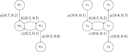
Example 2.
Consider the two PLTS over the Gödel algebra
 $M_1=\langle W_1,R_1,V_1\rangle$
and
 $M_2=\langle W_2,R_2,V_2 \rangle$
depicted bellow over the set
 $\{a,b,c,d\}$
of atomic actions. Function
 $h=\{w_1\mapsto v_1,w_2\mapsto v_2,w_3\mapsto v_3\}$
is a morphism from
 $M_1$
to
 $M_2$
.
In this setting, new pointed PLTS can be built compositionally. This section introduces the relevant operators, always parametric on the underlying iMTL-algebra
 $\boldsymbol{A}$
, by exploring the structure of the category of
 $\mathsf{Pt}_{\boldsymbol{A}}$
of pointed PLTS over
 $\boldsymbol{A}$
, that is whose objects are PLTS with a distinguished initial state and arrows in
 $\mathsf{Pt}_{\boldsymbol{A}}$
are allowed between PLTS with different sets of action symbols therefore generalizing the informal definition of morphism given above as follows:
Definition 3.
Let
 $T_1=\langle W_1,i_1,R_1 \rangle$
and
 $T_2 =\langle W_2,i_2,R_2 \rangle$
be two pointed PLTS over the set of atomic actions
 $\textrm{Act}_1$
and
 $\textrm{Act}_2$
, respectively. A morphism in
 $\mathsf{Pt}_{\boldsymbol{A}}$
from
 $T_1$
to
 $T_2$
consists on a pair of functions (
 $\sigma : W_1 \rightarrow W_2$
,
 $\lambda : \textrm{Act}_1 \rightarrow _{\bot }\textrm{Act}_2$
) such that
Footnote
1
 $\sigma (i_1)=i_2$
and for any
 $a \in \textrm{Act}_1$
,
 \begin{equation*}(R_1)_a(w,w') \, \preccurlyeq \, (R_2)^{\bot }_{\lambda (a)}(\sigma (w),\sigma (w'))\end{equation*}
For an accessibility relation
 $R$
,
 $R^{\bot }\,=\,R \cup R_\bot$
with
 $R_\bot (w,w)\,=\,(1,0)$
for any state
 $w \in W$
, denotes
 $R$
enriched with idle transitions in each state.
Clearly
 $\mathsf{Pt}_{\boldsymbol{A}}$
forms a category, whose composition in inherited from
 $\mathsf{Set}$
. Hence, as usual in categories of algebraic structures, most constructions in this Section build on the corresponding constructions in
 $\mathsf{Set}$
.
An algebra of PLTS typically includes some form of parallel composition, disjoint union, restriction, relabeling and prefixing, as one is used to from the process algebra literature (Baeten et al. Reference Baeten, Basten and Reniers2010). Accordingly, these operators are defined along the lines proposed by Winskel and Nielsen (Reference Winskel, Nielsen, Abramsky, Gabbay and Maibaum1995), for the standard, more usual case.
Restriction. The restriction operator is intended to control the interface of a transition system, preserving, in the case of a PLTS, the corresponding positive and negative weights. Formally,
Definition 4.
Let
 $T=\langle W,i,R,\textrm{Act} \rangle$
be pointed PLTS and
 $\lambda : \textrm{Act}' \rightarrow \textrm{Act}$
be an inclusion morphism. The restriction of
 $T$
to
 $\lambda$
,
 $T\upharpoonright \lambda$
, is a PLTS
 $\langle W,i,R'\rangle$
over
 $\textrm{Act}'$
such that, for any
 $w,v \in W$
and
 $a \in \textrm{Act}'$
,
 $R'_a(w,v)\,=\, R_a(w,v)$
There is a morphism
 $f=(1_W,\lambda )$
from
 $T\upharpoonright \lambda$
to
 $T$
, and a functor
 $P:\mathsf{Pt}_{\boldsymbol{A}} \to \mathsf{Set}_{\bot }$
which sends a morphism
 $(\sigma ,\lambda ):T\to T'$
to the partial function
 $\lambda :\textrm{Act}'\to \textrm{Act}$
. Clearly,
 $f$
is the Cartesian lifting of morphism
 $P(f)=\lambda$
in
 $\mathsf{Set}_{\bot }$
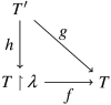
. Being Cartesian means that for any
 $g:T'\to T$
in
 $\mathsf{Pt}_{\boldsymbol{A}}$
such that
 $P(g)=\lambda$
there is a unique morphism
 $h$
such that
 $P(h)=1_{\textrm{Act} '}$
making the following diagram to commute:
Relabeling. In the same group of interface-modifier operators, is relabeling, which renames the labels of a PLTS according to a total function
 $\lambda :\textrm{Act} \rightarrow \textrm{Act}'$
.
Definition 5.
Let
 $T=\langle W,i, R , \textrm{Act}\rangle$
be a pointed PLTS and
 $\lambda : \textrm{Act} \rightarrow \textrm{Act}'$
be a total function. The relabeling of
 $T$
according to
 $\lambda$
is denoted by
 $T\{\lambda \}$
and it is the PLTS
 $\langle W,i,R'\rangle$
over
 $\textrm{Act}'$
where for any
 $w,v\in W$
and
 $a \in \textrm{Act}$
,
 $R'_{\lambda (a)}(w,v)\,=\,R_a(w,v)$
.
Dually to the previous case, there is a morphism
 $f=(1_W,\lambda )$
from
 $T$
to
 $T\{\lambda \}$
which is the cocartesian lifting of
 $\lambda$
(
 $= P(f)$
).
Parallel Composition. The product of two pointed PLTS combines their state spaces and includes all synchronous transitions, triggered by the simultaneous occurrence of an action of each component, as well as asynchronous ones in which a transition in one component is paired with an idle transition and valuations, labeled by
 $\bot$
, in the other. Formally,
Definition 6.
Let
 $T_1=\langle W_1,i_1,R_1, \textrm{Act}_1 \rangle$
and
 $T_2=\langle W_2,i_2,R_2, \textrm{Act}_2 \rangle$
be two pointed PLTS. Their parallel composition
 $T_1\times T_2$
is the PLTS
 $\langle W_1 \times W_2,(i_1,i_2),R, \textrm{Act}_1 \times _{\bot }\textrm{Act}_2 \rangle$
where,
 \begin{equation*}\textrm{Act}_1 \times _{\bot }\textrm{Act}_2\, =\, \{(a,\bot )\mid a\in \textrm{Act}_1\} \cup \{(\bot ,b)\mid b\in \textrm{Act}_2\}\cup \{(a,b)\mid a \in \textrm{Act}_1,b\in \textrm{Act}_2\}\end{equation*}
Such that,
 $R_{(a,b)}((w_1,w_2),(v_1,v_2)) \,=\, (\alpha , \beta )$
if and only if,
 $({R_1})^\bot _a(w_1,v_1) \, =\, (\alpha _1, \beta _1)$
and
 $({R_2})^\bot _b (w_2,v_2)\,=\,(\alpha _2,\beta _2)$
and
 $(\alpha ,\beta )\,=\, (\alpha _1,\beta _1) \mathrel {\substack {\land \\ \land }} (\alpha _2,\beta _2)$
.
Lemma 4.
Parallel composition is the product construction in
 $\mathsf{Pt}_{\boldsymbol{A}}$
.
Proof.
Let
 $T=\langle W,i,R, \textrm{Act} \rangle$
and
 $T_1=\langle W_1,i_1,R_1, \textrm{Act}_1\rangle$
be two pointed PLTS and let us define
 $T_1\times T_2=\langle W_1\times W_2,(i_1,i_2),R',\textrm{Act}'\rangle$
where
 $\textrm{Act}'= \textrm{Act}_1 \times _{\bot }\textrm{Act}_2$
according to Definition6. The projections
 $\pi _k: W_1 \times W_2 \to T_k$
defined as
 $\pi _k(w_1,w_2)\,=\, w_k$
for
 $k=1,\,2$
are morphisms in the
 $\mathsf{Pt}_{\boldsymbol{A}}$
category because
 $(R')_{(a,b)}((w_1,w_2),(v_1,v_2)) \,=\, (\alpha , \beta )$
if and only if,
 $({R_1})^\bot _a(\pi _1(w_1,w_2),\pi _1(v_1,v_2)) \, =\, (\alpha _1, \beta _1)$
and
 $({R_2})^\bot _b(\pi _2(w_1,w_2),\pi _2(v_1,v_2)) \, =\, (\alpha _2, \beta _2)$
and from
 $(\alpha ,\beta )\,=\, (\alpha _1,\beta _1) \mathrel {\substack {\land \\ \land }} (\alpha _2,\beta _2)$
follows
 $(\alpha ,\beta )\,\preccurlyeq \,(\alpha _1,\beta _1)$
and
 $(\alpha ,\beta )\,\preccurlyeq \,(\alpha _2,\beta _2)$
.
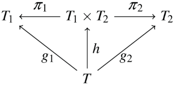
In the diagram below let
 $g_i=(\sigma _i,\lambda _i)$
, for
 $i = 1, 2$
, and define
 $h$
as
 $h = (\langle \sigma _1, \sigma _2 \rangle , \langle \lambda _1, \lambda _2 \rangle )$
, where
 $\langle f_1, f_2\rangle (x) = (f_1(x), f_2(x))$
is the universal arrow in a product diagram in
 $\mathsf{Set}$
. Clearly,
 $h$
lifts universality to
 $\mathsf{Pt}_{\boldsymbol{A}}$
, as the unique arrow making the diagram to commute. It remains show it is indeed an arrow in the category. By Definition6, for each
 $R_a(w,w')\,=\,(\alpha ,\beta )$
, there is a transition
 $(R_1)^\bot _{\lambda _1(a)}(\sigma _1(w),\sigma _1(w'))\,=\,(\alpha _1,\beta _1)$
such that
 $\alpha \leq \alpha _1$
and
 $\beta \geq \beta _1$
; and also a transition
 ${R_2}^{\bot }_{\lambda _2(a)}(\sigma _2(w) ,\sigma _2(w') ) \,=\,(\alpha _2,\beta _2)$
such that
 $\alpha \leq \alpha _1$
and
 $\beta \geq \beta _2$
. Moreover, there is a transition
 \begin{equation*}R'_{\langle \lambda _1,\lambda _2\rangle (a)}(\langle \sigma _1,\sigma _2\rangle (w),\langle \sigma _1,\sigma _2\rangle (w'))\,=\, (\alpha _1,\beta _1) \mathrel {\substack {\land \\ \land }} (\alpha _2,\beta _2)\end{equation*}
Thus, there is a transition
 $R'_{\langle \lambda _1,\lambda _2\rangle (a)}(\langle \sigma _1,\sigma _2\rangle (w), \langle \sigma _1,\sigma _2\rangle (w'))\,=\,(\alpha ',\beta ')$
, for any
 $R_a(w,w')\,=\,(\alpha ,\beta )$
, such that
 $\alpha \leq \alpha '$
and
 $\beta \geq \beta '$
. Furthermore,
 $\langle \sigma _1,\sigma _2\rangle (i) = (\sigma _1(i),\sigma _2(i))=(i_1,i_2)$
. This establishes
 $h$
as a
 $\mathsf{Pt}_{\boldsymbol{A}}$
morphism.
The following example illustrates the product of two pointed PLTS.
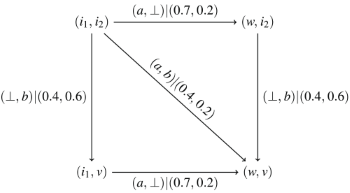
Example 3.
Consider the two PLTS,
 $T_1$
and
 $T_2$
depicted below.

Their product
 $T$
is the PLTS
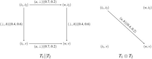
A suitable combination of parallel composition and restriction may enforce different synchronization disciplines. For example, interleaving or asynchronous product
 $T_1|| T_2$
is defined as
 $(T_1\times T_2) \upharpoonright \lambda$
with the inclusion
 $\lambda :\textrm{Act} \to \textrm{Act}_1\times _{\bot }\textrm{Act}_2$
for
 $\textrm{Act}=\{(a,\bot )\mid a\in \textrm{Act}_1\}\cup \{(\bot ,b)\mid b\in \textrm{Act}_2\}$
. This results in a PLTS
 $\langle W_1\times W_2,(i_1,i_2),R,\textrm{Act} \rangle$
such that for any
 $a \in \textrm{Act}$
, if
 $(R_2)_a(w,w')\,=\, (\alpha ,\beta )$
then
 $(R_1)_a(w,w')\,=\,(\alpha ,\beta )$
.
Similarly, the synchronous product
 $T_1\otimes T_2$
is also defined as
 $(T_1\times T_2) \upharpoonright \lambda$
, taking now
 $\textrm{Act}=\{(a,b)\mid a\in \textrm{Act}_1 \text{ and } b \in \textrm{Act}_2\}$
as the domain of
 $\lambda$
.
Example 4.
Interleaving and synchronous product of
 $T_1$
and
 $T_2$
as in Example
3
, are depicted below.
Sum. The sum of two pointed PLTS corresponds to their nondeterminisitic composition: the resulting PLTS behaves as either of its components. Formally,
Definition 7.
Let
 $T_1=\langle W_1,i_1,R_1, \textrm{Act}_1 \rangle$
and
 $T_2 = \langle W_2,i_2,R_2, \textrm{Act}_2 \rangle$
be two pointed PLTS. Their sum
 $T_1+T_2$
is the PLTS
 $\langle W,(i_1,i_2),R , \textrm{Act}\rangle$
with
 $\textrm{Act}=\textrm{Act}_1 \cup \textrm{Act}_2$
and
-
•
$W=(W_1\times \{i_2\}) \cup ( \{i_1\}\times W_2)$
-
•
$R_a((w_1,w_2),(v_1,v_2)) \,=\, (\alpha ,\beta )$
if and only if there is a transition
$(R_1)_a(w_1,v_1)\,=\,(\alpha ,\beta )$
or there is a transition
$(R_2)_a(w_2,v_2)\,=\,(\alpha ,\beta )$




Sum is actually a coproduct in
 $\mathsf{Pt}_{\boldsymbol{A}}$
(the proof follows the argument used for the product case), making
 $T_1+T_2$
dual to
 $T_1 \times T_2$
.
Example 5.
The sum
 $T_1 + T_2$
, for
 $T_1, T_2$
defined as in Example
3
is given by

Prefixing. As a limited form of sequential composition, prefix appends to a pointed PLTS a new initial state and a new transition to the previous initial state, after which the system behaves as the original one.
Definition 8.
Let
 $T=\langle W,i,R, \textrm{Act} \rangle$
be a pointed PLTS. Consider
 $w_{new}$
a fresh state identifier not in
 $W$
. Given an action
 $a \not \in \textrm{Act}$
, and
 $\alpha ,\beta \in A$
, the prefix
 $a|(\alpha ,\beta )T$
is defined as
 \begin{equation*}\langle W \cup \{w_{new}\},w_{new},R', \textrm{Act}\cup \{a\} \rangle \end{equation*}
where
 $R'_b(w,v)\,=\, R_b(w,v)$
if
 $b \in \textrm{Act}$
and
 $R'_a(w_{new}, i)\,=\,( \alpha ,\beta )$
.
Since it is not required that the prefixing label is distinct from the ones in the original system, prefixing does not extend to a functor in
 $\mathsf{Pt}_{\boldsymbol{A}}$
, as illustrated in the counterexample below. This is obviously the case for a category of classical labeled transition systems as well. In both cases, however, prefix extends to a functor if the corresponding categories are restricted to action-preserving morphisms, that is, in which the action component of a morphism is always an inclusion
Example 6.
Consider two pointed PLTS
 $T_1$
and
 $T_2$

connected by a morphism
 $(\sigma ,\lambda ):T_1\to T_2$
such that
 $\sigma (i_1)=i_2$
,
 $\sigma (w)=v$
and
 $\lambda (a)=b$
. Now consider the prefixes
 $a|(1,0)T_1$
and
 $a|(1,0)T_2$
depicted below.


Clearly, a mapping from the actions in
 $a|(1,0)T_1$
to the actions in
 $a|(1,0)T_1$
does not exist so neither exists a morphism between the two systems.
Functorial Extensions. Other useful operations between pointed PLTS, typically acting on transitions’ positive and negative weights, and whose definition depends on the specific residuated lattice chosen, can be defined functorially in
 $\mathsf{Pt}_{\boldsymbol{A}}$
. An example involving a pointed PLTS defined over a Gödel algebra is an operation that uniformly increases or decreases the value of the positive (or the negative, or both) weight in all transitions. Let
 \begin{equation*}\alpha \oplus \beta =\begin{cases} 1 \text{ if } \alpha +\beta \geq 1\\0\text{ if } \alpha +\beta \leq 0\\ \alpha +\beta \text{ otherwise } \end{cases}\end{equation*}
Thus,
Definition 9.
Let
 $T=\langle W,i,R, \textrm{Act} \rangle$
be a pointed PLTS. Taking
 $v\in [-1,1]$
, the positive
 $v$
-approximation
 ${T_{\oplus }}^+_v$
is a pointed PLTS
 $\langle W,i,R', \textrm{Act} \rangle$
where for any relation
 $R_a(w,w')\,=\,(\alpha ,\beta )$
we define
 $R'_a(w,w')\,=\, (\alpha \oplus v, \beta )$
.
The definition extends to a functor in
 $\mathsf{Pt}_{\boldsymbol{A}}$
which is the identity in morphisms. Similar operations can be defined to act on the negative accessibility relation or both.
Another useful operation removes all transitions in a pointed PLTS for which the positive accessibility relation is below a certain value and the negative accessibility relation is above a certain value. Formally,
Definition 10.
Let
 $T=\langle W,i,R, \textrm{Act} \rangle$
be a pointed PLTS. For
 $p, n\in [0,1]$
, the purged PLTS
 $T_{{p}\uparrow \downarrow {n}}$
is defined as
 $\langle W,i,R', \textrm{Act} \rangle$
where
 \begin{equation*}R'_a(w,w')\,=\, \begin{cases} R_a(w,w') & \text{if } (p,m) \, \preccurlyeq \, R_a(w,w') \\ (0,1) & \text{otherwise} \end{cases}\end{equation*}
Clearly, the operation extends to a functor in
 $\mathsf{Pt}_{\boldsymbol{A}}$
, mapping morphisms to themselves.
4. From PLTS to Paraconsistent Kripke Models: Crisp and Graded Bisimulations
Having introducing PLTS and their algebra, this section goes another step ahead. Stating and proving properties of such systems entails the need for a suitable modal logic to explore their (double) transition structure. We start in this section by endowing PLTS with propositions that take values on
 $A \times A$
, therefore providing a corresponding notion of a paraconsistent Kripke model. Two approaches to defining simulation and bisimulation over them, one crisp, as in the original paper (Cruz et al. Reference Cruz, Madeira, Barbosa, Indrzejczak and Zawidzki2022b), and another graded are discussed. We start with the following definition:
Definition 11.
A paraconsistent Kripke model over a iMTL-algebra
 $\boldsymbol{A}$
, a set of atomic actions
 $\textrm{Act}$
and a set of proposition symbols
 $\textrm{Prop}$
is a structure
 $\langle W,R,V\rangle$
where
 $\langle W, R \rangle$
is a paraconsistent transition system and
 $V:W\times \textrm{Prop} \rightarrow A \times A$
is a valuation function that for a proposition
 $p \in \textrm{Prop}$
and state
 $w \in W$
,
 $V(w,p)\,=\,(\alpha , \beta ) \in A \times A$
means that
 $\alpha$
weights the evidence of
 $p$
holding at state
 $w$
and
 $\beta$
weights the evidence of
 $p$
not holding at
 $w$
.
Paraconsistent Kripke models can be related by simulation or bisimulation relations, either crisp or graded, as discussed in the sequel. As before, all constructions are parametric in the underlying iMTL-algebra
 $\boldsymbol{A}$
, whose explicit reference is, from now on, omitted.
Crisp Simulation and Bisimulation
Definition 12.
Let
 $M=\langle W,R,V\rangle$
and
 $M'=\langle W',R',V' \rangle$
be two paraconsistent models over a set of action symbols
 $\textrm{Act}$
and another of propositions
 $\textrm{Prop}$
. A relation
 $S \subseteq W \times W'$
is a simulation provided that, for all
 $(w,w') \in S$
,
 $p \in \textrm{Prop}$
and
 $a \in \textrm{Act}$
-
•
$V(w,p) \, \preccurlyeq \, V'(w',p)$
, and
-
•
$R_a(w,v)\,=\, (\alpha ,\beta )$
then exists
$v'\in W', \, \gamma ,\delta \in A$
such that
$R'_a(w',v')\,=\, (\gamma ,\delta )$
and
$ R_a(w,v) \,\preccurlyeq \, R'_a(w',v')$
and
$(v,v') \in S$






Whenever one restricts in the definition above to the existence of values
 $\gamma$
(resp.
 $\delta$
) such that
 $\gamma \geq \alpha$
(resp.
 $\delta \leq \beta$
), the corresponding simulation is called positive (resp. negative).
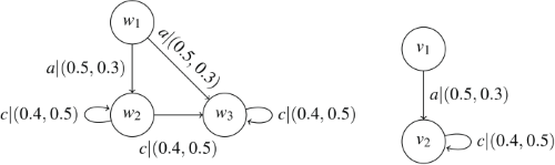
Example 7. Recall the PLTS depicted above over the empty set of proposition symbols. The following relation is a crisp simulation,
 \begin{equation*}S=\{ (w_1,v_1),(w_2,v_2), (w_3,v_2), (w_4,v_3), (w_5,v_4)\}\end{equation*}
Definition 13.
Let
 $M\,=\, \langle W,R,V\rangle$
and
 $M'\,=\, \langle W',R',V' \rangle$
be two paraconsistent models over the set of actions
 $\textrm{Act}$
and the set of propositions
 $\textrm{Prop}$
. A relation
 $B \subseteq W \times W'$
is a bisimulation if for
 $(w,w') \in B$
,
 $p \in \textrm{Prop}$
and
 $a \in \textrm{Act}$
the following conditions hold:
-
•
$V(w,p) \, = \, V'(w',p)$
, and
-
• for any
$v \in W$
such that
$R_a(w,v)\,=\, (\alpha ,\beta )$
, there is
$v'\in W'$
such that
$R'_a(w',v')\,=\, (\alpha ,\beta )$
and
$(v,v') \in S$
-
• for any
$v' \in W'$
such that
$R'_a(w',v')\,=\, (\alpha ,\beta )$
, there is
$v\in W$
such that
$R_a(w,v)\,=\, (\alpha ,\beta )$
and
$(v,v') \in S$











Example 8. Consider the two paraconsistent models depicted below.
with
 $V_1(w,p)\,=\,V_2(v_1,p)$
and
 $V_1(w_2,p)\,=\,V_1(w_3,p)\,=\,V_2(v_2,p)$
for any proposition symbol
 $p$
. The relation
 $B\,=\, \{ (w_1,v_1), (w_2,v_2),(w_3,v_3)\}$
is a crisp bisimulation.
Graded Simulation and Bisimulation
When comparing paraconsistent transition structures, a more intuitive approach consists of treating bisimulation as a graded relation, encompassing both positive and negative weights. This relation, we refer to as paraconsistent bisimulation, follows the lines of work documented in Nguyen (Reference Nguyen2022) for fuzzy modal logic. This subsection generalizes (Nguyen Reference Nguyen2022) approach for paraconsistent modal logic and discusses its, slightly weird, expressivity.
Definition 14.
Let
 $M\,=\, \langle W,R,V\rangle$
and
 $M'\,=\, \langle W',R',V' \rangle$
be two paraconsistent models over a iMTL-algebra
 $\boldsymbol{A}$
and a set
 $Act$
of actions. A relation
 $S^G: W \times W' \rightarrow A \times A$
is a
graded simulation
if the following conditions hold for all
 $p \in \textrm{Prop}, \, a \in \textrm{Act}$
and all possible values of free variables:
 \begin{align}&\qquad\qquad\qquad S^G(w,w') \preccurlyeq (V(w,p) \Rightarrow V'(w',p)) \end{align}
 \begin{align}& \exists v' \in W', \; (S^G(w,w') \otimes R_a(w,v)) \preccurlyeq (R'_a(w',v') \otimes S^G(v,v')) \end{align}
It is worth noticing that the crisp simulation is not a particular case of the graded simulation. The following two examples discuss this issue.
Example 9.
Consider the following paraconsistent model with one proposition
 $p$
:

with
 $V(w,p)\,=\,V'(w',p)\,=\,(1,0)$
. Since
 $V(w,p) \, \preccurlyeq \, V'(w',p)$
and
 $R_a(w,w) \, \preccurlyeq \, R'_a(w',w')$
relation
 $S=\{(w,w')\}$
is a crisp simulation, i.e., it is possible to informally write
 $S(w,w')\,=\,(1,0)$
since there is complete evidence that states
 $w$
and
 $w'$
are similar and absolute minimal evidence that they are not. Notice that
 $S(w,w')\,=\,(1,0)$
satisfies conditions
(31)
and
(32)
, that is,
 \begin{equation*}(1,0) \, \preccurlyeq \, V(w,p) \Rightarrow V'(w',p) \, =\,(1,0)\end{equation*}
 \begin{equation*}(1,0) \otimes (1,1) \,\preccurlyeq \,(1,0) \otimes (1,0) \end{equation*}
Thus,
 $S(w,w')\,=\,(1,0)$
is also a graded simulation. Since any graded simulation is bounded by the pair
 $(1,0)$
we have that
 $S(w,w')\,=\,(1,0)$
is the biggest graded simulation between the two paraconsistent models. Actually, while the notion of a crisp simulation is bivalent, that is, either states are or are not similar, in a graded simulation that is not the case. It is often possible to define other graded simulations that satisfy all conditions. For example, the relation
 $S'(w,w')\,=\,(0.5,0.5)$
is also a graded simulation between the models that satisfies
(31)
and
(32)
.
Example 10.
Consider now the following paraconsistent model assuming
 $(1,0)$
as the value of proposition
 $p$
in all states.
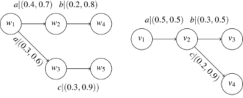
The following relation is a graded simulation
 \begin{align*} &S^G(w_1,v_1)\,=\,S^G(w_2,v_2)\,=\, S^G(w_4,v_3)\,=\, S^G(w_5,v_4)\,=\,(1,0) \\ &S^G(w_3,v_2)=(0.2,1) \end{align*}
Transitions from state
 $w_3$
to
 $w_5$
and from state
 $v_2$
to
 $v_4$
are similar with equal negative weights, i.e.
 $R^-_c(w_3,w_5) \, = \, {R'}^-_c(v_2,v_4)$
. However, despite the transitions being similar, as per the definition of a crisp simulation, there is no crisp simulation
 $S$
such that
 $(w_3,v_2) \in S$
. However, when considering a graded simulation, a different perspective emerges. There is complete evidence that the states are not similar, as witnessed by the crisp relation, while simultaneously indicating some evidence,
 $0.2$
, of their similarity.
Let us take this question a little further and investigate under which conditions graded simulation coincides with the crisp simulation. Consider paraconsistent models
 $M=\langle W,R,V\rangle$
,
 $M'=\langle W',R',V' \rangle$
and a crisp simulation
 $S$
between them. Consider any pair of states
 $(w,w') \in W \times W'$
such that
 $(w,w') \in S$
. Is there a graded simulation
 $S^G: W \times W' \rightarrow A \times A$
such that
 $S^G(w,w')\,=\,(1,0)$
? In other words, if two states are related by a crisp simulation, is there a graded simulation relating them with weight
 $(1,0)$
, that is, is there complete evidence that the states are similar and absolute minimal evidence that they are not similar?
For some proposition symbol
 $p$
and action symbol
 $a$
, consider
 $V(w,p)\,=\,(\gamma ,\delta )$
,
 $V'(w',p)\,=\,(\gamma ',\delta ')$
,
 $R_a(w,v)\,=\, (\alpha , \beta )$
and
 $R'_a(w',v')=(\alpha ',\beta ')$
. Since
 $(w,w') \in S$
, it follows that
 $(\gamma ,\delta ) \, \preccurlyeq \, (\gamma ',\delta ')$
and
 $ (\alpha , \beta ) \, \preccurlyeq \, (\alpha ', \beta ')$
, as well as,
 $(v,v') \in S$
. Let us now evaluate if it is possible to have a graded simulation such that
 $S^G(w,w') \,=\,(1,0)$
, or without loss of generality,
 $S^G(w,w') \,\preccurlyeq \,(1,0)$
. Relation
 $S^G$
must satisfy condition (31),
 \begin{align*} S^G(w,w') & \preccurlyeq V(w,p) \Rightarrow V'(w',p) \\ & \scriptstyle {\{\text{defn of }\Rightarrow \}} \\ & = \; ( (\gamma \to \gamma ') \land (\delta ' \to \delta ), \gamma \land \delta ') \\ & \scriptstyle {\{\text{Hypothesis: }\gamma \leq \gamma '\text{ and }\delta \geq \delta '\}} \\ & =\; (1, \gamma \land \delta ') \end{align*}
Thus, from condition (31),
 $S^G(w,w') \, \preccurlyeq \, (1,0)$
implies
 $\gamma =0$
or
 $\delta '=0$
. Relation
 $S^G$
must also satisfy condition (32),
 \begin{equation*}S^G(w,w') \otimes R_a(w,v) \, \preccurlyeq \, R'_a(w',v') \otimes S^G(v,v')\end{equation*}
Using adjunction (17),
 $S^G(w,w') \, \preccurlyeq \, R_a(w,v) \Rightarrow (R'_a(w',v') \otimes S^G(v,v'))$
. Thus,
 \begin{align*} S^G(w,w') \; & \preccurlyeq \; R_a(w,v) \Rightarrow (R'_a(w',v') \otimes S^G(v,v')) \\ & \scriptstyle {\{\text{$S^G(v,v') \, \preccurlyeq \, (1,0)$ by (19) and (18)}\}} \\ & \preccurlyeq \; R_a(w,v) \Rightarrow (R'_a(w',v') \otimes (1,0)) \\ & \scriptstyle {\{\text{defn of }\otimes \}} \\ &= \; R_a(w,v) \Rightarrow (\alpha ', (\alpha ' \to 0) \land \beta ')\\ & \scriptstyle {\{\text{defn of }\Rightarrow \}} \\ & = \; ((\alpha \to \alpha ') \land (((\alpha ' \to 0) \land \beta ') \to \beta ), \alpha \land \alpha ' \to 0 \land \beta ')\\ & \scriptstyle {\{\text{Hypothesis: }\alpha \leq \alpha '\text{ and }\beta ' \leq \beta \}} \\ & = \; (1, \alpha \land (\alpha ' \to 0) \land \beta ') \end{align*}
Thus, from condition (32),
 $S^G(w,w') \, \preccurlyeq \, (1,0)$
implies
 $\alpha =0$
or
 $\beta '=0$
or
 $\alpha ' \gt 0$
.
In conclusion, if
 $(w,w') \in S$
there is a graded simulation
 $S^G$
such that
 $S^G(w,w')\,=\,(1,0)$
only when
 $V^+(w,p)=0$
or
 ${V'}^-(w',p)=0$
and either
 $R^+_a(w,v)=0$
or
 ${R'}^-_a(w',v')=0$
or
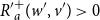 ${R'}^+_a(w',v') \gt 0$
.
This discussion sheds light on a somehow surprising conclusion: that identity fails to be a simulation. Actually, consider the following paraconsistent models,

with
 $V(w,p)\,=\,V'(w',p)\,=(0.2,0.2)$
. The relation
 $S^G(w,w') =(1,0)$
is not a graded simulation because

Definition 15.
Let
 $M\,=\, \langle W,R,V\rangle$
and
 $M'=\langle W',R',V' \rangle$
be paraconsistent models over a iMTL-algebra
 $\boldsymbol{A}$
and a set
 $Act$
of actions. A relation
 $B^G: W \times W' \rightarrow A \times A$
is a
graded bisimulation
if the following conditions hold for all
 $p \in \textrm{Prop}, \, a \in \textrm{Act}$
and all possible values of free variables:
 \begin{align}&\qquad\qquad\quad B^G(w,w') \preccurlyeq (V(w,p) \Leftrightarrow V'(w',p)) \end{align}
 \begin{align}& \exists v' \in W', \; (B^G(w,w') \otimes R_a(w,v)) \preccurlyeq (R'_a(w',v') \otimes B^G(v,v')) \end{align}
 \begin{align}&\, \exists v \in W, \; (B^G(w,w') \otimes R'_a(w',v')) \preccurlyeq (R_a(w,v) \otimes B^G(v,v')) \end{align}
Again a crisp bisimulation is not, in general, a particular case of a graded one, as illustrated in the following examples.
Example 11.
Consider the paraconsistent models depicted below where
 $V(w_1,p)\,=\, V'(v_1,p)\,=\,(0,1)$
,
 $V(w_2,p)\,=\,V'(v_2,p)\,=\,(1,0)$
and
 $V(w_3,p)\,=\,V'(v_3,p)\,=\,(0,0)$
.
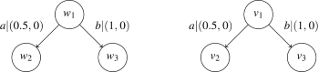
Clearly,
 $B=\{(w_1,v_1),(w_2,v_2),(w_3,v3)\}$
is a crisp bisimulation. Informally,
 $B$
can be written as a graded bisimulation
 $B^G: W\times W \rightarrow A \times A$
where
 $B^G(w_1,v_1)\,=\,B^G(w_2,v_2)\,=\,B^G(w_3,v_3)\,=\,(1,0)$
. Notice that,
 $B^G$
satisfies condition
(33)
,
 \begin{align*} & (1,0) \, \preccurlyeq \, (0,1) \Leftrightarrow (0,1) \,=\, (1,0)\\ & (1,0) \, \preccurlyeq \, (1,0) \Leftrightarrow (1,0) \,=\, (1,0)\\ & (1,0) \, \preccurlyeq \, (0.5,0) \Leftrightarrow (0.5,0) \,=\, (1,0) \end{align*}
and conditions (34) and (35) ,
 \begin{align*} & (1,0) \otimes (0.5,0) \,=\, (0.5,0) \, \preccurlyeq \, (0.5,0)\otimes (1,0) \,=\, (0.5,0)\\ & (1,0) \otimes (1,0) \,=\, (1,0) \, \preccurlyeq \, (1,0)\otimes (1,0) \,=\, (1,0) \end{align*}
Example 12. For an example in the opposite direction, consider
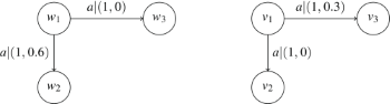
where
 $V(w_1,p)\,=\,V'(v_1,p)\,=\,(1,1), \, V(w_2,p)\,=\,V'(v_3,p)\,=\, (1,0.5)$
and
 $V(w_3,p)\,=\, V'(v_2,p)\,=\,(0.8,0.8)$
. A graded bisimulation
 $B^G$
between the above paraconsistent models can be computed as follows:
-
• From condition (33) ,
\begin{align*} B^G(w_1,v_1)\, & \preccurlyeq \, (1,1) \Leftrightarrow (1,1)\,=\, (1,1)\\ B^G(w_2,v_2) \, & \preccurlyeq \, (1,0.5) \Leftrightarrow (0.8,0.8)\, =\, (0.5,0.8) \\ B^G(w_3,v_3)\, & \preccurlyeq \, (0.5,0.8)\\ B^G(w_2,v_3)\, & \preccurlyeq \, (1,0.5)\\ B^G(w_3,v_2)\, & \preccurlyeq \, (1,0.8) \end{align*}
-
• From condition (34) , on the other hand,
Thus,
\begin{equation*}B^G(w_1,v_1) \otimes R_a(w_1,w_2) \, \preccurlyeq \, R'_a(v_1,v_2) \, \otimes B^G(w_2,v_2)\, \preccurlyeq \, (1,0) \otimes (0.5,0.8) = (0.5,0)\end{equation*}
${B^G}^+(w_1,v_1) \land 1\,=\, {B^G}^+(w_1,v_1)\, \leq 0.5$
. Similarly,
Thus,
\begin{equation*}B^G(w_1,v_2) \otimes R_a(w_1,w_2) \, \preccurlyeq \, R'_a(v_2,v_2) \, \otimes B^G(w_2,v_2)\, \preccurlyeq \, (0,1) \otimes (0.5,0.8) = (0,1)\end{equation*}
$B^G(w_1,v_2)\,=\,(0,1)$
. A similar reasoning yields
$B^G(w_1,v_3)\,=\,(0,1)$
.
-
• Finally, from condition (35) , we conclude that
$B^G(w_2,v_1)\,=\,B^G(w_3,v_1)\,=\,(0,1)$
.







Therefore, one possible graded bisimulation between the paraconsistent models is
 $B^G(w_1,v_1)\,=\,(0.5,1)$
,
 $B^G(w_2,v_2)\,=\,(0.5,0.8)$
,
 $B^G(w_2,v_3)\,=\,(1,0.5)$
,
 $B^G(w_3,v_2)\,=\, (1,0.8)$
and
 $B^G(w_3,v_3)\,=\,(0.5,0.8)$
since it satisfies conditions
(33)
-
(35)
. The figure below depicts this graded bisimulation through red dashed lines.
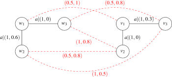
Once again, we may ask which conditions are necessary for crisp and graded bisimulations to match. Consider paraconsistent models
 $M=\langle W,R,V\rangle$
,
 $M'=\langle W',R',V' \rangle$
and a crisp bisimulation
 $B$
between them. Consider any pair of states
 $w \in W,\, w' \in W'$
such that
 $(w,w') \in B$
. Is there a graded bisimulation
 $B^G: W \times W' \rightarrow A \times A$
such that
 $B^G(w,w')\,=\,(1,0)?$
If
 $(w,w') \in B$
there is a graded bisimulation
 $B^G$
such that
 $B^G(w,w')\,=\,(1,0)$
only if
 $V^+(w,p)\,=\,0$
or
 $V^-(w,p)=0$
and either
 $R^+_a(w,v)=0$
or
 ${R'}^-_a(w',v')=0$
or
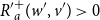 ${R'}^+_a(w',v') \gt 0$
and either
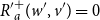 ${R'}^+_a(w',v')=0$
or
 $R^-_a(w,v)=0$
or
 $R^+_a(w,v) \gt 0$
.
5. A Modal Logic for Paraconsistent Models
The Logic
We are now able to introduce a modal logic
 $\textrm{P}(\boldsymbol{A})$
to specify properties of paraconsistent structures parametric on an iMTL-algebra
 $\boldsymbol{A}$
.
Definition 16.
Given an iMTL-algebra
 $\boldsymbol{A}$
, a set of proposition symbols
 $\textrm{Prop}$
and a set of action symbols
 $\textrm{Act}$
, the set of sentences
 $\mathsf{Sen}(\textrm{Prop},\textrm{Act})$
of
 $\textrm{P}(\boldsymbol{A})$
is generated by the following grammar:
 \begin{equation*} \varphi \, := \, \bot \,| \, p\, |\, \neg \varphi \, |\, \varphi \land \varphi \, | \, \langle a \rangle \varphi \end{equation*}
where
 $p \in \textrm{Prop}$
and
 $a \in \textrm{Act}$
. As usual, the following abbreviations are considered:
 $\top \, =\, \neg \bot$
,
 $\varphi \lor \varphi ' \, = \, \neg (\neg \varphi \land \neg \varphi ')$
,
 $\varphi \triangleright \varphi '\,=\, \neg \varphi \lor \varphi ' \,=\, \neg (\varphi \land \neg \varphi ')$
,
 $\varphi \diamond \varphi '\,=\, (\varphi \triangleright \varphi ') \land (\varphi ' \triangleright \varphi )$
and
 $[a]\varphi \,=\, \neg \langle a \rangle \neg \varphi$
.
For a given paraconsistent model
 $M$
, which the underlying iMTL-algebra is
 $\boldsymbol{A}$
, the satisfaction relation in
 $\textrm{P}(\boldsymbol{A})$
associates to
 $M$
and a sentence
 $\varphi$
a pair of weights
 $(\alpha ,\beta ) \in A \times A$
. As before, the positive weight
 $\alpha$
stands for the evidence that
 $\varphi$
holds in
 $M$
while the negative weight
 $\beta$
stands for the evidence of the opposite fact.
Definition 17.
Let
 $\boldsymbol{A}\,=\,\langle A, \land , \lor ,1,0,\to \rangle$
be an iMTL-algebra and
 $M\,= \, \langle W,R,V\rangle$
a paraconsistent model. The satisfaction relation,
 \begin{equation*}\models \, : \, M \times \mathsf{Sen}(\textrm{Prop}, \textrm{Act}) \,\rightarrow \, A \times A\end{equation*}
is given by
 \begin{equation*}(M \models \varphi ) \,=\, \underset {w \in W}{\mathrel {\substack {\land \\ \land }}}\,(M,w \models \varphi )\end{equation*}
where relation
 $\models$
is recursively defined as follows,
-
•
$(M,w \models \bot ) \, =\, (0,1)$
-
•
$(M,w \models p) \,=\, V(w,p)$
-
•
$(M, w \models \neg \varphi )\,=\, \mathbin {/\mkern -6mu/} (M,w \models \varphi )$
-
•
$(M, w \models \varphi \land \varphi ') \, =\, (M,w \models \varphi ) \mathrel {\substack {\land \\ \land }} (M,w\models \varphi ')$
-
•
$(M,w \models \langle a \rangle \varphi ) \,=\, \underset {v \in W}{\mathrel {\substack {\lor \\ \lor }}} \, \bigg ( R_a(w,v) \otimes (M,v \models \varphi ) \bigg )$





Informally, sentence
 $\varphi$
is evaluated at each state of the model
 $M$
and
 $(a,b)$
is the result of the conjunction of each of these evaluations. Hence, a sentence
 $\varphi$
is said to be valid if, for any state
 $w \in W$
,
 $(M,w \models \varphi )\,=\, (1,0)$
, that is there is complete evidence that
 $\varphi$
holds at state
 $w$
and absolute minimal evidence that it does not hold. Note how the operators characterizing the twist-structure introduced earlier in the paper reappear in the satisfaction relation to take care of pairs of weights being computed.
The next example emphasizes the fact that paraconsistent models generalize transition structures in which the information is consistent, that is, in which the transition relation and the valuation function are either
 $(1,0)$
or
 $(0,1)$
.
Example 13.
Consider the set
 $\textrm{Act}=\{a,b,c\}$
of action symbols and the set
 $\textrm{Prop}=\{p\}$
of propositions. Let
 $M$
be the following paraconsistent model over the Gödel algebra with
 $V(w_1,p)\; =\; V(w_3,p)\,=\,(1,0)$
and
 $V(w_2,p)\,=\,(0,1)$
.

Then,
 \begin{align*} (M,w_2 \models \langle c \rangle p \land [a] \neg p) =\; & \bigg (M,w_2 \models \langle c \rangle p \bigg ) \, \mathrel {\substack {\land \\ \land }}\, \bigg (M,w_2 \models [a] \neg p \bigg ) \\ =\; & \bigg ((R_c(w_2,w_1) \otimes (M,w_1 \models p)\bigg ) \, \mathrel {\substack {\land \\ \land }} \, \bigg (M,w_2 \models \neg \langle a \rangle \neg \neg p\bigg )\\ =\; & \bigg ( (1,0) \otimes (1,0) \bigg ) \, \mathrel {\substack {\land \\ \land }} \, \mathbin {/\mkern -6mu/} \bigg ( M,w_2 \models \langle a \rangle p\bigg ) \\ =\; & (1 \land 1, 1 \to 0 \land 1 \to 0) \, \mathrel {\substack {\land \\ \land }} \, \mathbin {/\mkern -6mu/} \bigg ( R_a(w_2,w_3) \otimes (M, w_3 \models p)\bigg )\\ =\; & (1,0) \, \mathrel {\substack {\land \\ \land }} \, \mathbin {/\mkern -6mu/} \bigg ( (1,0) \otimes (0,1) \bigg ) \, =\; (1,0) \, \mathrel {\substack {\land \\ \land }} \, \mathbin {/\mkern -6mu/}(0,1)\\ =\; & \,(1 \land 1, 0 \lor 0) \\ =\; & (1,0) \end{align*}
Informally, this can be read as follows: at state
 $w_2$
there is a transition through action
 $c$
to a state where
 $p$
holds and all transitions through action
 $a$
reach a state where
 $p$
does not hold. As expected, the result is a consistent pair of weights
 $(1,0)$
, that is, there is complete evidence,
 $1$
, that this sentence holds at state
 $w_2$
and absolute non evidence,
 $0$
, evidence that it does not hold.
Example 14.
Consider another paraconsistent model over the Gödel algebra, with
 $\textrm{Act}=\{a,b\}$
and
 $Prop=\{p,q,r\}$

with,
 $V(w,p)\,=\,(1,1)$
,
 $V(w,q)\,=\,V(v,p)\,=\,(0,0.5)$
,
 $V(w,r)\,=\,V(v,r)\,=\, (0.5,0.5)$
and
 $V(v,q)\,=\,(0,0)$
. Then,
 \begin{align*} (M,w \models r \triangleright (p \lor q) ) = \; & (M, w \models \neg r \lor (p \lor q)) \\ =\; & (M, w\models \neg ( \neg \neg r \land \neg (p \lor q))) \\ =\; & \mathbin {/\mkern -6mu/} \bigg ( M,w \models r \land \neg (p \lor q) \bigg ) \\ =\; & \mathbin {/\mkern -6mu/} \bigg ( (M,w \models r) \,\mathrel {\substack {\land \\ \land }}\,( M,w \models \neg (p \lor q)) \bigg ) \\ =\; & \mathbin {/\mkern -6mu/} \bigg ( V(w,r) \, \mathrel {\substack {\land \\ \land }}\, \mathbin {/\mkern -6mu/} (M, w \models p \lor q) \bigg )\\ =\: & \mathbin {/\mkern -6mu/} \bigg ( V(w,r) \, \mathrel {\substack {\land \\ \land }} \, (M,w \models \neg p) \mathrel {\substack {\land \\ \land }} (M,w \models \neg q) \bigg ) \\ =\: & \mathbin {/\mkern -6mu/} \bigg ( V(w,r) \, \mathrel {\substack {\land \\ \land }} \, \mathbin {/\mkern -6mu/} V(w,p) \, \mathrel {\substack {\land \\ \land }} \, \mathbin {/\mkern -6mu/} V(w,q) \bigg ) \\ =\; & \mathbin {/\mkern -6mu/} \bigg ( (0.5,0.5) \, \mathrel {\substack {\land \\ \land }} \, (1,1) \, \mathrel {\substack {\land \\ \land }} \, (0.5,0) \bigg )\\ =\; & \mathbin {/\mkern -6mu/} (0.5 \land 1 \land 0.5, 0.5 \lor 1 \lor 0)\,=\, \mathbin {/\mkern -6mu/}(0.5,1) \\ =\; & (1,0.5) \end{align*}
Similarly,
 $(M,v \models r \triangleright (p \lor q) ) \,=\, (0.5,0)$
. Therefore,
 \begin{equation*}M \models r \triangleright (p \lor q) \, =\, (1,0.5) \mathrel {\substack {\land \\ \land }} (0.5,0) \,=\, (0.5,0.5)\end{equation*}
giving
 $0.5$
evidence that the sentence
 $r \triangleright (p \lor q)$
holds and does not hold in this paraconsistent model.
Properties
This subsection presents some preliminary results on soundness of paraconsistent Kripke models. The crucial ingredient is that we generalize the classical notion of soundness, where both premises and conclusions are consistently true, and instead, introduce a graded notion of soundness, where both premises and conclusions may encompass vagueness and contradictions.
As stated in the introduction, a similar motivation can be found in Caicedo and Rodríguez (Reference Caicedo and Rodríguez2010) where the authors introduce a notion of logical consequence, denoted by
 $\models _{\leq \text{GK}}$
, for Gödel Kripke models
 $\text{GK}$
. They then proceed to prove the soundness of the
 $\square$
-fragment (and similarly of the
 $\diamond$
-fragment). However, it is important to note that the main results highlighted in Caicedo and Rodríguez (Reference Caicedo and Rodríguez2010) pertain to countable theories, where the notions of classical logical consequence
 $\models _{GK}$
and
 $\models _{\leq \text{GK}}$
are equivalent. Our approach for paraconsistent Kripke models is similar, as we also consider classical and graded notions of soundness, the latter of which we term as g-soundness. This graded variant adjusts the classical definition of soundness to accommodate vague and inconsistent evaluations. It is evident that g-soundness is a more relaxed notion than classical soundness, thus implying that g-soundness entails classical soundness. However, the converse is not true, leading us to explore soundness results in Kripke paraconsistent models where g-soundness and classical soundness are not equivalent. In summary, the main results documented are:
-
• Modus Ponens (MP) and Modal Generalization (Gen) rules are classically sound but not g-sound;
-
• Distribution of the possibility operator over
$\lor$
and
$\land$
, rules (36) and (37), are sound and g-sound. -
• Distribution of the necessity operator over
$\triangleright$
, rule (K), is neither sound nor g-sound.


Let us start by revisiting the classical notion of soundness and then introduce its graded counterpart, extending upon the classical understanding. Following that, we will conduct a preliminary investigation into the properties of soundness for paraconsistent Kripke models.
Definition 18. A rule
 \begin{equation*} \frac {\varphi _1\;\ldots \; \varphi _n}{\varphi } \end{equation*}
is sound if for any paraconsistent Kripke structure
 $M=\langle W,R,V\rangle$
,
 \begin{equation*} \text{if } (M \models \varphi _i)\,=\,(1,0) \text{ for } i \in \{1, \ldots , n\} \text{, then } (M \models \varphi )\,=\,(1,0)\end{equation*}
The following, alternative, notion of soundness accommodates vague and inconsistent evaluations, implying that from the evidence of truth and falsity of premises, it is possible to draw conclusions whose evidence of truth is higher and of falsity lower.
Definition 19. A rule
 \begin{equation*} \frac {\varphi _1\;\ldots \; \varphi _n}{\varphi } \end{equation*}
is g-sound if for any paraconsistent Kripke structure
 $M=\langle W,R,V\rangle$
,
 \begin{equation*}\underset {i=1}{\overset {n}{\mathrel {\substack {\land \\ \land }}}} (M \models \varphi _i) \preccurlyeq \, (M \models \varphi )\end{equation*}
The following theorem is crucial for subsequent steps because it assures that g-soundness generalizes classical soundness.
Theorem 1. If a rule is g-sound, then it is sound.
Proof.
Consider a g-sound rule whose premises are
 $\varphi _1\;\ldots \; \varphi _n$
and conclusion
 $\varphi$
. We must prove that this rule is sound. Let us fix a paraconsistent Kripke structure
 $M=\langle W,R,V\rangle$
such that the premises are consistently true, that is,
 $(M\models \varphi _i)\,=\,(1,0)$
for any
 $i \in \{1,\ldots , n\}$
. By hypothesis
 \begin{equation*} (M \models \varphi _1)\, \mathrel {\substack {\land \\ \land }} \, (M \models \varphi _2) \,\mathrel {\substack {\land \\ \land }} \, \ldots \, \mathrel {\substack {\land \\ \land }} (M \models \varphi _n)\,\preccurlyeq \, (M \models \varphi )\end{equation*}
Since the premises are consistently true it follows,
 $(1,0)\,\preccurlyeq \, (M \models \varphi )$
. Trivially, this implies that
 $(M \models \varphi )\,=\,(1,0)$
. Therefore, any rule that is sound is a particular case of a rule that is g-sound whenever the premises are consistently true.
We proceed by examining classical and graded soundness results in paraconsistent model and present counterexamples for rules that are not sound. Note that by Theorem 1, g-soundness implies classical soundness, but the converse does not hold in general.
Theorem 2. The following rules
 \begin{gather*} \frac {\varphi , \;\varphi \triangleright \varphi '}{\varphi '} \quad \quad \quad ({\textbf {MP}}) \end{gather*}
 \begin{gather*} \frac {\varphi }{[a]\varphi } \quad \quad \quad ({\textbf {Gen}}) \end{gather*}
are sound.
Proof.
Let
 $M=\langle W,R,V\rangle$
be any paraconsistent model.
-
• For (MP) let us assume that for any state
$w \in W$
,By definition of
\begin{equation*}(M,w \models \varphi )\,=\, (1,0) \text{ and } (M,w \models \varphi \triangleright \varphi ')\,=\,(1,0)\end{equation*}
$\models$
,By hypothesis
\begin{equation*}(M,w \models \varphi \triangleright \varphi ')\,=\,(M,w \models \neg \varphi ) \mathrel {\substack {\lor \\ \lor }} (M,w \models \varphi ')\,=\,(1,0)\end{equation*}
$(M,w \models \neg \varphi )\,=\,\mathbin {/\mkern -6mu/} (M,w \models \varphi ) \,=\,(0,1)$
. Finally, using the definition of
$\mathrel {\substack {\lor \\ \lor }}$
, it follows that
$(M,w \models \varphi ')\,=\,(1,0)$
.
-
• For (Gen) let us assume that
$(M,w \models \varphi )\,=\,(1,0)$
for any
$w \in W$
. Then,
\begin{align*} & M,w \models [a]\varphi \\ =& \scriptstyle {\{\text{defn. }[a]\varphi \,=\,\neg \langle a \rangle \neg \varphi \}} \\ & M,w \models \neg \langle a \rangle \neg \varphi \\ =& \scriptstyle {\{\text{defn. of }\models \}} \\ & \mathbin {/\mkern -6mu/} \bigg ( \underset {v \in W}{\mathrel {\substack {\lor \\ \lor }}} \bigg (R_a(w,v) \otimes (M,v \models \neg \varphi ) \bigg )\bigg )\\ =& \scriptstyle {\{\text{Hypothesis}\}} \\ & \mathbin {/\mkern -6mu/} \bigg ( \underset {v \in W}{\mathrel {\substack {\lor \\ \lor }}} \bigg (R_a(w,v) \otimes (0,1) \bigg )\bigg )\\ =& \scriptstyle {\{\text{defn. of }\otimes \}} \\ & \mathbin {/\mkern -6mu/} (0,1) \\ =& \scriptstyle {\{\text{defn. of }\mathbin {/\mkern -6mu/}\}} \\ & (1,0) \end{align*}






Theorem 3. The following rules
 \begin{align}& \frac {\langle a \rangle (\varphi \lor \varphi ')}{{\langle a \rangle \varphi \lor \langle a \rangle \varphi '}} \end{align}
 \begin{align}& \frac {\langle a \rangle (\varphi \land \varphi ')}{{\langle a \rangle \varphi \land \langle a \rangle \varphi '}} \end{align}
are g-sound.
Proof.
Let
 $M=\langle W,R,V\rangle$
be any paraconsistent model.
-
• For (36) note that for any
$w \in W$
,
\begin{align*} & M, w \models \langle a \rangle (\varphi \lor \varphi ') \\ =& \scriptstyle {\{\text{defn. of }\models \}} \\ & \underset {v \in W}{\mathrel {\substack {\lor \\ \lor }}} \bigg (R_a(w,v) \otimes (M,v \models \varphi \lor \varphi ') \bigg )\\ =& \scriptstyle {\{\text{defn. of }\models \}} \\ & \underset {v \in W}{\mathrel {\substack {\lor \\ \lor }}} \bigg (R_a(w,v) \otimes \bigg ((M,v \models \varphi ) \mathrel {\substack {\lor \\ \lor }} (M,v \models \varphi ') \bigg ) \bigg )\\ =& \scriptstyle {\{\text{Property (21)}\}} \\ & \underset {v \in W}{\mathrel {\substack {\lor \\ \lor }}} \bigg ( \bigg (R_a(w,v) \otimes (M,v \models \varphi ) \bigg ) \mathrel {\substack {\lor \\ \lor }}\bigg (R_a(w,v) \otimes (M,v \models \varphi ') \bigg ) \bigg )\\ =& \scriptstyle {\{\text{Distribution of }\mathrel {\substack {\lor \\ \lor }}\}} \\ & \underset {v \in W}{\mathrel {\substack {\lor \\ \lor }}} \bigg ( R_a(w,v) \otimes (M,v \models \varphi ) \bigg ) \mathrel {\substack {\lor \\ \lor }} \underset {v \in W}{\mathrel {\substack {\lor \\ \lor }}} \bigg (R_a(w,v) \otimes (M,v \models \varphi ') \bigg ) \\ =& \scriptstyle {\{\text{defn. of }\models \}} \\ & M,w \models \langle a \rangle \varphi \lor \langle a \rangle \varphi ' \end{align*}
Hence,
$(M \models \langle a \rangle (\varphi \lor \varphi '))\,\preccurlyeq \,(M \models \langle a \rangle \varphi \lor \langle a \rangle \varphi ')$
. -
• For (37) note that for any
$w \in W$
,Hence,
\begin{align*} & M,w \models \langle a \rangle (\varphi \land \varphi ') \\ =& \scriptstyle {\{\text{defn. of }\models \}} \\ & \underset {v \in W}{\mathrel {\substack {\lor \\ \lor }}} \bigg (R_a(w,v) \otimes (M,v \models \varphi \land \varphi ') \bigg )\\ =& \scriptstyle {\{\text{defn. of }\models \}} \\ & \underset {v \in W}{\mathrel {\substack {\lor \\ \lor }}} \bigg (R_a(w,v) \otimes \bigg ((M,v \models \varphi ) \mathrel {\substack {\land \\ \land }} (M,v \models \varphi ') \bigg ) \bigg )\\ \preccurlyeq & \scriptstyle {\{\text{Property (22)}\}} \\ & \underset {v \in W}{\mathrel {\substack {\lor \\ \lor }}} \bigg ( \bigg (R_a(w,v) \otimes (M,v \models \varphi ) \bigg ) \mathrel {\substack {\land \\ \land }} \bigg (R_a(w,v) \otimes (M,v \models \varphi ') \bigg ) \bigg )\\ =& \scriptstyle {\{\text{Distribution of }\mathrel {\substack {\lor \\ \lor }}\text{ over }\mathrel {\substack {\land \\ \land }}\}} \\ & \underset {v \in W}{\mathrel {\substack {\lor \\ \lor }}} \bigg ( R_a(w,v) \otimes (M,v \models \varphi ) \bigg ) \mathrel {\substack {\land \\ \land }} \underset {v \in W}{\mathrel {\substack {\lor \\ \lor }}} \bigg (R_a(w,v) \otimes (M,v \models \varphi ') \bigg ) \\ =& \scriptstyle {\{\text{defn. of }\models \}} \\ & (M,w \models \langle a \rangle \varphi ) \mathrel {\substack {\land \\ \land }} (M,w \models \langle a \rangle \varphi ') \\ =& \scriptstyle {\{\text{defn. of }\models \}} \\ & M,w \models \langle a \rangle \varphi \land \langle a \rangle \varphi ' \end{align*}
$(M \models \langle a \rangle (\varphi \land \varphi ')\, \preccurlyeq \, ( M \models \langle a \rangle \varphi \land \langle a \rangle \varphi ')$
.






Corollary 1. The following rules
 \begin{align*} \frac {\langle a \rangle (\varphi \lor \varphi ')}{{\langle a \rangle \varphi \lor \langle a \rangle \varphi '}} \qquad \frac {\langle a \rangle (\varphi \land \varphi ')}{{\langle a \rangle \varphi \land \langle a \rangle \varphi '}} \end{align*}
are sound.
We conclude this subsection by revisiting the rules outlined in Theorem2 alongside axiom (K) and show how these rules are not g-sound.
Lemma 5. The following rules
 \begin{equation*} \frac {\varphi , \;\varphi \triangleright \varphi '}{\varphi '} \quad \quad \quad ({\textbf {MP}}) \end{equation*}
 \begin{equation*} \frac {\varphi }{{[a]\varphi }}\quad\quad \quad\ ({\textbf {Gen}}) \end{equation*}
 \begin{equation*} \frac {[a](\varphi \triangleright \varphi ')}{[a]\varphi \triangleright [a]\varphi '} \quad \quad \quad ({\textbf {K}}) \end{equation*}
are not g-sound.
Proof.
-
• Consider a paraconsistent model
$M=\langle W,R,V\rangle$
such that at some state
$w \in W$
,
$(M,w \models \varphi )\,=\, (0.3,0.4)$
and
$(M,w\models \varphi ') \,=\, (0.2,0)$
. Then,However,
\begin{equation*}(M\models \varphi ) \mathrel {\substack {\land \\ \land }} (M,w \models \varphi \triangleright \varphi ') \,=\, (0.3,0.4) \mathrel {\substack {\land \\ \land }} \bigg ( (0.4,0.3) \mathrel {\substack {\lor \\ \lor }} (0.2,0) \bigg )\,=\, (0.3,0.4)\end{equation*}
.Hence, the following assertion does not always hold.
\begin{equation*}\bigg ( (M\models \varphi ) \mathrel {\substack {\land \\ \land }} (M,w \models \varphi \triangleright \varphi ')\bigg ) \,\preccurlyeq \, (M,w \models \varphi ')\end{equation*}
-
• For modal generalization consider the following paraconsistent model
$M=\langle W,R,V\rangle$
depicted below.
with
$(M,w \models \varphi ) \,=\, (0.3,0.5)$
, for some sentence
$ \varphi$
. Then,However,
\begin{align*} & M, w \models [a]\varphi \\ =& M, w \models \neg \langle a \rangle \neg \varphi \\ =& \mathbin {/\mkern -6mu/} ( R_a(w,w) \otimes \mathbin {/\mkern -6mu/}(M,w\models \varphi )) \\ =& \mathbin {/\mkern -6mu/} ( (0.4,0.2) \otimes (0.5,0.3))\\ =& (0.2,0.4) \end{align*}
. -
• Finally, we explore the soudness of axiom (K) proving it is not classically sound by providing a counterexample such that
$( M, w \models [a](\varphi \triangleright \varphi ')) \,=\,(1,0)$
but
$(M, w \models [a]\varphi \triangleright [a]\varphi ')\,\neq \,(1,0)$
. Consider the paraconsistent model
$M=\langle W,R,V\rangle$
depicted below.
with
$(M,w \models \varphi ') \,=\, (0,0.5)$
and
$(M,w \models \varphi ') \,=\, (0,0)$
, for some sentences
$ \varphi$
and
$ \varphi '$
. Then,However,
\begin{align*} & M, w \models [a](\varphi \triangleright \varphi ') \\ =& M, w \models \neg \langle a \rangle (\varphi \land \neg \varphi ')\\ =& \mathbin {/\mkern -6mu/} \bigg ( R_a(w,w) \otimes ((M,w\models \varphi ) \mathrel {\substack {\land \\ \land }} \mathbin {/\mkern -6mu/} (M,w \models \varphi ')) \bigg )\\ =& \mathbin {/\mkern -6mu/} ( (0.3,0) \otimes (0 \land 0, 0.5 \lor 0))\\ =& (1,0) \end{align*}
Hence, the rule
\begin{align*} & M, w \models [a]\varphi \triangleright [a]\varphi ' \\ =& M, w \models \langle a \rangle \neg \varphi \lor \neg \langle a \rangle \neg \varphi ' \\ =& (M, w \models \langle a \rangle \neg \varphi ) \mathrel {\substack {\lor \\ \lor }} (M, w \models \neg \langle a \rangle \neg \varphi ' )\\ =& \bigg ( R_a(w,w) \otimes \mathbin {/\mkern -6mu/}(M,w\models \varphi ) \bigg ) \mathrel {\substack {\lor \\ \lor }} \mathbin {/\mkern -6mu/} \bigg ( R_a(w,w) \otimes \mathbin {/\mkern -6mu/}( M,w \models \varphi ') \bigg )\\ =& ((0.3,0) \otimes (0.5,0)) \mathrel {\substack {\lor \\ \lor }} \mathbin {/\mkern -6mu/}((0.3,0) \otimes (0,0)) \\ =& (0.3,0) \mathrel {\substack {\lor \\ \lor }} (0,0) \\ =& (0.3,0) \end{align*}
is not sound and by the contrapositive of Theorem1 it is also not g-sound.
\begin{equation*}\frac {[a](\varphi \triangleright \varphi ')}{[a]\varphi \triangleright [a]\varphi '}\end{equation*}





 .


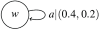



 .



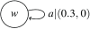




Validity Preservation Over Simulation
This section addresses another question relevant for the characterization of the proposed logic: the preservation of modal validity over different forms of simulation in paraconsistent models. We start with the crisp case.
Theorem 4.
Let
 $M=\langle W,R,V\rangle$
and
 $M'=\langle W',R',V' \rangle$
be two paraconsistent models over a iMTL-algebra
 $\boldsymbol{A}$
, and
 $S \subseteq W \times W'$
be a crisp simulation. Then, for every
 $(w,w') \in S$
and any sentence
 $\varphi \in \mathsf{Sen}^+(\textrm{Prop},\textrm{Act})$
:
 \begin{equation} (M,w \models \varphi ) \, \preccurlyeq \, (M', w' \models \varphi ) \end{equation}
where
 $\mathsf{Sen}^+(\textrm{Prop},\textrm{Act})$
is the positive fragment of
 $\textrm{P}(\boldsymbol{A})$
.
Proof. The proof is by induction over the structure of sentences.
-
• Case
$\bot$
is trivial, using the definition of
$\models$
$(M,w \models \bot ) \,=\, (0,1) \,= \, (M',w' \models \bot )$
. Thus,
\begin{equation*}(M,w \models \bot ) \, \preccurlyeq \, (M',w' \models \bot )\end{equation*}
-
• For
$p \in \textrm{Prop}$
the result follows from the fact that
$S$
is a simulation hence,
$V(w,p)\,\preccurlyeq \, V'(w',p)$
, using the definition of
$\models$
,
$(M,w \models p) \, \preccurlyeq \, (M',w'\models p)$
. -
• For
$\varphi _1 \land \varphi _2$
we reason,
\begin{align*} & (M,w \models \varphi _1 \land \varphi _2) \\ =\; & \scriptstyle {\{\text{defn of }\models \}} \\ & (M,w \models \varphi _1) \mathrel {\substack {\land \\ \land }} (M,w \models \varphi _2)\\ \preccurlyeq \; & \scriptstyle {\{\text{Induction Hypothesis twice}\}} \\ & (M',w' \models \varphi _1) \mathrel {\substack {\land \\ \land }} (M',w' \models \varphi _2)\\ =\; & \scriptstyle {\{\text{defn of }\models \}} \\ & (M',w' \models \varphi _1 \land \varphi _2) \end{align*}
-
• For
$\langle a \rangle \varphi$
,The step labeled by
\begin{align*} & M,w \models \langle a \rangle \varphi \\ =\; & \scriptstyle {\{\text{defn of }\models \}} \\ & \underset {v \in W}{\mathrel {\substack {\lor \\ \lor }}} \, \bigg ( R_a(w,v) \otimes (M,v \models \varphi ) \bigg ) \\ \preccurlyeq \; & \scriptstyle {\{\star \}} \\ & \underset {v' \in W'}{\mathrel {\substack {\lor \\ \lor }}} \, \bigg ( R'_a(w',v') \otimes (M',v' \models \varphi ) \bigg ) \\ =\; & \scriptstyle {\{\text{defn of }\models \}} \\ & M',w' \models \langle a \rangle \varphi \\ \end{align*}
$*$
in the last proof, is justied as follows: since
$S$
is a simulation, there exists
$v' \in W'$
such that
$R_a(w,v) \, \preccurlyeq \, R'_a(w',v')$
and by hypothesis
$(M,v \models \varphi ) \, \preccurlyeq \, (M',v' \models \varphi )$
. Using (19),Since
\begin{equation*}R_a(w,v) \otimes (M,v \models \varphi ) \; \preccurlyeq \; R'_a(w',v') \otimes (M',v' \models \varphi )\end{equation*}
$\mathrel {\substack {\lor \\ \lor }}$
is monotone, we conclude that,
\begin{equation*}\underset {v \in W}{\mathrel {\substack {\lor \\ \lor }}} \, \bigg ( R_a(w,v) \otimes (M,v \models \varphi ) \bigg ) \; \preccurlyeq \; \underset {v' \in W'}{\mathrel {\substack {\lor \\ \lor }}} \, \bigg ( R'_a(w',v') \otimes (M',v' \models \varphi ) \bigg ) \end{equation*}














Not all sentences are, however, preserved by a crisp simulation. Typical examples are
 $\neg \varphi ,\, \varphi _1 \triangleright \varphi _2$
and
 $[a]\varphi$
, as shown by the following counterexamples. Consider the following paraconsistent models
 $M=\langle W,R,V\rangle$
and
 $M'=\langle W',R',V' \rangle$
.
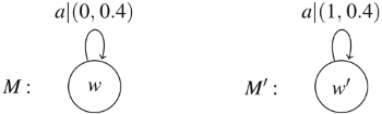
where
 $R_a(w,w)\preccurlyeq R'_a(w',w')$
and
 $V(w,p)=(0.3,0.8) \preccurlyeq (0.6,0.7) =V'(w',p)$
and
 $V(w,q)=(0.1,0.4)\, \preccurlyeq \,(0.2,0.4) =V'(w',q)$
. Hence,
 $S=\{(w,w')\}$
is a simulation.
-
• For
$\neg p$
we have that
$(M,w \models \neg p) = \mathbin {/\mkern -6mu/} V(w,p) =(0.8,0.3)$
and
$(M',w' \models \neg p) = \mathbin {/\mkern -6mu/} V'(w',p) =(0.7,0.6)$
. That is,
-
• For
$p \triangleright q$
we have that
$(M,w \models p \triangleright q)^-= 0.3$
and
$(M',w' \models p \triangleright q)^-=0.4$
. Thus,
-
• For
$[a]p$
, we have that
$(M,w \models [a] p)^-\,=\,0$
and
$(M',w' \models [a] p)^-\,=\,0.7$
. Thus,












Theorem 5.
Let
 $M=\langle W,R,V\rangle$
and
 $M'=\langle W',R',V' \rangle$
be two paraconsistent models over a iMTL-algebra
 $\boldsymbol{A}$
and
 $S^G: W \times W' \rightarrow A \times A$
be a graded simulation. Then, for every
 $w \in W$
,
 $w' \in W'$
and any sentence
 $\varphi \in \mathsf{Sen}^+(\textrm{Prop},\textrm{Act})$
:
 \begin{equation} S^G(w,w') \,\preccurlyeq \, \bigg ( (M,w \models \varphi ) \Rightarrow (M', w' \models \varphi ) \bigg ) \end{equation}
where
 $\mathsf{Sen}^+(\textrm{Prop},\textrm{Act})$
is the positive fragment of
 $\textrm{P}(\boldsymbol{A})$
.
Proof. The proof is by induction over the structure of sentences.
-
• Case
$\bot$
is trivial. By definition of
$\models$
and
$\Rightarrow$
and, since
\begin{equation*}(M,w \models \bot ) \Rightarrow (M',w' \models \bot )\,=\,(0,1) \Rightarrow (0,1)\,=\,(1,0) \end{equation*}
$S^G(w,w') \in A \times A$
we have that
$S^G(w,w') \,\preccurlyeq \,(1,0)$
.
-
• For
$p \in \textrm{Prop}$
, recall that
$S^G$
is a graded simulation and therefore satisfies condition (31). That is,Using the definition of
\begin{equation*}S^G(w,w') \, \preccurlyeq \, V(w,p) \Rightarrow V'(w',p)\end{equation*}
$\models$
\begin{equation*}S^G \, \preccurlyeq \, (M,w \models p) \Rightarrow (M',w' \models p)\end{equation*}
-
• For
$\varphi _1 \land \varphi _2$
(where
$\varphi _1, \,\varphi _2 \in \mathsf{Sen}^+(\textrm{Prop},\textrm{Act})$
) the proof is as follows:
\begin{align*} & (M,w \models \varphi _1 \land \varphi _2) \Rightarrow (M',w' \models \varphi _1 \land \varphi _2) \\ =\; & \scriptstyle {\{\text{defn }\models \}} \\ & ( M,w \models \varphi _1 \, \mathrel {\substack {\land \\ \land }}\, M,w \models \varphi _2) \, \Rightarrow \, ( M',w' \models \varphi _1 \, \mathrel {\substack {\land \\ \land }} \, M',w' \models \varphi _2) \\ \succcurlyeq \; & \scriptstyle {\{\text{Property (30)}\}} \\ &( M,w \models \varphi _1 \Rightarrow M',w' \models \varphi _1) \mathrel {\substack {\land \\ \land }} ( M,w \models \varphi _2 \Rightarrow M',w' \models \varphi _2) \\ \succcurlyeq \; & \scriptstyle {\{\text{Induction hypothesis and }\mathrel {\substack {\land \\ \land }}\text{ is idempotent}\}} \\ & S^G(w,w') \end{align*}
-
• For
$\langle a \rangle \varphi$
, consider, without loss of generality, a state
$v \in W$
such that(40)Since
\begin{equation} (M,w \models \langle a \rangle \varphi ) \, =\, R_a(w,v) \otimes M,v \models \varphi \end{equation}
$S^G$
is a graded simulation, by (32) there is
$v' \in W'$
such that the following inequality is satisfied.(41)We will prove that,
\begin{equation} S^G (w,w') \, \otimes R_a(w,v) \, \preccurlyeq \, R'_a(w',v') \otimes S^G(v,v') \end{equation}
(42)Observe that,
\begin{equation} S^G(w,w') \, \preccurlyeq \, (M,w \models \langle a \rangle \varphi ) \Rightarrow (R'_a(w',v') \otimes M',v' \models \varphi ) \end{equation}
(43)Thus, by proving (42) resorting to property (18), we prove the case
\begin{equation} (R'_a(w',v') \otimes M',v' \models \varphi )\, \preccurlyeq \, (M',w' \models \langle a \rangle \varphi ) \end{equation}
$\langle a \rangle \varphi$
. Since
$S^G$
is a graded simulation,
$S^G(v,v') \, \preccurlyeq \, (M,v \models \varphi ) \Rightarrow (M',v' \models \varphi )$
through (18) in (41),Using Property (17),
\begin{equation*}S^G(w,w') \otimes R_a(w,v) \, \preccurlyeq \, R'_a(w',v') \otimes ((M,v \models \varphi ) \Rightarrow (M',v' \models \varphi ))\end{equation*}
Using Property (23),
\begin{equation*} S^G(w,w') \, \preccurlyeq \, R_a(w,v) \Rightarrow \bigg (R'_a(w',v') \otimes ((M,v \models \varphi ) \Rightarrow (M',v' \models \varphi ))\bigg ) \end{equation*}
Using Property (24)
\begin{equation*} S^G(w,w') \, \preccurlyeq \, R_a(w,v) \Rightarrow \bigg ((M,v \models \varphi ) \Rightarrow ( R'_a(w',v') \otimes (M',v' \models \varphi ))\bigg ) \end{equation*}
Given (40), (43) and (18), we conclude that
\begin{equation*} S^G(w,w') \, \preccurlyeq \, \bigg ( R_a(w,v) \otimes (M,v \models \varphi ) \bigg ) \Rightarrow \bigg (R'_a(w',v') \otimes (M',v' \models \varphi )\bigg ) \end{equation*}
\begin{equation*}S^G(w,w') \, \preccurlyeq \, ( M,w \models \langle a \rangle \varphi ) \Rightarrow (M',w' \models \langle a \rangle \varphi ) \end{equation*}












Again some formulas are not preserved by a graded simulation. Such are the cases of
 $\neg \varphi$
,
 $\varphi _1 \triangleright \varphi _2$
,
 $[a]\varphi$
. Counterexamples are provided below for each case.
-
• For
$\neg \varphi$
consider the following paraconsistent models
with
$V(w,p)=(0,0.3)$
and
$V'(w',p)=(0.3,0)$
. Relation
$S^G(w,w') \, =\, (1,0)$
is a graded simulation, since it satisfies conditions (31) and (32). Note that,However,
\begin{equation*}(M,w \models \neg p) \Rightarrow (M',w' \models \neg p) \,=\, (0.3,0) \Rightarrow (0,0.3)\,=\, (0,0.3) \end{equation*}
. -
• For
$\varphi _1 \triangleright \varphi _2$
consider again the above paraconsistent models now with
$V(w,p)\,=\,V(w,q) \,=\,(0.5,0.5)$
and
$V'(w',p)\,=\,(1,0.5)$
and
$V'(w',q)\,=\,(0.5,1)$
. Relation
$S^G(w,w') \,=\, (1,0.5)$
is a graded simulation. Note that,However,
\begin{align*} &(M,w \models p \triangleright q ) \Rightarrow (M',w' \models p \triangleright q) \\ =\; & \mathbin {/\mkern -6mu/} \bigg ( (M,w \models p) \mathrel {\substack {\land \\ \land }} \mathbin {/\mkern -6mu/} (M,w \models q) \bigg ) \Rightarrow \mathbin {/\mkern -6mu/} \bigg ( (M',w' \models p) \mathrel {\substack {\land \\ \land }} \mathbin {/\mkern -6mu/} (M',w' \models q) \bigg ) \\ =\; & \mathbin {/\mkern -6mu/} \bigg ( (0.5,0.5) \mathrel {\substack {\land \\ \land }} (0.5,0.5) \bigg ) \Rightarrow \mathbin {/\mkern -6mu/} \bigg ( (1,0.5) \mathrel {\substack {\land \\ \land }} (1,0.5) \bigg )\\ =\; & (0.5,0.5) \Rightarrow (0.5,1) \\ =\; & (0.5,0.5) \end{align*}
. -
• Finally, for
$[a]\varphi$
consider the following two paraconsistent models
with
$V(w,p)\,=\, V'(w',p)\,=\,(1,0)$
,
$V(v,p)\,=\,(0.7,0.6)$
and
$V'(v',p)\,=\, (0.1,0.1)$
. Relation
$S^G(w,w')\,=\,(1,0.1)$
and
$S^G(v,v')\,=\,(0.1,0.1)$
is a graded simulation. Note that,However,
\begin{align*} (M,w \models [a]p ) \Rightarrow (M',w' \models [a] p) =\; & (M,w \models \neg \langle a \rangle \neg p) \Rightarrow (M',w' \models \neg \langle a \rangle \neg p) \\ =\; & \mathbin {/\mkern -6mu/} (M,w \models \langle a \rangle \neg p) \Rightarrow \mathbin {/\mkern -6mu/} (M',w' \models \langle a \rangle \neg p) \\ =\; & \mathbin {/\mkern -6mu/} (R_a(w,v) \otimes \mathbin {/\mkern -6mu/} V(v,p)) \Rightarrow \mathbin {/\mkern -6mu/} (R'_a(w',v') \otimes \mathbin {/\mkern -6mu/} V'(v',p)) \\ =\; & (1,0.1) \Rightarrow (0.1,0.1) \\ =\; & (0.1,0.1) \end{align*}
.






 .






 .

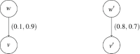






 .
Another interesting observation is that a disjunctive sentence
 $\varphi _1 \lor \varphi _2$
is preserved by graded simulations, eventhough it is defined in terms of
 $\neg$
and
 $\land$
, with
 $\neg$
is not preserved. Let us start by showing that,
 \begin{equation} (M,w \models \varphi _1 \lor \varphi _2 ) \,=\, (M,w \models \varphi _1) \mathrel {\substack {\lor \\ \lor }} (M,w \models \varphi _2) \end{equation}
Let
 $(M,w \models \varphi _1)\,=\, (\alpha , \beta )$
and
 $(M',w' \models \varphi _2)\,=\, (\alpha ', \beta ')$
with
 $\alpha , \,\alpha ', \, \beta , \, \beta ' \in A$
.
 \begin{align*} M,w \models \varphi _1 \lor \varphi _2 \; =\; & M,w \models \neg (\neg \varphi _1 \land \neg \varphi _2) \\ =\; & \mathbin {/\mkern -6mu/} (M,w \models \neg \varphi _1 \land \neg \varphi _2) \\ =\; & \mathbin {/\mkern -6mu/} ( \mathbin {/\mkern -6mu/} (M,w \models \varphi _1) \mathrel {\substack {\land \\ \land }} \mathbin {/\mkern -6mu/} (M,w \models \varphi _2)) \\ =\; & \mathbin {/\mkern -6mu/} ( (\beta , \alpha ) \mathrel {\substack {\land \\ \land }} (\beta ', \alpha ')) \\ =\; & \mathbin {/\mkern -6mu/} (\beta \land \beta ', \alpha \lor \alpha ') \\ =\;& (\alpha \lor \alpha ', \beta \land \beta ')\\ =\; & (M,w \models \varphi _1) \mathrel {\substack {\lor \\ \lor }} (M,w \models \varphi _2) \end{align*}
Thus, the proof of Theorem5 for
 $\varphi _1 \lor \varphi _2$
can be written as follows
 \begin{align*} & (M,w \models \varphi _1 \lor \varphi _2) \Rightarrow (M',w' \models \varphi _1 \lor \varphi _2) \\ =\; & \scriptstyle {\{\text{(44)}\}} \\ & \bigg ( (M, w \models \varphi _1) \mathrel {\substack {\lor \\ \lor }} (M, w \models \varphi _2) \bigg ) \Rightarrow \bigg ( (M', w' \models \varphi _1) \mathrel {\substack {\lor \\ \lor }} (M', w' \models \varphi _2) \bigg ) \\ \succcurlyeq \; & \scriptstyle {\{\text{(29)}\}} \\ & \bigg ((M, w \models \varphi _1) \Rightarrow (M',w' \models \varphi _1)\bigg ) \mathrel {\substack {\land \\ \land }} \bigg ( (M, w \models \varphi _2) \Rightarrow (M',w' \models \varphi _2)\bigg ) \\ \succcurlyeq \; & \scriptstyle {\{\text{Induction hypothesis and $\mathrel {\substack {\land \\ \land }}$ idempotent}\}} \\ & S^G(w,w') \end{align*}
Modal Invariance
Finally, modal invariance is discussed with respect to both crisp and graded bisimulation.
Theorem 6.
Let
 $M=\langle W,R,V\rangle$
,
 $M'=\langle W',R',V' \rangle$
be two paraconsistent models over a iMTL-algebra
 $\boldsymbol{A}$
, and
 $B \subseteq W \times W'$
be a crisp bisimulation. Then, for every
 $(w,w') \in B$
and any sentence
 $\varphi \in \mathsf{Sen}(\textrm{Prop},\textrm{Act})$
,
 \begin{equation} (M,w \models \varphi ) \, = \, (M', w' \models \varphi ) \end{equation}
Proof. The proof is by induction over the structure of sentences.
-
• The case
$\bot$
is trivial from the definition of
$\models$
,
$(M,w \models \bot ) \,=\, (0,1)\, =\, (M',w' \models \bot )$
. -
• For
$p \in \textrm{Prop}$
, since
$B$
is a crisp bisimulation, it follows that
$V(w,p)\,=\,V'(w',p)$
, and by definition of
$\models$
, conclude
$(M,w \models p) \, =\, (M',w' \models p)$
. -
• For
$\varphi _1 \land \varphi _2$
the proof is as follows,
\begin{align*} & M, w \models \varphi _1 \land \varphi _2 \\ =\; & \scriptstyle {\{\text{defn of }\models \}} \\ & ( M, w \models \varphi _1 ) \mathrel {\substack {\land \\ \land }} ( M, w \models \varphi _2)\\ =\; & \scriptstyle {\{\text{Induction Hypothesis twice}\}} \\ & (M', w' \models \varphi _1 ) \mathrel {\substack {\land \\ \land }} (M', w' \models \varphi _2 )\\ =\; & \scriptstyle {\{\text{defn of }\models \}} \\ & M', w' \models \varphi _1 \land \varphi _2\\ \end{align*}
-
• For
$\langle a \rangle \varphi$
,Step (
\begin{align*} & M,w \models \langle a \rangle \varphi \\ =\; & \scriptstyle {\{\text{defn of }\models \}} \\ & \underset {v \in W}{\mathrel {\substack {\lor \\ \lor }}} \, \bigg ( R_a(w,v) \otimes (M,v \models \varphi ) \bigg ) \\ = \; & \scriptstyle {\{\text{($\star \star $)}\}} \\ & \underset {v' \in W'}{\mathrel {\substack {\lor \\ \lor }}} \, \bigg ( R'_a(w',v') \otimes (M',v' \models \varphi ) \bigg ) \\ =\; & \scriptstyle {\{\text{defn of }\models \}} \\ & M',w' \models \langle a \rangle \varphi \\ \end{align*}
$\star \star$
) is proved as follows:
$B$
being a bisimulation, there exists
$v \in W$
such that
$R'_a(w',v') \, =\, R_a(w,v)$
and, by hypothesis,
$(M',v' \models \varphi ) \, = \, (M,v \models \varphi )$
. Therefore,Since
\begin{equation*}R'_a(w',v') \otimes (M',v' \models \varphi ) \, = \, R_a(w,v) \otimes (M,v \models \varphi )\end{equation*}
$\mathrel {\substack {\lor \\ \lor }}$
is monotone,
$\underset {v' \in W'}{\mathrel {\substack {\lor \\ \lor }}} \, \bigg ( R'_a(w',v') \otimes (M',v' \models \varphi ) \bigg ) \, = \, \underset {v \in W}{\mathrel {\substack {\lor \\ \lor }}} \, \bigg ( R_a(w,v) \otimes (M,v \models \varphi ) \bigg )$















Theorem 7.
Let
 $M=\langle W,R,V\rangle$
and
 $M'=\langle W',R',V' \rangle$
be two paraconsistent models over a iMTL-algebra
 $\boldsymbol{A}$
, and
 $B^G: W \times W' \rightarrow A \times A$
be a graded bisimulation. Then, for every
 $w \in W$
,
 $w' \in W'$
and any sentence
 $\varphi \in \mathsf{Sen}(\textrm{Prop},\textrm{Act})$
,
 \begin{equation} B^G(w,w') \,\preccurlyeq \, \bigg ( (M,w \models \varphi ) \Leftrightarrow (M', w' \models \varphi ) \bigg ) \end{equation}
Proof. The proof is again by induction over the structure of sentences.
-
• Case
$\bot$
is trivial,
\begin{equation*}B^G(w,w') \,\preccurlyeq \, (M,w \models \bot ) \Leftrightarrow (M',w' \models \bot )\,=\,(0,1) \Leftrightarrow (0,1)\,=\,(1,0) \end{equation*}
-
• For
$p\in \textrm{Prop}$
, since
$B^G$
is a graded bisimulation it satisfies condition (33), that isUsing the definition of
\begin{equation*}B^G(w,w') \, \preccurlyeq \, V(w,p) \Leftrightarrow V'(w',p)\end{equation*}
$\models$
, we conclude
\begin{equation*}B^G \, \preccurlyeq \, (M,w \models p) \Leftrightarrow (M',w' \models p)\end{equation*}
-
• For
$\neg \varphi$
,
\begin{align*} & (M,w \models \neg \varphi ) \Leftrightarrow (M,w \models \neg \varphi ) \\ =\; & \scriptstyle {\{\text{defn of }\models \}} \\ & \mathbin {/\mkern -6mu/}(M,w \models \varphi ) \Leftrightarrow \mathbin {/\mkern -6mu/}(M,w \models \varphi )\\ =\; & \scriptstyle {\{\text{Property (20)}\}} \\ &(M,w \models \varphi ) \Leftrightarrow (M,w \models \varphi )\\ \succcurlyeq \; & \scriptstyle {\{\text{Induction hypothesis}\}} \\ & B^G(w,w') \end{align*}
-
• For
$\varphi _1 \land \varphi _2$
,
\begin{align*} & \bigg ( (M, w \models \varphi _1) \mathrel {\substack {\land \\ \land }} (M, w \models \varphi _2) \bigg ) \Leftrightarrow \bigg ( (M', w' \models \varphi _1) \mathrel {\substack {\land \\ \land }} (M', w' \models \varphi _2) \bigg ) \\ \succcurlyeq \; & \scriptstyle {\{\text{(27)}\}} \\ & \bigg ((M, w \models \varphi _1) \Leftrightarrow (M',w' \models \varphi _1)\bigg ) \mathrel {\substack {\land \\ \land }} \bigg ( (M, w \models \varphi _2) \Leftrightarrow (M',w' \models \varphi _2)\bigg ) \\ \succcurlyeq \; & \scriptstyle {\{\text{induction hypothesis and $\mathrel {\substack {\land \\ \land }}$ idempotent}\}} \\ & B^G(w,w') \end{align*}
-
• For
$\langle a \rangle \varphi$
we need to verify the following two inequalities,(47)
\begin{align} & B^G(w,w') \, \preccurlyeq \, (M,w \models \langle a \rangle \varphi ) \Rightarrow (M',w'\models \langle a \rangle \varphi ) \end{align}
(48)
\begin{align} & B^G(w,w') \, \preccurlyeq \, (M',w' \models \langle a \rangle \varphi ) \Rightarrow (M,w\models \langle a \rangle \varphi ) \end{align}
The proof for (47) is equal to the one presented for case
$\langle a \rangle \varphi$
in Theorem5. Similarly, one can prove (48). Since
$B^G$
is a graded bisimulation, there is
$v \in W$
such that the following inequality is satisfied(49)We will prove that for
\begin{equation} B^G(w,w') \otimes R'_a(w',v') \, \preccurlyeq \, R_a(w,v) \otimes B^G(v,v') \end{equation}
$v \in W$
,(50)Observe that,
\begin{equation} B^G(w,w') \, \preccurlyeq \, (M',w' \models \langle a \rangle \varphi ) \Rightarrow (R_a(w,v) \otimes M,v \models \varphi ) \end{equation}
(51)Thus, by proving (50) using property (18), we verify (48). Since
\begin{equation} (R_a(w,v) \otimes M,v \models \varphi )\, \preccurlyeq \, (M,w \models \langle a \rangle \varphi ) \end{equation}
$B^G$
is a graded simulation,
$B^G(v,v') \, \preccurlyeq \, (M',v' \models \varphi ) \Rightarrow (M,v \models \varphi )$
. Using (18) in (49), entailsThen, by (17),
\begin{equation*}B^G(w,w') \otimes R'_a(w',v') \, \preccurlyeq \, R_a(w,v) \otimes ((M',v' \models \varphi ) \Rightarrow (M,v \models \varphi ))\end{equation*}
Using (23),
\begin{equation*} B^G(w,w') \, \preccurlyeq \, R'_a(w',v') \Rightarrow \bigg (R_a(w,v) \otimes ((M',v' \models \varphi ) \Rightarrow (M,v \models \varphi ))\bigg ) \end{equation*}
Using (24),
\begin{equation*} B^G(w,w') \, \preccurlyeq \, R'_a(w',v') \Rightarrow \bigg ((M',v' \models \varphi ) \Rightarrow ( R_a(w,v) \otimes (M,v \models \varphi ))\bigg ) \end{equation*}
By (18),
\begin{equation*} B^G(w,w') \, \preccurlyeq \, \bigg ( R'_a(w',v') \otimes (M',v' \models \varphi ) \bigg ) \Rightarrow \bigg (R_a(w,v) \otimes (M,v \models \varphi )\bigg ) \end{equation*}
Finally, by (47) and (48) and the fact that
\begin{equation*}B^G(w,w') \, \preccurlyeq \, ( M',w' \models \langle a \rangle \varphi ) \Rightarrow (M,w \models \langle a \rangle \varphi ) \end{equation*}
$\mathrel {\substack {\land \\ \land }}$
is monotone,
\begin{equation*}B^G(w,w') \, \preccurlyeq \, (M,w \models \langle a \rangle \varphi )\Leftrightarrow (M',w' \models \langle a \rangle \varphi )\end{equation*}





6. An Application to Robotics
In this section, we take the initial steps toward exploring a potential application of paraconsistent transition systems in robotics. This inspiration is drawn from the work documented in Abe et al. (Reference Abe, Torres, Lambert-Torres, da Silva Filho, Martins, Lambert-Torres, Abe, da Silva Filho and Martins2007) and its adaptation in Costa and Martins (Reference Costa and Martins2016), where paraconsistent logics are employed to determine the movements of a robot. The main goal is to investigate how the robot, which may receive contradictory information regarding the presence (or absence) of objects in its environment, navigates along a specific path.
While sensors for object detection remain internally consistent, discrepancies may arise between them, particularly if their methods for object detection are different. Furthermore, sensors are susceptible to contradictions due to various factors, such as hardware limitations that restrict the accuracy in measuring to a certain degree, and the fact that measurements themselves can be affected by outside conditions. Consequently, it is not uncommon information collected by one sensor to contradict that collected by another. On the other hand, combining various types of sensors is a common practice to enhance reliability and accuracy in obstacle detection and avoidance.
These challenges motivate our approach to incorporate various types of sensors, consider external conditions and use each sensor’s characteristics in determining confidence in object detection along different navigation paths. To illustrate this, let us work with 4 sensors: two ultrasonic sensors that measure distance to an obstacle by using ultrasonic waves, and two infrared reflective sensors that detect the presence of an obstacle by measuring the amount of reflected infrared light. There will be two sets of sensors: one called the set of “positive sensors” that comprises one sensor of each type (one ultrasonic and one infrared), while the other is called the set “of negative sensors” and includes the remaining sensors of each type. Both sets of sensors evaluate if a path is free of obstacles or not. Then each set provides a value in the interval
 $[0,1]$
. Such value represents, for the “positive sensors”, its certainty that there is no obstacle and the path is clear, while for the “negative sensors” it represents its certainty that there is an obstacle and the path is obstructed.
Certainty is a crucial aspect in object detection, where the system not only identifies objects but also quantifies its confidence in the accuracy of identification. Various approaches can be adopted to measure certainty, such as considering limitations in the precision of measurements, disregarding a sensor’s output in the presence of environmental conditions that affect measurements, and setting different threshold levels for activation and deactivation to maintain stability in the output due to noise or minor fluctuations.
It is also possible to take into consideration different placements of the sensors. For instance, in Costa and Martins (Reference Costa and Martins2016), the approach involved a robot with two sensors covering a total amplitude of 180
 $^{\circ }$
: one on the left covering 90
 $^{\circ }$
to the left, and the other on the right covering 90
 $^{\circ }$
to the right, as illustrated in Figure 2. Thus, at specific points along the path certain sensors may be temporarily disregarded or have default values adopted to increase confidence in detection.
The angles of vision of each sensor of the robot (Costa and Martins Reference Costa and Martins2016).

In our example, the robot is capable of movement in four directions (left, right, up, and down) and is equipped with two sets of different types of sensors. To simplify the problem, as the robot navigates through a map with four checkpoints, a condition is imposed that prohibits the robot to return to a previously visited checkpoint (resulting in paths with maximum length of 3). We will also assume a non adaptive approach since we will only focus on walks that have one or two moves. However, it is possible to consider that at each state the robot has more information, and makes decisions based on them. The checkpoints are represented by states in a paraconsistent model and transitions between these states represent the robot’s movement from one checkpoint to another. The transition labels indicate the information given by the set of “positive sensors” and the “negative sensors” to move in that direction. Thus, each path will entail a pair
 $(\alpha , \beta )$
, where
 $\alpha$
indicates the certainty degree up to which the “positive sensors” detected the path is clear, and
 $\beta$
indicates the certainty degree up to which the “negative sensors” detected the path is obstructed.
As before, for any given pair
 $(\alpha , \beta )$
, if
 $\alpha + \beta = 1$
, we face a scenario where all sensors are consistent with each other, if
 $\alpha + \beta \lt 1$
, the sensors are consistent but lack sufficient information together to draw a conclusion and if
 $\alpha + \beta \gt 1$
, the sensors disagree with each other. For example, a label such as
-
(1)
$(1,0)$
indicates complete agreement between all of the sensors that the path is clear, allowing the robot to move freely in that direction; -
(2)
$(0,1)$
indicates unanimous consensus between all of the sensors that the path is not clear, restricting the robot from moving in that direction; -
(3)
$(1,1)$
suggests complete disagreement between both sensors, leading to the paradoxical situation where they are simultaneously certain that the path is clear and not clear. -
(4)
$(0,0)$
reflects minimal certainty from both sensors regarding the path’s status as free or obstructed.


Scenarios of inconsistency, as in 3, or vagueness, as in 4, may be more challenging to picture than others. However, it is conceivable that under external unfavorable conditions, such as adverse weather, sensors could either demonstrate complete disagreement or lack confidence in their measurements.
Additionally, the proposition
 $Obst$
serves as a crisp valuation indicating the presence of an obstacle at a given state, with a valuation of
 $(1,0)$
, or the absence of an obstacle, with a valuation of
 $(0,1)$
.
Let us consider the following map:
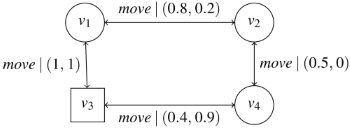
If the robot is initially positioned in state
 $v_1$
, the path to
 $v_2$
is reportedly clear by the “positive sensors” with a certainty of
 $0.8$
, and it is reported as not clear by the “negative sensors” with a certainty of
 $0.2$
. The only state that contains an obstacle is state
 $v_3$
and therefore is pictured differently in the model.
Let us evaluate a few sentences and explore the robot’s behavior in the paraconsistent model.

-
• The sentence
$ Obst \rightarrow [move] \bot$
indicates that whenever a state has an obstacle, the robot should not be able to move. As expected, this sentence at states
$v_1,\,v_2$
and
$v_4$
is consistently true since they do not have obstacles. However, at state
$v_3$
the evaluation is consistently false. Eventhough, state
$v_3$
has an obstacle, there is positive evidence that it is possible to move to another state.The problem arises because both
\begin{align*} & M,v_3 \models Obst \rightarrow [move] \bot \\ =&\ M,v_3 \models Obst \rightarrow \neg \langle move \rangle \, \top \\ =&\ M,v_3 \models \neg \,( Obst \land \langle move \rangle \, \top ) \\ =& \mathbin {/\mkern -6mu/} \, \bigg ( (M,v_3 \models Obst) \, \mathrel {\substack {\land \\ \land }} \,(M,v_3 \models \langle move \rangle \top ) \bigg ) \\ =& \mathbin {/\mkern -6mu/} \, \bigg ( V(v_3,Obst) \, \mathrel {\substack {\land \\ \land }} \,((R_{move}(v_3,v_1) \otimes (1,0)) \mathrel {\substack {\lor \\ \lor }} ( R_{move}(v_3,v_4) \otimes (1,0)) \bigg ) \\ =& \mathbin {/\mkern -6mu/} \, \bigg ((1,0) \, \mathrel {\substack {\land \\ \land }} \,( (1,0) \mathrel {\substack {\lor \\ \lor }} (0.4,0) \bigg ) \\ =&\ (0,1) \end{align*}
$R^+_{move}(v_3,v_1)$
and
$R^+_{move}(v_3,v_4)$
are both different from
$0$
. If, at that state, external and internal conditions for the sensors were improved to the extent that the positive sensors indicate the path is clear with
$0$
certainty, and the negative sensors report the path is obstructed with the same certainty level, that is,
$R_{move}(v_3,v_1)=(0,1)$
and
$R_{move}(v_3,v_4)=(0,0.9)$
. Then,Only with such changes would the robot’s behavior at that state align with the expected result, that is, the robot at state
\begin{align*} & M,v_3 \models Obst \rightarrow [move] \bot \\ =& \mathbin {/\mkern -6mu/} \, \bigg ( (M,v_3 \models Obst) \, \mathrel {\substack {\land \\ \land }} \,(M,v_3 \models \langle move \rangle \top ) \bigg ) \\ =& \mathbin {/\mkern -6mu/} \, \bigg ( V(v_3,Obst) \, \mathrel {\substack {\land \\ \land }} \,((R_{move}(v_3,v_1) \otimes (1,0)) \mathrel {\substack {\lor \\ \lor }} ( R_{move}(v_3,v_4) \otimes (1,0)) \bigg ) \\ =& \mathbin {/\mkern -6mu/} \, \bigg ( V(v_3,Obst) \, \mathrel {\substack {\land \\ \land }} \,( ((0,1) \otimes (1,0)) \mathrel {\substack {\lor \\ \lor }} ( (0,0.9) \otimes (1,0)) \bigg ) \\ =& \mathbin {/\mkern -6mu/} \, \bigg ((1,0) \, \mathrel {\substack {\land \\ \land }} \,( (0,1) \mathrel {\substack {\lor \\ \lor }} (0,0.9) \bigg ) \\ =&\ (0.9,0) \end{align*}
$v_3$
has (almost) complete certainty that in the presence of an obstacle, it cannot move.
-
• The sentence
$\neg Obst \land \langle move \rangle \neg Obs$
indicates that at a state with no obstacle it is possible to move to another state where there is still no obstacle. At state
$v_4$
, there is less positive certainty of movement than at states
$v_1$
and
$v_2$
. Thus, the evaluation of the sentence at
$v_4$
is
$(0.5,0)$
, while at
$v_1$
and
$v_2$
it is
$(0.8,0)$
. Given that
$(0.5,0) \preccurlyeq (0.8,0)$
when planning the robot’s path, we might take the starting position at state
$v_1$
instead of
$v_4$
. This is because there is overall more certainty that the first move from state
$v_1$
will not encounter an obstacle. -
• The sentence
$\neg Obst \land \langle move \rangle \neg Obst \land \langle move \rangle \langle move \rangle \neg Obst$
indicates that at a state with no obstacle, it is possible to move two steps without ever encountering an obstacle. This sentence evaluation is consistently false at state
$v_3$
, which has an obstacle, and at state
$v_2$
because every walk that starts at
$v_2$
and takes two steps will always lead to
$v_3$
. Finally, at states
$v_1$
and
$v_4$
, there is a
$0.5$
certainty that taking two steps will lead to a path without obstacles, and there is a
$0$
certainty that taking two steps will encounter an obstacle. This situation represents a vague scenario where the sum of the weights is less than
$1$
. This is because transitions from
$v_1$
to
$v_2$
to
$v_4$
and vice versa always present positive evidence smaller than
$1$
, so they do not have complete certainty that it is possible to move. However, they present
$0$
or close to
$0$
negative evidence that the transitions will be prevented from occurring due to obstacle detection.
















This example shows how paraconsistent models and their logics can be used in practice to model complex, weakly consistent situations, and enabling reasoning about them. It is worth noting that this example can be enhanced by incorporating dynamic operators from dynamic logic extended to the paraconsistent setting, as introduced in our prior work (Cunha et al. Reference Cunha, Madeira, Barbosa, David and Sun2023a). Reference Barbosa and Madeira (Reference Barbosa, Madeira, Chiba, Cong and Boix2023) reports on another application in a totally different domain, that of quantum circuits analysis in the presence of decoherence.
7. Conclusions and Future Work
This paper studied a new kind of labeled transition structures able to capture both vagueness and inconsistency in software modeling scenarios. Two main research directions were pursued. First, the structure of a category of (pointed) PLTS was explored to define a number of useful operators to build such systems in a compositional way. Then, a modal logic, whose modalities are indexed by transition labels, was proposed. Preliminary results of classical and graded soundness were explored. This graded variant adjusts the classical definition of soundness to accommodate vague and inconsistent evaluations. Thus, a rule of the form:
 \begin{equation*} \frac {{\varphi _1\;\ldots \; \varphi _n}}{\varphi } \end{equation*}
is g-sound if for any paraconsistent Kripke model
 $M=\langle W,R,V\rangle$
,
 \begin{equation*}\underset {i=1}{\overset {n}{\mathrel {\substack {\land \\ \land }}}} (M \models \varphi _i) \preccurlyeq \, (M \models \varphi )\end{equation*}
This implies that from the evidence of truth and falsity of premises, it is possible to draw conclusions whose evidence of truth is higher and evidence of falsity is lower. Remarkably, while g-soundness entails classical soundness, the reverse is not true. This lack of equivalence prompts further investigation in § 5.2 of classical and graded soundness in paraconsistent Kripke models.
Current work seeks to develop an axiomatic system and prove its completeness and soundness for the paraconsistent logic discussed. Drawing inspiration from research on many-valued complete logics (Caicedo and Rodríguez Reference Caicedo and Rodríguez2010), we anticipate achieving similar results, at least for the positive component of the paraconsistent logic presented in this paper. Our approach so far has been to separately explore and establish the completeness and soundness of the positive and negative components of the logic, with the aim of later combining them for overall results. This strategy offers greater flexibility, as some statements are theorems in the positive component but not in the negative, indicating that we may be certain that a statement will always hold (positively it is a theorem), but the evidence for it not holding may not be exactly complementary (negatively it is not a theorem); the converse can also occur.
From this ongoing work, preliminary findings include the observation that the inference rule Modus Ponens preserves truth in the positive component, that is, if the premises hold with positive certainty
 $1$
, then the conclusions also hold with positive certainty
 $1$
, but not in the negative component, meaning that premises may have negative certainty, but the conclusions do not necessarily follow. Additionally, we have found that the modal logic is not normal, as it does not include the schema
 $\square (A\to B)\to (\square A \to \square B)$
.
This paper also introduced both crisp and graded notions of simulation and bisimulation of the corresponding (paraconsistent) Kripke models were also characterized and a number of modal preservation results proved. It remains to consider other notions of equivalence from coalgebraic trace equivalence (Urabe and Hasuo Reference Urabe and Hasuo2018) to logic-induced bisimulations (Beohar et al. Reference Beohar, Gurke, König, Messing, Klin and Pimentel2023) and their corresponding preservation results.
A lot remains to be done, namely in what concerns the development of the logic’s proof-theoretic perspective, which is not addressed here. Such is crucial from a Software Engineering point of view, as a major step towards (semi-)automatic support to reasoning about such complex, often weird, but actually quite common phenomena. The development of a proper specification theory Sannella (Reference Sannella2012) is also worth to explore, following some preliminary work by the authors documented in Cunha et al. (Reference Cunha, Madeira, Barbosa, David and Sun2023a,b).
The detailed characterization of different application scenarios, from AI models to quantum computation and robotics, constitutes another main challenge for the future, once the basic mathematical structure has been completely unveiled.
Acknowledgment
This work is supported by the FCT - Portuguese Foundation of Science and Technology with grant 2024.04652.BD and with projects PTDC/CCI-COM/4280/2021, UIDB/04106/2025 and Bansky - A paraconsistent inference engine to support research in age-related macular degeneration.
Appendix A. Proof of Lemma1
We will focus on the proofs of properties (12), (13), (14), and (16). The proofs for the remaining properties can be found in Nguyen (Reference Nguyen2022).
-
• Property (12) is a direct consequence of (1) applied to the trivial assertion
$a\to c \, \leq \, a \to c$
-
• To prove Property (13) we start by proving
(52)and then
\begin{equation} (a \to c) \land (b \to c) \, \leq \, (a \lor b) \to c \end{equation}
(53)Trivially,
\begin{equation} (a \to c) \land (b \to c) \, \geq \, (a \lor b) \to c \end{equation}
$c \, \geq \, c \land (b \to c)$
and
$c \, \geq \, c \land (a \to c)$
and since
$\lor$
is monotone,
$c \, \geq \, (c \land (b \to c)) \lor (c \land (a \to c))$
. Then, Property (12) entails
$c \, \geq \, a \land (a \to c)$
and
$c\, \geq \, b \land (b \to c)$
, leading toas
\begin{equation*}c \, \geq \, (a \land (a \to c) \land (b \to c)) \lor (b \land (b\to c) \land (a \to c))\end{equation*}
$\land$
and
$\lor$
are monotone as well. Since
$\land$
is associative, property (10) entails
$c \, \geq \, (a \lor b) \land ((a \to c) \land (b \to c))$
. Finally, using Property (1) we have (52). To prove (53) we start with the trivial assertions
$a \leq a \lor b$
and
$b \leq a \lor b$
. By Property (5),
$(a \lor b) \to c\,\leq \, a \to c$
and
$(a \lor b) \to c\,\leq \, b \to c$
. Finally, since
$\land$
is monotone and idempotent we prove (53).
-
• To prove property (14) we first start by proving
$(a \to b) \land (a \to c) \, \leq \, a \to (b \land c)$
and then
$ a \to (b \land c) \,\leq \, (a \to b) \land (a \to c)$
. According to property (12),
$a \land (a \to b) \, \leq \, b$
and
$a \land (a \to c) \, \leq \, c$
. Since
$\land$
is monotone and idempotent,
$a \land (a \to b) \land (a \to c) \, \leq \, b \land c$
. Using (1), entails
$(a \to b) \land (a \to c) \, \leq \, a \to (b \land c)$
. Moreover, trivially
$b \land c \leq b$
and
$b \land c \leq c$
by Property (5)
$a \to (b\land c) \, \leq \, a \to b$
and
$a \to (b\land c) \, \leq \, a \to c$
. Finally, given that
$\land$
is monotone and idempotent
$a \to (b \land c) \, \leq \, (a \to b) \land (a \to c)$
-
• To prove property (16), observe that, by (12),
$(b \to c) \land b \, \leq \, c$
. Since
$\land$
is monotone and associative
$b \land a \land (b \to c)\, \leq \, (c \land a)$
. Using (1) it follows that
$a \land (b \to c) \, \leq \, b \to (c \land a)$
.
































Appendix B. Proof of Lemma3
-
• To prove Property (18) we need to prove
$(a \to c) \land (d \to b) \, \leq \, (a' \to c') \land ( d' \to b')$
and
$a \land d \, \geq \, a' \land d'$
. Let us assume that
$a' \leq a$
,
$c \leq c'$
,
$b' \geq b$
and
$d \geq d'$
. By Property (5),
$(a \to c) \, \leq \, (a' \to c')$
and
$(d \to b) \, \leq \, (d' \to b')$
. Since
$\land$
is monotone,
$(a \to c) \land (d \to b) \, \leq \, (a' \to c') \land (d' \to b')$
. Finally, by hypothesis and the fact that
$\land$
is monotone,
$a \land d \, \geq \, a' \land d'$
. -
• To prove Property (19) we need to prove that
$a \land c \, \leq \, a' \land c'$
and that
$(a \to d) \land (c \to b) \, \geq \,(a' \to d') \land (c' \to b')$
. By hypothesis
$a \leq a'$
and
$c \leq c'$
, since
$\land$
is monotone
$a \land c \, \leq \, a' \land c'$
. Also by hypothesis,
$b \geq b'$
and
$d \geq d'$
, by Property (5),
$(a \to d) \land (c \to b) \, \geq \,(a' \to d') \land (c' \to b')$
. -
• To prove Property (20) note that
Since
\begin{align*} &(a,b) \Leftrightarrow (c,d) \, =\, ((a \leftrightarrow c) \land (d \leftrightarrow b), (a \land d) \lor (c \land b))\\ &\mathbin {/\mkern -6mu/} (a,b) \Leftrightarrow \mathbin {/\mkern -6mu/} (c,d) \, = \,(b,a) \Leftrightarrow (d,c) \, =\, ((b \leftrightarrow d) \land (a \leftrightarrow c), (c \land b) \lor (a \land d)) \end{align*}
$\land$
and
$\lor$
are associative, the pair
$(a,b) \Leftrightarrow (c,d)$
is equal to the pair
$\mathbin {/\mkern -6mu/} (a,b) \Leftrightarrow \mathbin {/\mkern -6mu/} (c,d)$
.
-
• To prove Property (21) note that
By Property (10), it follows that
\begin{gather*} (a,b) \otimes ( (c,d) \mathrel {\substack {\lor \\ \lor }} (e,f)) \, =\, ( a \land (c \lor e), a \to (d \land f) \land (c \lor e) \to b) \\ ((a,b) \otimes (c,d) ) \mathrel {\substack {\lor \\ \lor }} ( (a,b) \otimes (e,f) ) \,=\, ((a \land c) \lor (a \land e), a \to d \land c \to b \land a \to f \land e \to b) \end{gather*}
$a \land (c \lor e) \,=\, (a \land c) \lor (a \land e)$
and by Property (13) and (14) it follows
$a \to (d \land f) \land (c \lor e) \to b \,=\, a \to d \land c \to b \land a \to f \land e \to b$
.
-
• To prove Property (22) note that
$(c,d) \mathrel {\substack {\land \\ \land }} (e,f) \,\preccurlyeq \, (c,d)$
and
$(c,d) \mathrel {\substack {\land \\ \land }} (e,f) \,\preccurlyeq \, (e,f)$
. Using Property (19),Finally, since the operator
\begin{align*} \begin{split} (a,b) \otimes \bigg ( (c,d) \mathrel {\substack {\land \\ \land }} (e,f) \bigg ) \,\preccurlyeq \, (a,b) \otimes (c,d) \\ (a,b) \otimes \bigg ( (c,d) \mathrel {\substack {\land \\ \land }} (e,f) \bigg ) \,\preccurlyeq \, (a,b) \otimes (e,f) \end{split} \end{align*}
$\mathrel {\substack {\land \\ \land }}$
is monotone it implies that,
\begin{equation*} (a,b) \otimes \bigg ( (c,d) \mathrel {\substack {\land \\ \land }} (e,f) \bigg ) \, \preccurlyeq \, \bigg ( (a,b) \otimes (c,d) \bigg ) \mathrel {\substack {\land \\ \land }} \bigg ( (a,b) \otimes (e,f) \bigg ) \end{equation*}
-
• To prove Property (23) note that,
Thus, we want to prove
\begin{align*} (a,b) \otimes ( (c,d) \Rightarrow (e,f) ) =\; & (a,b) \otimes ((c \to e) \land (f \to d), c \land f) \\ =\; & ( a \land (c \to e) \land (f \to d), (a \to (c \land f)) \land ((c \to e \land f \to d) \to b))\\ (c,d) \Rightarrow ( (a,b) \otimes (e,f)) =\; & (c,d) \Rightarrow (a \land e, (a \to f) \land (e \to b))\\ =\; & ((c \to (a \land e)) \land (((a \to f) \land (e \to b)) \to d), c \land (a\to f) \land (e \to b)) \end{align*}
(54)
\begin{align}&\,\, \ a \land (c \to e) \land (f \to d) \, \leq \, (c \to (a \land e)) \land ((a \to f \land e \to b) \to d) \end{align}
(55)
\begin{align}& (a \to (c \land f)) \land (((c \to e) \land (f \to d)) \to b) \, \geq \, c \land (a \to f) \land (e \to b) \end{align}
The proof of inequality (54) follows as
For inequality (55) consider
\begin{align*} & a \land (c \to e) \land (f \to d) \\ =\; & \scriptstyle {\{\text{$\land $ is idempotent and associative}\}} \\ & a \land (c \to e) \land a \land (f \to d) \\ \leq \; & \scriptstyle {\{\text{(16)}\}} \\ & (c \to (a \land e)) \land a \land (f \to d) \\ \leq \; & \scriptstyle {\{\text{(15)}\}} \\ & (c \to (a \land e)) \land ((a \to f) \to d) \\ \leq \; & \scriptstyle {\{\text{since $(a \to f) \, \geq \ (a \to f) \land (e \to b)$ and (5)}\}} \\ & (c \to (a \land e)) \land (((a \to f) \land (e \to b)) \to d) \end{align*}
\begin{align*} & (a \to (c \land f)) \land (((c \to e) \land (f \to d)) \to b) \\ \geq \; & \scriptstyle {\{\text{(16)}\}} \\ & c \land (a \to f) \land (((c \to e) \land (f \to d)) \to b) \\ \geq \; & \scriptstyle {\{\text{since $c \to e\, \geq \, (c \to e) \land (f \to d)$ by (5)}\}} \\ & c \land (a \to f) \land ((c \to e) \to b) \\ \geq \; & \scriptstyle {\{\text{(15)}\}} \\ & c \land (a \to f) \land c \land (e \to b) \\ =\; & \scriptstyle {\{\text{$\land $ is idempotent}\}} \\ & c \land (a \to f) \land (e \to b) \end{align*}
-
• To prove Property (24) note that,
Thus, we want to prove that,
\begin{align*} (a,b) \Rightarrow ( (c,d) \Rightarrow (e,f)) =\; & (a,b) \Rightarrow ((c \to e) \land (f \to d), c \land f) \\ =\; & ((a \to ((c \to e) \land (f \to d))) \land ((c \land f) \to b), a \land c \land f) \\ ( (a,b) \otimes (c,d) ) \Rightarrow (e,f) =\; & (a \land c, (a \to d) \land (c \to b)) \Rightarrow (e,f)\\ =\; & ( ((a \land c) \to e) \land (f \to ((a \to d) \land (c \to b))), a \land c \land f) \end{align*}
The proof follows as,
\begin{equation*} (a \to ((c \to e) \land (f \to d))) \land ((c \land f) \to b) \leq \, ((a \land c) \to e) \land (f \to ((a \to d) \land (c \to b))) \end{equation*}
\begin{align*} & (a \to ((c \to e) \land (f \to d))) \land ((c \land f) \to b) \\ \leq \; & \scriptstyle {\{\text{(5), and $\land $ is monotone}\}} \\ & (a \to (c \to e))\land (a \to (f \to d)) \land ((c \land f) \to b) \\ =\; & \scriptstyle {\{\text{(9)}\}} \\ &((a \land c) \to e) \land (a \to (f \to d)) \land ((c \land f) \to b)\\ =\; & \scriptstyle {\{\text{(8)}\}} \\ &((a \land c) \to e) \land (f \to (a \to d)) \land ((c \land f) \to b)\\ =\; & \scriptstyle {\{\text{(9)}\}} \\ & ((a \land c) \to e) \land (f \to (a \to d)) \land (f \to (c \to b))\\ \leq \; & \scriptstyle {\{\text{ (14)}\}} \\ & ((a \land c) \to e) \land (f \to ((a \to d) \land (c \to b))) \\ \end{align*}
-
• To prove Property (25) let us start by noting that,
which entails the need to prove the following inequalities,
\begin{align*} (a,b) \otimes ( (c,d) \Rightarrow (e.f) ) =\; &(a,b) \otimes ((c \to e) \land (f \to d), c \land f)\\ =\; & (a \land (c \to e) \land (f \to d), (a \to (c \land f)) \land (((c \to e)\\& \land (f \to d)) \to b))\\ ( (a,b) \Rightarrow (c,d) ) \Rightarrow (e,f) =\; & ( (a \to c) \land (d \to b), a \land d) \Rightarrow (e,f) \\ =\; & ( (((a\to c) \land (d \to b)) \to e) \land (f \to (a \land d)), (a \to c) \\&\land (d \to b) \land f) \end{align*}
(56)
\begin{align} a \land (c \to e) \land (f \to d) \, \leq \, (((a\to c) \land (d \to b)) \to e) \land (f \to (a \land d)) \end{align}
(57)
\begin{align} (a \to (c \land f)) \land (((c \to e) \land (f \to d)) \to b) \, \geq \, (a \to c) \land (d \to b) \land f \end{align}
Thus, for (56),
and, for (57),
\begin{align*} & a \land (c \to e) \land (f \to d) \\ =\; & \scriptstyle {\{\text{$\land $ is idempotent and associative}\}} \\ & a \land (c \to e) \land a \land (f \to d) \\ \leq \; & \scriptstyle {\{\text{(15)}\}} \\ & ((a \to c) \to e) \land a \land (f \to d) \\ \leq \; & \scriptstyle {\{\text{(5)}\}} \\ & (((a \to c) \land (d \to b)) \to e) \land a \land (f \to d) \\ \leq \; & \scriptstyle {\{\text{(16)}\}} \\ & (((a \to c) \land (d \to b)) \to e) \land (f \to (a \land d)) \end{align*}
\begin{align*} & (a \to (c \land f)) \land (((c \to e) \land (f \to d)) \to b) \\ \geq \; & \scriptstyle {\{\text{(16)}\}} \\ & f \land (a \to c) \land (((c \to e) \land (f \to d)) \to b) \\ \geq \; & \scriptstyle {\{\text{(5)}\}} \\ & f \land (a \to c) \land ((f \to d) \to b) \\ \geq \; & \scriptstyle {\{\text{(16) and $\land $ idempotent}\}} \\ & f \land (a \to c) \land (d \to b) \end{align*}
-
• To prove (26) notice that,
Thus, we prove
\begin{align*} (a,b) \Rightarrow ( (c,d) \Rightarrow (e,f) ) =\; & (a,b) \Rightarrow ( (c \to e) \land (f \to d), c \land f) \\ =\; & ( (a \to ((c \to e) \land (f \to d))) \land ((c \land f) \to b), a \land c \land f)\\ (c,d) \Rightarrow ( (a,b) \Rightarrow (e,f) ) \; =\; & (c,d) \Rightarrow ((a \to e) \land (f \to b), a \land f) \\ =\; & ( (c \to ((a \to e) \land (f \to b))) \land (( a \land f) \to d), a \land c \land f) \end{align*}
as follows,
\begin{equation*} (a \to ((c \to e) \land (f \to d))) \land ((c \land f) \to b) \, \leq \, (c \to ((a \to e) \land (f \to b))) \land (( a \land f) \to d) \end{equation*}
\begin{align*} & (c \to ((a \to e) \land (f \to b))) \land (( a \land f) \to d) \\ =\; & \scriptstyle {\{\text{(9)}\}} \\ & (c \to ((a \to e) \land (f \to b))) \land (a \to ( f\to d )) \\ \geq \; & \scriptstyle {\{\text{(14)}\}} \\ & (c \to (a \to e)) \land (c \to (f \to b)) \land (a \to ( f\to d )) \\ = \; & \scriptstyle {\{\text{(8)}\}} \\ & (a \to (c \to e)) \land (c \to (f \to b)) \land (a \to ( f\to d )) \\ =\; & \scriptstyle {\{\text{(9)}\}} \\ & (a \to (c \to e)) \land ((c \land f) \to b) \land (a \to ( f\to d))\\ \geq \; & \scriptstyle {\{\text{+(5)}\}} \\ & (a \to ((c \to e) \land (f\to d))) \land ((c \land f) \to b) \land (a \to ((c \to e) \land (f\to d))) \\ =\; & \scriptstyle {\{\land text{ idempotent}\}} \\ & (a \to ((c \to e) \land (f\to d))) \land ((c \land f) \to b) \end{align*}
-
• To prove Properties (27) and (28) observe that,
Therefore, to prove (27) it is enough to verify the following inequalities,
\begin{align*} & ( (a,b) \Leftrightarrow (a',b')) \, \mathrel {\substack {\land \\ \land }} \,( (c,d) \Leftrightarrow (c',d') ) \\ =\; & ( (a \leftrightarrow a') \land (b \leftrightarrow b') , (a \land b') \lor (a' \land b)) \, \mathrel {\substack {\land \\ \land }} \, ( (c \leftrightarrow c') \land (d \leftrightarrow d'), (c \land d') \lor (c' \land d) ) \\ =\; & ((a \leftrightarrow a') \land (b \leftrightarrow b') \land (c \leftrightarrow c') \land (d \leftrightarrow d') , (a \land b') \lor (a' \land b) \lor (c \land d') \lor (c' \land d))\\ & \\ & ((a,b) \mathrel {\substack {\land \\ \land }} (c,d)) \Leftrightarrow ((a',b') \mathrel {\substack {\land \\ \land }} (c',d'))\\ =\; & (a \land c, b \lor d) \Leftrightarrow (a' \land c', b' \lor d') \\ =\; & ((a \land c) \leftrightarrow (a' \land c') \land (b \lor d) \leftrightarrow (b' \lor d'), (a \land c \land (b' \lor d')) \lor (a' \land c' \land ( b \lor d)))\\ & \text{and,} \\ & ((a,b) \mathrel {\substack {\lor \\ \lor }} (c,d)) \Leftrightarrow ((a',b') \mathrel {\substack {\lor \\ \lor }} (c',d')) \\ =\; & (a \lor c, b \land d) \Leftrightarrow (a' \lor c', b' \land d') \\ =\; & ( ((a \lor c) \leftrightarrow (a' \lor c')) \land ((b \land d) \leftrightarrow (b' \land d')), ((a \lor c) \land b' \land d') \lor ( (a' \lor c') \land b \land d)) \end{align*}
(58)
\begin{align} & (a \leftrightarrow a') \land (b \leftrightarrow b') \land (c \leftrightarrow c') \land (d \leftrightarrow d') \, \leq \, ((a \land c) \leftrightarrow (a' \land c')) \land ((b \lor d) \leftrightarrow (b' \lor d')) \end{align}
(59)
\begin{align} &\quad\,\, (a \land b') \lor (a' \land b) \lor (c \land d') \lor (c' \land d) \, \geq \, (a \land c \land (b' \lor d')) \lor (a' \land c' \land ( b \lor d)) \end{align}
The inequality (58) follows from applying (6) twice
For (59)
\begin{align*} & (a \leftrightarrow a') \land (b \leftrightarrow b') \land (c \leftrightarrow c') \land (d \leftrightarrow d')\\ \leq \; & \scriptstyle {\{\text{(6) twice and $\land $ monotone}\}} \\ & ((a \land c) \leftrightarrow (a' \land c')) \land ((b \land d) \leftrightarrow (b' \land d')) \end{align*}
\begin{align*} & ((a \lor c) \land b' \land d' ) \lor ( (a' \lor c') \land b \land d ) \\ =\; & \scriptstyle {\{\text{(10)}\}} \\ &(a \land b' \land d') \lor (c \land b' \land d') \lor (a' \land b \land d) \lor (c' \land b \land d) \\ \leq \; & \scriptstyle {\{\text{$\lor $ and $\land $ monotone}\}} \\ &(a \land b' ) \lor (c \land d') \lor (a' \land b) \lor (c' \land d) \end{align*}
-
• To prove (28) the following inequalities have to be shown
(60)
\begin{align}& (a \leftrightarrow a') \land (b \leftrightarrow b') \land (c \leftrightarrow c') \land (d \leftrightarrow d') \, \leq \, ((a \lor c) \leftrightarrow (a' \lor c')) \land ((b \land d) \leftrightarrow (b' \land d')) \end{align}
(61)
\begin{align}&\quad\,\, (a \land b') \lor (a' \land b) \lor (c \land d') \lor (c' \land d) \, \geq \, ((a \lor c) \land b' \land d') \lor ( (a' \lor c') \land b \land d) \end{align}
Inequality (60) follows from applying (7) twice and the fact that
$\land$
is monotone. The inequality (61) follows by
\begin{align*} &((a \lor c) \land b' \land d') \lor ( (a' \lor c') \land b \land d) \\ =\; & \scriptstyle {\{\text{(10)}\}} \\ &(a \land b' \land d') \lor (c \land b' \land d') \lor (a' \land b \land d) \lor (c' \land b \land d) \\ \leq \; & \scriptstyle {\{\text{$\lor $ monotone}\}} \\ & (a \land b') \lor (c \land d') \lor (a' \land b) \lor (c' \land d) \end{align*}
-
• To prove Properties (29) and (30) start by noting that,
For (29) reason
\begin{align*} & ( (a,b) \Rightarrow (a',b')) \mathrel {\substack {\land \\ \land }} ( (c,d) \Rightarrow (c',d')) \\ =& \; ((a \to a') \land (b' \to b), a \land b') \, \mathrel {\substack {\land \\ \land }} \, ((c \to c') \land (d' \to d), c \land d') \\ =& \; ( (a \to a') \land (b' \to b) \land (c \to c') \land (d' \to d), (a \land b') \lor (c \land d')) \end{align*}
Thus, proving (29) amounts to show the following inequalities
\begin{align*} &( (a,b) \mathrel {\substack {\lor \\ \lor }} (c,d) ) \Rightarrow ( (a',b') \mathrel {\substack {\lor \\ \lor }} (c',d')) \\ =\; & (a \lor c, b \land d) \Rightarrow (a' \lor c', b' \land d')\\ =\; & (((a \lor c)\to (a' \lor c')) \land ((b' \land d') \to (b \land d)), (a \lor c) \land b' \land d') \end{align*}
(62)
\begin{align} (a \to a') \land (b' \to b) \land ( c \to c') \land (d' \to d) \, & \leq \, ((a \lor c)\to (a' \lor c')) \land ((b' \land d') \to (b \land d)) \end{align}
(63)
\begin{align} (a \land b') \lor (c \land d') \, & \geq \, (a \lor c) \land b' \land d' \end{align}
Let us start by proving (62)
The prove of inequality (63) follows as,
\begin{align*} & (a \to a') \land (b' \to b) \land ( c \to c') \land (d' \to d)\\ \leq \; & \scriptstyle {\{\text{(5)}\}} \\ & (a \to (a' \lor c')) \land (c \to (a' \lor c')) \land ((b'\land d') \to b) \land ((b'\land d') \to d) \\ \leq \; & \scriptstyle {\{\text{(13) and (14)}\}} \\ & ((a \lor c) \to (a' \lor c')) \land ((b'\land d') \to (b \land d)) \end{align*}
\begin{align*} &(a \lor c) \land b' \land d' \\ =\; & \scriptstyle {\{\text{(10)}\}} \\ & (a \land b' \land d') \lor (c \land b' \land d')\\ \leq \; & \scriptstyle {\{\lor \text{ monotone}\}} \\ & (a \land b' ) \lor (c \land d') \end{align*}
-
• To prove (30) note that
Thus, we need to prove the following inequalities,
\begin{align*} ( (a,b) \mathrel {\substack {\land \\ \land }} (c,d) ) \Rightarrow ( (a',b') \mathrel {\substack {\land \\ \land }} (c',d') ) =\; & (a \land c, b \lor d) \Rightarrow (a' \land c', b' \lor d')\\ \def\lumina\hspace {15mm} =\; ( ((a \land c) \to (a' \land c')) \land & (( b' \lor d') \to ( b \lor d)), a \land c \land (b' \lor d')) \end{align*}
(64)
\begin{align} ( a \to a') \land (b' \to b )\land (c \to c') \land (d' \to d) \, & \leq \,((a \land c) \to (a' \land c')) \land (( b' \lor d') \to ( b \lor d)) \end{align}
(65)
\begin{align} (a \land b') \lor (c \land d') \, & \geq \, a \land c \land (b' \lor d') \end{align}
Thus, to prove (64) note that
Finally, (64) follows from
\begin{align*} & ( a \to a') \land (b' \to b )\land (c \to c') \land (d' \to d) \\ \leq \; & \scriptstyle {\{\text{Property (5)}\}} \\ & ((a \land c) \to a') \land ((a \land c) \to c') \land (b' \to (b \lor d)) \land (d' \to (b \lor d))\\ \leq \; & \scriptstyle {\{\text{Property (13) and (14)}\}} \\ & ((a \land c) \to (a' \land c')) \land (( b' \lor d') \to ( b \lor d)) \end{align*}
\begin{align*} & a \land c \land (b' \lor d')\\ =\; & \scriptstyle {\{\text{Property (10)}\}} \\ & (a \land c \land b') \lor (a \land c \land d') \\ \leq \; & \scriptstyle {\{\lor \text{ is monotone}\}} \\ & (a \land b') \lor (c \land d') \end{align*}