


INTRODUCTION
Many inquiries in political science involve the study of repeated measurements of the same countries, people, or groups at several points in time. This type of data, sometimes called time-series cross-sectional (TSCS) data, allows researchers to draw on a larger pool of information when estimating causal effects. TSCS data also give researchers the power to ask a richer set of questions than data with a single measurement for each unit (for example, see Beck and Katz Reference Beck and Katz2011). Using this data, researchers can move past the narrowest contemporaneous questions—what are the effects of a single event?—and instead ask how the history of a process affects the political world. Unfortunately, the most common approaches to modeling TSCS data require strict assumptions to estimate the effect of treatment histories without bias and make it difficult to understand the nature of the counterfactual comparisons.
This paper makes three contributions to the study of TSCS data. Our first contribution is to define some counterfactual causal effects and discuss the assumptions needed to identify them nonparametrically. We also relate these quantities of interest to common quantities in the TSCS literature, like impulse responses, and show how to derive them from the parameters of a common TSCS model, the autoregressive distributed lag (ADL) model. These treatment effects can be nonparametrically identified under a key selection-on-observables assumption called sequential ignorability; unfortunately, however, many common TSCS approaches rely on more stringent assumptions, including a lack of causal feedback between the treatment and time-varying covariates. This feedback, for example, might involve a country’s level of welfare spending affecting the vote share of left wing parties, which in turn might affect future levels of spending. We argue that this type of feedback is common in TSCS settings. While we focus on a selection-on-observables assumption in this paper, we discuss the tradeoffs with this choice compared to standard fixed-effects methods, noting that the latter may also rule out this type of dynamic feedback.
Our second contribution is to provide an introduction to two methods from biostatistics that can estimate the effect of treatment histories without bias and under weaker assumptions than common TSCS models. We focus on two methods: (1) structural nested mean models or SNMMs (Robins Reference Robins and Berkane1997) and (2) marginal structural models (MSMs) with inverse probability of treatment weighting (IPTWs) (Robins, Hernán, and Brumback Reference Robins, Hernán and Brumback2000). These models allow for consistent estimation of lagged effects of treatment by paying careful attention to the causal ordering of the treatment, the outcome, and the time-varying covariates. The SNMM approach generalizes the standard regression modeling of ADLs and often implies very simple and intuitive multi-step estimators. The MSM approach focuses on modeling the treatment process to develop weights that adjust for confounding in simple weighted regression models. Both of these approaches have the ability to incorporate weaker modeling assumptions than traditional TSCS models. We describe the modeling choices involved and provide guidance on how to implement these methods.
Our third contribution is to show how traditional models like the ADL are biased for the direct effects of lagged treatments in common TSCS settings, while MSMs and SNMMs are not. This bias arises from the time-varying covariates—researchers must control for them to accurately estimate contemporaneous effects, but they induce post-treatment bias for lagged effects. Thus, ADL models can only consistently estimate lagged effects when time-varying covariates are unaffected by past treatment. SNMMs and MSMs, on the other hand, can estimate these effects even when such feedback exists. We provide simulation evidence that this type of feedback can lead to significant bias in ADL models compared to the SNMM and MSM approaches. Overall, these latter methods could be promising for TSCS scholars, especially those who are interested in longer-term effects.
This paper proceeds as follows. We first clarify the causal quantities of interest available with TSCS data and show how they relate to parameters from traditional TSCS models. Causal assumptions are a key part of any TSCS analysis and we discuss them in the following section. We then turn to discussing the post-treatment bias stemming from traditional TSCS approaches, and then introduce the SNMM and MSM approaches, which avoid this post-treatment bias, and show how to estimate causal effects using these methodologies. We present simulation evidence of how these methods outperform traditional TSCS models in small samples in the following section. Next, we present an empirical illustration of each approach, based on Burgoon (Reference Burgoon2006), investigating the connection between welfare spending and terrorism. Finally, we conclude with thoughts on both the limitations of these approaches and avenues for future research.
CAUSAL QUANTITIES OF INTEREST IN TSCS DATA
At their most basic, TSCS data consists of a treatment (or main independent variable of interest), an outcome, and some covariates all measured for the same units at various points in time. In our empirical setting below, we focus on a dataset of countries with the number of terrorist incidents as an outcome and domestic welfare spending as a binary treatment. With one time period, only one causal comparison exists: a country has either high or low levels of welfare spending. As we gather data on these countries over time, there are more counterfactual comparisons to investigate. How does the history of welfare spending affect the incidence of terrorism? Does the spending regime today only affect terrorism today or does the recent history matter as well? The variation over time provides the opportunity and the challenge of answering these complex questions.
To fix ideas, let X it be the treatment for unit i in time period t. For simplicity, we focus first on the case of a binary treatment so that X it = 1 if the unit is treated in period t and X it = 0 if the unit is untreated in period t (it is straightforward to generalize to arbitrary treatment types). In our running example, X it = 1 would represent a country that had high welfare spending in year t and X it = 0 would be a country with low welfare spending. We collect all of the treatments for a given unit into a treatment history, X i = (X i1, . . ., X iT), where T is the number of time periods in the study. For example, we might have a country that always had high spending, (1, 1, . . ., 1), or a country that always had low spending, (0, 0, . . ., 0). We refer to the partial treatment history up to t as X i, 1: t = (X i1, . . ., X it), with x 1: t as a possible particular realization of this random vector. We define Z it, Z i, 1: t, and z 1: t similarly for a set of time-varying covariates that are causally prior to the treatment at time t such as the government capability, population size, and whether or not the country is in a conflict.
The goal is to estimate causal effects of the treatment on an outcome, Y it, that also varies over time. In our running example, Y it is the number of terrorist incidents in a given country in a given year. We take a counterfactual approach and define potential outcomes for each time period, Y it(x 1: t) (Rubin Reference Rubin1978; Robins Reference Robins1986).Footnote 1 This potential outcome represents the incidence of terrorism that would occur in country i in year t if i had followed history of welfare spending equal to x 1: t. Obviously, for any country in any year, we only observe one of these potential outcomes since a country cannot follow multiple histories of welfare spending over the same time window. To connect the potential outcomes to the observed outcomes, we make the standard consistency assumption. Namely, we assume that the observed outcome and the potential outcome are the same for the observed history: Y it = Y it(x 1: t) when X i, 1: t = x 1: t.Footnote 2
To create a common playing field for all the methods we evaluate, we limit ourselves to making causal inferences about the time window observed in the data—that is, we want to study the effect of welfare spending on terrorism for the years in our data set. Under certain assumptions like stationarity of the covariates and error terms, many TSCS methods can make inferences about the long-term effects beyond the end of the study. This extrapolation is typically required with a single time series, but with the multiple units we have in TSCS data, we have the ability to focus our inferences on a particular window and avoid these assumptions about the time-series processes. We view this as a conservative approach because all methods for handling TSCS should be able to generate sensible estimates of causal effects in the period under study. There is a tradeoff with this approach: we cannot study some common TSCS estimands like the long-run multiplier that are based on time-series analysis. We discuss this estimand in particular in the Supplemental Material.
Given our focus on a fixed time window, we will define expectations over cross-sectional units and consider asymptotic properties of the estimators as the number of these units grows (rather than the length of the time series). Asymptotics are only useful in how they guide our analyses in the real world of finite samples, and we may worry that “large-N, fixed-T” asymptotic results do not provide a reliable approximation when N and T are roughly the same size, as is often the case for TSCS data. Fortunately, as we show in the simulation studies below, our analysis of the various TSCS estimators holds even when N and T are small and close in size. Thus, we do not see the choices of “fixed time-window” versus “time-series analysis” or large-N versus large-T asymptotics to be consequential to the conclusions we draw.
The Effect of a Treatment History
For an individual country, the causal effect of a particular history of welfare spending, x 1: t, relative to some other history of spending, x′1: t, is the difference Yit(x 1: t) − Yit(x′1: t). That is, it is the difference in the potential or counterfactual level of terrorism when the country follows history x 1: t minus the counterfactual outcome when it follows history x′1: t. Given the number of possible treatment histories, there can be numerous causal effects to investigate, even with a simple binary treatment. As the length of time under study grows, so does the number of possible comparisons. In fact, with a binary treatment, there are 2t different potential outcomes for the outcome in period t. This large number of potential outcomes allows for a very large number of comparisons and a host of causal questions: Does the stability of spending over time matter for the impact on the incidence of terrorism? Is there a cumulative impact of welfare spending or is it only the current level that matters?
These individual-level causal effects are difficult to identify without strong assumptions, so we often focus on estimating the average causal effect of a treatment history (Robins, Greenland, and Hu Reference Robins, Greenland and Hu1999; Hernán, Brumback, and Robins Reference Hernán, Brumback and Robins2001):
 $$\begin{equation}
\tau (x_{1:t}, x^{\prime }_{1:t}) = E[Y_{it}(x_{1:t}) - Y_{it}(x^{\prime }_{1:t})].
\end{equation}$$
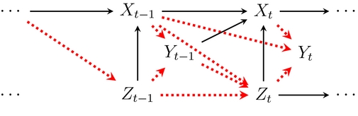
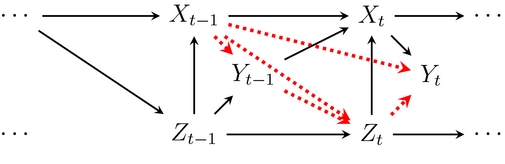
Here, the expectations are over the units so that this quantity is the average difference in outcomes between the world where all units had history x 1: t and the world where all units had history x′1: t. For example, we might be interested in the effect of a country having always high welfare spending versus a country always having low spending levels. Thus, this quantity considers the effect of treatment at time t, but also the effect of all lagged values of the treatment as well. A graphical depiction of the pathways contained in τ(x 1: t, x′1: t) is presented in Figure 1, where the dotted arrows correspond to components of the effect. These arrows represent all of the effects of X it, X i, t − 1, X i, t − 2, and so on, that end up at Y it. Note that many of these effects flow through the time-varying covariates, Z it. This point complicates the estimation of causal effects in this setting and we return to it below.
Directed acyclic graph (DAG) of typical TSCS data. Dotted lines are the causal pathways that constitute the average causal effect of a treatment history at time t.

Marginal Effects of Recent Treatments
As mentioned above, there are numerous possible treatment histories to compare when estimating causal effects. This can be daunting for applied researchers who may only be interested in the effects of the first few lags of welfare spending. Furthermore, any particular treatment history may not be well-represented in the data if the number of time periods is moderate. To avoid these problems, we introduce causal quantities that focus on recent values of treatment and average over more distant lags. We define the potential outcomes just intervening on treatment the last j periods as Y it(x t − j:t) = Y it(X i, 1:t − j − 1, x t − j:t). This “marginal” potential outcome represents the potential or counterfactual level of terrorism in country i if we let welfare spending run its natural course up to t − j − 1 and just set the last j lags of spending to x t − j:t.Footnote 3
With this definition in hand, we can define one important quantity of interest, the contemporaneous effect of treatment (CET) of X it on Y it:
 $$\begin{eqnarray*}
\tau _{c}(t) &=& E[Y_{it}(X_{i,1:\,t-1}, 1) - Y_{it}(X_{i,1:\,t-1},0)] , \nonumber \\
&=& E[Y_{it}(1) - Y_{it}(0)],
\end{eqnarray*}$$
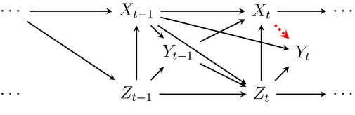
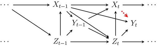
Here we have switched from potential outcomes that depend on the entire history to potential outcomes that only depend on treatment in time t. The CET reflects the effect of treatment in period t on the outcome in period t, averaging across all of the treatment histories up to period t. Thus, it would be the expected effect of switching a random country from low levels of welfare spending to high levels in period t. A graphical depiction of a CET is presented in Figure 2, where the dotted arrow corresponds to component of the effect. It is common in pooled TSCS analyses to assume that this effect is constant over time so that τc(t) = τc.
DAG of a TSCS setting where the dotted line represents the contemporaneous effect of treatment at time t.
Researchers are also often interested in how more distant changes to treatment affect the outcome. Thus, we define the lagged effect of treatment, which is the marginal effect of treatment in time t − 1 on the outcome in time t, holding treatment at time t fixed: E[Y it(1, 0) − Y it(0, 0)]. More generally, the j-step lagged effect is defined as follows:
 $$\begin{eqnarray}
\tau _{l}(t, j) &=& E[Y_{it}(X_{i,1:\,t-j-1}, 1, 0_{j}) - Y_{it}(X_{i,1:\,t-j-1}, 0,0_{j})] , \nonumber \\
&=& E[Y_{it}(1,0_{j}) - Y_{it}(0_{j+1})],
\end{eqnarray}$$
where 0s is a vector of s zero values. For example, the two-step lagged effect would be E[Y it(1, 0, 0) − Y it(0, 0, 0)] and represents the effect of welfare spending two years ago on terrorism today holding the intervening welfare spending fixed at low levels. A graphical depiction of the one-step lagged effect is presented in Figure 3, where again the dotted arrows correspond to components of the effect. These effects are similar to a common quantity of interest in both time-series and TSCS applications called the impulse response (Box, Jenkins, and Reinsel Reference Box, Jenkins and Reinsel2013).
DAG of a panel setting where the dotted lines represent the paths that constitute the lagged effect of treatment at time t − 1 on the outcome at time t.

Another common quantity of interest in the TSCS literature is the step response, which is the cumulative effect of a permanent shift in treatment status on some future outcome (Box, Jenkins, and Reinsel Reference Box, Jenkins and Reinsel2013; Beck and Katz Reference Beck and Katz2011). The step response function, or SRF, describes how this effect varies by time period and distance between the shift and the outcome:
 $$\begin{equation}
\tau _s(t,j) = E[Y_{it}(1_{j}) - Y_{it}(0_{j})],
\end{equation}$$
where 1s has a similar definition to 0s. Thus, τs(t, j) is the effect of j periods of treatment starting at time t − j on the outcome at time t. Without further assumptions, there are separate lagged effects and step responses for each pair of periods. As we discuss next, traditional modeling of TSCS data imposes restrictions on the data-generating processes, in part, to summarize this large number of effects with a few parameters.
Relationship to Traditional TSCS Models
The potential outcomes and causal effects defined above are completely nonparametric in the sense that they impose no restrictions on the distribution of Y it. To situate these quantities in the TSCS literature, it is helpful to see how they are parameterized in a particular TSCS model. One general model that encompasses many different possible specifications is an ADL model:Footnote 4
 $$\begin{equation}
Y_{it} = \beta _0 + \alpha Y_{i,t-1} + \beta _1 X_{it} + \beta _2X_{i,t-1} + \varepsilon _{it},
\end{equation}$$
where εit are independent and identically distributed errors, independent of X is for all t and s. The key features of such a model are the presence of lagged independent and dependent variables and the exogeneity of the independent variables. This model for the outcome would imply the following form for the potential outcomes:
 $$\begin{equation}
Y_{it}(x_{1:\,t}) = \beta _0 + \alpha Y_{i,t-1}(x_{1:\,t-1}) + \beta _1x_{t} + \beta _2x_{t-1} + \varepsilon _{it}.
\end{equation}$$
In this form, it is clear to see what TSCS scholars have long pointed out: causal effects are complicated with lagged dependent variables (LDVs) since a change in x t − 1 can have both a direct effect on Y it and an indirect effect through Y i, t − 1. This is why even seemingly simple TSCS models such as the ADL imply quite complicated expressions for long-run effects.
The ADL model also has implications for the various causal quantities, both short term and long term. The coefficient on the contemporaneous treatment, β1, is constant over time and does not depend on past values of the treatment, so it is equal to the CET, τc(t) = β1. One can derive the lagged effects from different combinations of α, β1, and β2:
 $$\begin{equation}
\tau _l(t,0) & = & \beta _1,
\end{equation}$$\\
 $$\begin{equation}
\tau _l(t,1) & = & \alpha \beta _1 + \beta _2,
\end{equation}$$\\
 $$\begin{equation}
\tau _l(t,2) & = & \alpha ^2\beta _1 + \alpha \beta _2.
\end{equation}$$
 $$\begin{equation}
\tau _s(t,0) & = & \beta _1,
\end{equation}$$ \\
 $$\begin{equation}
\tau _s(t,1) & = & \beta _1 + \alpha \beta _1 + \beta _2,
\end{equation}$$\\
 $$\begin{equation}
\tau _s(t,2) & = & \beta _1 + \alpha \beta _1 + \beta _2 + \alpha ^2\beta _1 + \alpha \beta _2.
\end{equation}$$
CAUSAL ASSUMPTIONS AND DESIGNS IN TSCS DATA
Under what assumptions are the above causal quantities identified? When we have repeated measurements on the outcome-treatment relationship, there are a number of assumptions we could invoke to identify causal effects. In this section, we discuss several of these assumptions. We focus on cross-sectional assumptions given our fixed time-window approach. That is, we make no assumptions on the time-series processes such as stationarity even though imposing these types of assumptions will not materially affect our conclusions about the bias of traditional TSCS methods. This result is confirmed in the simulations below, where the data generating process is stationary and the biases we describe below still occur.
Baseline Randomized Treatments
A powerful, if rare, research design for TSCS data is one that randomly assigns the entire history of treatment, X 1: T, at time t = 0. Under this assumption, treatment at time t cannot be affected by, say, previous values of the outcome or time-varying covariates. In terms of potential outcomes, the baseline randomized treatment history assumption is
 $$\begin{equation}
\lbrace Y_{it}(x_{1:\,t}): t=1,\ldots ,T\rbrace \perp \!\!\!\perp X_{i, 1:\,t} | Z_{i0},
\end{equation}$$
where A⊥⊥B|C is defined as “A is independent of B conditional on C.” This assumes that the entire history of welfare spending is independent of all potential levels of terrorism, possibly conditional on baseline (that is, time-invariant) covariates. Hernán, Brumback, and Robins (Reference Hernán, Brumback and Robins2001) called X i, 1: t causally exogenous under this assumption. The lack of time-varying covariates or past values of Y it on the right-hand side of the conditioning bar in Equation (12) implies that these variables do not confound the relationship between the treatment and the outcome. For example, this assumes there are no time-varying covariates that affect both welfare spending and the number of terrorist incidents. Thus, baseline randomization relies on strong assumptions that are rarely satisfied outside of randomized experiments and is unsuitable for most observational TSCS studies.Footnote 5
Baseline randomization is closely related to exogeneity assumptions in linear TSCS models. For example, suppose we had the following distributed lag model with no autoregressive component:
 $$\begin{equation}
Y_{it} = \beta _0 + \beta _1X_{it} + \beta _2X_{i,t-1} + \eta _{it}.
\end{equation}$$
Here, baseline randomization of the treatment history, combined with the assumptions implicit in linear TSCS models, implies the usual identifying assumption in these models, strict exogeneity of the errors:
 $$\begin{equation}
E[\eta _{it}|X_{i,1:\,T}]= E[\eta _{it}] = 0.
\end{equation}$$
This is a mean independence assumption about the relationship between the errors, ηit, and the treatment history, X i, 1: T.
Sequentially Randomized Treatments
Beginning with Robins (Reference Robins1986), scholars in epidemiology have expanded the potential outcomes framework to handle weaker identifying assumptions than baseline randomization. These innovations centered on sequentially randomized experiments, where at each period, X it was randomized conditional on the past values of the treatment and time-varying covariates (including past values of the outcome). Under this sequential ignorability assumption, the treatment is randomly assigned not at the beginning of the process, but at each point in time and can be affected by the past values of the covariates and the outcome.
At its core, sequential ignorability assumes there is some function or subset of the observed history up to time t, V it = g(X i, 1:t − 1, Y i, 1:t − 1, Z i, 1: t), that is sufficient to satisfy no unmeasured confounders for the effect of X it on future outcomes. Formally, the assumption states that, conditional on this set of variables, V it, the treatment at time t is independent of the potential outcomes at time t:
Assumption 1 (Sequential Ignorability). For every treatment history x1: T and period t,
 $$\begin{equation}
\lbrace Y_{is}(x_{1:s}): s = t,, \ldots , T\rbrace \perp \!\!\!\perp X_{it} | V_{it}.
\end{equation}$$
For example, a researcher might assume that sequential ignorability for current welfare spending holds conditional on lagged levels of terrorism, lagged welfare spending, and some contemporaneous covariates, so that V it = {Y i, t − 1, X i, t − 1, Z it}. Unlike baseline randomization and strict exogeneity, it allows for observed time-varying covariates like conflict status and lagged values of terrorism to confound the relationship between welfare spending and current terrorism levels, so long as we have measures of these confounders. Furthermore, these time-varying covariates can be affected by past values of welfare spending.
In the context of traditional linear TSCS models such as Equation (4), with their implicit assumptions, sequential ignorability implies the sequential exogeneity assumption:
 $$\begin{equation}
E[\varepsilon _{it}|X_{i,1:\,t}, Z_{i,1:\,t}, Y_{i,1:\,t-1}] = E[\varepsilon _{it}|X_{it}, V_{it}] = 0.
\end{equation}$$
According to the model in Equation (4), the time-varying covariates here would include the LDV. This assumption states that the errors of the TSCS model are mean independent of welfare spending at time t given the conditioning set that depends on the history of the data up to t. Thus, this allows the errors for levels of terrorism to be related to future values of welfare spending.
Sequential ignorability weakens baseline randomization to allow for feedback between the treatment status and the time-varying covariates, including lagged outcomes. For instance, sequential ignorability allows for the welfare spending of a country to impact future levels of terrorism and for this terrorism to affect future welfare spending. Thus, in this dynamic case, treatments can affect the covariates and so the covariates also have potential responses: Z it(x 1:t − 1). This dynamic feedback implies that the lagged treatment may have both a direct effect on the outcome and an indirect effect through these covariates. For example, welfare spending might directly affect terrorism by reducing resentment among potential terrorists, but it might also have an indirect effect if it helps to increase levels of state capacity which could, in turn, help combat future terrorism.
In TSCS models, the LDV, is often included in the above time-varying conditioning set, V it, to assess the dynamics of the time-series process or to capture the effects of longer lags of treatment in a simple manner.Footnote 6 In either case, sequential ignorability would allow the LDV to have an effect on the treatment history as well, but baseline randomization would not. For instance, welfare spending may have a strong effect on terrorism levels which, in turn, affect future welfare spending. Under this type of feedback, an LDV must be in the conditioning set V it and strict exogeneity will be violated.
Unmeasured Confounding and Fixed Effects Assumptions
Sequential ignorability is a selection-on-observables assumption—the researcher must be able to choose a (time-varying) conditioning set to eliminate any confounding. An oft-cited benefit of having repeated observations is that it allows scholars to estimate causal effects in spite of time-constant unmeasured confounders. Linear fixed effects models have the benefit of adjusting for all time-constant covariates, measured or unmeasured. This would be very helpful if, for instance, each country had its own baseline level of welfare spending that was determined by factors correlated with terrorist attacks, but the year-to-year variation in spending within a country was exogenous. At first glance, this ability to avoid time-constant omitted variable bias appears to be a huge benefit.
Unfortunately, these fixed effects estimation strategies require within-unit baseline randomization to identify any quantity other than the CET (Sobel Reference Sobel2012; Imai and Kim Reference Imai and Kim2017). Specifically, standard fixed effects models assume that previous values of covariates like GDP growth or lagged terrorist attacks (that is, the LDV) have no impact on the current value of welfare spending. Thus, to estimate any effects of lagged treatment, fixed effects models would allow for time-constant unmeasured confounding but would also rule out a large number of TSCS applications where there is feedback between the covariates and the treatment. Furthermore, the assumptions of fixed-effects-style models in nonlinear settings can impose strong restrictions on over-time variation in the treatment and outcome (Chernozhukov et al. Reference Chernozhukov, Fernndez-Val, Hahn and Newey2013). For these reasons, and because there is a large TSCS literature in political science that relies on selection-on-observables assumptions, we focus on situations where sequential ignorability holds. We return to the avenues for future research on fixed effects models in this setting in the conclusion.
THE POST-TREATMENT BIAS OF TRADITIONAL TSCS MODELS
Under sequential ignorability, standard TSCS models like the ADL model above can become biased for common TSCS estimands. The basic problem with these models is that sequential ignorability allows for the possibility of post-treatment bias when estimating lagged effects in the ADL model. While this problem is well known in statistics (Rosenbaum Reference Rosenbaum1984; Robins Reference Robins and Berkane1997; Robins, Greenland, and Hu Reference Robins, Greenland and Hu1999), we review it here in the context of TSCS models to highlight the potential for biased and inconsistent estimators.
The root of the bias in the ADL approach is the nature of time-varying covariates, Z it. Under the assumption of baseline randomization, there is no need to control or adjust for these covariates beyond the baseline covariates, Z i0, because treatment is assigned at baseline—future covariates cannot confound past treatment assignment. The ADL approach thrives in this setting. But when baseline randomization is implausible, as we argue is true in most TSCS settings, we will typically require conditioning on these covariates to obtain credible causal estimates. And this conditioning on Z it is what can create large biases in the ADL approach.
To demonstrate the potential for bias, we focus on a simple case where we are only interested in the first two lags of treatment and sequential ignorability assumption holds with V it = {Y i, t − 1, Z it, X i, t − 1}. This means that treatment is randomly assigned conditional on the contemporaneous value of the time-varying covariate and the lagged values of the outcome and the treatment. Given this setting, the ADL approach would model the outcome as follows:
 $$\begin{eqnarray}
Y_{it} = \beta _0 + \alpha Y_{i,t-1} + \beta _1 X_{it} + \beta _2X_{i,t-1} + Z_{it}^{\prime }\delta + \varepsilon _{it}. \nonumber\\
\end{eqnarray}$$
Assuming this functional form is correct and assuming that εit are independent and identically distributed, this model would consistently estimate the CET, β1, given the sequential ignorability assumption. But what about the effect of lagged treatment? In the ADL approach, one would combine the coefficients as  $\widehat{\alpha }\widehat{\beta }_1 + \widehat{\beta }_2$. The problem with this approach is that, if Z it is affected by X i, t − 1, then Z it will be post-treatment and in many cases induce bias in the estimation of
 $\widehat{\beta }_2$ (Rosenbaum Reference Rosenbaum1984; Acharya, Blackwell, and Sen Reference Acharya, Blackwell and Sen2016). Why not simply omit Z it from our model? Because this would bias the estimates of the contemporary treatment effect,
 $\widehat{\beta }_1$ due to omitted variable bias.Footnote 7
In this setting, there is no way to estimate the direct effect of lagged treatment without bias with a single ADL model. Unfortunately, even weakening the parametric modeling assumptions via matching or generalized additive models will fail to overcome this problem—it is inherent to the data generating process (Robins Reference Robins and Berkane1997). These biases exist even in favorable settings for the ADL, such as when the outcome is stationary and treatment effects are constant over time. Furthermore, as discussed above, standard fixed effects models cannot eliminate this bias because it involves time-dependent causal feedback. Traditional approaches can only avoid the bias under special circumstances such as when treatment is randomly assigned at baseline or when the time-varying covariates are completely unaffected by treatment. Both of these assumptions lack plausibility in TSCS settings, which is why many TSCS studies control for time-varying covariates. Below, we demonstrate this bias in simulations, but we first turn to two methods from biostatistics that can avoid these biases.
TWO METHODS FOR ESTIMATING THE EFFECT OF TREATMENT HISTORIES
If the traditional ADL model is biased in the presence of time-varying covariates, how can we proceed with estimating both contemporaneous and lagged effect of treatment in the TSCS setting? In this section, we show how to estimate these causal quantities of interest defined above under sequential ignorability using two approaches developed in biostatistics to specifically address this potential for bias in this type of setting. The first approach is based on SNMMs, which, in their simplest form, represent an extension of the ADL approach to avoid the post-treatment bias described above. The second class of estimators, based on MSMs and IPTW, is semiparametric in the sense that it models the treatment history, but leaves the relationship between the outcome and the time-varying covariates unspecified. Because of this, MSMs have the advantage of being robust to our ability or inability to model the outcome. We focus our attention on these two broad classes of models because they are commonly used approaches that both (a) avoid post-treatment bias in this setting and (b) do not require the parametric modeling of the distribution of the time-varying covariates.
One modeling choice that is common to all of these approaches, including the ADL, is the choice of causal lag length. Should we attempt to estimate the effect of the entire history of welfare spending on terrorist incidents with potential outcome Y it(x 1: t)? Or should we only investigate the contemporaneous and first lagged effects with potential outcome Y it(x t − 1, x t)? As we discussed above, we can always focus on effects that marginalize over lags of treatment beyond the scope of our investigation. Thus, this choice of lag length is less about the “correct” specification and more about choosing what question the researcher wants to answer. A separate question is what variables and their lags need to be included in the various models for our answers to be correct. We discuss the details of what needs to be controlled for and when in our discussion of each estimator.
Structural Nested Mean Models
Our first class of models, SNMMs, can be seen as an extension of the ADL approach that allows for estimation of lagged effects in a relatively straightforward manner (Robins Reference Robins1986, Reference Robins and Berkane1997). At their most general, these models focus on parameterizing a conditional version of the lagged effects (that is, the impulse response function):Footnote 8
 $$\begin{eqnarray}
b_t(x_{1:\,t}, j) &=& E[Y_{it}(x_{1:\,t-j},0_{j}) \nonumber\\
&&-\, Y_{it}(x_{1:\,t-j-1}, 0_{j+1})| X_{1:\,t-j} = x_{1:\,t-j}]. \nonumber\\
\end{eqnarray}$$
Robins (Reference Robins and Berkane1997) refers to these impulse responses as “blip-down functions.” This function gives the effect of a change from 0 to x t − j in terms of welfare spending on levels of terrorism at time t, conditional on the treatment history up to time t − j. Inference in SNMMs focuses on estimating the causal parameters of this function. The conditional mean of the outcome given the covariates needs to be estimated as part of this approach, but this is seen as a nuisance function rather than the object of direct interest.
Given the chosen lag length to study, a researcher must only specify the parameters of the impulse response up to that many lags. If we chose a lag length of 1, for example, then we might parameterize the impulse response function as
 $$\begin{equation}
b_t(x_{1:\,t}, j; \gamma ) = \gamma _{j}x_{t-j}, \qquad j \in \lbrace 0,1\rbrace .
\end{equation}$$
Here, γj is the impulse effect of a one-unit change of welfare spending at lag j on levels of terrorism, which does not depend on the past treatment history, x 1:t − 1 or the time period t. Keeping the desired lag length, we could generalize this specification and have an impulse response that depended on past values of the treatment:
 $$\begin{eqnarray}
b_t(x_{1:\,t}, j; \gamma ) = \gamma _{1j}x_{t-j} + \gamma _{2j}x_{t-j}x_{t-j-1}, \qquad j \in \lbrace 0,1\rbrace , \nonumber\\
\end{eqnarray}$$
where γ2j captures the interaction between contemporaneous and lagged values of welfare spending. Note that, given the definition of the impulse response, if x t-j = 0, then b t = 0 since this would be comparing the average effect of a change from 0 to 0. Choosing this function is similar to modeling X i, t − j in a regression—it requires the analyst to decide what nonlinearities or interactions are important to include for the effect of treatment. If Y it is not continuous, it is possible to choose an alternative functional form (such as one that uses a log link) that restricts the effects to the proper scale (Vansteelandt and Joffe Reference Vansteelandt and Joffe2014).
Note that the noninteractive impulse response function in Equation (19) can be seen as an alternative parameterization of the ADL (1,1) in Equation (4). When j = 0 in Equation (19) and an ADL (1,1) model holds, then the contemporaneous effect of γ0 corresponds to the β1 parameter from the ADL model. When j = 1 in Equation (19) and an ADL (1,1) model holds, then the impulse response effect of γ1 corresponds to the αβ1 + β2 combination of parameters from the ADL model. We derive this connection in more detail below, but one important difference can be seen in this example. The SNMM approach directly models the lagged effects while the ADL model recreates these effects from all constituent path effects.
The key to the SNMM identification approach is that problems of post-treatment bias can be avoided by using a transformation of the outcome that leads to easy estimation of each conditional impulse responses (γj). This transformation is
 $$\begin{equation}
\widetilde{Y}^j_{it} = Y_{it} - \sum ^{j-1}_{s=0} b_{t}(X_{i,1:\,t}, s),
\end{equation}$$
which, under the modeling assumptions of Equation (19), would be
 $$\begin{equation}
\widetilde{Y}^j_{it} = Y_{it} - \sum ^{j-1}_{s=0} \gamma _{s}X_{i,t-s}.
\end{equation}$$
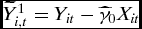
These transformed outcomes are called the blipped-down or demediated outcomes. For example, the first blipped-down outcome, which we will use to estimate first lagged effect, subtracts the contemporaneous effect for each unit off of the outcome,  $\widetilde{Y}^1_{it} = Y_{it} - \gamma _0X_{it}$. Intuitively, the blip-down transformation subtracts off the effect of j lags of treatment, creating an estimate of the counterfactual level of terrorism at time t if welfare spending had been set to zero for j periods before t. Robins (Reference Robins1994) and Robins (Reference Robins and Berkane1997) show that, under sequential ignorability, the transformed outcome,
 $\widetilde{Y}^j_{it}$, has the same expectation as this counterfactual, Y it(x 1:t − j, 0j), conditional on the past. Thus, we can use the relationship between
 $\widetilde{Y}^j_{it}$ and X i, t − j as an estimate of the j-step lagged effect of treatment, which can be used to create
 $\widetilde{Y}^{j+1}_{it}$ and estimate the lagged effect for j + 1. This recursive structure of the modeling is what gives SNMM the “nested” moniker.
We focus on one approach to estimating the parameters called sequential g-estimation in the biostatistics literature (Vansteelandt Reference Vansteelandt2009).Footnote 9 This approach is similar to an extension of the standard ADL model in the sense that it requires modeling the conditional mean of the (transformed) outcome to estimate the effect of each lag under study. In particular, for lag j the researcher must specify a linear regression of  $\widetilde{Y}^{j}_{it}$ on the variables in the assumed impulse response function, b t(x 1: t, j; γ) and whatever covariates are needed to satisfy sequential ignorability.
For example, suppose we focused on the contemporaneous effect and the first lagged effect of welfare spending and we adopted the simple impulse response b t(x 1: t, j; γ) = γjx t − j for both of these effects. As above, we assume that sequential ignorability held conditional on V it = {X i, t − 1, Y i, t − 1, Z it}. Sequential g-estimation involves the following steps:
1. For j = 0, we would regress the untransformed outcome on {X it, X i, t − 1, Y i, t − 1, Z it}, just as we would for the ADL model. If the modeling is correctly specified (as we would assume with the ADL approach), the coefficient on X it in this regression will provide an estimate of the blip-down parameter, γ0 (the contemporaneous effect).
2. We would use
 $\widehat{\gamma }_0$ to construct the one-lag blipped-down outcome, $\widetilde{Y}^1_{i,t} = Y_{it} - \widehat{\gamma }_0X_{it}$.
3. This blipped-down outcome would be regressed on {X i, t − 1, X i, t − 2, Y i, t − 2, Z i, t − 1} to estimate the next blip-down parameter, γ1 (the first lagged effect).

If more than two lags are desired, we could use  $\widehat{\gamma }_1$ to construct the second set of blipped-down outcomes,
 $\widetilde{Y}^2_{i,t} = \widetilde{Y}^1_{i,t} - \widehat{\gamma }_1X_{i,t-1}$, which could then be regressed on {X i, t − 2, X i, t − 3, Y i, t − 3, Z i, t − 2} to estimate γ2. This iteration can continue for as many lags as desired. This approach avoids including a post-treatment covariate when estimating a particular lagged effect. That is, when estimating the effect of welfare spending at lag j, only variables causally prior to welfare spending at that point are included in the regression. Standard errors for all of the estimated effects can be estimated using a consistent variance estimator presented in the Supplemental Material or via a block bootstrap.
This sequential g-estimation approach requires the correct specification of the relationship between the (transformed) outcome and the covariate and treatment histories. It thus requires a similar regression model to the ADL approach described above. More complicated SNMM estimators can incorporate a model for the treatment process, providing some robustness to the modeling choices for the outcome. These estimators are consistent for the parameters of the SNMM when either the model for the (transformed) outcome or the model for the treatment process is correctly specified. This property is called double robustness because there are “two shots” to achieve consistency. Vansteelandt and Joffe (Reference Vansteelandt and Joffe2014) provides a review of these methods for SNMMs.
Relationship to the ADL model
As we mentioned above, the ADL approach and the sequential g-estimation version of SNMM presented above are very similar when the time-varying covariates, Z it, are not affected by treatment. One intuition for this result is that the ADL model and the SNMM with the linear model are equivalent when there are no covariates aside from the LDV. To see this, suppose that the ADL model in Equation (4) is correct and perform the first transformation from step 2 above, noting, as above, that the contemporaneous effect is the same for both models γ0 = β1:
 $$\begin{equation}
Y_{it} - \gamma _0X_{it} = Y_{it} - \beta _1X_{it}
\end{equation}$$
 $$\begin{equation}
= \beta _0 + \alpha Y_{i,t-1} + \beta _2X_{i,t-1} + \varepsilon _{it}
\end{equation}$$
 $$\begin{eqnarray}
&=& \beta _0 + \alpha (\beta _0 + \alpha Y_{i,t-2} + \beta _1X_{i,t-1} + \beta _2X_{i,t-2} \nonumber\\
&&+\, \varepsilon _{i,t-1}) + \beta _2X_{i,t-1} + \varepsilon _{it}
\end{eqnarray}$$
 $$\begin{eqnarray}
&=& (\beta _0 + \alpha \beta _0) + \alpha ^2 Y_{i,t-2} + \underbrace{(\alpha \beta _1 + \beta _2)}_{\gamma _1}X_{i,t-1} \nonumber\\
&&+\, \alpha \beta _2X_{i,t-2} + (\alpha \varepsilon _{i,t-1} + \varepsilon _{it}).
\end{eqnarray}$$
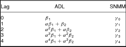
From this, we can see that the coefficient on X i, t − 1 for this transformed outcome is simply the impulse response at lag 1, which is exactly the quantity that the SNMM targets. Given the ADL and SNMM assumptions above, this quantity will be αβ1 + β2 for the ADL model and γ1 for the SNMM. Of course, this correspondence will continue for all lagged effects and Table 1 shows how the two sets of quantities relate for various lags.
The lagged effects, or impulse responses, under the ADL (1,1) in Equation (4) and SNMM in Equation (19).

Furthermore, in the Supplemental Material, we show that the sequential g-estimation estimator with no covariates except an LDV is nearly mechanically equivalent to a traditional ADL estimator with one lag. The difference is that the traditional ADL model relies on an assumption that the contemporaneous effect is constant over time, whereas sequential g-estimation relaxes this assumption. This provides a useful interpretation of the ADL model in terms of counterfactual causal effects. It is important to note, however, that this equivalence also relies on the form of the ADL model, which uses only three parameters regardless of the number of lags, while the SNMM in this version uses a new parameter for every lag. Additionally, the near equivalence disappears once there is an additional time-varying covariate (Z it) in the model.
Marginal Structural Models
One potential downside of the SNMM approach is that it requires the analyst to correctly model the relationship between the time-varying covariates and the outcome. This can be difficult when the outcome is a complicated process and there is little theoretical guidance for specifying the outcome-covariate relationships. An alternative that relies instead on modeling the treatment-covariate relationship is called a marginal structural model or MSM (Robins, Hernán, and Brumback Reference Robins, Hernán and Brumback2000).Footnote 10 To specify an MSM, we first choose a potential outcome lag length to study and write a model for the marginal mean of those potential outcomes in terms of the treatment history. At the most general, then, an MSM would be the following:
 $$\begin{equation}
E[Y_{it}(x_{1:\,t})] = g(x_{1:\,t};\beta ),
\end{equation}$$
where the function g operates similarly to a link function in a generalized linear model.Footnote 11 These models are similar to the impulse response functions in the SNMM approach, b t, because they provide structure for the treatment-outcome relationship. For instance, suppose that we were focused on the contemporaneous effect and the effect of the first two lags and so we had to model E[Y it(x t − 2:t)] = g(x t − 2:t; β), marginalizing over further lags and other covariates. If Y it were approximately continuous, as in the case of the number of terrorist incidents, we might take g to be linear and focus on the additive effects of each period of treatment:Footnote 12
 $$\begin{equation}
g(x_{t-2:t};\beta ) = \beta _0 + \beta _1x_{t} + \beta _2x_{t-1} + \beta _3x_{t-2}.\vspace*{-2pt}
\end{equation}$$
If Y it were binary, we might instead assume g to have a logistic form:
 $$\begin{eqnarray}
g(x_{t-2:t};\beta ) = \frac{\exp (\beta _0 + \beta _1x_{t} + \beta _2x_{t-1} + \beta _3x_{t-2})}{1 + \exp (\beta _0 + \beta _1x_{t} + \beta _2x_{t-1} + \beta _3x_{t-2})}. \nonumber\\\vspace*{-2pt}
\end{eqnarray}$$
In both of these cases, we have restricted our attention to the last three periods of treatment and so we cannot answer questions about longer-term effects with these models. On the other hand, as we increase the number of lags under study, the number of parameters needed to summarize the effects grows and the model can become unwieldy. Thus, we may consider focusing on the effect of the cumulative number of treated periods, ∑ts = 1xis. This allows for the entire history of treatment to affect the outcome in a structured, low-dimensional way. Under any of these models, the average causal effect becomes
 $$\begin{equation}
\tau (x_{1:\,t},x^{\prime }_{1:\,t}) = g(x_{1:\,t};\beta ) - g(x_{1:\,t}^{\prime };\beta ). \vspace*{-2pt}
\end{equation}$$
Of course, the MSM specification will place restrictions on the average causal effects. An MSM that is a function of only the cumulative treatment, for instance, implies that τ(x 1: t, x′1: t) = 0 if x 1: t and x′1: t have the same number of treated periods, even if their sequence differs.
How can a researcher estimate an MSM? If one blindly follows model Equation (28) and regresses Y it on {X i, t − 2, X i, t − 1, X it} using ordinary least squares, there will be omitted variable bias in the estimated coefficients. But as we have seen above, simply including time-varying covariates in these models can lead to post-treatment bias. Fortunately, the causal parameters of these models are estimable using an IPTW approach where we adjust for time-varying covariates using the propensity score weights, not the outcome model itself, avoiding post-treatment bias (Robins, Hernán, and Brumback Reference Robins, Hernán and Brumback2000). The weighting balances the distribution of the time-varying covariates across values of the treatments, so that omitting these variables in the reweighted data produces no omitted variable bias.
To use IPTW, a researcher must develop a model for the probability of treatment in period t given the variables that satisfy sequential ignorability. For example, suppose that sequential ignorability holds conditional on some conditioning set V it. If X it is binary, then we must obtain a consistent estimate of  $\Pr [X_{it} = 1 \;|\; V_{it} = v]$. This might be a pooled logit, a generalized additive model with a flexible functional form, a boosted regression (McCaffrey, Ridgeway, and Morral Reference McCaffrey, Ridgeway and Morral2004), or a covariate-balancing propensity score (CBPS) model (Imai and Ratkovic Reference Imai and Ratkovic2015). The IPTW approach requires this model to provide consistent estimates of the conditional predicted probability of treatment.Footnote 13 In spite of this requirement, some methods for propensity score estimation such as CBPS have good finite-sample properties in the face of model misspecification (Imai and Ratkovic Reference Imai and Ratkovic2015).
We use the predicted probabilities from this treatment model to construct weights for each country-year. For example, suppose that V it included lagged levels of terrorism, Y i, t − 1, lagged welfare spending, X i, t − 1, and a set of time-varying covariates, Z it. Then, for a binary treatment, we would construct the weights as
 $$\begin{equation}
\widehat{SW}_{it} = \prod _{t = 1}^t \frac{\widehat{\Pr }[X_{it} \;|\; X_{i,t-1}; \widehat{\gamma }]}{\widehat{\Pr }[X_{it} \;|\; Z_{it}, Y_{i,t-1}, X_{i,t-1}; \widehat{\alpha }]}.
\end{equation}$$
The denominator of each term in the product is the predicted probability of observing unit i’s observed treatment status in time t (X it), conditional on the covariates that satisfy sequential ignorability.Footnote 14 When we multiply this over time, it is the probability of seeing this unit’s treatment history conditional on the past. The numerators here are the marginal probability of the observed treatment history and stabilize the weights to make sure they are not too variable which can lead to poor finite sample performance (Cole and Hernán Reference Cole and Hernán2008). For instance, to construct this numerator we might run a pooled logistic regression of welfare spending in year t on welfare spending in year t − 1, omitting any time-varying covariates or LDVs. While this choice of numerator is not required for consistency of the estimator (it can be replaced with 1, for instance), it can help to stabilize weights that are highly variable and thus increase efficiency.
Under these assumptions, the expectation of Y it conditional on X i, 1: t in the reweighted data converges to the true MSM:
 $$\begin{equation}
E_{\widehat{SW}}[Y_{it}|X_{i,1:\,t} = x_{1:\,t}] \stackrel{p}{\rightarrow } E[Y_{it}(x_{1:\,t})].
\end{equation}$$
Here  $E_{\widehat{SW}}[\cdot ]$ is the expectation in the reweighted data. For example, if we used the linear MSM in Equation (28), then we can estimate the causal parameters of MSM by running a weighted least squares (WLS) regression of the outcome, Y it on {X i, t − 2, X i, t − 1, X it} with
 $\widehat{SW}_{it}$ as the weights. If sequential ignorability holds, the coefficients on the components of X i, 1: t from this regression will have a causal interpretation, though they may depend on the particular modeling choices of the MSM (Robins, Hernán, and Brumback Reference Robins, Hernán and Brumback2000). Standard errors can be estimated via a block bootstrap of units. Note that, unlike the ADL and SNMMs, this approach does not require a model for the relationship between the time-varying covariates and the outcome.
Finally, when the conditional probability of treatment is close to zero or one, the IPTW approach can have large and unstable weights, leading to high variance and sometimes small sample biases (Imai and Ratkovic Reference Imai and Ratkovic2015). SNMMs, on the other hand, tend to be more stable in this setting. And while MSMs and SNMMs can accommodate general types of covariates, SNMMs also tend to be more stable when the treatment is continuous since weighting by a continuous density (as would be required with IPTW) is sensitive to small perturbations in the data (Goetgeluk, Vansteelandt, and Goetghebeur Reference Goetgeluk, Vansteelandt and Goetghebeur2008).
Modeling Checklist
In this section, we review the key modeling choices required to implement these methods.
Causal lag length
First, one must choose the lag length to study. At the most general, one can investigate the effect of an entire treatment history, but these are usually too highly dimensional to study without further assumptions. In MSMs, one can reduce this dimensionality by assuming that treatment history only affects the outcome through the average level of treatment or the cumulative amount of treatment up to time t. Alternatively, a researcher can focus on the marginal effects of the last j lags of treatment.
Conditioning set for sequential ignorability
Separate from the question of what to study is the question of what covariates to choose so that the question can be answered. Sequential ignorability is an assumption about conditional independence: welfare spending is independent of the potential outcomes conditional on past treatment and some set of baseline and time-varying covariates. Thus, scholars must choose a set of covariates for each time period that blocks all confounding for the treatment-outcome relationship—that is, there must be no omitted variables after controlling for that conditioning set. In the context of welfare spending, these covariates might include lagged welfare spending (X i, t − 1) and the lagged terrorist activity (Y i, t − 1), time-varying economic factors like GDP growth unemployment (Z it), and baseline characteristics such as region of the world (Z i0). This conditioning set of variables will be included in the models for the outcome in the SNMM approach or in the models for the treatment in the MSM approach.
Modeling treatment or outcome
In all of the methods described in this paper, the analyst must specify the functional form of how the treatment history and outcome relate. In the SNMM approach, this is done through the blip-down functions while, in the MSM, this is done through the specification of the MSM itself. To actually estimate these models, however, a researcher must additionally model either the relationship between the outcome and the covariates in the conditioning set (in the ADL or SNMM approaches) or the relationship between the treatment and the covariates in the conditioning set (in the MSM approach). Because the quality of the causal estimates depends on this modeling, we encourage researchers to choose the approach for which more substantive knowledge can be mustered to help with the modeling task. For example, suppose we were estimating the effect of central bank interest rate changes on support for incumbent candidates. It may be easier to model the central bank interest rate changes if we have detailed information on central bank deliberations about changes that help us specify the model. In other cases, there may be more substantive information about the outcome model.
Functional form assumptions
Finally, in either model that is chosen, the analyst must correctly specify the model in the sense that the functional form assumed for the variables in the conditioning set is correct. This may require, for instance, taking the natural log of population, including a squared term for GDP growth to allow for a nonlinear relationship, or including an interaction between two important covariates. This task is common to all modeling strategies and is not unique to the current setting. A researcher can weaken these modeling assumptions by replacing linear or generalized linear models with generalized additive models that allow the functional forms of chosen covariates to be estimated along with the other model parameters (Beck and Jackman Reference Beck and Jackman1998).Footnote 15
SIMULATION EVIDENCE
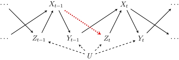
To investigate the small sample properties of the various estimators, we conducted a simulation study of a TSCS setting with a treatment, an outcome, and a single covariate, all time-varying. We describe the simulation in more detail in the Supplemental Material, but the main causal relationships in the design are displayed in Figure 4. Here, the treatment history only has a contemporaneous effects—lagged treatments, X i, 1:t − 1, and outcomes, Y i, 1:t − 1, have no direct or indirect effect on current outcomes, Y it, that don’t go through current treatment, X it. The treatment-outcome relationship is confounded due to a time-constant unmeasured confounder, U i, but conditioning on {Y i, t − 1, Z it} can block this confounding and ensure sequential ignorability for X it. Finally, the distribution of {Y it, X it, Z it} is Markovian and stationary within each unit, which should be an ideal setting for the ADL approach.
Direct acyclic graph of the simulation study. Dotted thick line represents the key causal quantity varied in the simulations, whether past treatment affects future covariates. Dashed thin lines represent unmeasured confounding.

To show how the causal structure can affect the performance of the estimators, we consider two scenarios that vary the feedback between the treatment and the time-varying covariate. In the first, we allow for lagged treatment to affect future covariates so that X i, t − 1 → Z it, and, in the second, we close this path. These two scenarios represent when the time-varying confounder, Z it, is post-treatment to lagged treatment and when it is not. Unfortunately, when Z it is post-treatment, conditioning on it will induce post-treatment bias for the effect of lagged treatment, because conditioning will open a back-door path from Z it through U i to Y it. However, we must condition on Z it to remove the omitted variable bias for contemporaneous treatment. This is the dilemma that traditional TSCS models like the ADL model cannot solve, because a single model cannot simultaneously control for Z it and not control for Z it.
We generate data from this model varying numbers of time periods and units and focus on the lagged effect of treatment, E[Y it(1, 0) − Y it(0, 0)], which in this case is zero. We compared several methods for estimating this quantity: (1) an ADL as above with estimate  $\widehat{\alpha }\widehat{\beta }_1 + \widehat{\beta }_2$; (2) an SNMM sequential g-estimation with additive linear models for the outcome for each lag; (3) a linear, additive MSM with g(x t − 1, x t; β) = β0 + β1x t + β2x t − 1; and (4) a raw model with no controls that only includes X it and X i, t − 1.Footnote 16 For reference, we also compare these estimators to the infeasible estimator that simply takes the sample average of Y it(0, 1) − Y it(0, 0) across all unit-periods.
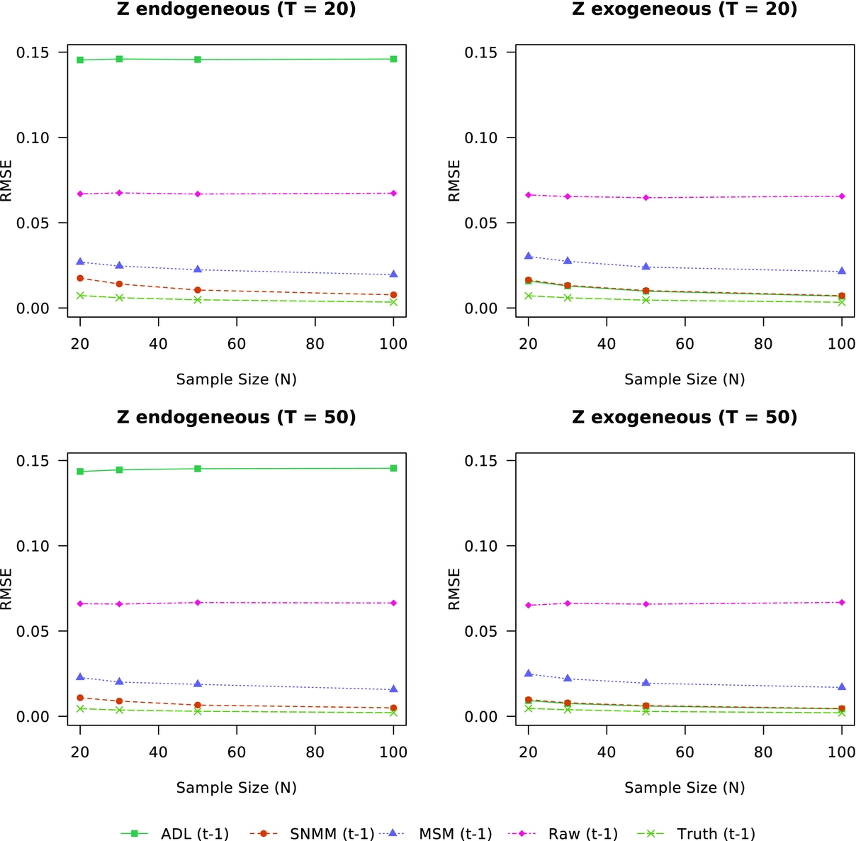
Figure 5 shows the results of these simulations. The left column shows the root mean squared error (RMSE) of the various estimators when the time-varying confounder, Z it, is affected by past treatment. While the SNMM and MSM approaches have roughly similar estimation error across different sample sizes, they vastly outperform the ADL approach. The high RMSE of the ADL approach that persists across sample sizes is due to a large degree of post-treatment bias on the coefficient on X i, t − 1 due to conditioning on Z it. This bias propagates to the ADL computation of the total effect of lagged treatment. The ADL model even performs worse than a model that has significant omitted variable bias due to excluding all time-varying covariates from the model (labelled Raw in the figure). These results hold even though the DGP here is stationary and the sample size and the number of time periods are small and similar in size, meaning that they are unlikely to depend on a “large-N, small-T” setting. Furthermore, in the Supplemental Material, we show that the same substantive results hold when we fix the value of N and let T increase to as high as 500.
Simulation results when the time-varying confounder is post-treatment (left column) and when the time-varying confounder is not post-treatment (right column). Points represent the root mean squared error (RMSE) of each estimator for the lagged effect of treatment.

The right column of Figure 5 shows the results when the time-varying confounder is not affected by treatment. Here, the ADL has lower estimation error than any of the other methods, slightly beating out SNMM. The ADL model performs well in this setting since the LDV is the only variable affected by past treatment. As we show in the Supplemental Material, in this case the ADL model is essentially a correctly specified SNMM. This correct specification breaks down when time-varying covariates are affected by treatment. Given the robustness of SNMM to this feature of the causal process and given the similarity in modeling choices for the SNMM and ADL approaches, we recommend using the SNMM as a working replacement for the ADL model whenever lagged effects are of interest.Footnote 17
EMPIRICAL ILLUSTRATION: WELFARE SPENDING AND TERRORISM
Burgoon (Reference Burgoon2006) studied the effect of domestic welfare spending on terrorist activity within countries and used TSCS data to show that increasing spending leads to lower levels of terrorist activity within a country. But how does the timing of this spending matter? Can we assess the effects of lagged government spending on future values of terrorist activity? We apply the models of this paper to show how they differ from traditional approaches to answering these questions.
To do this, we closely follow the specification of Burgoon (Reference Burgoon2006). The dependent variable is the number of transnational terrorist incidents occurring in a country, omitting purely domestic terrorism such as the Oklahoma City bombing in the United States. Burgoon (Reference Burgoon2006) uses a negative binomial regression model to estimate the effect of contemporaneous spending, whereas we use a linear model. To account for overdispersion, we use the square root of the number of transnational terrorist incidents as our dependent variable. This approach recovers very similar substantive results as that of Burgoon (Reference Burgoon2006).
A first step for any of the methods we describe in the paper is to choose a conditioning set of covariates that can satisfy sequential ignorability. Given that Burgoon (Reference Burgoon2006) interprets the effect of spending in a causal fashion, we follow this selection-on-observables approach and assume that the control variables in the paper’s models are sufficient to satisfy sequential ignorability. These include a set of regional and year dummies as baseline covariates and the following time-varying covariates: an LDV, left-party control of government, Polity score and its lag, log population, a measure of government capability, whether the country is in a conflict, and the amount of trade logged. In this context, the sequential ignorability assumption states that welfare spending is exogenous with respect to terrorism conditional on previous terrorist incidents, the time-varying covariates, and region and year fixed effects. Note that if there were unmeasured confounding beyond these controls, the estimates of causal effects in this application could be biased. One could, however, perform a sensitivity analysis to determine how much of the estimated effect disappears under various departures from sequential ignorability (Blackwell Reference Blackwell2014).
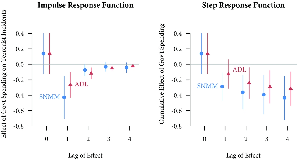
To begin, we compare how the ADL and the SNMM approaches differ in terms of their estimates in this context. For the SNMM, we assume each lag has a simple additive effect as in Equation (19), γjx t − j, with no interactions between treatment and lagged treatment. For the ADL model, we use the specification described above while including a lag of treatment in the model to allow for some flexibility in the lag structure. We use the formulas for calculating lagged effects from an ADL model, as described above. This ADL regression is also the first-stage regression for our sequential g-estimation approach, since under sequential ignorability, it can estimate the CET. We focus on a lag length of four years for comparing the SNMM and ADL approaches. Finally, we use the consistent and cluster-robust variance estimator in the Supplemental Material for the SNMM and a standard cluster-robust variance estimator for the ADL, with both clustered on country.
Figure 6 shows the estimated contemporaneous and lagged effect of welfare spending on terrorist activity. For instance, a one-year lag has  $\widehat{\gamma }_1$ for the SNMM, estimated from a regression of the blipped-down outcome on lagged treatment and its conditioning set, and
 $\widehat{\alpha }\widehat{\beta }_1 + \widehat{\beta }_2$ for the ADL approach. The two approaches are equivalent for the contemporaneous effect but differ in their estimates of the lagged effects. Both methods show a significant and negative effect on lagged spending, but the coefficient from the SNMM approach is about 60% larger in magnitude than the ADL approach. These differences continue with the lags—the effect of the second and third lags are 60% greater in the ADL approach, whereas the effect of the fourth lag is almost double the magnitude for SNMMs. These differences lead to large differences in the estimated cumulative effect of the SRF at the end of four years, with the SNMM estimate almost 40% larger in magnitude.
Left: Estimated effect of government spending on the terrorist incidents at various lags, along with 95% confidence intervals. Right: Implied step response function at various lags. Data from Burgoon (Reference Burgoon2006).

Why do these differences between the SNMM and the ADL occur? Differences in assumptions about functional forms of the covariates are ruled out since the SNMM and ADL models handle these covariates in the exact same way. Furthermore, each of the two approaches rely on a similar assumption about no unmeasured confounding. We believe that the difference between these two approaches is in the post-treatment bias induced by conditioning on the time-varying controls in the ADL approach. In this case, it is highly unlikely that the time-varying covariates are exogenous to welfare spending. For example, one time-varying covariate is the proportion of the government held by left-wing parties. It would be unreasonable to assume that past values of welfare spending are unrelated to future electoral prospects of leftist parties, as would have to be the case for the ADL model to be correct in this case. Indeed, if we regress proportion of the government controlled by leftist parties on lagged welfare spending and the conditioning set for lagged spending, there is a statistically significant and positive coefficient on lagged welfare spending. Thus, it does appear that post-treatment bias could loom large in the estimated effects of the ADL approach.
In the above analysis, we focused on a lag length of four, even though the data run from 1978 until 1995. Can we learn more about the effects of the history of welfare spending on terrorism? To do this, we turn to MSMs, where we can develop models that summarize the effects of the entire treatment history in low dimensions. We have seen that lagged welfare spending appears to have an effect, and so we may want to know if having a long history of spending also decreases incidences of terrorism. To implement this, we first create a binary measure of welfare spending, X*it, that is one if the country-year had spending (as a function of its GDP) above the global average and zero if the spending was below the average. We then specify the following MSM:
 $$\begin{equation}
E[Y_{it}(x^*_{i,1:\,t})] = \beta _0 + \beta _1 x^*_{it} + \beta _2 \left( \sum _{s=1}^{t-1} x^*_{is} \right).
\end{equation}$$
Here, the mean of the potential outcomes is a function of the contemporaneous level of spending and the number of lagged periods that have above-average spending. We focus on this simple model, though it is possible to include further lags or interactions between different parts of the history.
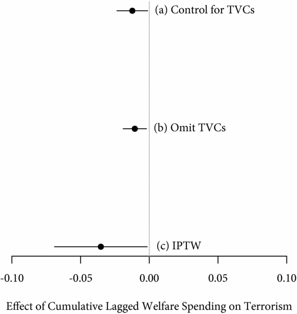
We use three approaches to estimate the parameters of the MSM. First, we take the standard ADL-like approach of including the entire set of baseline and time-varying covariates in a regression model. Second, we run the same regression with only the baseline covariates. As we have discussed above, the first of these approaches is likely to produce post-treatment bias and the second is likely to produce omitted variable bias. We compare these to a third approach that uses the IPTW method described above. To create the weights, we fit a logistic regression of the binary treatment on the first two lags of treatment, the cumulative sum of treatment through t − 3, and the baseline and time-varying covariates described above. We use predicted probabilities from this model to create the weights as in Equation (31), which we use in WLS regression of the above MSM. We use a block bootstrap to estimate standard errors and trim the weights at ten to help guard against highly unstable weights (Cole and Hernán Reference Cole and Hernán2008).
Figure 7 shows the results of these models. Both of the traditional approaches estimate a relatively small negative effect of lagged welfare spending on terrorism. The IPTW approach, on the other hand, shows a much larger negative and statistically significant impact, which is consistent with the results of the analysis from both the SNMM and ADL models above. It is interesting to note that the implied post-treatment and omitted variable biases in the first and second models, respectively, are in the same direction. This agreement tempts us to confirm the approximate validity of their results; after all, a natural intuition would be that the true effect must be between these two estimates. Unfortunately, this intuition, while natural, is incorrect. The biases of both approaches can be in the same direction, negating their usefulness as bounds (Blackwell Reference Blackwell2013). Finally, we note that the rather large increase of the standard errors in the IPTW approach is driven in part by large weights due to predicted probabilities being close to zero or one. This can happen with slowly changing treatments and is one reason to prefer an SNMM approach in this setting.
Estimated effect of the cumulative number of high welfare spending years through t − 1 on terrorism incidents in year t, fixing welfare spending in year t. The three approaches are (a) when controlling for time-varying covariates, (b) when omitting those variables, and (c) using IPTW. Lines are 95% confidence intervals based on a block bootstrap with 1,000 replications.

CONCLUSIONS, DRAWBACKS, AND FUTURE RESEARCH
Repeated measurements over time of countries, people, or governments expand the scope of causal inference methods. TSCS data allow us to estimate both contemporaneous effects and the effects of more distant lags of treatment. But with an expanded scope comes complications. The usual TSCS regression methods break down for lagged effects. Nevertheless, we have shown that two approaches developed in biostatistics can overcome these difficulties and recover effect estimates across a wide variety of settings.
Both SNMMs and MSMs have their own drawbacks, of course. Even though sequential ignorability nonparametrically identifies any average causal effect of a treatment history, both approaches will almost always depend on modeling to estimate these effects since the covariates needed to justify such an assumption will be highly dimensional. While these modeling assumptions can be weakened to some extent through generalized additive models or other semiparametric techniques, there will always be some degree of model dependence that follows from these approaches. Another problem is that sequential ignorability is a strong, untestable assumption that might be violated. One approach to mitigating this problem is to conduct a formal sensitivity analysis using the methods of Blackwell (Reference Blackwell2014) or relying on the bias formulas presented in Acharya, Blackwell, and Sen (Reference Acharya, Blackwell and Sen2016). These sensitivity analyses can give researchers a sense of how reliant their results are on sequential ignorability holding. Finally, it is important to note that the empirical setting may determine which of these two approaches is a better fit, as SNMMs are more suited to modeling the outcome and MSMs are more suited to modeling the treatment process.
In this paper, we focused on the usual sequential ignorability assumption as commonly invoked in epidemiology. Many TSCS applications in political science rely on a “fixed effects” assumption that there is time-constant, unmeasured heterogeneity in units. Linear models can easily handle these types of assumptions, though nonlinear fixed effects models pose greater difficulties. Estimating the above causal quantities with these models, however, remains elusive except under strong assumptions like baseline randomization (Chernozhukov et al. Reference Chernozhukov, Fernndez-Val, Hahn and Newey2013; Sobel Reference Sobel2012). A valuable direction for future work would be to develop fixed effects methods that could estimate causal effects under a within-unit version of sequential ignorability.
SUPPLEMENTARY MATERIAL
Replication materials can be found on Dataverse at: https://doi.org/10.7910/DVN/SFBX6Z.




Comments
No Comments have been published for this article.