1 Introduction
Liquid jets are of great significance in many industrial and medical applications as they deliver liquid matter with high velocity (Tagawa et al. Reference Tagawa, Oudalov, Visser, Peters, van der Meer, Sun, Prosperetti and Lohse2012; Gonzalez-Avila, Song & Ohl Reference Gonzalez-Avila, Song and Ohl2015) from which fine droplets develop through inherent instabilities (Eggers Reference Eggers1997; Villermaux Reference Villermaux2007; Eggers & Villermaux Reference Eggers and Villermaux2008). Jetting is frequently found in liquid phenomena involving surface singularities such as bursting of bubbles (Boulton-Stone & Blake Reference Boulton-Stone and Blake1993; Duchemin et al. Reference Duchemin, Popinet, Josserand and Zaleski2002), collapsing of bubbles near a free surface (Chahine Reference Chahine1977; Blake & Gibson Reference Blake and Gibson1981), impact of droplets or solid objects onto a deep liquid pool (Bergmann et al. Reference Bergmann, Van Der Meer, Gekle, Van Der Bos and Lohse2009; Agbaglah et al. Reference Agbaglah, Thoraval, Thoroddsen, Zhang, Fezzaa and Deegan2015), focusing pressure pulses on curve surfaces (Antkowiak et al. Reference Antkowiak, Bremond, Le Dizès and Villermaux2007; Kiyama et al. Reference Kiyama, Tagawa, Ando and Kameda2016), nonlinear Faraday waves (Longuet-Higgins Reference Longuet-Higgins1983; Zeff et al. Reference Zeff, Kleber, Fineberg and Lathrop2000), focusing laser pulses inside a partially liquid filled capillary tube (Tagawa et al. Reference Tagawa, Oudalov, Visser, Peters, van der Meer, Sun, Prosperetti and Lohse2012; Peters et al. Reference Peters, Tagawa, Oudalov, Sun, Prosperetti, Lohse and van der Meer2013) and focusing a laser pulse inside liquid marbles (Marston & Thoroddsen Reference Marston and Thoroddsen2015) to name a few. Recently another occurrence of jetting from single droplets has been reported by Gonzalez-Avila & Ohl (Reference Gonzalez-Avila and Ohl2016). These were induced from an explosively expanding spherical liquid surface driven by a cavitation bubble at its centre.
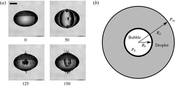
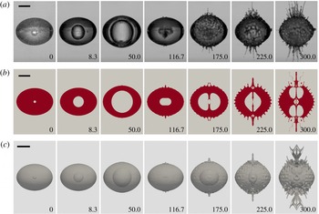
(a) An example of the jetting of a single water droplet under an internal cavitation bubble oscillation; (b) sketch of the problem. Time in
 $\unicode[STIX]{x03BC}\text{s}$
; the scale bar represents 1 mm.

A typical sequence of such jetting is illustrated in figure 1(a): a cavitation bubble generated with a focused laser pulse oscillates inside a millimetre-sized water droplet. We have selected four frames during the course of jetting depicting the stages of bubble nucleation (
 $t=0~\unicode[STIX]{x03BC}\text{s}$
), bubble expansion (
 $t=50~\unicode[STIX]{x03BC}\text{s}$
), bubble collapse (
 $t=125~\unicode[STIX]{x03BC}\text{s}$
) and its re-expansion (
 $t=150~\unicode[STIX]{x03BC}\text{s}$
). Due to the rapidly expanding bubble, the outer air–water interface is destabilized with ripples forming at the upper and lower pole of the droplet: see figure 1(a),
 $t=50~\unicode[STIX]{x03BC}\text{s}$
. During bubble shrinkage these ripples increase in size and are the sources of the fast jets observed during the re-expansion of the bubble. These jets then pinch off into fine daughter droplets. The origin of the jets is related to a Rayleigh–Taylor unstable air–water interface caused by the spherical geometry undergoing rapid radial acceleration (Gonzalez-Avila & Ohl Reference Gonzalez-Avila and Ohl2016).
The geometry of the problem is sketched in figure 1(b). After the laser has nucleated a vapour bubble we assume that at time
 $t=0$
we have a bubble with an initial radius
 $R_{b}(t=0)$
at uniform high pressure
 $P_{0}$
. The bubble is located at the centre of the droplet,
 $r=0$
, and we assume for simplicity a spherical droplet with an initial radius of
 $R_{d}(t=0)=[R_{d0}^{3}+R_{b}^{3}(t=0)]^{1/3}$
surrounded with gas, where
 $R_{d0}$
is the droplet radius before the bubble is nucleated. Far from the droplet the pressure is
 $P_{\infty }$
. The bubble oscillation within the droplet leads to a time-dependent radial acceleration. Both interfaces, the inner interface between the bubble and the droplet and the outer interface between the droplet and the surrounding gas are susceptible to Rayleigh–Taylor instabilities (Taylor Reference Taylor1950). In this work we focus on the outer interface; here the density decreases with increasing
 $r$
. The stability of the interface is quantified from the growth dynamics of the disturbances. For this we take into account the spherical geometry, the time dependence of the acceleration, surface tension and viscosity. Viscosity (Kull Reference Kull1991; Elgowainy & Ashgriz Reference Elgowainy and Ashgriz1997) and surface tension (Plesset Reference Plesset1954; Daly Reference Daly1969) in general stabilize the interface.
The spherical Rayleigh–Taylor instability is also known as the Bell–Plesset instability, for the pioneering work of Bell (Reference Bell1951) and fundamental research of Plesset (Reference Plesset1954). Bell (Reference Bell1951) was the first to consider the Rayleigh–Taylor instability in the spherical and cylindrical geometries. Later Binnie (Reference Binnie1953) proposed a solution on the spherical Rayleigh–Taylor problem for the stability analysis of a cavitation bubble surface by extending the exponential growth rate calculation of Taylor (Reference Taylor1950) from a planar surface to a spherical surface. Plesset (Reference Plesset1954) later improved the model and formulated an ordinary differential equation (ODE) for small perturbations. The ODE allows for the calculation of the stability criteria of any spherical surface separated by two incompressible, immiscible and inviscid fluids with time-dependent radial acceleration. Prosperetti (Reference Prosperetti1977) extended the formulation by accounting for viscous effects through vorticity induced by viscous stresses in the boundary layer. Prosperetti’s method has been widely applied to understand the shape stability of sonoluminescencing bubbles (Brenner, Lohse & Dupont Reference Brenner, Lohse and Dupont1995; Hilgenfeldt, Lohse & Brenner Reference Hilgenfeldt, Lohse and Brenner1996; Brenner, Hilgenfeldt & Lohse Reference Brenner, Hilgenfeldt and Lohse2002). Here, we extend the solution of Prosperetti (Reference Prosperetti1977) to our problem to analyse the stability of the droplet surface, and to couple the volume oscillation of the droplet, which is controlled by the internal bubble dynamics.
The present work is focused on the mechanism leading to jetting from droplets undergoing volume oscillation. We particularly account for the stabilizing effect of viscosity. The study encompassed experiments, computational fluid dynamics (CFD) simulations in axisymmetry and three dimensions and an analytic model for surface stability. The methodologies for all three approaches are described in § 2, results and discussions are given in § 3 and the work is summarized in § 4.
2 Methodology
2.1 Experiment
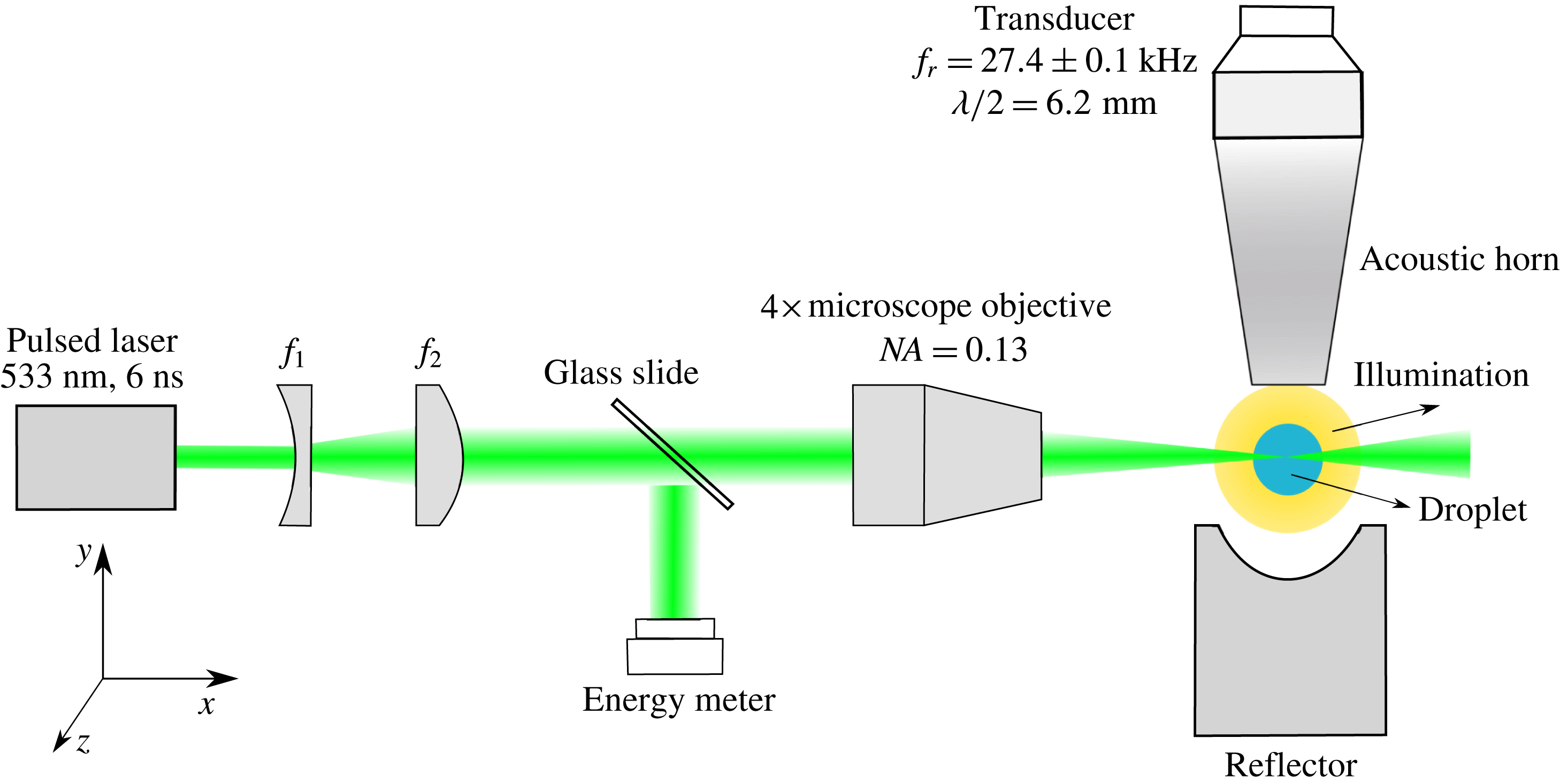
In the experiments, a single millimetre-sized droplet is levitated with a standing-wave acoustic field. The expansion of the droplet is induced by nucleating a cavitation bubble inside the droplet with a pulsed and focused laser: see figure 2. The transducer at the top and the spherical reflector create a standing wave at a frequency of
 $27.4\pm 0.1~\text{kHz}$
. The balance of gravity, acoustic forces and surface tension shapes the droplet into an approximate ellipsoid (Shi & Apfel Reference Shi and Apfel1996; Yarin, Pfaffenlehner & Tropea Reference Yarin, Pfaffenlehner and Tropea1998). The equivalent radius
 $R_{d,eq}$
is the radius of a sphere with the same volume as this ellipsoid. Considering the axisymmetric shape of the droplet (
 $R_{d,x}=R_{d,z}$
), we have
 $R_{d,eq}=(R_{d,x}^{2}R_{d,y})^{1/3}$
, where
 $R_{d,x}$
,
 $R_{d,y}$
and
 $R_{d,z}$
are the semi-principal axis in the
 $x$
,
 $y$
and
 $z$
directions, respectively. Their ratio can be modified within range by varying the amplitude of the acoustic field. An Nd:YAG laser pulse (532 nm wavelength, 6 ns duration) is first collimated with a telescope consisting of a plano-concave and a plano-convex lens (
 $f_{1}$
and
 $f_{2}$
in figure 2) and then focused with a
 $4\times$
microscope objective into the droplet. The laser energy deposited inside the droplet is estimated by sampling approximately 4 % of the original laser pulse energy, as shown in figure 2. A high-speed camera records the experiment while the illumination is provided with an LED powered fibre optic (REVOX SLG 150V). The camera and laser are triggered and synchronized with a signal delay generator. Experimental details are described in Gonzalez-Avila & Ohl (Reference Gonzalez-Avila and Ohl2016).
Experimental set-up.

2.2 CFD simulation
The CFD simulations of the droplet interface are done based on the OpenFOAM framework (Weller et al. Reference Weller, Tabor, Jasak and Fureby1998) by solving the compressible Navier–Stokes equations with the finite volume method (FVM) and using a volume of fluid (VOF) based method for interface capturing. The laser-induced cavitation bubble is modelled as a non-condensable gas starting from a small volume at a high pressure. The gas and liquid phases are treated as compressible and immiscible Newtonian fluids while neglecting heat and mass transfer. Thus, we solve the equation of continuity together with the compressible Navier–Stokes equations:
 $$\begin{eqnarray}\displaystyle & \displaystyle \frac{\unicode[STIX]{x2202}\unicode[STIX]{x1D70C}}{\unicode[STIX]{x2202}t}+\unicode[STIX]{x1D735}\boldsymbol{\cdot }(\unicode[STIX]{x1D70C}\boldsymbol{u})=0, & \displaystyle\end{eqnarray}$$
 $$\begin{eqnarray}\displaystyle & \displaystyle \frac{\unicode[STIX]{x2202}\unicode[STIX]{x1D70C}\boldsymbol{u}}{\unicode[STIX]{x2202}t}+\unicode[STIX]{x1D735}\boldsymbol{\cdot }(\unicode[STIX]{x1D70C}\boldsymbol{u}\boldsymbol{u})=-\unicode[STIX]{x1D735}p+\unicode[STIX]{x1D735}\boldsymbol{\cdot }\unicode[STIX]{x1D749}+\boldsymbol{f}_{\unicode[STIX]{x1D739}}, & \displaystyle\end{eqnarray}$$
where
 $\unicode[STIX]{x1D70C}$
is the density of the fluid,
 $\boldsymbol{u}$
the velocity field,
 $p$
the pressure and
 $\unicode[STIX]{x1D749}$
the viscous stress tensor which is calculated as
 $\unicode[STIX]{x1D749}=\unicode[STIX]{x1D707}[\unicode[STIX]{x1D735}\boldsymbol{u}+\unicode[STIX]{x1D735}\boldsymbol{u}^{\text{T}}-2/3(\unicode[STIX]{x1D735}\boldsymbol{\cdot }\boldsymbol{u})\unicode[STIX]{x1D644}]$
.
 $\unicode[STIX]{x1D644}$
is the identity tensor and
 $\boldsymbol{f}_{\unicode[STIX]{x1D739}}$
the source term due to surface tension which is modelled according to the so-called continuous-surface-force (CSF) method (Brackbill, Kothe & Zemach Reference Brackbill, Kothe and Zemach1992). Gravity and the external acoustic fields are not accounted for. We assume an adiabatic process and relate the gas density to pressure with the Noble–Abel equation of state (EOS) (see Koch et al.
Reference Koch, Lechner, Reuter, Köhler, Mettin and Lauterborn2016):
 $$\begin{eqnarray}\displaystyle p\left(\frac{1}{\unicode[STIX]{x1D70C}_{g}}-\frac{\unicode[STIX]{x1D6FD}}{\unicode[STIX]{x1D70C}_{n}}\right)^{\unicode[STIX]{x1D6FE}}=p_{n}\left(\frac{1}{\unicode[STIX]{x1D70C}_{n}}-\frac{\unicode[STIX]{x1D6FD}}{\unicode[STIX]{x1D70C}_{n}}\right)^{\unicode[STIX]{x1D6FE}}, & & \displaystyle\end{eqnarray}$$
where
 $\unicode[STIX]{x1D70C}_{g}$
is the density of the gas,
 $\unicode[STIX]{x1D70C}_{n}$
and
 $p_{n}$
are the density and pressure for a small bubble of radius
 $R_{n}$
in an equilibrium state,
 $\unicode[STIX]{x1D6FD}$
is the co-volume coefficient, which accounts for the available volume for molecular motion, and
 $\unicode[STIX]{x1D6FE}$
is the specific heat ratio or adiabatic exponent.
For the liquid phase the Tait EOS is applied:
 $$\begin{eqnarray}\displaystyle p=(p_{0}+B)\left(\frac{\unicode[STIX]{x1D70C}_{l}}{\unicode[STIX]{x1D70C}_{0}}\right)^{\unicode[STIX]{x1D6E4}}-B, & & \displaystyle\end{eqnarray}$$
where
 $\unicode[STIX]{x1D70C}_{l}$
is the liquid density,
 $p_{0}$
and
 $\unicode[STIX]{x1D70C}_{0}$
are the reference density and reference pressure, respectively.
 $\unicode[STIX]{x1D6E4}$
is the Tait exponent and
 $B$
the Tait pressure. The parameters are chosen to be the same as in Koch et al. (Reference Koch, Lechner, Reuter, Köhler, Mettin and Lauterborn2016) and are listed in table 1.
The parameter used in the EOS for the gas and the liquid.

The governing equations are solved in a single-field formulation for both phases including the interface cells. In order to capture the interface, the VOF method is used. The indicator function
 $\unicode[STIX]{x1D6FC}$
is defined as the volume fraction of one of the phases, which is solved with a transport equation. For convenience, we introduce instead two volume fraction functions,
 $\unicode[STIX]{x1D6FC}_{l}$
for the liquid phase,
 $$\begin{eqnarray}\displaystyle \unicode[STIX]{x1D6FC}_{l}=\left\{\begin{array}{@{}ll@{}}1, & \text{liquid,}\\ 0, & \text{gas,}\\ 0<\unicode[STIX]{x1D6FC}_{l}<1, & \text{interface,}\end{array}\right. & & \displaystyle\end{eqnarray}$$
and
 $\unicode[STIX]{x1D6FC}_{g}$
for the gas phase,
 $$\begin{eqnarray}\displaystyle \unicode[STIX]{x1D6FC}_{g}=1-\unicode[STIX]{x1D6FC}_{l}. & & \displaystyle\end{eqnarray}$$
Considering the mass conservation for each phase we obtain
 $$\begin{eqnarray}\left.\begin{array}{@{}c@{}}\displaystyle \frac{\unicode[STIX]{x2202}\unicode[STIX]{x1D70C}_{l}\unicode[STIX]{x1D6FC}_{l}}{\unicode[STIX]{x2202}t}+\unicode[STIX]{x1D735}\boldsymbol{\cdot }(\unicode[STIX]{x1D70C}_{l}\boldsymbol{u}\unicode[STIX]{x1D6FC}_{l})=0,\\ \displaystyle \frac{\unicode[STIX]{x2202}\unicode[STIX]{x1D70C}_{g}\unicode[STIX]{x1D6FC}_{g}}{\unicode[STIX]{x2202}t}+\unicode[STIX]{x1D735}\boldsymbol{\cdot }(\unicode[STIX]{x1D70C}_{g}\boldsymbol{u}\unicode[STIX]{x1D6FC}_{g})=0.\end{array}\right\}\end{eqnarray}$$
Rewriting (2.7) and introducing the compressibility
 $\unicode[STIX]{x1D713}=\text{D}\unicode[STIX]{x1D70C}/\text{D}p$
from the EOS, we obtain an evolution equation for the liquid volume fraction,
 $$\begin{eqnarray}\displaystyle \frac{\unicode[STIX]{x2202}\unicode[STIX]{x1D6FC}_{l}}{\unicode[STIX]{x2202}t}+\unicode[STIX]{x1D735}\boldsymbol{\cdot }(\unicode[STIX]{x1D6FC}_{l}\boldsymbol{u})+\unicode[STIX]{x1D735}\boldsymbol{\cdot }(\unicode[STIX]{x1D6FC}_{l}\unicode[STIX]{x1D6FC}_{g}\boldsymbol{U}_{\boldsymbol{r}})=\unicode[STIX]{x1D6FC}_{l}\unicode[STIX]{x1D6FC}_{g}\left(\frac{\unicode[STIX]{x1D713}_{g}}{\unicode[STIX]{x1D70C}_{g}}-\frac{\unicode[STIX]{x1D713}_{l}}{\unicode[STIX]{x1D70C}_{l}}\right)\frac{\text{D}p}{\text{D}t}+\unicode[STIX]{x1D6FC}_{l}\unicode[STIX]{x1D735}\boldsymbol{\cdot }\boldsymbol{u}, & & \displaystyle\end{eqnarray}$$
where
 $\boldsymbol{U}_{\boldsymbol{r}}$
is the relative velocity between the two phases. From (2.8) we see that
 $\boldsymbol{U}_{\boldsymbol{r}}$
acts as an artificial compressibility which helps to ensure a sharp interface (Rusche Reference Rusche2003). This relative velocity is determined from the normal vector of the cell surface
 $\boldsymbol{n}_{\boldsymbol{f}}$
, the cell surface area
 $S_{f}$
, the volume flux
 $\unicode[STIX]{x1D719}_{f}$
and an adjustable compression coefficient
 $C_{f}$
between 0 and 1:
 $$\begin{eqnarray}\displaystyle \boldsymbol{U}_{\boldsymbol{r}}=\boldsymbol{n}_{\boldsymbol{f}}C_{f}\frac{|\unicode[STIX]{x1D719}_{f}|}{|S_{f}|}. & & \displaystyle\end{eqnarray}$$
The surface tension source term
 $\boldsymbol{f}_{\unicode[STIX]{x1D739}}$
is obtained from
 $$\begin{eqnarray}\displaystyle f_{\unicode[STIX]{x1D6FF}}=\unicode[STIX]{x1D70E}\left[-\unicode[STIX]{x1D735}\boldsymbol{\cdot }\left(\frac{\unicode[STIX]{x1D735}\unicode[STIX]{x1D6FC}_{l}}{|\unicode[STIX]{x1D735}\unicode[STIX]{x1D6FC}_{l}|}\right)\right]\unicode[STIX]{x1D735}\unicode[STIX]{x1D6FC}_{l}, & & \displaystyle\end{eqnarray}$$
where
 $\unicode[STIX]{x1D70E}$
is the coefficient of surface tension. Physical parameters depending on the void fraction,
 $\unicode[STIX]{x1D702}$
such as viscosity or density are calculated through
 $$\begin{eqnarray}\displaystyle \unicode[STIX]{x1D702}=\unicode[STIX]{x1D702}_{l}\unicode[STIX]{x1D6FC}_{l}+\unicode[STIX]{x1D702}_{g}\unicode[STIX]{x1D6FC}_{g}, & & \displaystyle\end{eqnarray}$$
where
 $\unicode[STIX]{x1D702}_{l}$
and
 $\unicode[STIX]{x1D702}_{g}$
are the parameters for liquid and gas phases respectively. The viscosities are constant in each of the phase while densities are updated based on the equations of state.
Considering the compressibility, the continuity equation (2.7) can be re-written as
 $$\begin{eqnarray}\displaystyle \left(\frac{\unicode[STIX]{x1D6FC}_{l}}{\unicode[STIX]{x1D70C}_{l}}\unicode[STIX]{x1D713}_{l}+\frac{\unicode[STIX]{x1D6FC}_{g}}{\unicode[STIX]{x1D70C}_{g}}\unicode[STIX]{x1D713}_{g}\right)\frac{\text{D}p}{\text{D}t}+\unicode[STIX]{x1D735}\boldsymbol{\cdot }\boldsymbol{u}=0. & & \displaystyle\end{eqnarray}$$
Here the PIMPLE algorithm solves the pressure–velocity coupling in the momentum equation (Greenshields Reference Greenshields2015), which is a combination of the PISO (pressure-implicit split-operator) and the SIMPLE (semi-implicit method for pressure-linked equations) algorithms. The volume fraction equation in the VOF method is solved using a MULES (multi-dimensional universal limiter with explicit solution) algorithm (Rusche Reference Rusche2003; Greenshields Reference Greenshields2015) and an AIC (artificial interface compression) algorithm to ensure the sharp interface without geometry reconstruction (Ubbink Reference Ubbink1997). The time step is adaptively changed depending on the Courant number to ensure the stability of the solution. In short the solution is obtained through the following steps.
(i) Solve VOF transport equation (2.8) to get
 $\unicode[STIX]{x1D6FC}_{l}$
and
$\unicode[STIX]{x1D6FC}_{g}$
.
(ii) Update the material properties according to
$\unicode[STIX]{x1D6FC}_{l}$
for the first correction of one PIMPLE loop.(iii) Update density according to equation of continuity (2.1).
(iv) Solve momentum equation (2.2) and the pressure equation (2.12).
(v) Compute compressibility and densities from state equations (2.3) and (2.4).


Every time step is treated as a PIMPLE algorithm loop, and all of the above steps are repeated for each loop until the simulation end time is reached. The temporal derivatives are discretized using the implicit Euler scheme. A second-order van Leer scheme and a second-order upwind scheme are applied to discretize the convective terms in the volume fraction equation and in the momentum equation, respectively. For the other terms a second-order Gauss linear difference scheme is used.
2.3 Stability analysis
Here we model the Rayleigh–Taylor stability of the droplet’s spherical surface, i.e. the stability of the surface from which the jets are ejected. As sketched in figure 1(b), the droplet is a sphere of radius
 $R$
, density
 $\unicode[STIX]{x1D70C}_{1}$
and dynamic viscosity
 $\unicode[STIX]{x1D707}_{1}$
; the outer interface is surrounded by a lighter fluid with density
 $\unicode[STIX]{x1D70C}_{2}$
and dynamic viscosity
 $\unicode[STIX]{x1D707}_{2}$
, i.e. the surrounding gas. The droplet and the surrounding gas are treated as immiscible and incompressible fluids. The interface position, i.e. the droplet radius
 $R$
is a function of time, in particular the surface is susceptible to a radial acceleration driven by the internal bubble. This may lead to the growth of surface perturbations.
The surface perturbations are modelled as a spherical harmonic
 $Y_{n}$
with mode
 $n$
, i.e.
 $r_{s}(t)=R(t)+a(t)Y_{n}$
, where
 $a(t)$
is the amplitude of the perturbations, starting from some small initial value
 $|a(t=0)|\ll R(t=0)$
. The evolution equation of this perturbation amplitude to the first order has been derived by Prosperetti (Reference Prosperetti1977) for incompressible and viscous spherical flows:
 $$\begin{eqnarray}\displaystyle & & \displaystyle \left(\frac{\unicode[STIX]{x1D70C}_{2}}{n+1}+\frac{\unicode[STIX]{x1D70C}_{1}}{n}\right)R\ddot{a}+\left[3\left(\frac{\unicode[STIX]{x1D70C}_{2}}{n+1}+\frac{\unicode[STIX]{x1D70C}_{1}}{n}\right){\dot{R}}-\frac{2}{R}(n+2)(n-1)(\unicode[STIX]{x1D707}_{2}-\unicode[STIX]{x1D707}_{1})\right]{\dot{a}}\nonumber\\ \displaystyle & & \displaystyle \quad +\,\left[\left(\frac{n+2}{n}\unicode[STIX]{x1D70C}_{1}-\frac{n-1}{n+1}\unicode[STIX]{x1D70C}_{2}\right)\ddot{R}+2(n-1)(n+2)(\unicode[STIX]{x1D707}_{2}-\unicode[STIX]{x1D707}_{1})\frac{{\dot{R}}}{R^{2}}+(n-1)(n+2)\frac{\unicode[STIX]{x1D70E}}{R^{2}}\right]a\nonumber\\ \displaystyle & & \displaystyle \quad +\,n(n+2)\unicode[STIX]{x1D707}_{2}\frac{T_{2}(R,t)}{R}-(n+1)(n-1)\unicode[STIX]{x1D707}_{1}\frac{T_{1}(R,t)}{R}\nonumber\\ \displaystyle & & \displaystyle \quad +\,(n+1)\unicode[STIX]{x1D70C}_{1}\frac{{\dot{R}}}{R}\int _{0}^{R}\left[1-\left(\frac{s}{R}\right)^{3}\right]\left(\frac{s}{R}\right)^{n-2}T_{1}(s,t)\,\text{d}s\nonumber\\ \displaystyle & & \displaystyle \quad -\,n\unicode[STIX]{x1D70C}_{2}\frac{{\dot{R}}}{R}\int _{R}^{\infty }\left[1-\left(\frac{R}{s}\right)^{3}\right]\left(\frac{R}{s}\right)^{n}T_{2}(s,t)\,\text{d}s=0.\end{eqnarray}$$
Here
 $\unicode[STIX]{x1D70E}$
is the coefficient of surface tension,
 $T_{1}(r,t)$
and
 $T_{2}(r,t)$
are the terms related to viscous effects for the liquid region and the surrounding gas region respectively, which we discuss later. For convenience and due to the large ratio of density and viscosity i.e.
 $\unicode[STIX]{x1D70C}_{1}\gg \unicode[STIX]{x1D70C}_{2}$
and
 $\unicode[STIX]{x1D707}_{1}\gg \unicode[STIX]{x1D707}_{2}$
, we neglect the air density and viscosity and use
 $\unicode[STIX]{x1D70C}=\unicode[STIX]{x1D70C}_{1}$
,
 $\unicode[STIX]{x1D707}=\unicode[STIX]{x1D707}_{1}$
and
 $T(r,t)=T_{1}(r,t)$
to denote the only relevant liquid properties. The perturbation equation (2.13) can then be simplified to
 $$\begin{eqnarray}\displaystyle & & \displaystyle \ddot{a}+B_{n}(t){\dot{a}}-A_{n}(t)a-(n-1)n(n+1)\frac{\unicode[STIX]{x1D707}}{\unicode[STIX]{x1D70C}R^{2}}T(R,t)\nonumber\\ \displaystyle & & \displaystyle \qquad +\,n(n+1)\frac{{\dot{R}}}{R}\int _{0}^{R}\left[1-\left(\frac{s}{R}\right)^{3}\right]\left(\frac{s}{R}\right)^{n-2}T(s,t)\,\text{d}s=0,\end{eqnarray}$$
with
 $$\begin{eqnarray}\displaystyle A_{n}(t)=-(n+2)\frac{\ddot{R}}{R}-(n-1)n(n+2)\frac{\unicode[STIX]{x1D70E}}{\unicode[STIX]{x1D70C}R^{3}}+(n-1)n(n+2)\frac{2\unicode[STIX]{x1D707}{\dot{R}}}{\unicode[STIX]{x1D70C}R^{3}} & & \displaystyle\end{eqnarray}$$
and
 $$\begin{eqnarray}\displaystyle B_{n}(t)=\frac{3{\dot{R}}}{R}+\frac{2(n-1)n(n+2)\unicode[STIX]{x1D707}}{\unicode[STIX]{x1D70C}R^{2}}. & & \displaystyle\end{eqnarray}$$
The
 $T(r,t)$
is a toroidal component of the vorticity
 $\unicode[STIX]{x1D714}$
produced by the viscous stress near the surface. The vorticity
 $\unicode[STIX]{x1D714}$
is decomposed into a poloidal scalar field
 $S(r,t)$
and a toroidal scalar field
 $T(r,t)$
:
 $$\begin{eqnarray}\displaystyle \unicode[STIX]{x1D714}=\unicode[STIX]{x1D735}\times \unicode[STIX]{x1D735}\times [S(r,t)Y_{n}^{m}(\unicode[STIX]{x1D703},\unicode[STIX]{x1D719})\boldsymbol{e}_{r}]+\unicode[STIX]{x1D735}\times [T(r,t)Y_{n}^{m}(\unicode[STIX]{x1D703},\unicode[STIX]{x1D719})\boldsymbol{e}_{r}]. & & \displaystyle\end{eqnarray}$$
The poloidal part
 $S(r,t)$
is needed only to satisfy the particular initial conditions during the brief initial time of the dynamic problem, which is neglected in our case. In contrast the toroidal part
 $T(r,t)$
is the main contribution to the vorticity. Its evolution according to Prosperetti (Reference Prosperetti1977) and Hilgenfeldt et al. (Reference Hilgenfeldt, Lohse and Brenner1996) is
 $$\begin{eqnarray}\displaystyle \frac{\unicode[STIX]{x1D707}}{\unicode[STIX]{x1D70C}}\frac{\unicode[STIX]{x2202}^{2}T(r,t)}{\unicode[STIX]{x2202}r^{2}}-\frac{\unicode[STIX]{x2202}T}{\unicode[STIX]{x2202}t}-\frac{\unicode[STIX]{x2202}}{\unicode[STIX]{x2202}r}\left[\left(\frac{R}{r}\right)^{2}{\dot{R}}\,T(r,t)-\frac{\unicode[STIX]{x1D707}n(n+1)}{\unicode[STIX]{x1D70C}r^{2}}T(r,t)\right]=0. & & \displaystyle\end{eqnarray}$$
The boundary condition for
 $T(r,t)$
is the continuity of tangential stresses to first order in
 $a$
(Prosperetti Reference Prosperetti1977; Hilgenfeldt et al.
Reference Hilgenfeldt, Lohse and Brenner1996), i.e.
 $$\begin{eqnarray}\displaystyle T(R,t)-2R^{-n-2}\int _{0}^{R}s^{n+1}T(s,t)\,\text{d}s=\frac{2}{n}\left[(n+1){\dot{a}}-(n+2)\frac{{\dot{R}}}{R}a\right]. & & \displaystyle\end{eqnarray}$$
The second boundary condition is
 $T(R=0,t)=0$
.
Equations (2.14)–(2.19) are a complete set of equations for the stability analysis, yet it contains an integral
 $T(R,t)$
. The vorticity is only considered to be generated within a small boundary layer of thickness
 $\unicode[STIX]{x1D6FF}$
near the droplet–gas interface. We therefore can approximate the integral term in (2.14) with
 $$\begin{eqnarray}\displaystyle \int _{0}^{R}\left[1-\left(\frac{s}{R}\right)^{3}\right]\left(\frac{s}{R}\right)^{n-2}T(s,t)\,\text{d}s\approx \unicode[STIX]{x1D6FF}\left[1-\left(\frac{s}{R}\right)^{3}\right]\left(\frac{s}{R}\right)^{n-2}\left.T(s,t)\right|_{s=R}=0, & & \displaystyle\end{eqnarray}$$
and in (2.19) with
 $$\begin{eqnarray}\displaystyle R^{-n-2}\int _{0}^{R}s^{n+1}T(s,t)\,\text{d}s\approx R^{-n-2}[R^{n+1}T(R,t)\unicode[STIX]{x1D6FF}]=\frac{\unicode[STIX]{x1D6FF}}{R}T(R,t). & & \displaystyle\end{eqnarray}$$
Combining (2.19) and (2.21) we obtain an expression for
 $$\begin{eqnarray}\displaystyle T(R,t)=\frac{1}{1-\displaystyle \frac{2\unicode[STIX]{x1D6FF}}{R}}\frac{2}{n}\left[(n+1){\dot{a}}-(n+2)\frac{{\dot{R}}}{R}a\right]. & & \displaystyle\end{eqnarray}$$
Since the droplet radius
 $R(t)$
is much larger than the boundary layer
 $\unicode[STIX]{x1D6FF}$
, i.e.
 $R\gg \unicode[STIX]{x1D6FF}$
,
 $T(R,t)$
is approximated as
 $$\begin{eqnarray}\displaystyle T(R,t)\approx \frac{2}{n}\left[(n+1){\dot{a}}-(n+2)\frac{{\dot{R}}}{R}a\right]. & & \displaystyle\end{eqnarray}$$
Combining the above equations we obtain
 $$\begin{eqnarray}\displaystyle \ddot{a}+B_{n}(t){\dot{a}}-A_{n}(t)a=0, & & \displaystyle\end{eqnarray}$$
with
 $$\begin{eqnarray}\displaystyle A_{n}(t)=-(n+2)\frac{\ddot{R}}{R}-(n-1)n(n+2)\frac{\unicode[STIX]{x1D70E}}{\unicode[STIX]{x1D70C}R^{3}}-(n-1)(n+2)\frac{2\unicode[STIX]{x1D707}{\dot{R}}}{\unicode[STIX]{x1D70C}R^{3}}, & & \displaystyle\end{eqnarray}$$
and
 $$\begin{eqnarray}\displaystyle B_{n}(t)=\frac{3{\dot{R}}}{R}+\frac{2(n-1)(2n+1)\unicode[STIX]{x1D707}}{\unicode[STIX]{x1D70C}R^{2}}. & & \displaystyle\end{eqnarray}$$
To solve the perturbation equation (2.24), the droplet radius
 $R$
, velocity
 ${\dot{R}}$
and acceleration
 $\ddot{R}$
are needed. The droplet radius and velocity are related through
 $$\begin{eqnarray}\displaystyle R^{3}-R_{b}^{3}=R_{0}^{3}-R_{b0}^{3}, & & \displaystyle\end{eqnarray}$$
thus in an incompressible liquid the droplet size and the interface velocity
 $$\begin{eqnarray}\displaystyle R^{2}{\dot{R}}=R_{b}^{2}\dot{R_{b}}, & & \displaystyle\end{eqnarray}$$
are uniquely define through the bubble radius and the constant volume of the droplet. Here
 $R$
and
 $R_{b}$
are the time varying radii of the droplet and the bubble,
 $R_{0}$
and
 $R_{b0}$
are the initial droplet and bubble radii and
 ${\dot{R}}$
and
 $\dot{R_{b}}$
are the radial velocities of the droplet and the bubble, respectively.
The bubble dynamics is obtained from the unsteady Bernoulli equation similar to Obreschkow et al. (Reference Obreschkow, Kobel, Dorsaz, De Bosset, Nicollier and Farhat2006),
 $$\begin{eqnarray}\displaystyle \frac{P_{b}-P_{\infty }}{\unicode[STIX]{x1D70C}}=\frac{3}{2}{{\dot{R}}_{b}}^{2}+R_{b}\ddot{R}_{b}+\frac{4\unicode[STIX]{x1D707}}{R_{b}\unicode[STIX]{x1D70C}}{\dot{R}}_{b}+\frac{2\unicode[STIX]{x1D70E}}{\unicode[STIX]{x1D70C}R_{b}}+\frac{2\unicode[STIX]{x1D70E}}{\unicode[STIX]{x1D70C}R}-2{{\dot{R}}_{b}}^{2}\unicode[STIX]{x1D706}-R_{b}\ddot{R}_{b}\unicode[STIX]{x1D706}+\frac{1}{2}{{\dot{R}}_{b}}^{2}\unicode[STIX]{x1D706}^{4}, & & \displaystyle\end{eqnarray}$$
with
 $$\begin{eqnarray}\displaystyle \unicode[STIX]{x1D706}=R_{b}(t)/R(t), & & \displaystyle\end{eqnarray}$$
and assuming an adiabatic bubble surface,
 $$\begin{eqnarray}\displaystyle P_{b}R_{b}^{3\unicode[STIX]{x1D6FE}}=P_{0}R_{b0}^{3\unicode[STIX]{x1D6FE}}, & & \displaystyle\end{eqnarray}$$
where
 $P_{b}$
is the pressure of the gas in the bubble starting from an initial value of
 $P_{0}$
while
 $P_{\infty }$
is the pressure far from the bubble and
 $\unicode[STIX]{x1D6FE}$
is the ratio of specific heats.
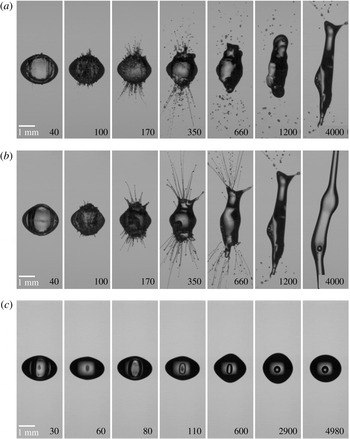
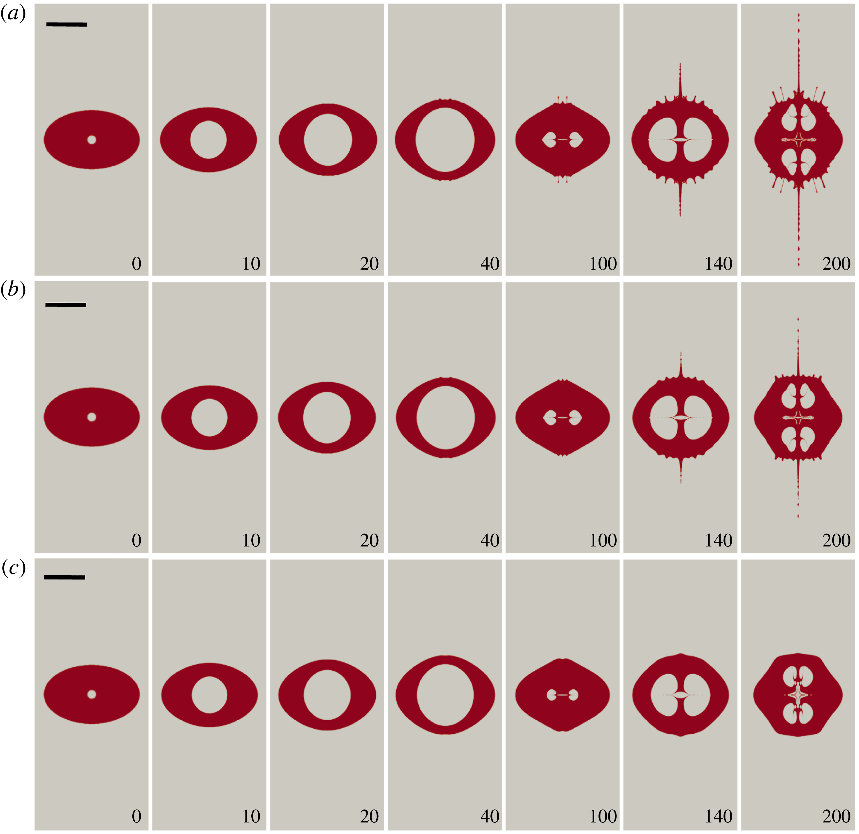
Experimental records of different fluids under similar laser energy: (a) water droplet, laser energy is 2.9 mJ,
 $R_{d,eq}=884~\unicode[STIX]{x03BC}\text{m}$
; (b) 10 cSt silicone oil, laser energy is 2.6 mJ,
 $R_{d,eq}=839~\unicode[STIX]{x03BC}\text{m}$
; (c) 100 cSt silicone oil, laser energy is 2.6 mJ,
 $R_{d,eq}=839~\unicode[STIX]{x03BC}\text{m}$
. Time in
 $\unicode[STIX]{x03BC}\text{s}$
; the scale bar represents 1 mm.

3 Results
3.1 Experiment
We start with a description of the experiments with droplets having different viscosities and undergoing accelerated growth due to internal cavitation. Selected snapshots from high-speed videos recorded at
 $100\,000~\text{frames}~\text{s}^{-1}$
are displayed in figure 3 for three droplets of increasing viscosity: water (1 cSt), 10 cSt silicone oil and 100 cSt silicone oil. They have a similar size and are exposed to a laser pulse of similar energy. The laser-induced cavitation bubbles are nucleated very close to the droplet centre, which ensures the bubble oscillates within an intact droplet while instabilities are excited on the outer surface. We see jets develop in water and in 10 cSt oil droplets; no jets are generated in 100 cSt oil droplets.
During bubble nucleation a shock wave is emitted which reflects at the droplet surface as a rarefaction wave. This reflection may lead to a short-lived Richtmyer–Meshkov instability (Krechetnikov Reference Krechetnikov2009). Additionally, we cannot rule out secondary cavitation generated on an annular ring close to the droplet equator: see Gonzalez-Avila & Ohl (Reference Gonzalez-Avila and Ohl2016). Thus the amplitude of the initial disturbance may be governed by these two processes. The growth of the amplitude occurs only much later and we therefore see the main contribution for jet formation from the Rayleigh–Taylor instability driven by the unsteady flow of the expanding and shrinking bubble.
When jetting occurs surface perturbations on the droplet are already noticeable at maximum bubble expansion (around
 $40~\unicode[STIX]{x03BC}\text{s}$
); they grow during the bubble collapse (around
 $100~\unicode[STIX]{x03BC}\text{s}$
) into thin filaments or jets. The velocity of the jets increases during the second bubble expansion (around
 $170~\unicode[STIX]{x03BC}\text{s}$
) and increase even more during the third expansion of the bubble (around
 $300~\unicode[STIX]{x03BC}\text{s}$
). The 10 cSt oil droplet exhibits a lower number of jets on an overall smoother surface as compared to the water droplet. Moreover, the water jets break up earlier than the oil jets. At a later time,
 $t=4~\text{ms}$
, the droplet has stretched vertically in the direction of the filamentous jets; again the more viscous droplet in 10 cSt extends more than the water case. At higher viscosities, e.g. 100 cSt, surface instabilities are noticeably damped.
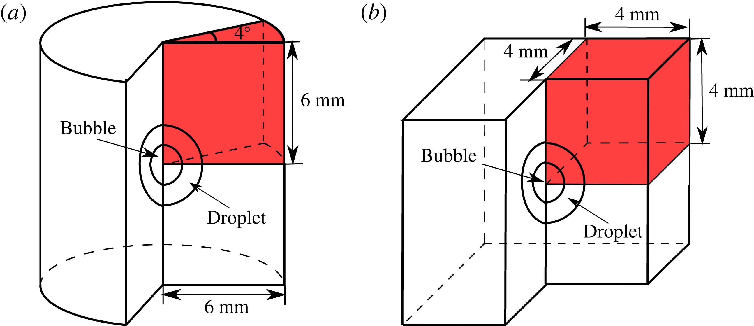
The computational domains. The regions in red are the computational domains used in the simulations considering the symmetry: (a) the domain for 2-D axisymmetric simulation; (b) the domain for 3-D simulation.

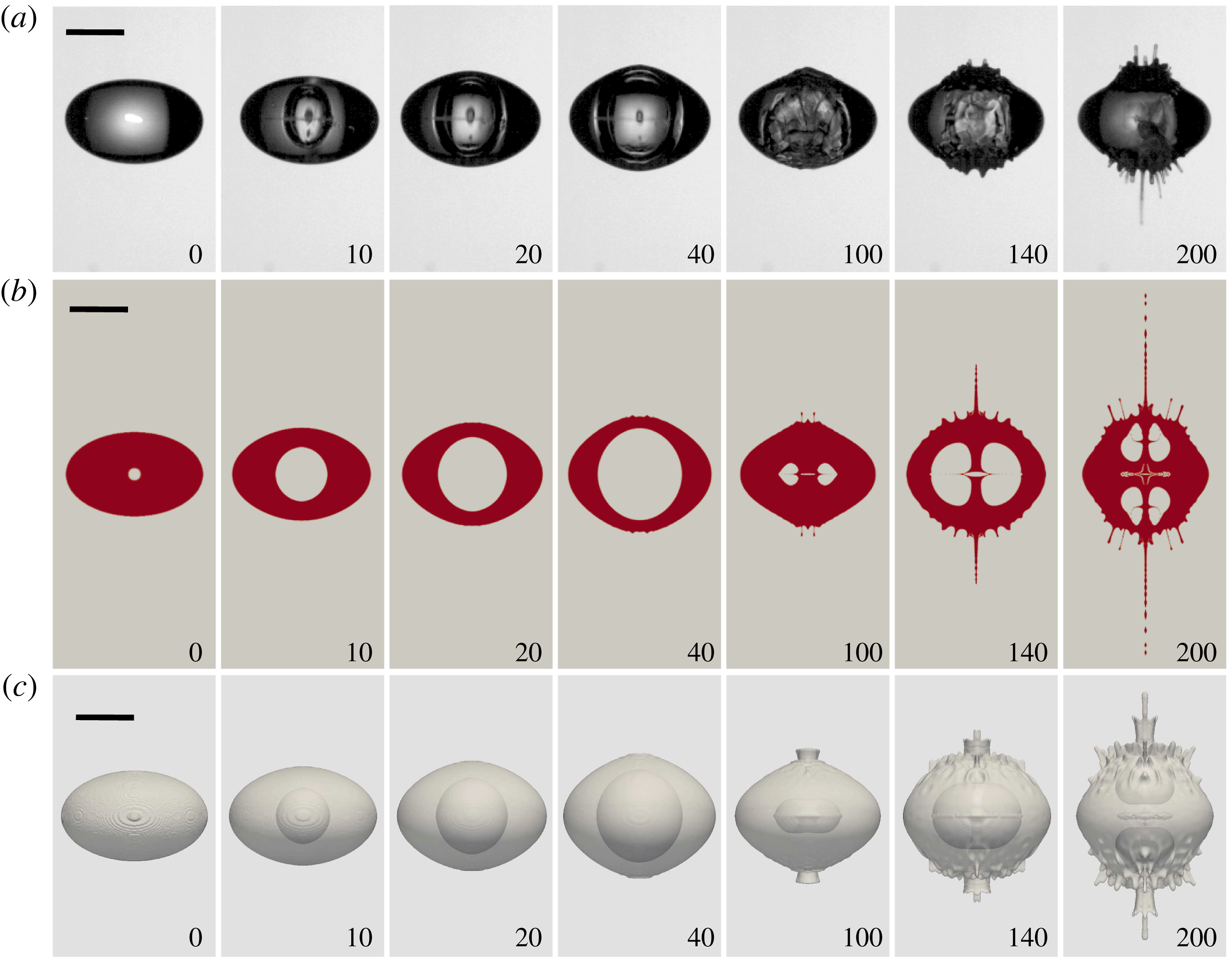
Comparison of experiment, 2-D axisymmetric and 3-D simulation results of water droplet: (a) experiment,
 $R_{d,eq}=1.429~\text{mm}$
, laser energy is 2.2 mJ; (b) 2-D axisymmetric, initial bubble size is
 $100~\unicode[STIX]{x03BC}\text{m}$
, initial bubble pressure is 400 bar; (c) 3-D simulation, same condition as 2-D axisymmetric. Droplets are the same in experiment, 2-D axis axisymmetric simulation, and 3-D simulation. Time in
 $\unicode[STIX]{x03BC}\text{s}$
; the scale bar represents 1 mm.

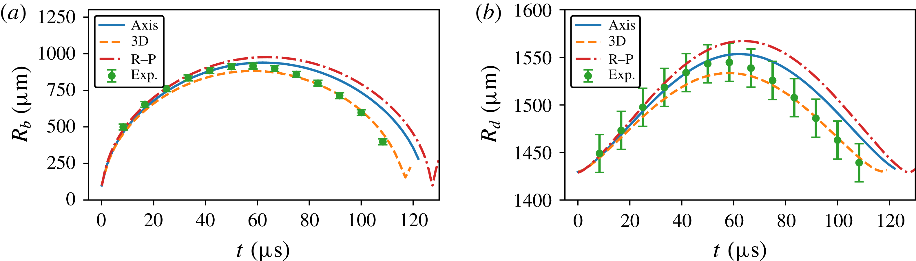
Comparison of the equivalent radius for the water droplet in figure 5. (a) Bubble; (b) droplet. The blue line, orange dashed line and red dash-dot line represent the results from axisymmetric simulation, 3-D simulation and analytic solution (the modified Rayleigh–Plesset equation (2.29)), respectively. Filled symbols are the experimental data. The error from the recorded image is
 $\pm 20~\unicode[STIX]{x03BC}\text{m}$
, which does not take into account the optical distortion.

3.2 Simulation
We now turn to the CFD results: figure 4 shows the domains and figure 5 (see also supplementary movies 1–3 available at https://doi.org/10.1017/jfm.2018.284) compares the experiment of a bubble expanding in a water droplet with simulations done in axisymmetric symmetry and in three dimensions. Initially, the droplet starts as an ellipsoid with semi-principal axes of 1.58 mm, 1.17 mm and 1.58 mm. The laser energy is approximately 2.2 mJ;
 $7.1\pm 4.0\,\%$
of this energy is converted in mechanical energy of the cavitation bubble (Gonzalez-Avila & Ohl Reference Gonzalez-Avila and Ohl2016). In the simulations the complex physics of bubble nucleation is avoided by starting with a spherical bubble with a radius of
 $100~\unicode[STIX]{x03BC}\text{m}$
centred in the droplet. In the axisymmetric simulations, figure 5(b), the domain size is
 $6~\text{mm}\times 6~\text{mm}$
(see figure 4
a), and the computational mesh contains 801 grid points in both radial and vertical directions. For the 3-D simulations only
 $1/8$
th of the ellipsoid is computed to reduce computational time and resources. The domain is
 $4\times 4\times 4~\text{mm}^{3}$
(see figure 4
b), with an unequally distributed mesh with 401 grid points in all directions. The boundary condition of all boundaries except the symmetry boundaries is a vanishing gradient of velocities and stresses that allows for in and out flux. The initial conditions at
 $t=0$
are for the pressure of the surrounding air
 $p=p_{\infty }=1.01315~\text{bar}$
and
 $p=400~\text{bar}$
for the gas in the bubble. This initial bubble pressure and initial bubble radius together reflect the energy in the experiment and we get a similar maximum size of the bubbles. The dynamic viscosity is
 $1\times 10^{-3}~\text{kg}~\text{m}^{-1}~\text{s}^{-1}$
for water and
 $1.84\times 10^{-5}~\text{kg}~\text{m}^{-1}~\text{s}^{-1}$
for the surrounding air and the coefficient of surface tension is
 $\unicode[STIX]{x1D70E}=0.0728~\text{N}~\text{m}^{-1}$
.
A comparison of the bubble and droplet radius for the axisymmetric and 3-D CFD simulations, the Rayleigh–Plesset solution and the experiment for the water droplet as shown in figure 5 is provided in figure 6. The initial radius of the cavitation bubble is set to
 $100~\unicode[STIX]{x03BC}\text{m}$
, which is approximately the size of the plasma spot. By adjusting the initial pressure in the simulations we can achieve a similar maximum size of the bubbles: these are
 $916~\unicode[STIX]{x03BC}\text{m}$
,
 $939~\unicode[STIX]{x03BC}\text{m}$
,
 $881~\unicode[STIX]{x03BC}\text{m}$
and
 $976~\unicode[STIX]{x03BC}\text{m}$
in experiment, axisymmetric simulation, 3-D simulation and the analytic solution, respectively. The pressure at maximum expansion in the CFD simulations is approximately 3.9 kPa. The 3-D simulation results provide the best agreement with the experiments while the results from the axisymmetric simulation and analytic solution are very close.
In figure 5 we focus on the first
 $300~\unicode[STIX]{x03BC}\text{s}$
of the bubble oscillation covering three oscillation cycles with two bubble rebounds. The axisymmetric simulation in figure 5(b) is presented as a cut through the centre of the droplet, showing clearly the shape of the droplet and bubble. In axisymmetry these perturbations are not column-like jets but annular surfaces. To compare more closely the shape of the jets with experiments, 3-D simulations are shown in figure 5(c). Overall, we find very good agreement between the simulations and experiments, in particular the onset of disturbances and their velocity. Also, the bubble dynamics is covered up to the first collapse around
 $t\approx 117~\unicode[STIX]{x03BC}\text{s}$
, thereafter the corrugated droplet’s surface does not allow a closer look at the cavitation bubble in the experiments.
Let us first compare the experiment in figure 5(a), with the cut plane of the 2-D simulation as shown in figure 5(b). The cavitation bubble expands and reaches a maximum volume at
 $t\approx 50~\unicode[STIX]{x03BC}\text{s}$
and collapses around
 $117~\unicode[STIX]{x03BC}\text{s}$
. As the bubble expands and shrinks, the droplet volume changes mostly along the vertical direction which is the direction of lowest inertia. Around
 $t\approx 117~\unicode[STIX]{x03BC}\text{s}$
the bubble collapses into an approximate toroidal shape (figure 5
a); in the simulations also a torus is found forming during the re-expansion (figure 5
b). This is the result of the bubble growing while two jets from the top and bottom of the droplet are accelerating to the droplet centre. Even before the bubble collapses some roughness on the droplet surface is visible, starting at the upper and lower poles at
 $t=50~\unicode[STIX]{x03BC}\text{s}$
in the experiment and simulations. The ripples develop into thin ligaments during the second expansion. During this process the crests on the surface convert into troughs which we explain below with the specific time varying radial acceleration. The ligaments are formed at
 $t=300~\unicode[STIX]{x03BC}\text{s}$
all over the droplet surface both in experiments and in the simulations, yet they are fastest at both poles, at places closest to the bubble which are also the places of highest acceleration. Overall, the growth of the perturbations on the droplet surface during the bubble expansion possesses some similarity to the formation of jets under impulsive acceleration of a curved free surface (Antkowiak et al.
Reference Antkowiak, Bremond, Le Dizès and Villermaux2007). The obvious difference in our present experiment is that the initial interface is convex. Yet the initial perturbation generated by the Rayleigh–Taylor instability transforms the globally convex (ellipsoidal) interface into a locally concave interface.
The 3-D simulation in figure 5(c) depicts overall a very similar scenario to the 2-D simulations and excellent agreement with the experiment. The bubble collapses slightly faster, showing a smaller volume at
 $t=117~\unicode[STIX]{x03BC}\text{s}$
than the 2-D simulations. The biggest advantage of the 3-D simulation is that the jets are thin ligaments, as observed in the experiments.
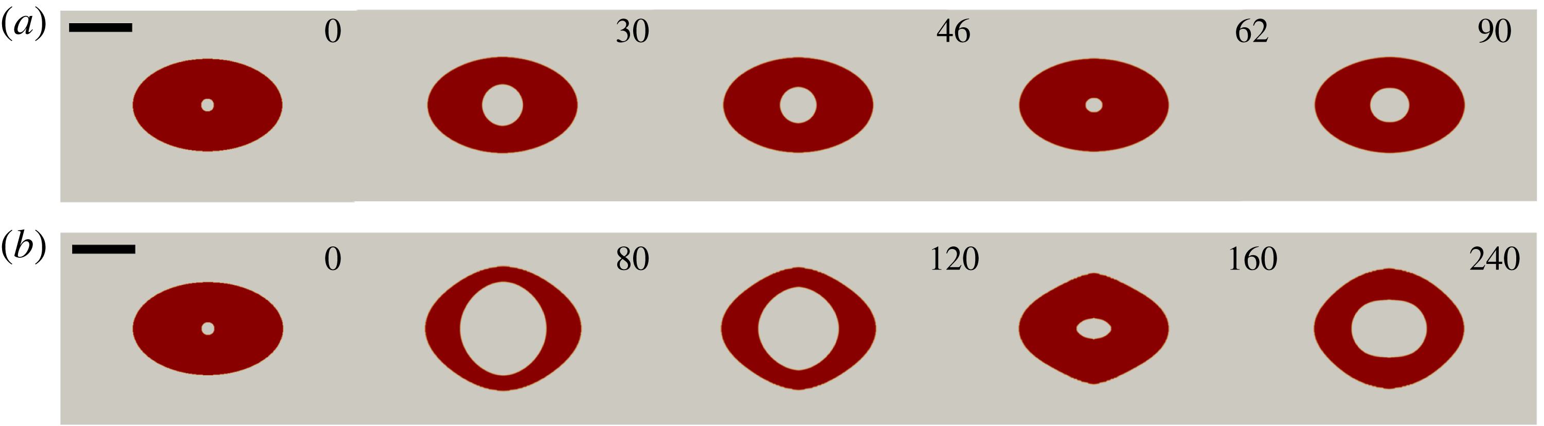
Comparison of experiment, 2-D axisymmetric and 3-D simulation results of 10 cSt silicone oil droplet: (a) experiment,
 $R_{d,eq}=1.02~\text{mm}$
, laser energy is 1.4 mJ; (b) 2-D axisymmetric, initial bubble size is
 $100~\unicode[STIX]{x03BC}\text{m}$
, initial bubble pressure is 250 bar; (c) 3-D simulation, same condition as 2-D axisymmetric. Droplets are the same in experiment, 2-D axis axisymmetric simulation and 3-D simulation. Time in
 $\unicode[STIX]{x03BC}\text{s}$
; the scale bar represents 1 mm.

A second comparison of the simulations with an experiment is shown in figure 7 for a droplet with 10 times higher viscosity, i.e.
 $\unicode[STIX]{x1D707}_{l}=10^{-2}~\text{Pa}~\text{s}$
,
 $\unicode[STIX]{x1D70C}_{l}=10^{3}~\text{kg}~\text{m}^{-3}$
and
 $\unicode[STIX]{x1D70E}=0.02~\text{N}~\text{m}^{-1}$
. We find overall agreement and a dynamics resembling the water case as shown in figure 5. Yet on a closer look we notice that the axisymmetric simulation (figure 7
b) predicts a faster jet along the centre of symmetry. Starting from
 $t=140~\unicode[STIX]{x03BC}\text{s}$
after the first collapse there are some differences in the overall shape of the droplet. The droplet is stretched more in the horizontal direction than in the simulation. This may be caused by the dominance of the acoustic forces (Foresti, Nabavi & Poulikakos Reference Foresti, Nabavi and Poulikakos2012) which are not accounted for in the simulations. Interestingly, the jetting in the experiment is more closely predicted with the 3-D simulations (figure 7
c). Overall, the effect of viscosity is the reduction of surface ripples during the first bubble expansion and collapse leading to jets closer to the poles and a smoother interface along the droplet’s equator.
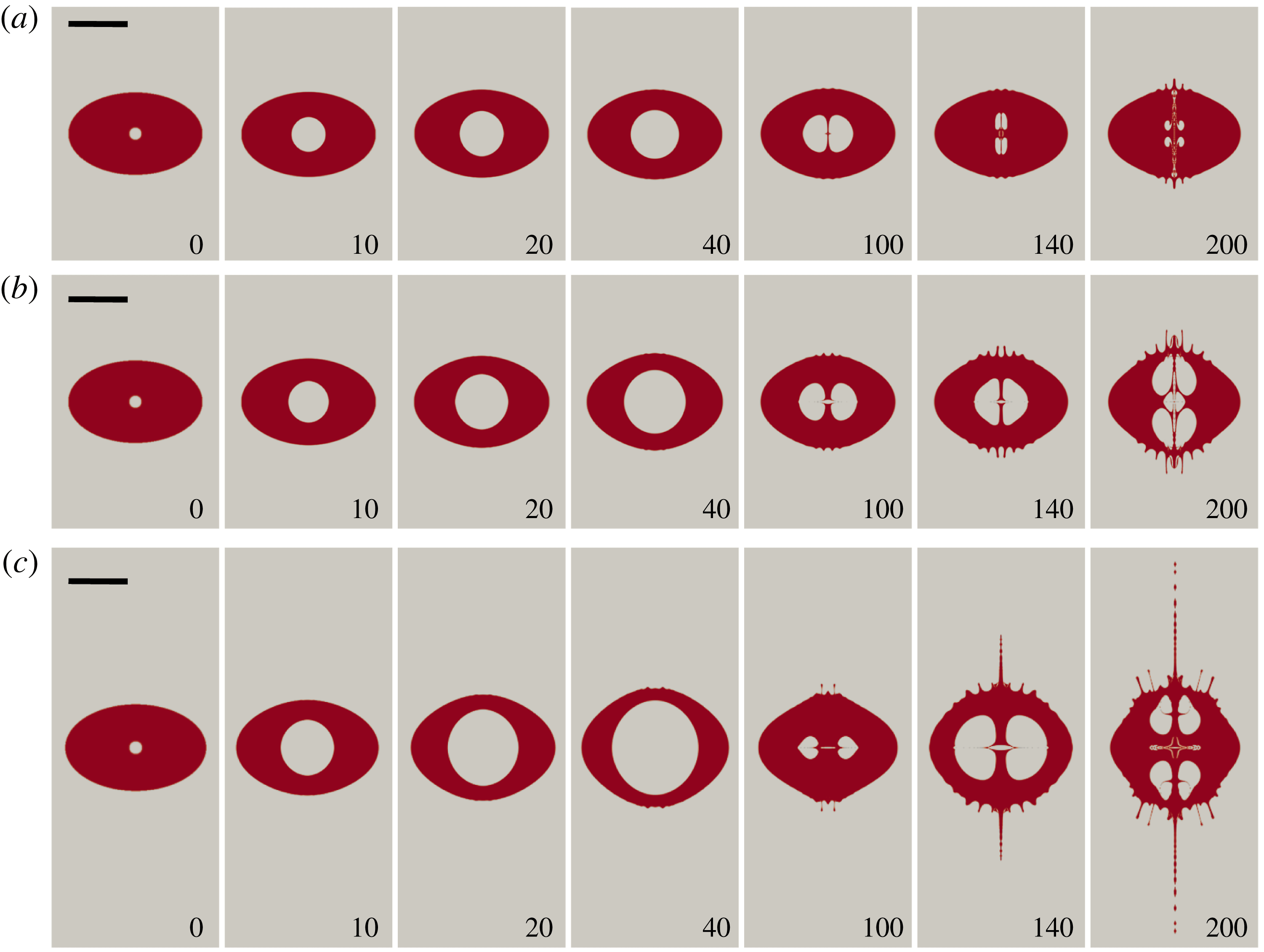
Comparison of 2-D axisymmetric simulation results under different initial internal pressure for 10 cSt oil droplet: (a) 50 bar; (b) 100 bar; (c) 250 bar. Time in
 $\unicode[STIX]{x03BC}\text{s}$
; the scale bar represents 1 mm;
 $R_{d,eq}=1.02~\text{mm}$
.

Comparison of 2-D axisymmetric simulation results under different viscosity and the same initial internal pressure 250 bar: (a) 10 cSt oil droplet; (b) 20 cSt oil droplet; (c) 50 cSt oil droplet. Time in
 $\unicode[STIX]{x03BC}\text{s}$
; the scale bar represents 1 mm;
 $R_{d,eq}=1.02~\text{mm}$
.

The initial acceleration of the droplet affects the amplitude and coverage of the surface ripples. Viscosity opposes the fluid acceleration and stabilizes the interface. Next we will compare axisymmetric simulations for different initial accelerations and viscosities to understand their effects on the jetting seen after the first bubble collapse. The initial acceleration is difficult to control experimentally and numerically, the simpler approach is to vary the initial potential energy of the bubble, accelerating the fluid and liquid–gas interface. Figure 8 summarizes results from three 2-D axisymmetric simulations with increasing bubble energy (from figure 8
a–c) while keeping the liquid properties and geometry constant, i.e. oil droplet at 10 cSt with initial bubble radius
 $R=100~\unicode[STIX]{x03BC}\text{m}$
. For an initial bubble pressure of 50 bar and 100 bar, only minute jets are seen after the first bubble collapse and these lengthen after the second collapse
 $t=200~\unicode[STIX]{x03BC}\text{s}$
. Most prominent is the increase in bubble volume with increasing pressure. For an initial pressure of 250 bar (figure 8
c), fast jets develop after the first bubble collapse. The surface instability modes and the position of the jets are similar for all the cases, yet the amplitudes of the perturbations increase with initial bubble energy.
Figure 9(a–c) illustrates axisymmetric simulations of the flows with increasing viscosity from top to bottom. Interestingly, although the bubble dynamics for these three cases is very similar, the jetting from the droplet is largely different; i.e. no jetting at
 $\unicode[STIX]{x1D707}=50~\text{cSt}$
while fast jets are seen at
 $\unicode[STIX]{x1D707}=20~\text{cSt}$
and
 $\unicode[STIX]{x1D707}=10~\text{cSt}$
. Fluid viscosity in this range affects the bubble dynamics only mildly yet it has a pronounced effect on the stability of the surface, particularly after the first bubble collapse.
Suppression of the jet formation of the bubble. (a) A 50 cSt oil droplet with initial pressure of 20 bar; the maximum bubble radius is approximately
 $330~\unicode[STIX]{x03BC}\text{m}$
. (b) A 500 cSt oil droplet with initial pressure of 250 bar; the maximum bubble radius is approximately
 $690~\unicode[STIX]{x03BC}\text{m}$
. Time in
 $\unicode[STIX]{x03BC}\text{s}$
; the scale bar represents 1 mm; droplet sizes are the same as in figure 9.

The internal cavitation bubble will move away from the nearest free surface due to the action of the secondary Bjerknes force. In a semi-infinite geometry the bubble translates away from the free surface and develops a jet in the direction of translation. Within a droplet two jets are formed from the locations closest to the free surface. The jets move towards the centre of the droplet and impact onto each other, re-directing the jet along the equatorial plane. The result of a bubble split into a torus with a liquid sheet in the equatorial plane is found in the simulations in figures 5 and 7–9. The strength of the jet is affected by viscosity and can be fully suppressed by viscosity. This is demonstrated in figure 10. Figure 10(a) presents the bubble dynamics in a 50 cSt oil droplet with an initial bubble pressure of 20 bar. The bubble expands and collapses spherically. In this case, the instability on the bubble surface is hindered by the viscosity. Figure 10(b) shows a bubble with a higher internal pressure of 250 bar. The development of jets within and on the surface of the droplet is hindered again with a viscosity of 500 cSt. The bubble expands and shrinks almost spherically, yet takes an ellipsoidal shape during collapse. While the viscosity suppresses jetting it does not guarantee a spherical shape during collapse.
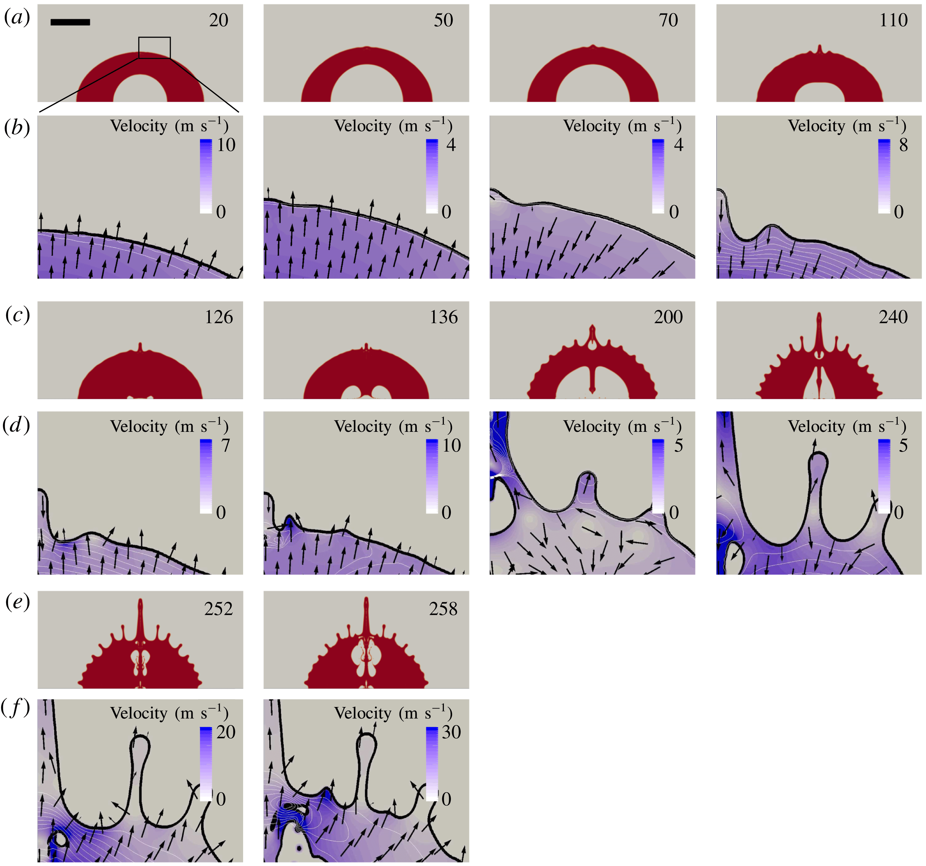
Flow details of a single water droplet near the surface at selected times. Time in
 $\unicode[STIX]{x03BC}\text{s}$
, and the scale bar represents 1 mm. (a,c,e) Overviews of the droplets’ surface shape, whose flow details in the black rectangle region are shown in (b,d,f). In (b,d,f), the black curve represents the surface, the white curve represents the contour line of pressure, the colour field is the contour face of velocity magnitude and the arrow represents the direction of velocity. Note that the colour fields are in a different range.

3.3 Mechanism of jetting
In this section we investigate the mechanism of the ejection of thin jets by analysing the velocity and pressure fields near the droplet’s outer surface. Figure 11 shows the surface evolution and the flow details of the water droplet from the axisymmetric simulation. We pay attention to how the velocity and pressure affect the shape of the droplet surface at later times. The droplet surface is smooth during the early expansion of the bubble (
 $t=20~\unicode[STIX]{x03BC}\text{s}$
) while the velocity and pressure are non-uniform along the surface, resulting in an undulating droplet later during bubble expansion, e.g. at
 $t=50~\unicode[STIX]{x03BC}\text{s}$
. During the shrinkage of the bubble (
 $t=70~\unicode[STIX]{x03BC}\text{s}$
), the liquid flows towards the droplet centre. The pressure field shows a wavy structure as it aligns to the surface corrugation. Troughs once formed on the surface are inherently unstable during the bubble collapse and extend in depth. This can be simply explained by the sink flow having a higher velocity for smaller
 $r$
which results in a growth of the amplitude of the surface perturbations during the bubble collapse (
 $t=110~\unicode[STIX]{x03BC}\text{s}$
). The bubble expands at
 $t=126~\unicode[STIX]{x03BC}\text{s}$
creating a pressure impulse. This accelerates the fluid surface such that troughs transform into crests (Antkowiak et al.
Reference Antkowiak, Bremond, Le Dizès and Villermaux2007) visible at
 $t=136~\unicode[STIX]{x03BC}\text{s}$
where jets form at the locations of previous troughs. The central retracting jet on the axis of symmetry is an exception: it merges with the newly created neighbouring jet and entraps a cavity (see figure 11,
 $t=200~\unicode[STIX]{x03BC}\text{s}$
). The velocities of the pressure-impulse-induced jets are considerably higher than the initial Rayleigh–Taylor instability created ones, leading to more filaments during the second bubble collapse at time
 $t=240~\unicode[STIX]{x03BC}\text{s}$
. This we explain with the fact that, between two jets, a new jet is formed from the troughs through the very same mechanism: see
 $t=258~\unicode[STIX]{x03BC}\text{s}$
.
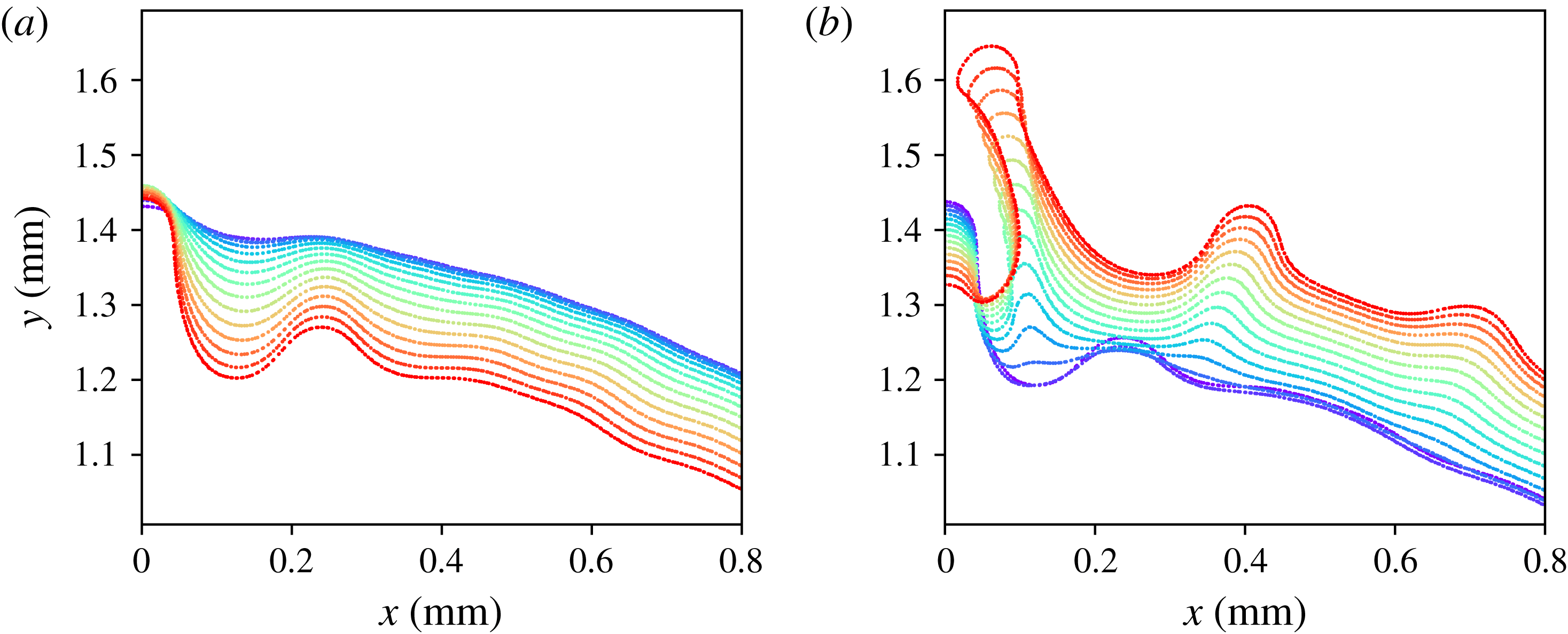
Zoomed view of the surface evolution of the water droplet during shrinkage (a) and expansion (b): (a)
 $t=60~\unicode[STIX]{x03BC}\text{s}$
to
 $t=118~\unicode[STIX]{x03BC}\text{s}$
; (b)
 $t=120~\unicode[STIX]{x03BC}\text{s}$
to
 $t=178~\unicode[STIX]{x03BC}\text{s}$
. Time increases from blue to red at intervals of
 $\unicode[STIX]{x0394}t=4~\unicode[STIX]{x03BC}\text{s}$
.

Let us now have a closer look at the shape of the droplet interface: figure 12 depicts the conversion of troughs into crests during the bubble collapse and expansion. Figure 12(a) covers the bubble shrinkage during the time
 $t=60~\unicode[STIX]{x03BC}\text{s}$
(top blue contour) until
 $t=118~\unicode[STIX]{x03BC}\text{s}$
(bottom red contour) spaced
 $\unicode[STIX]{x0394}t=4~\unicode[STIX]{x03BC}\text{s}$
in time. The surface disturbances are amplified during the bubble shrinkage. The bubble reaches minimum size at
 $t=124~\unicode[STIX]{x03BC}\text{s}$
which is covered in figure 12(b). Here the contours are staggered from the bottom (in blue,
 $t=120~\unicode[STIX]{x03BC}\text{s}$
) in time intervals of
 $\unicode[STIX]{x0394}t=4~\unicode[STIX]{x03BC}\text{s}$
to the top (red,
 $t=178~\unicode[STIX]{x03BC}\text{s}$
). The third contour
 $t=128~\unicode[STIX]{x03BC}\text{s}$
depicts the droplet shape just after re-expansion. At this time all troughs or concave features are flipped into crests or convex features. With time they develop into thin jets; the most pronounced is the jet closest to the axis of symmetry.
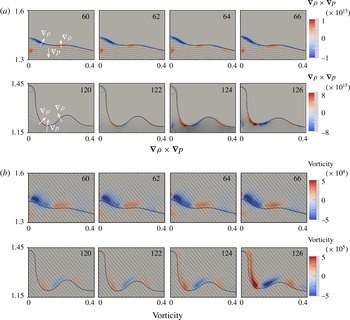
Flow details from the axisymmetric simulation. (a) The baroclinity; (b) the vorticity. Thick lines represent the surface, and thin lines are the pressure contours with a spacing of 2 kPa; the vector shows the flow direction. The colour fields show the component perpendicular to the slice plane: a positive value means outwards while a negative value means inwards. Time in
 $\unicode[STIX]{x03BC}\text{s}$
: from
 $t=60~\unicode[STIX]{x03BC}\text{s}$
to
 $t=66~\unicode[STIX]{x03BC}\text{s}$
is within the collapse of the bubble,
 $t=120~\unicode[STIX]{x03BC}\text{s}$
and
 $t=122~\unicode[STIX]{x03BC}\text{s}$
are the late stage of the bubble shrinkage,
 $t=124~\unicode[STIX]{x03BC}\text{s}$
and
 $t=126~\unicode[STIX]{x03BC}\text{s}$
are the re-expansion. The units of the axes are mm and the origin is the droplet centre.

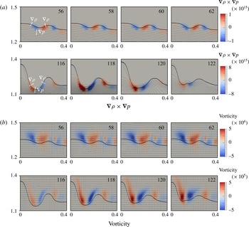
Flow details from the 3-D simulation. (a) The baroclinity; (b) the vorticity. Thick lines represent the surface, and thin lines are the pressure contours with a spacing of 2 kPa; the vector shows the flow direction. The colour fields show the component perpendicular to the slice plane: a positive value means outwards while a negative value means inwards. Time in
 $\unicode[STIX]{x03BC}\text{s}$
: from
 $t=56~\unicode[STIX]{x03BC}\text{s}$
to
 $t=62~\unicode[STIX]{x03BC}\text{s}$
is within the collapse of the bubble,
 $t=116~\unicode[STIX]{x03BC}\text{s}$
is the late stage of the bubble shrinkage, from
 $t=118~\unicode[STIX]{x03BC}\text{s}$
to
 $t=122~\unicode[STIX]{x03BC}\text{s}$
are the re-expansion. The units of the axes are mm and the origin is the droplet centre.

In general the Rayleigh–Taylor instability can be viewed as the result of baroclinity (Roberts & Jacobs Reference Roberts and Jacobs2016). It is proportional to
 $\unicode[STIX]{x1D735}\unicode[STIX]{x1D70C}\times \unicode[STIX]{x1D735}p$
, and thus formed by the misalignment of the density and the pressure gradients at the perturbed interface. Looking at the vorticity equation for compressible fluids
 $$\begin{eqnarray}\displaystyle \frac{\text{D}\unicode[STIX]{x1D74E}}{\text{D}t}=\frac{\unicode[STIX]{x2202}\unicode[STIX]{x1D74E}}{\unicode[STIX]{x2202}t}+(\boldsymbol{u}\boldsymbol{\cdot }\unicode[STIX]{x1D735}\unicode[STIX]{x1D74E})=\unicode[STIX]{x1D74E}\boldsymbol{\cdot }\unicode[STIX]{x1D735}\boldsymbol{u}-\unicode[STIX]{x1D74E}(\unicode[STIX]{x1D735}\boldsymbol{\cdot }\boldsymbol{u})+\frac{1}{\unicode[STIX]{x1D70C}^{2}}\unicode[STIX]{x1D735}\unicode[STIX]{x1D70C}\times \unicode[STIX]{x1D735}p, & & \displaystyle\end{eqnarray}$$
we see that baroclinity generates vorticity, feeding liquid into the jets. To document this mechanism we measure baroclinity and vorticity at the droplet surface and correlate them spatially and temporally with the formation of the troughs (during bubble shrinkage) and jets (during re-expansion) in axisymmetry (figure 13) and three dimensions (figure 14).
Figure 13 displays the evolution of baroclinity and vorticity from the axisymmetric simulation. The times
 $t=60~\unicode[STIX]{x03BC}\text{s}$
to
 $t=66~\unicode[STIX]{x03BC}\text{s}$
cover the early stage of bubble shrinkage, that is when the lighter fluid is accelerated into the heavier fluid. The pressure gradient in the direction towards the centre of the droplet and the density gradient are not parallel, resulting in a clockwise baroclinic torque on the surface created at the left side of the troughs and an anticlockwise baroclinic torque at the right side. The resulting vorticity amplifies the surface perturbation. At
 $t=120~\unicode[STIX]{x03BC}\text{s}$
, the late stage of the collapse, the direction of the pressure gradient is now away from the droplet centre. Thus the baroclinic torques change direction: anticlockwise at the left side and clockwise at the right side of the trough. Accordingly, the vorticity also changes direction, which results in a flipping of the troughs into crests. Because of the abrupt increase of the pressure gradient at the rebound
 $t=124~\unicode[STIX]{x03BC}\text{s}$
, a large increase in the vorticity at
 $t=126~\unicode[STIX]{x03BC}\text{s}$
is observed.
Figure 14 presents the dynamics of the baroclinity and vorticity from the 3-D simulation. They confirm that the mechanisms at work are the same as in the axisymmetric simulation. Please note the slightly different timing of the two simulations.
In summary, we can explain the pronounced jetting of low viscosity droplets with a two-step mechanism. First, the Rayleigh–Taylor instability prepares a corrugated surface on which the pressure impulse accelerates fine ligaments out of the troughs. Vorticity created through baroclinity feeds the ligaments. Later, during second bubble collapse, the flow field of the ligaments ‘detaches’ from the main droplet body and the ligaments do not retract but continue to move away. As a result, the droplet develops and partly disintegrates into the filamentary structure seen in the experiments, e.g. figure 1(a)
 $t=150~\unicode[STIX]{x03BC}\text{s}$
.
3.4 Stability analysis
Next we will discuss the stability of the droplet surface with the spherical droplet model derived in § 2.3. The parameters affecting jetting are bubble energy, droplet size, liquid viscosity, surface tension and the ambient pressure. We can formulate three dimensionless quantities, namely, normalized energy
 $E$
, Reynolds number
 $Re$
and Weber number
 $We$
:
 $$\begin{eqnarray}\displaystyle E & = & \displaystyle \frac{E_{b0}}{V_{d0}P_{\infty }}=\frac{V_{b0}P_{b0}}{V_{d0}P_{\infty }}=\frac{R_{b0}^{3}P_{b0}}{R_{d0}^{3}P_{\infty }},\end{eqnarray}$$
 $$\begin{eqnarray}\displaystyle Re & = & \displaystyle \frac{\unicode[STIX]{x1D70C}U_{ref}R_{d0}}{\unicode[STIX]{x1D707}},\end{eqnarray}$$
 $$\begin{eqnarray}\displaystyle \mathit{We} & = & \displaystyle \frac{\unicode[STIX]{x1D70C}U_{ref}^{2}R_{d0}}{\unicode[STIX]{x1D70E}},\end{eqnarray}$$
where
 $E_{b}$
is the initial bubble energy,
 $V$
is the volume,
 $R$
is the radius,
 $\unicode[STIX]{x1D70C}$
is the droplet density and the subscripts
 $b,d,0$
relate to the bubble, droplet and initial state, respectively. The reference velocity
 $U_{ref}=\sqrt{P_{\infty }/\unicode[STIX]{x1D70C}}$
is obtained from the closure time of a spherical void in an infinite medium.
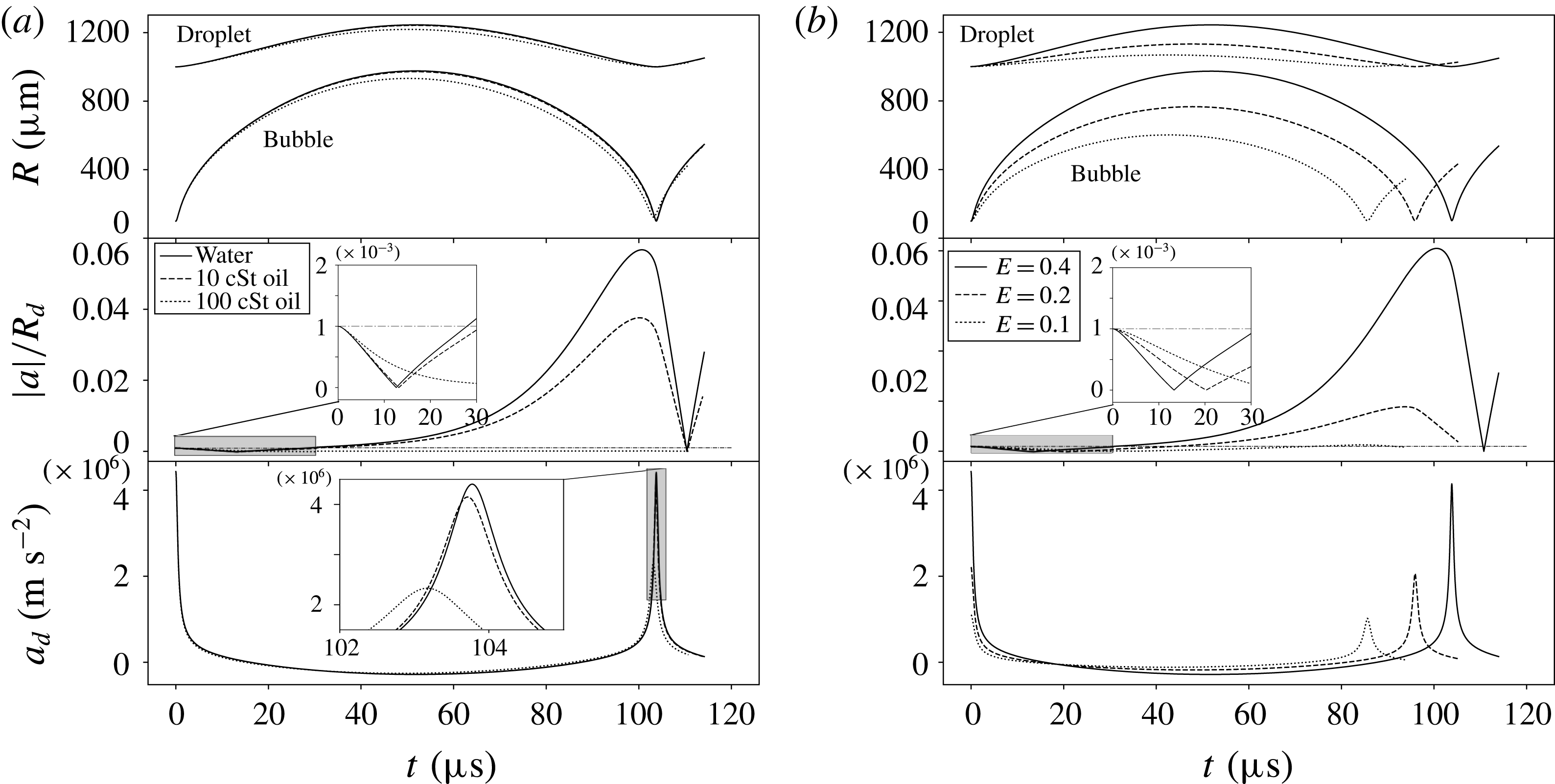
The radius and normalized perturbation amplitude. (a) Radius time traces (top), non-dimensional perturbation amplitude (middle) and the mean surface acceleration (bottom) of droplets with varying viscosity and constant normalized energy
 $E=0.4$
: for water
 $Re=10\,000$
, for 10 cSt oil
 $Re=1000$
, for 100 cSt oil
 $Re=100$
. (b) Comparison of droplets with different normalized energy but the same viscosity:
 $Re=1000$
, the normalized energies are
 $E=0.1$
, 0.2 and 0.4. The mode is 16 for all the cases in this figure. The dash-dot line is the initial perturbation.

The stability of the droplet surface is quantified by calculating the growth of an initial small yet finite surface perturbation. The results are only weakly affected by the particular choice of
 $a_{0}$
, which is here set to
 $a_{0}=0.001R_{d0}$
. Thus for a millimetre-sized droplet
 $a_{0}=1~\unicode[STIX]{x03BC}\text{m}$
. The amplitude of the surface perturbation is from now on stated by the non-dimensional disturbance
 $|a(t)|/R_{d}$
. Figure 15 depicts in the upper graphs the radius–time curve of the bubble and the droplet surfaces, in the middle graph the non-dimensional disturbance and in the lower graph the mean acceleration of the droplet surface. In figure 15(a) the viscosity is varied while the energy remains constant,
 $E=0.4$
, and in figure 15(b) the normalized energy is varied for a fixed dynamic viscosity of 10 cSt. We chose mode 16 for the disturbance: see later discussion.
Let us first look at the results for the water droplet in figure 15(a) (solid line) and the mode
 $n=16$
. The disturbance drops from 0.1% during the early expansion phase of the bubble (see inset) and then it grows 60-fold during the late expansion and early collapse to 6 %. During the late collapse and early rebound the disturbance on the droplet shrinks such that it returns back to its initial value around
 $t=110~\unicode[STIX]{x03BC}\text{s}$
. Naively, this would predict that the droplet surface is stabilized during the collapse and no jetting should be occurring. Yet, the incompressible model does not account for the acoustic wave emitted and its interaction with the surface. It is this wave that leads to the pressure impulse accelerating the droplet surface into thin jets. Thus, the important quantity to consider is the relative amplitude
 $|a(t=t_{c})|/R_{d}$
of the droplet surface at the time of bubble collapse,
 $t=t_{c}$
.
Let us now look at the effect of viscosity in figure 15(a) while keeping the initial energy constant. Viscosity affects the model through the normal stresses in the Rayleigh–Plesset equation (2.29) and the evolution equation for the disturbance (2.26). The first droplet/bubble oscillation cycle for a
 $\unicode[STIX]{x1D707}=10~\text{cSt}$
viscosity liquid is nearly indistinguishable from the water case, yet the amplitude at bubble collapse has markedly decreased to 4 % of the droplet radius. A ten-times higher viscosity
 $\unicode[STIX]{x1D707}=100~\text{cSt}$
, although it does mildly affect the bubble dynamics, fully prevents the growth of the instability. This is very similar to the observation in the experiment: see figure 3.
The second easily accessible parameter in the experiments is the internal energy of the bubble. Here, we fix the viscosity to 10 cSt and report three different energies
 $E$
in figure 15(b). In the upper graphs we see the expected effect that the bubble with larger energy expands to a larger maximum radius and therefore collapses later. Similarly, the amplitude of the disturbance as well as the mean acceleration of the droplet surface are largest for the highest energy. Yet, we find a clear threshold process: while the amplitude
 $|a(t=t_{c})|/R_{d}$
reaches 4 % for
 $E=0.4$
, it remains below and around 0.1 % for
 $E=0.1$
. This predicts that below a certain bubble/laser energy, the droplet will not result in jetting during the first collapse.
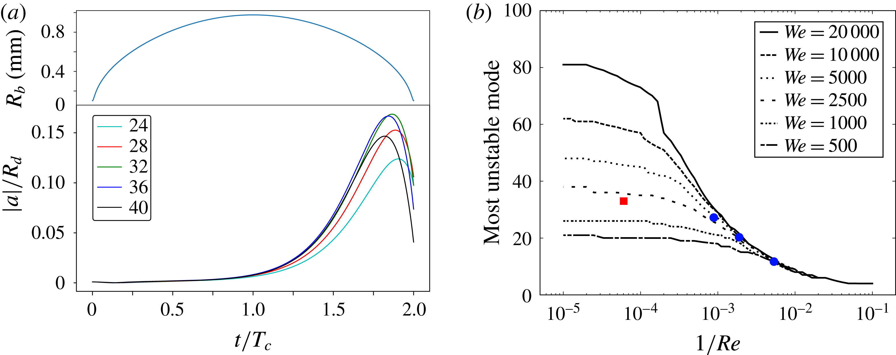
(a) The influence of the mode number
 $n$
on the perturbation growth for a water droplet of
 $Re=10\,000$
,
 $We=1428$
and
 $E=0.4$
. On top is the bubble radius time trace, on the bottom the normalized amplitude of the surface perturbations of the different mode numbers. The horizontal axis is the time normalized by the collapse time of the bubble
 $T_{c}$
. The most unstable mode is found between 24 and 32; (b) the most unstable mode versus
 $1/Re$
for different
 $We$
numbers. The red square represents the water droplet in figure 5, the bubble circles from left to right represent the oil droplets of 10, 20, 50 cSt viscosity in figure 9.

Finally, we discuss the effect of surface modes
 $n$
on the perturbation growth by studying the amplitudes of the surface mode n as a function of time: see (2.24). Once the parameters
 $Re$
,
 $We$
and
 $E$
are fixed, their growth is a function of the mode number
 $n$
only. For figure 16(a) we have chosen a specific triple of
 $Re=10,000$
,
 $We=1428$
and
 $E=0.4$
. We are specifically interested in the dominant mode at the collapse when the pressure impulse drives the jets from the troughs of the surface perturbations. A higher mode number would mean a larger number of jets paired with a smaller distance between neighbouring jets. The time in figure 16(a) is normalized by the Rayleigh collapse time
 $T_{c}$
of a bubble and droplet of the specific size. For the specific configuration we observe that the amplitude growth occurs during the early stage of the bubble collapse and is a strong function on the mode-
 $n$
. Here, an intermediate mode of
 $n=28$
has the highest amplitude at time
 $t=2T_{c}$
. Interestingly, the amplitudes of all modes shrink just before the bubble collapse and modes of highest amplitude over the whole cycle may not be dominant at the time of collapse, e.g. here
 $n=32$
versus
 $n=28$
.
Figure 16(b) reveals the dependency of the most unstable mode on the
 $Re$
and
 $We$
numbers, i.e. it is a combined effect of droplet size, surface tension and viscosity. The mode with the highest normalized amplitude at the minimum bubble radius is plotted in figure 16(b). For low viscosity or a small
 $1/Re$
number, the most unstable mode is approximately constant for a fixed
 $We$
number, thus it is then only a function of surface tension. The mode number
 $n$
decreases with higher surface tension. In the high
 $1/Re$
number regime, the viscous regime, the most unstable mode ceases to depend on the surface tension and viscosity dominates. The modes are considerably smaller than in the high
 $Re$
number regime.
Our experiments and simulations both show that with increasing viscosity the number of jets reduces and the droplet surface is smoother. This is in quantitative agreement with figure 16 (see also the cases in figure 16 b, symbols).
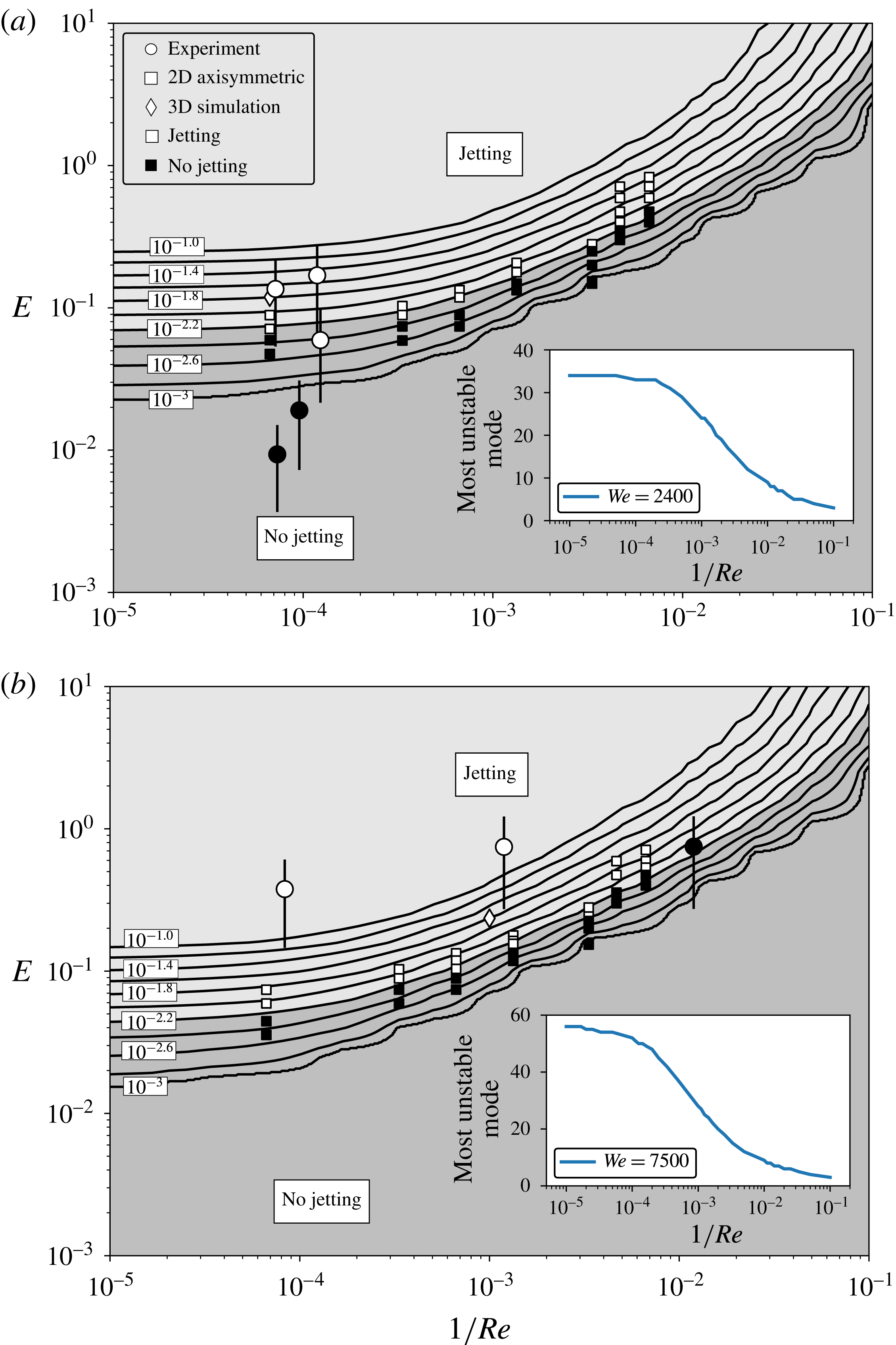
Jetting regimes. The parameter map consists of
 $1/Re$
on the horizontal axis and the normalized internal energy
 $E$
on the vertical axis. The contour represents the normalized amplitude of surface perturbations
 $|a|/R_{d}$
at the bubble collapse on a log scale. The circles represent experimental data; square symbols are 2-D axisymmetric simulation results; diamond symbols are 3-D simulation results. The filled symbols are the cases of jetting while the empty symbols are the cases of no jetting.

Next, we try to use the simple model for surface perturbations to predict the jetting regime. The axisymmetric, 3-D simulations, and the experiments are compared with the model. The underlying assumption is that jetting occurs once the surface perturbations are larger than some threshold needed for pressure-impulse-driven jetting.
Two parameter plots for the surface stability regimes are shown in figure 17 for
 $We=2400$
and
 $We=7500$
, respectively. Again, the inverse
 $Re$
-number is plotted on the horizontal and the normalized energy
 $E$
along the vertical axis. Filled symbols indicate non-jetting droplets, while open symbols are cases of jetting. Additionally, lines of constant normalized amplitude of the surface perturbation at minimum bubble volume are plotted. The value of
 $|a|/R_{d}$
is varied between 0.001 and 0.1 for 11 lines. We find that for
 $|a|/R_{d}\approx 0.63\,\%$
all but one measurement falls into the regime of jetting (above) or no jetting (below). Additionally, the most unstable mode is shown in the inset in figure 17 for the same inverse
 $Re$
-number regime as in the main plot.
The energy of the transition level is increasing from small
 $1/Re$
to large values. Thus, as expected, less energy is needed for low viscosity droplets to induce jetting. Interestingly, for not too large
 $1/Re$
, the energy remains approximately constant, indicating that surface tension and not viscosity is the limiting parameter stabilizing the droplet. For further increase, i.e. from
 $1/Re\approx 10^{-4}$
the energy grows approximately linearly in the double log plot in figure 17. A second parameter plot at a higher
 $We=7500$
is shown in figure 17(b) using the same values for the contours. The higher
 $We$
number leads to a lower energy threshold for jetting as compared to figure 17(a) for the low viscosity regime. The high viscosity regime reveals very similar boundaries for the normalized perturbation amplitude. Here again the threshold of
 $|a|/R_{d}=10^{-2.2}\approx 0.63\,\%$
seems to provide a good criterion between jetting and non-jetting.
In the experiments, the droplet due to the acoustic trapping does not obtain a spherical shape but is an oblate spheroid. In the stability analysis, however, we assumed a sphere and the results indicate that this is a reasonable approximation for not too large aspect ratio of the principal axes. In general, surface tension is a stabilizing force limiting the Rayleigh–Taylor instability (Trinh et al. Reference Trinh, Kim, Hammoud, Howell, Chapman and Stone2014), therefore one expects that the surfaces closer to the long axis of the oblate spheroid are more stable. Although this seems to be confirmed in the experiments, there the acceleration is also lower than at the upper and lower poles. A detailed evaluation of the effect of the shape of the droplet on the growth of the instability and jetting remains to be performed.
4 Conclusions
We have investigated a particular kind of jetting from single droplets caused by Rayleigh–Taylor instabilities in a spherical geometry. The instabilities lead to a corrugated liquid–air interface; upon collapse of the bubble, a pressure impulse focuses the troughs of the perturbed surface into thin jets. Most prominently, the number of jets decreases with viscosity. Experiments were reproduced with axisymmetric and 3-D CFD simulations. Good agreement of the bubble dynamics, the timing of jet formation and the location as well as the number of jets are found between experiments and simulations. Only the 3-D simulation reveals the cylindrical shape of the ejected jet, while the axisymmetric model would predict annular ring-shaped jets. An analytic model of the spherical Rayleigh–Taylor instability including viscosity based on Prosperetti’s (Prosperetti Reference Prosperetti1977) work has been re-derived.
The number of jets in the experiments and simulations is described well with the most unstable mode in the stability analysis. They depend only on
 $We$
-number and
 $Re$
-number. In the low
 $Re$
-number regime the droplet surface is mostly smooth with a small number of jets, while the high
 $Re$
-number regime displays many dimples resulting in more jets.
Although the analytic model is strictly valid only to first order in the perturbations and for incompressible flows, nevertheless, it is able to predict the onset of jetting as a function of
 $We$
number. This is shown by comparing the analytic model with simulation and experiments in the parameter map using
 $Re$
number and the normalized energy. The transition from jetting to non-jetting regimes seems to be close to
 $|a|/R_{d}=10^{-2.2}\approx 0.63\,\%$
. The minimum energy required for jetting increases approximately linearly in a double log plot of
 $1/Re$
versus
 $We$
. The jetting is dominated by
 $We$
number for low
 $1/Re$
number and independent of it at high
 $1/Re$
values.
The study has not explored the particular shape of the droplet. Although we have assumed for the analytic model that the droplet in the experiment is a sphere, an ellipsoidal shape may be more susceptible to the Rayleigh–Taylor instability as compared to a spherical droplet (Trinh et al. Reference Trinh, Kim, Hammoud, Howell, Chapman and Stone2014). It may be therefore interesting to extend the present study by utilizing the acoustic pressure to deliberately shape the bubble and to explore the importance of curvature on jetting.
The results may provide a pathway to explore flashing sprays. These are sprays consisting initially of large droplets governed by inertia. Before impact, the large droplets are activated by some physical or chemical mechanism resulting in a surface instability. The mechanism present in this study could help to design this process such that the droplets eject a suitable fine spray for a good surface coverage. We would also like to point out that this problem has some similarities to a branching firework with its resulting spectacular fragmentation dynamics (Inoue et al. Reference Inoue, Izato, Miyake and Villermaux2017).
Acknowledgement
We acknowledge anonymous referees for their very helpful suggestions to improve the manuscript.
Supplementary movies
Supplementary movies are available at https://doi.org/10.1017/jfm.2018.284.