I. INTRODUCTION
Size effect is the common term used to indicate the dependence of the stress–strain response on the specimen size. Size effects have been observed in torsion, Reference Fleck, Muller, Ashby and Hutchinson1–Reference Liu, He, Tang, Ding, Hu and Cao3 bending Reference Stölken and Evans4 experiments, and nanoindentation Reference Nix and Gao5 tests, while more recently they have been noted in the compression of micropillars. Reference Uchic, Dimiduk, Florando and Nix6,Reference Volkert and Lilleodden7 The most efficient framework for interpreting these effects is gradient plasticity, where gradients of the plastic strain are introduced into the constitutive equation of a plasticity framework. Over the past 30 years, numerous gradient plasticity formulations Reference Fleck, Muller, Ashby and Hutchinson1,Reference Aifantis8–Reference Voyiadjis and Faghihi17 have been established after Aifantis's initial proposal, Reference Aifantis8 and they are either phenomenologically or physically based. Fleck et al. Reference Fleck, Muller, Ashby and Hutchinson1 used the phenomenological strain gradient (SG) couple stress theory to explain the size effect observed in torsion experiments, and later reformulated and updated the theory, Reference Fleck and Hutchinson11,Reference Fleck and Willis13,Reference Fleck and Willis14 for instance, to accommodate the requirement of thermodynamic consistency. Reference Fleck and Hutchinson11 The so-called-mechanism-based SG theory was proposed by Nix, Gao, and Huang et al. Reference Nix and Gao5,Reference Gao, Huang, Nix and Hutchinson10 to explain a series of experiments related to size effects; a systematic exploration of size effects using the SG theory can also be found in Ref. Reference Aifantis18. Recently, a multilayer SG plasticity model has been used to model the strain burst or stress drop phenomena in micropillar compression. Reference Zhang and Aifantis19,Reference Konstantinidis, Aifantis and De Hosson20 A common feature of all these formulations is the prefactor of the SG, which for reasons of dimensional consistency must have the dimension of (an internal) length. The physical origin of the gradient term has already been discussed; Reference Aifantis21,Reference Zaiser and Aifantis22 however, the origin of this internal length scale has not yielded to a general physical interpretation. Reference Gurtin and Anand23 Many articles argue that the internal length scale in crystalline solids should be related to the dislocation microstructure of the material, Reference Gurtin and Anand23 invoking quantities such as the Burgers vector, Reference Gao and Huang24 the dislocation spacing, Reference Groma, Csikor and Zaiser25 or the dislocation source distance. Reference Aifantis and Ngan26 However, it is difficult to design experiments that provide quantitative information on dislocation processes on the scale of individual dislocations with good statistics.
The most effective way to capture dislocation interactions and the concomitant evolution of dislocation microstructures is through discrete dislocation dynamics (DDD) simulations. Reference Van der Giessen and Needleman27–Reference Weygand, Friedman, Van Der Giessen and Needleman29 Such simulations can also provide information on the plastic strain distribution on the dislocation scale. Relating, therefore, DDD simulations with gradient plasticity can help to interpret the internal length scale in terms of various dislocation characteristics. A first study performing such a comparison using 3D DDD was reported in Ref. Reference Aifantis, Senger, Weygand and Zaiser30 where strain distributions in simulated tricrystals were investigated. In that study it was concluded that the best agreement was obtained when the internal length scale had a value equal to the dislocation source distance. In those simulations, however, the dislocation source distance, dislocation source length, and dislocation spacing, had all approximately the same value, making it difficult to decide upon the relative importance of these parameters. It is more appropriate, therefore, to complement the simulations of Ref. Reference Aifantis, Senger, Weygand and Zaiser30 by systematically varying the relative magnitude of the length scale parameters which characterize the initial dislocation arrangement.
In the present article, 3D DDD simulations similar to those of Ref. Reference Weygand and Gumbsch31 were performed for tricrystals with a grain size of 750 nm, where the presence of grain boundaries (GBs) leads to SGs from the grain centers toward the boundaries. Three sets of simulations were performed, using initial dislocation source lengths of 100, 200, and 300 nm, while the other parameters of the initial dislocation microstructure (source spacing, number of sources per grain and slip system) were kept fixed for all the cases. From the DDD data, the dislocation density tensor was extracted, which in turn provided the plastic strain distribution throughout the specimen. Analytical expressions for the plastic strain profile, obtained from gradient plasticity, were then fitted to the expressions obtained from the simulations, leading to estimates for the internal length which allowed the study of the interdependence between the internal length scale and the dislocation source length.
In addition to using the internal length to account for the properties of internal boundaries, e.g., GBs, the framework of gradient plasticity has recently been extended to include another parameter which controls the interface strength and has the formal structure of an interface energy term. Reference Aifantis and Willis12 In analyzing the DDD simulations, two cases were considered for the GBs: they were either stiff and nondeforming or exhibited plastic yielding at finite strain. A best fit of gradient plasticity predictions to the DDD strain profiles in the latter case allowed us to obtain first estimates for the interface energy associated with GB yielding. Furthermore, by comparing the quality of fits obtained for both the cases we can assess whether the DDD data are better described in terms of stiff or deformable GBs.
II. DDD SIMULATIONS OF TRICRYSTAL PLASTICITY
DDD simulations were performed using aluminum samples that consisted of three cubic grains, each having a grain size of 750 nm. The loading axis lied on the [001] direction and all the grains were taken to share the same [001] axis, while the central grain was rotated by 22.5° around the loading axis with respect to the outer grains. The GBs were assumed to act as inert obstacles that were nonpenetrable by dislocations. Deformation was carried out at a strain rate of 5000/s.
The initial dislocation structure was constructed using Frank–Read sources of the same length. Each grain and each slip system contained the same number of sources, which were randomly oriented and randomly distributed over the available volume (conditional on the requirement that a source must not intersect a crystallite boundary). During plastic deformation these sources were activated and evolution of the dislocation network occurred. Dislocation motion is governed by the expression
 $$m\ddot x + \eta \dot x = f\quad ,$$
where m is the effective mass of dislocations per unit length and is taken to be 0.51 − 0.85 × 10¹⁶ kg/m, η is the drag coefficient (with a value of 10−4 Pa s), and f is the Peach–Koehler force acting on a dislocation segment.
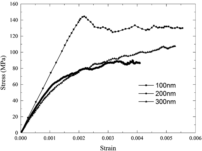
To investigate the effect of different internal length scales associated with the dislocation microstructure on the mechanical response of the tricrystal, simulations were carried out on samples with a dislocation source length of 100, 200, and 300 nm. The dislocation source spacing was kept at a constant value of 140 nm, leading to initial dislocation densities (ρ) of 3.75 × 10¹³ m−2, 7.5 × 10¹³ m−2, and 10.25 × 10¹³ m−2 and mean dislocation spacings (inverse square root of dislocation density) of 163, 115, and 99 nm, respectively. Stress–strain curves for the three cases are shown in Fig. 1. An effective elastic modulus E is obtained by computing the initial slope of the stress–strain curves, giving the values of E = 71, 60, and 53 GPa for source lengths of 100, 200, and 300 nm, respectively. This source length dependence can be understood by noting that dislocations start to bow out as soon as a stress (however small) is applied. This bowing out produces, in the initial deformation regime, a recoverable anelastic deformation which adds to the elastic strain and leads to a reduced effective modulus. Since it is easier for dislocations to bow out when dislocation sources are longer, the anelastic strain increases and as a consequence the effective elastic modulus of the tricrystals decreases.
Stress–strain curves obtained by DDD simulation of tricrystals with different source lengths.
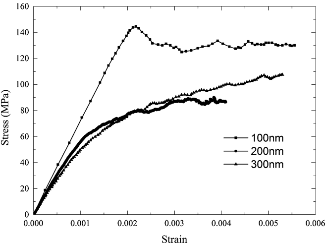
From the stress–strain curves, it is found that different dislocation source lengths also result in a different yield stress and strain hardening behavior. This can be readily understood if we note the different mechanisms which control the plastic flow in the three cases:
-
(i) For a source length of 100 nm, the source length is less than the initial mean dislocation spacing. In this case, the plastic flow is controlled by the self-interaction of the source segments, which governs the source activation, rather than by interactions between different segments. The activation stress τcr of a single dislocation source of length L FRS is determined as Reference Foreman32
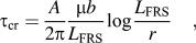 $${\tau _{{\rm{cr}}}} = {A \over {2\pi }}{{\mu b} \over {{L_{{\rm{FRS}}}}}}\log {{{L_{{\rm{FRS}}}}} \over r}\quad ,$$
where μ = 27 GPa is the shear modulus of aluminum, the value of A is determined by the dislocation source orientation (A equals 1 for edge dislocations, and 1/(1 − ν) for screw dislocations, where ν = 0.347 is the Poisson's ratio), and b = 0.286 nm is the length of the Burgers vector in aluminum. The quantity r is the cut-off length or Brown splitting distance, with a typical value of 2b. Reference Weygand, Friedman, Van Der Giessen and Needleman29
If yield is controlled by source activation, the activation stress
τcr can be related to the tensile yield stress
σcr by σcr =
τcr/(cosΦcosθ) where
cosΦcosθ is the Schmidt factor. In the DDD simulations, all the
grains share the same [100] axis, which is also the loading direction for the whole
tricrystal, such that eight slip systems with the same Schmidt factor of
 $\left( {{1 \mathord{\left/ {\vphantom {1 {\sqrt 2 }}} \right. \kern-\nulldelimiterspace} {\sqrt 2 }}} \right) \times \left( {{1 \mathord{\left/ {\vphantom {1 {\sqrt 3 }}} \right. \kern-\nulldelimiterspace} {\sqrt 3 }}} \right) \approx 0.408$
are potentially active. For a dislocation source length of 100 nm,
the activation stress for a source with edge orientation is about 140 MPa, which
agrees well with the yield point evident in Fig.
1 for the corresponding stress–strain curve. At higher strains,
dislocation–dislocation interactions may lead to the formation of larger
sources. As a result, we see little hardening, or indeed some softening, after
yield.
-
(ii) For a source length of 300 nm, the source length is much larger than the initial mean dislocation spacing. In this case, the sources strongly overlap and the plastic flow is controlled by interactions between segments from different sources. The yield stress can then be simply estimated using the Taylor relation,
 $${\tau _{{\rm{cr}}}} = \alpha \mu b\sqrt {\rho }\,\quad,$$
with a typical value of α = 0.3 this gives a yield stress of 57 MPa, again in good agreement with Fig. 1. After yield, the dislocation density increases and, unlike for the 100 nm case, significant strain hardening occurs.
-
(iii) The tricrystal with 200 nm source length is intermediate between the aforementioned cases – with respect to both the yield stress and the hardening coefficient. In this case, the respective contributions of dislocation–dislocation interactions and source activation to the overall flow stress are of comparable magnitude.
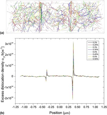
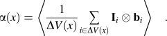
A most important feature of DDD simulations is that they provide the evolution of the dislocation structure. The geometrically necessary dislocation (GND) density tensor can be calculated, as a function of the position along the loading axis, as Reference Aifantis, Senger, Weygand and Zaiser30
 $$\alpha (x) = \left\langle {{1 \over {\Delta V(x)}}\mathop\sum\limits_{i \in \Delta V(x)} {{{\rm \bf I}_i} \otimes {{\rm \bf b}_i}} } \right\rangle \quad .$$
Here ΔV(x) is a slice of the specimen, perpendicular to the loading axis, which is centered at position x along the loading direction. The sum runs over all dislocation segments i intersecting this slice, l i is the vector which connects the two nodal points delimiting a segment (if only part of the segment is contained in ΔV(x), l i is the vector which connects the entry point with the nodal point inside ΔV(x)), and b i is the Burgers vector of the segment. The symbol <> means that the calculation is averaged over multiple simulations and also over symmetry equivalent positions within the simulated samples. The simulated samples are divided into 120 slices and the thickness of each slice is 18.75 nm for the tricrystal with 100 or 300 nm source length, while tricrystals with 200 nm source length are divided into 30 slices of 75 nm thickness. During the deformation, the dislocation distribution and the corresponding GND profile evolve as shown in Fig. 2.
(a) Dislocation structure of a simulated tricrystal at a total strain of 0.26%. (b) Distribution and evolution of the dislocation density tensor component α32 during deformation of a single tricrystal specimen (dislocation source length 100 nm) from 0.2 to 0.55% total strain, averaged over slices perpendicular to the loading axis, plotted versus position along the loading axis.

The plastic strain profiles can then be determined through the following relationship between the SG and the GND density Reference Fleck, Muller, Ashby and Hutchinson1 :
 $$\alpha _{{\rm{in}}} = e_{nkj} \gamma _{ij,k} \quad ,$$
where αin is the Kröner–Nye
tensor and
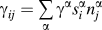 $\gamma _{ij} = \mathop\sum\limits_\alpha {\gamma ^\alpha s_i^\alpha n_j^\alpha }$
is the plastic distortion tensor with
 $s_i^\alpha$
and
 $n_j^\alpha$
to be the slip direction and slip plane normal of α slip
system. Equation (5) can further be
written in a component form as follows:
 $$\left[ {\matrix{ {\alpha _{11} } & {\alpha _{12} } & {\alpha _{13} } \cr {\alpha _{21} } & {\alpha _{22} } & {\alpha _{23} } \cr {\alpha _{31} } & {\alpha _{32} } & {\alpha _{33} } \cr } } \right] = \left[ {\matrix{ {\gamma _{13,2} - \gamma _{12,3} } & {\gamma _{11,3} - \gamma _{13,1} } & {\gamma _{12,1} - \gamma _{11,2} } \cr {\gamma _{23,2} - \gamma _{22,3} } & {\gamma _{21,3} - \gamma _{23,1} } & {\gamma _{22,1} - \gamma _{21,2} } \cr {\gamma _{33,2} - \gamma _{32,3} } & {\gamma _{31,3} - \gamma _{33,1} } & {\gamma _{32,1} - \gamma _{31,2} } \cr } } \right]\quad .$$
It should be noted that upon averaging over a slice perpendicular to the tensile axis the shear components of the plastic distortion tensor vanish during tensile deformation, and the same holds true for the gradients along the lateral direction. Thus, the relationship between the GND and plastic distortion tensors is given by
 $$\left[ {\matrix{ {\alpha _{11} } & {\alpha _{12} } & {\alpha _{13} } \cr {\alpha _{21} } & {\alpha _{22} } & {\alpha _{23} } \cr {\alpha _{31} } & {\alpha _{32} } & {\alpha _{33} } \cr } } \right] = \left[ {\matrix{ 0 & 0 & 0 \cr 0 & 0 & {\gamma _{22,1} } \cr 0 & { - \gamma _{33,1} } & 0 \cr } } \right]\quad .$$
The plastic distortion tensor is related to the plastic strain tensor through the
relationship
 $\varepsilon _{ij}^{\rm{p}} = {{\left( {\gamma _{ij} + \gamma _{ji} } \right)} \mathord{\left/ {\vphantom {{\left( {\gamma _{ij} + \gamma _{ji} } \right)} 2}} \right. \kern-\nulldelimiterspace} 2}$
, and thus
 $\varepsilon _{11}^{\rm{p}} = {\gamma _{11}},\;\varepsilon _{22}^{\rm{p}} = {\gamma _{22}},\;\varepsilon _{33}^{\rm{p}} = {\gamma _{33}}$
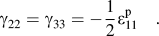
. It is also noted that because of plastic incompressibility
 $\varepsilon _{11}^{\rm{p}} + \varepsilon _{22}^{\rm{p}} + \varepsilon _{33}^{\rm{p}} = 0$
, so
 $${\gamma _{22}} = {\gamma _{33}} = - {1 \over 2}\varepsilon _{11}^{\rm{p}}\quad .$$
Substitution of (8) into (7) yields the following relationship between the GND tensor and plastic strain tensors.
 $$\left[ {\matrix{ {\alpha _{11} } & {\alpha _{12} } & {\alpha _{13} } \cr {\alpha _{21} } & {\alpha _{22} } & {\alpha _{23} } \cr {\alpha _{31} } & {\alpha _{32} } & {\alpha _{33} } \cr } } \right] = \left[ {\matrix{ 0 & 0 & 0 \cr 0 & 0 & { - {1 \over 2}\varepsilon _{11,1}^{\rm{p}} } \cr 0 & {{1 \over 2}\varepsilon _{11,1}^{\rm{p}} } & 0 \cr } } \right]\quad .$$
It follows that α23 and α32 are the two
important GND components which are used to obtain the plastic strain profile. Figure 2(b) depicts the resulting distribution
and evolution of the GND density component α32 during the
tensile deformation until a total strain level of 0.55% for tricrystals with
dislocation source length of 100 nm. The corresponding profile of the plastic strain
component
 $\varepsilon _{11}^{\rm{p}}$
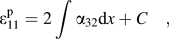
is then evaluated by integration either as
 $$\varepsilon _{11}^{\rm{p}} = 2\int {\alpha _{32} {\rm{d}}x} + C\quad ,$$
or
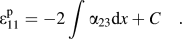 $$\varepsilon _{11}^{\rm{p}} = - 2\int {\alpha _{23} {\rm{d}}x} + C\quad .$$
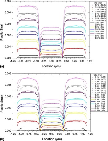
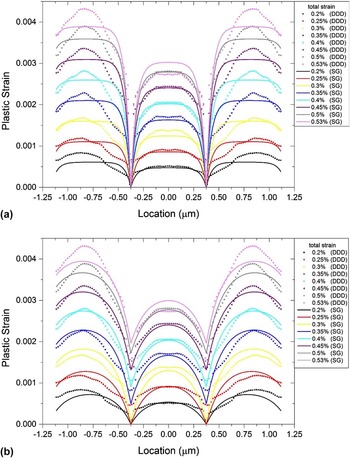
Plastic strain profiles for tricrystals at different total strains with a dislocation source length of 100 nm, profile data determined from DDD and SG plasticity fits; (a) rigid GBs and (b) strain profiles after coarse graining with SG fits assuming GBs of finite strength.

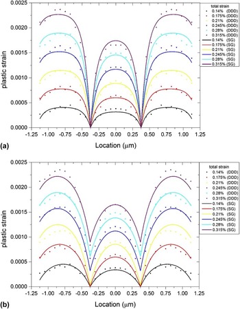
In our work, we average the plastic strains obtained from Eqs. (10) and (11) such as to reduce the statistical error. The integration constants in Eqs. (10) and (11) are determined by imposing the plastic strain at the GBs (which are impenetrable to dislocations) to be zero. Figures 3(a)–Figures 5(a) show the plastic strain profiles for tricrystals with dislocation source lengths of 100, 200, and 300 nm which have been determined in this manner. In the following text, we use these profiles for comparing with the results of gradient plasticity calculations for the case of impenetrable GBs.
Plastic strain profiles for tricrystals at different total strains with a dislocation source length of 200 nm, profile data determined from DDD and SG plasticity fits; (a) rigid GBs and (b) strain profiles after coarse graining with SG fits assuming GBs of finite strength.

Plastic strain profiles for tricrystals at different total strains with a dislocation source length of 300 nm, profile data determined from DDD and SG plasticity fits; (a) rigid GBs and (b) strain profiles after coarse graining with SG fits assuming GBs of finite strength.

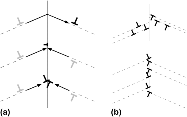
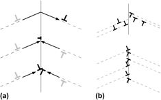
In our DDD simulations, the GBs are nonpenetrable to dislocations which therefore are deposited on both their sides. However, when we analyze the data in terms of the continuum gradient plasticity, we consider the evolution of strain fields on scales above the single-dislocation level and on these scales it is not a foregone conclusion that GBs do not yield, even if they are physically impenetrable to dislocations. This seemingly paradoxical statement can be readily understood by noting that, on the continuum scale, the transmission of a dislocation through a GB and the deposition of two dislocations in the GB may produce exactly the same plastic strain [Fig. 6(a)]. Also, on the continuum scale we cannot distinguish between two dislocations that are absorbed into the GB (losing their individuality due to atomic rearrangements) and two dislocations that are deposited on both sides of the GB while keeping their individuality. All these processes lead to the same plastic strain field and must therefore, on the continuum scale, be envisaged in common terms, i.e., as GB yielding. On the other hand, the formation of a dislocation boundary layer which extends over a distance above the dislocation spacing into the bulk and leads to a SG over the same length scale must be considered the equivalent of a nonyielding GB on the continuum scale [Fig. 6(b)].
(a) Three dislocation processes all of which produce the same strain field: Dislocation transmission at GB, absorption of two dislocations into GB, and storage of two dislocations on both sides of the GB; (b) top: a GB which is not yielding on the scale of a continuum description and bottom: a GB which on the continuum scale exhibits GB yielding.
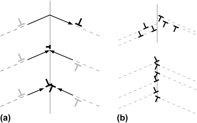
The question is thus whether dislocations “condense” on the GB [yielding, lower part of Fig. 6(b)] or distribute over an extended boundary layer [no GB yielding, upper part of Fig. 6(b)]. In our analysis, we distinguish these two cases by coarse graining the SG and relaxing the requirement that the strain at the GB be zero. If the GB does not yield, i.e., if there is an extended plastic boundary layer on both sides, this operation will not change the strain field to an appreciable extent. If, on the other hand, most dislocations are deposited directly at the boundary then the associated gradients will partly cancel upon coarse graining and the coarse-grained strain field will then be nonzero at the GB. The plastic strain profiles after coarse graining are shown in Figs. 3(b)–Figs. 5(b).
For relating the DDD data with gradient plasticity results, we compare the profiles of Figs. 3–5 with the results calculated for GBs of infinite and finite strength, using in the latter case the GB strength parameter as an additional fit parameter in the models. Comparing the quality of fits obtained under both assumptions allows us to decide which viewpoint yields a better continuum description of the DDD data.
III. THE SG FRAMEWORK FOR A TRICRYSTAL
SG models have been successfully used to describe the mechanical behavior of materials undergoing heterogeneous deformation on the continuum scale. Interfaces and surfaces are common sources for the development of heterogeneous deformation due to the associated constraints on dislocation movement. In a tricrystal, the rigid interface and the free surface affect the dislocation evolution and the resulting plastic deformation dramatically. Here we investigate the extent to which a SG plasticity model can reproduce the resulting strain heterogeneities in a continuum framework.
Since the tricrystal at hand had two GBs it is important to explicitly account for
their presence. The gradient plasticity framework employed, hence, is that proposed
in Ref. 12 in which a separate interface energy that depends on the plastic strain
at the interface was introduced. This model has been shown to be in good agreement
with experimental evidence regarding interface–GB interactions during nanoindentation,
Reference Aifantis and Ngan26
and it has been possible to successfully interpret the inverse
Hall–Petch relationship observed for nanocrystals.
Reference Aifantis and Konstantinidis33,Reference Zhang and Aifantis34
It is, therefore, important to physically understand the origin
of the two parameters that come into play in such an interface gradient plasticity
model, which are the internal length scale and a newly introduced interface
parameter. This can be done by directly relating the theoretically predicted
stress–strain curves to the DDD data. Before doing so, a brief
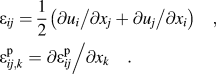
description of the model is given. Within a SG framework, the displacement vector
with components u
i
and plastic strain tensor with components
 $\varepsilon _{ij}^{\rm{p}}$
are treated as independent variables, and are assumed to be
continuous across the whole material. Other kinetic variables like total strain and
plastic SG can be expressed through u
i
and
 $\varepsilon _{ij}^{\rm{p}}$
as
 $$\eqalign{ & {\varepsilon _{ij}} = {1 \over 2}\left( {{{\partial {u_i}} \mathord{\left/ {\vphantom {{\partial {u_i}} {\partial {x_j}}}} \right. \kern-\nulldelimiterspace} {\partial {x_j}}} + {{\partial {u_j}} \mathord{\left/ {\vphantom {{\partial {u_j}} {\partial {x_i}}}} \right. \kern-\nulldelimiterspace} {\partial {x_i}}}} \right)\quad , \cr & \varepsilon _{ij,k}^{\rm{p}} = {{\partial \varepsilon _{ij}^{\rm{p}}} \mathord{\left/ {\vphantom {{\partial \varepsilon _{ij}^{\rm{p}}} {\partial {x_k}}}} \right. \kern-\nulldelimiterspace} {\partial {x_k}}}\quad . \cr}$$
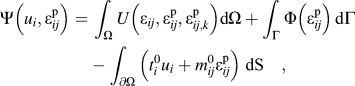
We consider the potential “energy” functional of the tricrystal,
 $$\Psi \left( {{u_i},\varepsilon _{ij}^{\rm{p}}} \right) =\, \int_\Omega {U\left( {{\varepsilon _{ij}},\varepsilon _{ij}^{\rm{p}},\varepsilon _{ij,k}^{\rm{p}}} \right)} {\rm{d}}\Omega + \int_\Gamma {\Phi \left( {\varepsilon _{ij}^{\rm{p}}} \right)} \,{\rm{d}}\Gamma - \int_{\partial \Omega } {\left( {t_i^0{u_i} + m_{ij}^0\varepsilon _{ij}^{\rm{p}}} \right)\;{\rm{dS}}\quad {\rm{,}}}$$
which consists of the elastoplastic energy U in the
volume Ω, external work on the outer surface ∂Ω, and
the interface energy Φ across the interface Γ. The main feature
of the above definition is that, in addition to the work of the tractions
 $t_i^0$
, the work done by hypertractions
 $m_{ij}^0$
on the plastic strain on the outer surface is considered, and that
the SG enters into the definition of the elastoplastic energy U
which has the form
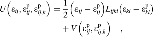 $$U\left( {{\varepsilon _{ij}},\varepsilon _{ij}^{\rm{p}},\varepsilon _{ij,k}^{\rm{p}}} \right) =\, {1 \over 2}\left( {{\varepsilon _{ij}} - \varepsilon _{ij}^{\rm{p}}} \right){L_{ijkl}}\left( {{\varepsilon _{kl}} - \varepsilon _{kl}^{\rm{p}}} \right) + V\left( {\varepsilon _{ij}^{\rm{p}},\varepsilon _{ij,k}^{\rm{p}}} \right)\quad ,$$
where L
ijkl
is the elastic stiffness tensor, ε
ij
is the total strain,
 $\varepsilon _{ij}^{\rm{p}}$
the plastic strain, and
 $\varepsilon _{ij,k}^{\rm{p}}$
is the plastic SG. The first term of Eq. (14) represents the elastic energy and the second term
represents the plastic energy, which includes energy contributions associated with
the presence of plastic SGs.
The Cauchy stress, back stress, and higher-order stress (or hyperstress) are conjugates to the elastic strain, plastic strain, and plastic SG, respectively:
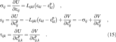 $$\hskip0.5pt\eqalignno{ & {\sigma _{ij}} = {{\partial U} \over {\partial {\varepsilon _{ij}}}} = {L_{ijkl}}\left( {{\varepsilon _{kl}} - \varepsilon _{kl}^{\rm{p}}} \right)\quad , \cr & {s_{ij}} = {{\partial U} \over {\partial \varepsilon _{ij}^{\rm{p}}}} = - {L_{ijkl}}\left( {{\varepsilon _{kl}} - \varepsilon _{kl}^{\rm{p}}} \right) + {{\partial V} \over {\partial \varepsilon _{ij}^{\rm{p}}}} = - {\sigma _{ij}} + {{\partial V} \over {\partial \varepsilon _{ij}^{\rm{p}}}}\quad , \cr & {\tau _{ijk}} = {{\partial U} \over {\partial \varepsilon _{ij,k}^{\rm{p}}}} = {{\partial V} \over {\partial \varepsilon _{ij,k}^{\rm{p}}}}\quad . \llab\hskip9.8pc(15)}\cr\}$$
Then taking the first variation of Ψ equal to zero gives the equilibrium equations
 $${\sigma _{ij,\,j}} = 0\;\;{\rm{in}}\;\Omega \quad ,$$
 $${s_{ij}} = {\tau _{ijk,k}}\;\;{\rm{in}}\;{\rm{ }}\Omega \quad ,$$
as well as the boundary condition
 $$\sigma _{ij} n_j = t_i^0 \;\;{\rm{on}}\;\partial \Omega \quad ,$$
 $$\tau _{ijk} n_k = m_{ij}^0 \;\;{\rm{on}}\;\partial \Omega \quad ,$$
along with the interface conditions
 $$\left[ {{\sigma _{ij}}{n_j}} \right] = 0\quad ,$$
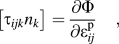 $$\left[ {{\tau _{ijk}}{n_k}} \right] = {{\partial \Phi } \over {\partial \varepsilon _{ij}^{\rm{p}}}}\quad ,$$
where [ ] denotes the jump of the pertinent variables across the interface or GB.
To proceed further, assumptions on constitutive equations for the plastic potential
and the interface energy are required. We consider a one-dimensional (1D) problem
where the deformation state is completely characterized by the axial strain
ε which depends on the axial position x only. The central
grain is located in the interval −L/2 <
x < L/2 and the outer grains in the
intervals
 ${L \mathord{\left/ {\vphantom {L 2}} \right. \kern-\nulldelimiterspace} 2} \lt \left| x \right| \lt {{3L} \mathord{\left/ {\vphantom {{3L} 2}} \right. \kern-\nulldelimiterspace} 2}$
. The GBs are located at x =
±L/2, and the specimen end surfaces at
x = ±3L/2. The plastic energy
for the middle grain and the adjacent surface grains is defined by
 $${V_i}\left( {{\varepsilon ^{\rm{p}}},\varepsilon _{,x}^{\rm{p}}} \right) = {\sigma _0}\left| {{\varepsilon ^{\rm{p}}}} \right| + {1 \over 2}{\beta _i}{\left( {{\varepsilon ^{\rm{p}}}} \right)^2} + {1 \over 2}{\beta _i}{\ell ^2}{\left( {\varepsilon _{,x}^{\rm{p}}} \right)^2}\quad ,$$
where the subscript i = m, s distinguishes the middle grain and surface grains. The first term in Eq. (22) suggests that the grain begins to deform plastically when the applied stress reaches a yield stress σ0. The second quadratic term describes a linear strain hardening, while the last quadratic term represents a SG hardening effect. The parameter ℓ is the internal length scale, which is required in the gradient term for dimensional consistency. In physical terms, this parameter needs to be related to length scales characterizing the microstructure of the material such as dislocation source length, dislocation spacing, or another dominant characteristic of the underlying deformation configuration. Note that, since the initial dislocation microstructure is statistically equivalent in all the three grains, we assume a common yield stress and length scale parameter. Hardening, however, is influenced by the boundary conditions which are different for the central and outer grains, which is why we allow for different hardening coefficients βm and βs.
The interfacial energy term is assumed as in, Reference Aifantis and Willis12
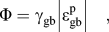 $$\Phi = {\gamma _{{\rm{gb}}}}\left| {\varepsilon _{{\rm{gb}}}^{\rm{p}}} \right|\quad ,$$
where γgb is a parameter with the dimensions of
an interface energy which controls the plastic yielding of the GB and
 $\varepsilon _{{\rm{gb}}}^{\rm{p}}$
is the plastic strain at the interface. In addition to the GB, we
also characterize the left and right end surfaces of the specimen by a finite
strength parameter γsf. This parameter accounts for the
repulsion of dislocations at the end surfaces where displacement boundary conditions
are applied in the finite element method used in the DDD. The effective repulsion
depends on the finite element resolution. These surfaces have therefore also in the
DDD problem a finite strength for blocking dislocations. In the strain profiles
(Figs. 3–5) this effect can be seen as a decrease of the plastic strain
toward the specimen ends.
Upon substitution of Eq. (22) into Eq. (15), the field Eqs. (16) and (17) give the differential equations for the displacement and plastic strain as follows:
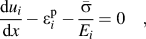 $${{{\rm{d}}u_i } \over {{\rm{d}}x}} - \varepsilon _i^{\rm{p}} - {{\bar \sigma } \over {E_i }} = 0\quad ,$$
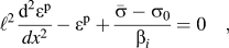 $$\ell ^2 {{{\rm{d}}^2 \varepsilon ^{\rm{p}} } \over {dx^2 }} - \varepsilon ^{\rm{p}} + {{\bar \sigma - \sigma _0 } \over {\beta _i }} = 0\quad ,$$
where the hardening coefficient β
i
may be different in the middle (i = m) and surface
(i = s) grains and
 $\bar \sigma$
is the homogeneous stress in 1D tension. To solve the above
equations, boundary conditions and interfacial conditions are required. For the
considered 1D geometry, the higher-order stress is
 $\tau = \beta {\ell ^2}\varepsilon _{,x}^{\rm{p}}$
. Substitution of Eq.
(23) into Eq. (21) then
gives the interface condition
 $${\gamma _{{\rm{gb}}}} \,\ge \pm {\ell ^2}\left( {{\beta _{\rm{s}}}{{\left. {{{\partial \varepsilon _{\rm{s}}^{\rm{p}}} \over {\partial x}}} \right|}_{ \pm L/2}} - {\beta _{\rm{m}}}{{\left. {{{\partial \varepsilon _{\rm{m}}^{\rm{p}}} \over {\partial x}}} \right|}_{ \pm L/2}}} \right)\quad ,$$
where the “>” holds prior to GB
yielding
 $\left( {\varepsilon _{{\rm{gb}}}^{\rm{p}}} \right) = 0$
and the equality “=” holds after GB
yielding
 $\left( {\varepsilon _{{\rm{gb}}}^{\rm{p}} > 0} \right)$
. In addition, we have in the latter case the standard requirement
of continuity of strain across the GB. At the end surfaces the corresponding
condition reads
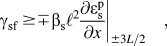 $${\gamma _{{\rm{sf}}}} \,\ge \mp {\beta _{\rm{s}}}{\ell ^2}{\left. {{{\partial \varepsilon _{\rm{s}}^{\rm{p}}} \over {\partial x}}} \right|_{ \pm 3L/2}}\quad ,$$
where again the “>” holds prior to end
surface yielding
 $\left( {\varepsilon _{\rm{s}}^{\rm{p}} = 0} \right)$
and the equality “=” holds after GB
yielding
 $\left( {\varepsilon _{\rm{s}}^{\rm{p}} > 0} \right)$
.
For a given set of parameters {P} = {σ0, ℓ, βm, βs, γsf, γgb} we can in general distinguish three regimes: (i) for σ0 < σ ≤ σ1, the grain interiors deform plastically but neither the GB nor the end surfaces have yielded, (ii) for σ1 < σ ≤ σ2, the end surfaces have yielded but the GB has not, and (iii) for σ > σ2, both the GB and the end surfaces have yielded. (The fourth possibility, namely that the GB yields but the end surfaces do not, is discarded. In this case the strain at the GB would be larger than the strain at the end surfaces, which is at variance with the DDD strain profiles, see Figs. 3–5.)
We first study case (i). In this case the strain is zero both at the GBs and at the end surfaces, and the strain profile is given by
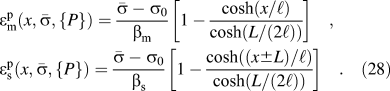 $$\hskip0.5pt\eqalignno{ & \varepsilon _{\rm{m}}^{\rm{p}}\left( {x,\bar \sigma ,\{ P\} } \right) = {{\bar \sigma - {\sigma _0}} \over {{\beta _{\rm{m}}}}}\left[ {1 - {{\cosh \left( {{x \mathord{\left/ {\vphantom {x \ell }} \right. \kern-\nulldelimiterspace} \ell }} \right)} \over {\cosh \left( {{L \mathord{\left/ {\vphantom {L {\left( {2\ell } \right)}}} \right. \kern-\nulldelimiterspace} {\left( {2\ell } \right)}}} \right)}}} \right]\quad, \cr & \varepsilon _{\rm{s}}^{\rm{p}}\left( {x,\bar \sigma ,\{ P\} } \right) = {{\bar \sigma - {\sigma _0}} \over {{\beta _{\rm{s}}}}}\left[ {1 - {{\cosh \left( {{{\left( {x \pm L} \right)} \mathord{\left/ {\vphantom {{\left( {x \pm L} \right)} \ell }} \right. \kern-\nulldelimiterspace} \ell }} \right)} \over {\cosh \left( {{L \mathord{\left/ {\vphantom {L {\left( {2\ell } \right)}}} \right. \kern-\nulldelimiterspace} {\left( {2\ell } \right)}}} \right)}}} \right]\quad .\hskip9.8pt(28)\cr}$$
With increasing stress, the SG at the outer surface increases. At the critical stress value
 $${\sigma _1} = {\sigma _0} + {{{\gamma _{{\rm{sf}}}}} \over {\ell \tanh \left( {{L \mathord{\left/ {\vphantom {L {\left( {2\ell } \right)}}} \right. \kern-\nulldelimiterspace} {\left( {2\ell } \right)}}} \right)}}\quad ,$$
it exceeds the critical value defined by the inequality (27), and the end surfaces yield. The
solution at this stress is denoted by
 $\varepsilon _{{\rm{m,s}}}^{\rm{p}}\left( {x,{\sigma _{\rm{1}}},\{ P\} } \right)$
. In regime (ii), the solution in the central grain is still given
by the expression (27); however,
the strain profile in the outer grains is now
 $$\varepsilon _{\rm{s}}^{\rm{p}}\left( {x,\bar \sigma ,\{ P\} } \right) =\, \varepsilon _{\rm{s}}^{\rm{p}}\left( {x,{\sigma _1},\{ P\} } \right) + {{\bar \sigma - {\sigma _1}} \over {{\beta _{\rm{s}}}}}\left[ {1 - {{\cosh \left( {{{\left( {2x \pm 3L} \right)} \mathord{\left/ {\vphantom {{\left( {2x \pm 3L} \right)} {\left( {2\ell } \right)}}} \right. \kern-\nulldelimiterspace} {\left( {2\ell } \right)}}} \right)} \over {\cosh \left( {L/\ell } \right)}}} \right] \,\,\,\,\,,$$
where the + sign corresponds to the left and the − sign to the right grain.
As the stress increases, the solution given by Eqs. (28) and (30) exhibits increasing SGs at the GB. If the GB is rigid (γ
infinite) the solution nevertheless remains valid at all stresses
 $\mathord{\buildrel{\lower3pt\hbox{$\scriptscriptstyle\rightharpoonup$}}\over \sigma } > \sigma _1$
. If the GB parameter is finite, on the other hand, Eq. (26) defines a second critical
stress
 $${\sigma _2} = {\sigma _1} + {{ {\gamma _{{\rm{gb}}}} - 2{\gamma _{{\rm{sf}}}}} \over {\ell \left[ {\tanh \left( {{L \mathord{\left/ {\vphantom {L {\left( {2\ell } \right)}}} \right. \kern-\nulldelimiterspace} {\left( {2\ell } \right)}}} \right) + \tanh \left( {{L \mathord{\left/ {\vphantom {L \ell }} \right. \kern-\nulldelimiterspace} \ell }} \right)} \right]}}\quad ,$$
above which the inequality (26) is violated and we enter regime (iii). We denote the solution at
this critical stress as
 $\varepsilon _{{\rm{m}},{\rm{s}}}^{\rm{p}}\left( {x,{\sigma _2},\{ P\} } \right)$
. The solution in regime (iii) is then given by
 $$\eqalignno{ & \varepsilon _{\rm{m}}^{\rm{p}}\left( {x,\bar \sigma ,\{ P\} } \right) = \varepsilon _{\rm{m}}^{\rm{p}}\left( {x,{\sigma _2},\{ P\} } \right) + {{\bar \sigma - {\sigma _2}} \over {{\beta _{\rm{m}}}}}\left[ {1 + {{\left( {{\beta _{\rm{m}}} - {\beta _{\rm{s}}}} \right)\cosh \left( {{x \mathord{\left/ {\vphantom {x \ell }} \right. \kern-\nulldelimiterspace} \ell }} \right)} \over {{\beta _{\rm{s}}}\cosh \left( {{L \mathord{\left/ {\vphantom {L {\left( {2\ell } \right)}}} \right. \kern-\nulldelimiterspace} {\left( {2\ell } \right)}}} \right) + {\beta _{\rm{m}}}\sinh {{\left( {{L \mathord{\left/ {\vphantom {L {\left( {2\ell } \right)}}} \right. \kern-\nulldelimiterspace} {\left( {2\ell } \right)}}} \right)} \mathord{\left/ {\vphantom {{\left( {{L \mathord{\left/ {\vphantom {L {\left( {2\ell } \right)}}} \right. \kern-\nulldelimiterspace} {\left( {2\ell } \right)}}} \right)} {\tanh \left( {{L \mathord{\left/ {\vphantom {L \ell }} \right. \kern-\nulldelimiterspace} \ell }} \right)}}} \right. \kern-\nulldelimiterspace} {\tanh \left( {{L \mathord{\left/ {\vphantom {L \ell }} \right. \kern-\nulldelimiterspace} \ell }} \right)}}}}} \right]\;, \cr & \varepsilon _{\rm{s}}^{\rm{p}}\left( {x,\bar \sigma ,\{ P\} } \right) = \varepsilon _{\rm{s}}^{\rm{p}}\left( {x,{\sigma _2},\{ P\} } \right) + {{\bar \sigma - {\sigma _2}} \over {{\beta _{\rm{s}}}}}\left[ {1 + {{\left( {{\beta _{\rm{s}}} - {\beta _{\rm{m}}}} \right)\cosh \left( {{{2x \pm 3L} \mathord{\left/ {\vphantom {{2x \pm 3L} {\left( {2\ell } \right)}}} \right. \kern-\nulldelimiterspace} {\left( {2\ell } \right)}}} \right)} \over {{\beta _{\rm{m}}}\cosh \left( {{L \mathord{\left/ {\vphantom {L \ell }} \right. \kern-\nulldelimiterspace} \ell }} \right) + {\beta _{\rm{s}}}\sinh {{\left( {{L \mathord{\left/ {\vphantom {L \ell }} \right. \kern-\nulldelimiterspace} \ell }} \right)} \mathord{\left/ {\vphantom {{\left( {{L \mathord{\left/ {\vphantom {L \ell }} \right. \kern-\nulldelimiterspace} \ell }} \right)} {\tanh \left( {{L \mathord{\left/ {\vphantom {L {\left( {2\ell } \right)}}} \right. \kern-\nulldelimiterspace} {\left( {2\ell } \right)}}} \right)}}} \right. \kern-\nulldelimiterspace} {\tanh \left( {{L \mathord{\left/ {\vphantom {L {\left( {2\ell } \right)}}} \right. \kern-\nulldelimiterspace} {\left( {2\ell } \right)}}} \right)}}}}} \right]\quad . \llab(32) \cr}$$
From the strain profiles, the stress–strain relationship is obtained in a straightforward manner by simply using the relation
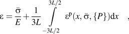 $$\varepsilon = {{\bar \sigma } \over E} + {1 \over {3L}}\int\limits_{{{ - 3L} \mathord{\left/ {\vphantom {{ - 3L} 2}} \right. \kern-\nulldelimiterspace} 2}}^{{{3L} \mathord{\left/ {\vphantom {{3L} 2}} \right. \kern-\nulldelimiterspace} 2}} {{\varepsilon ^{\rm{p}}}\left( {x,\bar \sigma ,\{ P\} } \right)} {\rm{d}}x\quad ,$$
to calculate, for a given stress, the corresponding total strain.
IV. DETERMINATION OF MODEL PARAMETERS
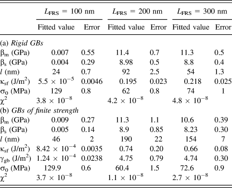
The parameters of the gradient plasticity model are determined by fitting the strain profiles calculated from the gradient plasticity to the plastic strain profiles with the same average strains that have been obtained from the DDD simulations (Figs. 3–5). To determine a set of parameters, sets of strain profiles corresponding to a given dislocation source length but with different average strains are fitted simultaneously. When considering strain profiles without GB yielding, the fit parameters are the yield stress σ0, the internal length scale ℓ, the hardening moduli βm and βs, and the surface parameter γsf. We assume that these parameters do not change during deformation (i.e., they are not dependent on the plastic strain); hence, all of the plastic strain profile curves for a given DDD profile series (corresponding to a given source length) share the same fit parameters. The procedure for GBs yielding at finite strain is analogous; however, in this case the GB parameter γgb is considered as an additional fit parameter. A comparison between the DDD data and the fitted gradient plasticity profiles is shown in Figs. 3(a)–5(a) for strain profiles without GB yielding, and in Figs. 3(b)–5(b) for strain profiles with GB of finite strength. The values of all fitted parameters are summarized in Table I.
Fit parameters and the corresponding standard error for tricrystals with different dislocation source lengths.
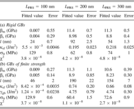
The quality of the fits has been evaluated in terms of the mean square deviation of the DDD and gradient plasticity strain profiles, evaluated at the discrete points representing the DDD profiles and with all profiles considered in the fit process for a given source length weighted equally. As demonstrated by the resulting χ2 values (mean square deviations between the DDD profiles and the fitted gradient plasticity strain profiles) as given in Table I, the assumption of GB yielding in general provides a significantly better fit to the data.
V. DISCUSSION AND CONCLUSIONS
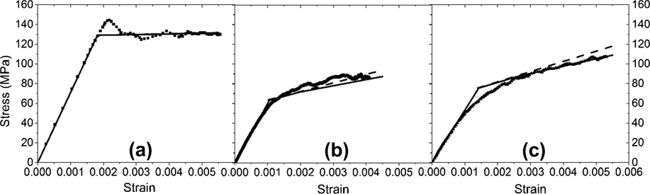
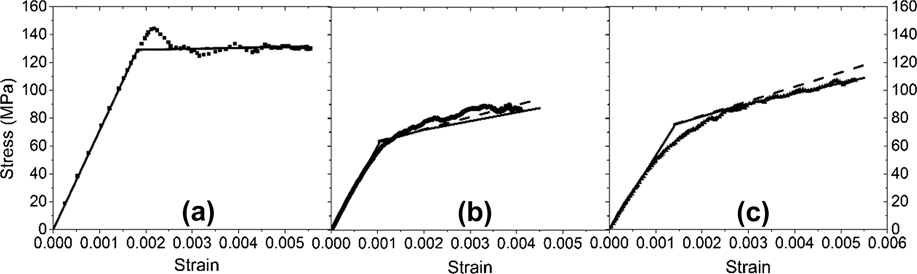
To assess the quality of the SG model, it is interesting to compare the DDD stress–strain curves with those derived from the gradient model using the fitted parameters given in Table I. With the exception of the effective elastic modulus E, global stress–strain data have not been used in our parameter fits, which exclusively rely on the plastic strain profiles to determine the constitutive parameters for the gradient plasticity model. Comparison of DDD and gradient plasticity stress–strain curves therefore provides an independent means for validating the gradient plasticity model. This is done in Figs. 7(a)–7(c), which juxtapose the DDD stress–strain data with those derived from gradient plasticity with and without GB yielding. It can be seen that, even though in our fitting procedure no attempt has been made to correctly reproduce the hardening curves, the qualitative differences in the hardening behavior between the tricrystals with different source lengths are actually reproduced very well by the gradient model. This indicates that the gradient model, despite its intrinsic simplicity, is actually capable of capturing the essential features of the interplay between dislocation motion, strain patterning, and strain hardening.
Comparison of stress–strain curves obtained from DDD and from gradient plasticity; (a) source length 100 nm, (b) source length 200 nm, and (c) source length 300 nm; data points: DDD, dashed lines: gradient plasticity with rigid GBs, and full lines: gradient plasticity with GBs of finite strength.
Examination of the values that the fits provide for ℓ, βm, βs and γgb leads to the following conclusions:
-
(1) For both rigid and penetrable GBs, the hardening modulus in the middle grain is always larger than that in the surface grains, i.e., βm > βs. This is reasonable since there is a strong GB constraint in the middle grain, leading to enhanced retention of dislocations, as opposed to free end surfaces in the surface grains where dislocations can leave the specimen.
-
(2) We do not find a monotonic dependence of the internal length parameter on dislocation source length. Since the mean source spacing was kept constant, a larger source length implies reduced dislocation spacing. We thus also do not find a monotonic dependence of the internal length parameter on dislocation spacing. From this we conclude that neither the source length, nor the source spacing, nor the dislocation spacing can universally be associated with the internal length scale of a gradient theory.
-
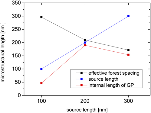
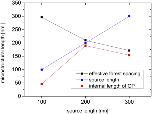
(3) Instead we need to ask which length scales control, in the three different cases investigated, the plastic flow process. As discussed in detail in Sec. II, in case of a source length of 100 nm, the relevant length scale is just the source length since the flow stress is controlled by source activation. In case of a source length of 300 nm, the relevant scale is the mean dislocation spacing of about 100 nm since the flow stress is controlled by dislocation–dislocation interactions. In the intermediate case, the source length of 200 nm and the dislocation spacing are of equal importance. Comparison with the fitted length scale parameters in Table I(b) indicates that both the nonmonotonic dependence of the length scale parameters and also their approximate magnitude can be readily explained if we make the physically reasonable assumption that the internal length scale parameter is, in each case, determined by the characteristic length which controls the flow stress, i.e., by the shorter of the source length and the dislocation spacing. This point, which is illustrated in Fig. 8, leads to an important conclusion: The two questions that concern the origin of the internal length scale, and the origin of the flow stress, are essentially equivalent. While no universally valid answer can be given, a physically correct understanding of the mechanism which controls, in a given situation, the deformation process will also yield an understanding of the associated length scale. Importantly, transitions between different hardening mechanisms may entail changes in the length scale parameter, and evolving internal length scales (e.g., a reduction in dislocation spacing in the course of strain hardening) may necessitate the assumption of strain-dependent internal lengths.
-
(4) Gradient plasticity is a phenomenological method to incorporate internal length scales into continuum plasticity theory. A physically based approach to the same end is continuum dislocation dynamics (CDD), i.e., the dynamics of dislocation densities. Reference Groma, Csikor and Zaiser25,Reference Hochrainer, Sandfeld, Zaiser and Gumbsch35 For dislocation systems that evolve under the action of their mutual interactions only, it has been shown Reference Zaiser and Sandfeld36 that the only internal length scale that can arise is the dislocation spacing. If, however, the dislocations interact with other defects, e.g., precipitates or radiation debris, these may control the flow stress through the dislocation source length, i.e., the initial dislocation radius of curvature, which then becomes an additional “extrinsic” length scale. While this feature cannot easily be captured in 2D CDD theories Reference Groma, Csikor and Zaiser25 curvature is contained naturally in recent 3D CDD approaches Reference Hochrainer, Sandfeld, Zaiser and Gumbsch35 which, accordingly, can predict transitions between different flow stress-controlling mechanisms as observed in the present manuscript. Gradient plasticity, of course, can always be adjusted to phenomenologically represent, but not to predict, such behavior.
-
(5) Our DDD data are best described in terms of a continuum model which allows for GB yielding – despite the fact that, in the DDD simulations, GBs were assumed to be completely impenetrable to dislocations. This leads to the important conclusion that the GB strength parameter in a gradient plasticity model may not necessarily represent an intrinsic property of the GB; rather, it should be considered as a phenomenological parameter that depends both on GB properties and on properties of the plastic flow processes on both sides of the boundary. In the present case, the GB yielding can be understood as the deposition of dislocations directly on the boundary. Since dislocations normally form smooth curves, deposition on the boundary implies discontinuities in line direction (high curvature at the points where the curved dislocations impinge on the boundary) which carry a high energy penalty. The resulting mean back force acting on a deposited segment is easily estimated in a line-tension approximation: It is proportional to the average angle at which dislocations impinge on the GB, which is in turn proportional to the SG at the boundary. This force must be compensated by Peach–Koehler forces exerted by dislocations on the opposite side of the boundary. Indeed, in our fits we find that the SG jumps across the GB at yield are almost the same for all three cases [Figs. 3–5(b)]. This is to be expected since the grain orientations, slip system activities, and hence the interactions of dislocations across the boundary are similar in all our simulations.
Correlation between the fitted GP length scale parameter (deformable GB case) and parameters of the dislocation microstructure.
To conclude, we have demonstrated that gradient plasticity provides a framework for capturing the interrelations between the strain heterogeneity and the hardening behavior in small systems. The same length scales that govern the hardening also control the width of the plastic boundary layers near the interfaces. Interface yielding through “dislocation condensation” on the interface may occur even if interfaces are physically impenetrable to dislocations. The associated strength parameters in this case reflect the interactions of dislocations across the boundaries, and are thus characteristic of the plastic flow processes on both the sides, rather than representing the intrinsic parameters of the boundary.
ACKNOWLEDGMENTS
The authors XZ, KEA, and MZ are grateful to the KEA's European Research Council Starting Grant MINATRAN 211166 for its support. XZ is grateful for the supports from the NSFC (11202172), the CPSF (2013M530405), and the Sichuan Provincial Youth Science and Technology Innovation Team (2013TD0004). MZ acknowledges the support under NSRF/ERC13 and GSRT/ARISTEIA II-SEDEMP. Finally, DW and MZ acknowledge the support by the Deutsche Forschungsgemeinschaft DFG-FG1650, grant WE3544/5-1, cofunded by the EPSRC under Grant No. Ep/J003387/1.