1 Introduction
Two-dimensional critical free-surface flow over a bottom topography produces a wide range of interesting and complex wave behaviour. Critical flow occurs when the Froude number based on the depth of water far upstream and downstream of a localised topography is equal to unity in both cases. The complex flow dynamics which is observed under unsteady conditions is well known, and the generic features include the formation of an undular bore and a periodic wavetrain downstream of a localised obstacle, as well as the recurrent emission of solitons which appear above the obstacle and then propagate upstream (see, for example, Grimshaw & Smyth Reference Grimshaw and Smyth1986; Smyth Reference Smyth1987; Wu Reference Wu1987; Ee et al. Reference Ee, Grimshaw, Zhang and Chow2010). Such features may be undesirable in certain situations as the waves which are generated can damage and erode the banks of waterways (e.g. Ellis et al. Reference Ellis, Sherman, Bauer and Hart2002; Bishop Reference Bishop2004; Bishop & Chapman Reference Bishop and Chapman2004). This motivates the further exploration and understanding of this important critical flow problem and, in particular, a consideration of the possible steady solutions and their stability.
In this study we investigate critical free-surface flow over a Gaussian dip topography. Both weakly nonlinear results computed as solutions to the forced Korteweg–de Vries (fKdV) equation, and fully nonlinear results, obtained as solutions to the full water-wave problem, are presented. Flow over a rectilinear dip topography has been discussed by Ee et al. (Reference Ee, Grimshaw, Zhang and Chow2010) and Keeler (Reference Keeler2017) using phase-plane methods. However, such methods are not available in the case of a smoothly varying topography. We investigate steady solutions, and in particular examine non-uniqueness of steady solutions, for the Gaussian topography under critical flow conditions using a combination of analytical and numerical methods. In the context of the fKdV equation, we also discuss the stability of these solutions via eigenvalue computations and by computing time-dependent solutions to the initial value problem.
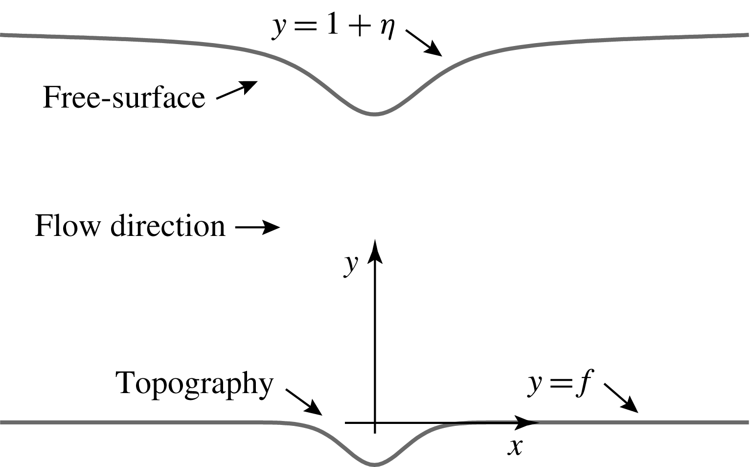
Sketch of the non-dimensional flow problem.

A sketch of the flow problem is shown in figure 1. It is assumed that the flow approaches a uniform stream of constant depth
 $H$
and speed
 $U$
as
 $x^{\ast }\rightarrow \pm \infty$
. The flow is characterised by the dimensionless Froude number
 $$\begin{eqnarray}F=\frac{U}{\sqrt{gH}},\end{eqnarray}$$
which represents the ratio of the characteristic flow speed
 $U$
to the maximum linear wave speed
 $\sqrt{gH}$
in a channel of finite depth, where
 $g$
is the magnitude of acceleration due to gravity; critical flow occurs when
 $F=1$
. The free surface is located at
 $y^{\ast }=H+\unicode[STIX]{x1D702}^{\ast }(x^{\ast },t^{\ast })$
, where the free-surface elevation
 $\unicode[STIX]{x1D702}^{\ast }$
is to be found as part of the solution to the problem. In terms of unstarred non-dimensional variables based on the length scale
 $H$
and time scale
 $\sqrt{H/g}$
, the fKdV equation takes the form (Akylas Reference Akylas1984; Wu Reference Wu1987)
 $$\begin{eqnarray}\unicode[STIX]{x1D702}_{t}+(F-1)\unicode[STIX]{x1D702}_{x}-{\textstyle \frac{3}{2}}\unicode[STIX]{x1D702}\unicode[STIX]{x1D702}_{x}-{\textstyle \frac{1}{6}}\unicode[STIX]{x1D702}_{xxx}={\textstyle \frac{1}{2}}\,f_{x},\end{eqnarray}$$
where
 $f(x)$
represents a general topographic forcing. We assume that this takes the form of a Gaussian which is symmetric about
 $x=0$
, and, moreover, we seek steady solutions for the free-surface shape which possess the same symmetry. More generally, when discussing the stability of these solutions, asymmetric free-surface profiles must be allowed for, and to this end we will assume in the far field the boundary conditions
 $$\begin{eqnarray}\unicode[STIX]{x1D702},\,\unicode[STIX]{x1D702}_{x},\,\unicode[STIX]{x1D702}_{xx}\rightarrow 0\quad \text{as }|x|\rightarrow \infty .\end{eqnarray}$$
As noted above, our focus is on the case
 $F=1$
for (1.2). For a negative point-force topography corresponding to a delta function forcing, a phase-plane analysis along the lines of Dias & Vanden-Broeck (Reference Dias and Vanden-Broeck2002) can be used to establish a unique steady solution to (1.2), (1.3) which decays algebraically in the far field. However, in the case of a smoothly varying topography, more than one steady solution is possible. This was demonstrated numerically by Binder, Blyth & Balasuriya (Reference Binder, Blyth and Balasuriya2014). We demonstrate analytically that our steady critical flow solutions decay algebraically in the far field. We note that in general when
 $F\neq 1$
exponential far-field decay is expected, as is discussed below.
It is worth emphasising that the results we present for the fKdV equation have wider applicability than to free-surface flows. Indeed, the fKdV equation has been discussed in the context of a wide range of physical scenarios. One application of particular importance, and which is of direct relevance to the present work, concerns internal waves in a stratified flow when the pycnocline, that is the interface between regions of different density, as may occur in atmospheric flow over ground relief (see, for example, Baines Reference Baines1977, Reference Baines1984; Malanotte-Rizzoli Reference Malanotte-Rizzoli1984; Grimshaw & Smyth Reference Grimshaw and Smyth1986).
2 Flow over a Gaussian dip
A necessary condition for a steady solution at
 $F=1$
can be found by integrating the steady form of (1.2) and applying the boundary conditions (1.3) to obtain
 $$\begin{eqnarray}\int _{-\infty }^{\infty }f(x)\hspace{2.22198pt}\text{d}x\leqslant 0.\end{eqnarray}$$
This shows that there are no steady solutions for non-trivial topography which is everywhere non-negative with
 $f(x)\geqslant 0$
for all
 $x$
. However, steady solutions may exist for any topography satisfying (2.1) including a Gaussian dip. Henceforth we adopt this form, taking
 $f(x)=a\exp (-b^{2}x^{2})$
for real constants
 $a<0$
and
 $b$
.
We rewrite the problem in terms of a single parameter by making the change of variables
 $\unicode[STIX]{x1D702}=2/9b^{2}u$
and
 $\unicode[STIX]{x1D709}=xb$
. Then the steady form of (1.2), after one integration, takes the form
 $$\begin{eqnarray}u_{\unicode[STIX]{x1D709}\unicode[STIX]{x1D709}}+u^{2}-\tilde{F}u=\unicode[STIX]{x1D6FC}\text{e}^{-\unicode[STIX]{x1D709}^{2}},\end{eqnarray}$$
where
 $\unicode[STIX]{x1D6FC}=-27a/(2b^{4})>0$
and
 $\tilde{F}=(6/b^{2})(F-1)$
. We note that in the limit
 $|\unicode[STIX]{x1D709}|\rightarrow \infty$
, wherein
 $u\rightarrow 0$
, there is a balance between the first and third terms on the left-hand side of (2.2) producing exponential far-field decay; however, when
 $F=1$
the balance is between the first and second terms yielding algebraic far-field decay. To summarise we seek solutions to (2.2) in the specific case
 $F=1$
, namely
 $$\begin{eqnarray}u_{\unicode[STIX]{x1D709}\unicode[STIX]{x1D709}}+u^{2}=\unicode[STIX]{x1D6FC}\text{e}^{-\unicode[STIX]{x1D709}^{2}},\end{eqnarray}$$
subject to the boundary conditions
 $$\begin{eqnarray}u_{\unicode[STIX]{x1D709}}(0)=0,\quad \lim _{\unicode[STIX]{x1D709}\rightarrow \infty }u=0.\end{eqnarray}$$
Note that by adopting the former boundary condition we seek only solutions which are even in
 $\unicode[STIX]{x1D709}$
. We begin by examining the extreme cases
 $\unicode[STIX]{x1D6FC}\ll 1$
and
 $\unicode[STIX]{x1D6FC}\gg 1$
.
2.1 The case
 $\unicode[STIX]{x1D6FC}\ll 1$

Working on the assumption that
 $\unicode[STIX]{x1D6FC}$
is small, we seek an asymptotic solution to (2.3) in the form
 $$\begin{eqnarray}u(\unicode[STIX]{x1D709})=\unicode[STIX]{x1D6FC}^{2/3}u_{0}(\unicode[STIX]{x1D709})+\unicode[STIX]{x1D6FC}u_{1}(\unicode[STIX]{x1D709})+\unicode[STIX]{x1D6FC}^{4/3}u_{2}(\unicode[STIX]{x1D709})+\cdots\end{eqnarray}$$
Substituting (2.5) into (2.3) and solving at successive orders of approximation using the first of the conditions in (2.4), we find
 $$\begin{eqnarray}u_{0}(\unicode[STIX]{x1D709})=\overline{u}_{0},\quad u_{1}(\unicode[STIX]{x1D709})=\int _{0}^{\unicode[STIX]{x1D709}}\unicode[STIX]{x1D707}(\unicode[STIX]{x1D70F})\hspace{2.22198pt}\text{d}\unicode[STIX]{x1D70F}+\overline{u}_{1},\quad u_{2}(\unicode[STIX]{x1D709})=-{\textstyle \frac{1}{2}}\overline{u}_{0}^{2}\unicode[STIX]{x1D709}^{2}+\overline{u}_{2},\end{eqnarray}$$
where the
 $\overline{u}_{i}$
are constants of integration, and
 $\unicode[STIX]{x1D707}(\unicode[STIX]{x1D70F})=\int _{0}^{\unicode[STIX]{x1D70F}}\text{exp}(-{\unicode[STIX]{x1D70F}^{\prime }}^{2})\hspace{2.22198pt}\text{d}\unicode[STIX]{x1D70F}^{\prime }$
. In the far field we find that
 $$\begin{eqnarray}u(\unicode[STIX]{x1D709})\sim \unicode[STIX]{x1D6FC}^{2/3}\overline{u}_{0}+\unicode[STIX]{x1D6FC}\left(\frac{\sqrt{\unicode[STIX]{x03C0}}}{2}\,\unicode[STIX]{x1D709}+\overline{u}_{1}-\frac{1}{2}\right)+O(\unicode[STIX]{x1D6FC}^{4/3})\end{eqnarray}$$
as
 $\unicode[STIX]{x1D709}\rightarrow \infty$
, which indicates that the expansion will fail when
 $\unicode[STIX]{x1D709}\sim O(\unicode[STIX]{x1D6FC}^{-1/3})$
. Accordingly we introduce an outer region in which the new variable
 $\unicode[STIX]{x1D701}=\unicode[STIX]{x1D6FC}^{1/3}\unicode[STIX]{x1D709}=O(1)$
and posit the expansion
 $u=\unicode[STIX]{x1D6FC}^{2/3}\tilde{u} _{0}(\unicode[STIX]{x1D701})+\cdots \,$
inside this outer region. Substituting into (2.3) we find at leading order and at first order,
 $$\begin{eqnarray}\tilde{u} _{0\unicode[STIX]{x1D701}\unicode[STIX]{x1D701}}+\tilde{u} _{0}^{2}=0,\quad \tilde{u} _{1\unicode[STIX]{x1D701}\unicode[STIX]{x1D701}}+2\tilde{u} _{0}\tilde{u} _{1}=0.\end{eqnarray}$$
The solutions which satisfy the second condition in (2.4) are
 $$\begin{eqnarray}\tilde{u} _{0}(\unicode[STIX]{x1D701})=-\frac{6}{(\unicode[STIX]{x1D701}+d_{1})^{2}},\quad \tilde{u} _{1}(\unicode[STIX]{x1D701})=\frac{d_{2}}{(\unicode[STIX]{x1D701}+d_{1})^{3}},\end{eqnarray}$$
where
 $d_{1}$
,
 $d_{2}$
are constants of integration. Matching to the inner region we find that
 $$\begin{eqnarray}\overline{u}_{0}=-\frac{6}{d_{1}^{2}},\quad d_{1}=2\left(\frac{3}{\sqrt{\unicode[STIX]{x03C0}}}\right)^{1/3},\end{eqnarray}$$
as well as
 $d_{2}=0$
and
 $\overline{u}_{1}=1/2$
. We conclude that for small
 $\unicode[STIX]{x1D6FC}$
, there exists a solution with negative elevation at the point of symmetry with
 $u(0)<0$
.
2.2 The case
$\unicode[STIX]{x1D6FC}\gg 1$

In this case it will be convenient to rescale the problem by introducing the new dependent variable
 $u=\unicode[STIX]{x1D6FC}^{1/2}U$
so that (2.3) takes the form
 $$\begin{eqnarray}\unicode[STIX]{x1D6FF}U_{\unicode[STIX]{x1D709}\unicode[STIX]{x1D709}}+U^{2}=\text{e}^{-\unicode[STIX]{x1D709}^{2}}\end{eqnarray}$$
where
 $\unicode[STIX]{x1D6FF}=\unicode[STIX]{x1D6FC}^{-1/2}$
and
 $\unicode[STIX]{x1D6FF}\ll 1$
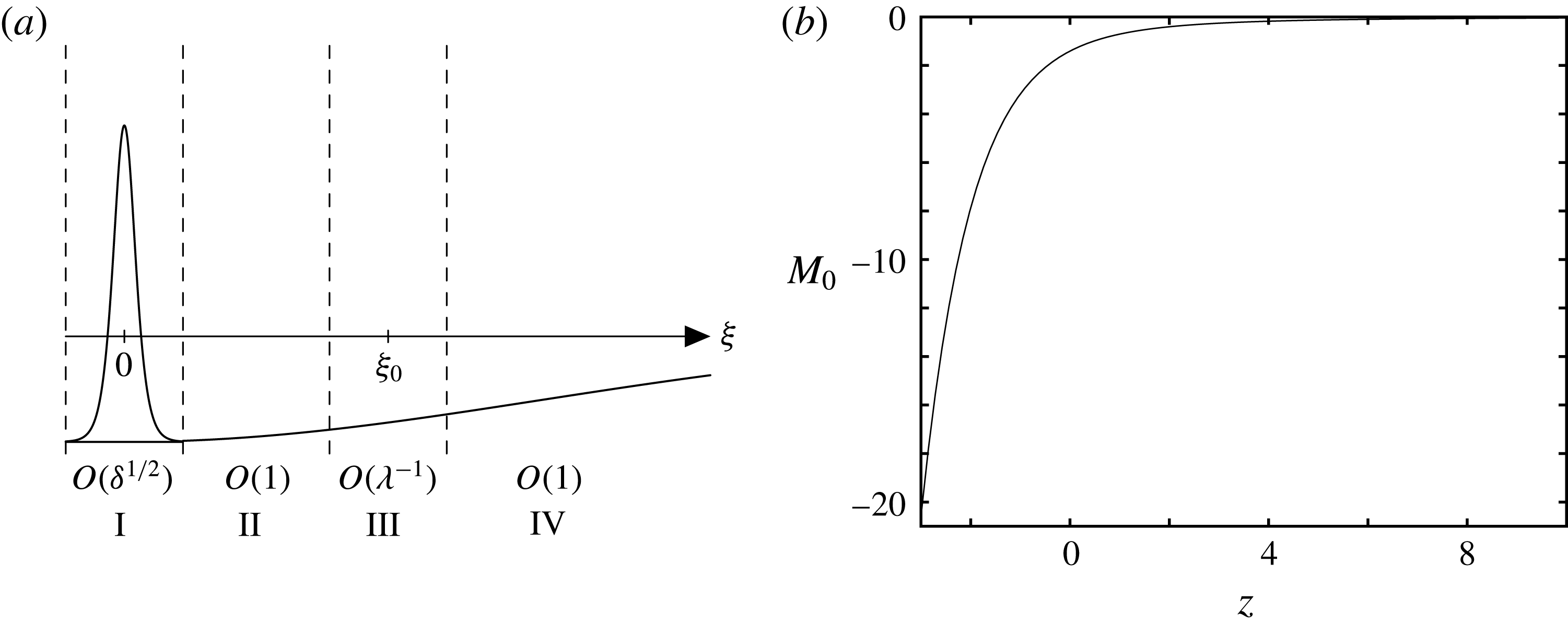
. Referring to figure 2 we see that the asymptotic solution for small
 $\unicode[STIX]{x1D6FF}$
has four distinct regions. In the core region, labelled region ii in the figure, we expand the solution by writing
 $$\begin{eqnarray}U=U_{0}+\unicode[STIX]{x1D6FF}U_{1}+\unicode[STIX]{x1D6FF}^{2}U_{2}+\unicode[STIX]{x1D6FF}^{3}U_{3}+\cdots \,.\end{eqnarray}$$
Substituting into (2.11) we obtain algebraic equations for the
 $U_{i}$
at successive orders of approximation which are solved easily. At leading order we find
 $$\begin{eqnarray}U_{0}=\pm \text{e}^{-\unicode[STIX]{x1D709}^{2}/2}.\end{eqnarray}$$
Discussion of the choice of the sign in (2.13) will be given below. At
 $O(\unicode[STIX]{x1D6FF})$
we have
 $$\begin{eqnarray}U_{1}=-\frac{U_{0\unicode[STIX]{x1D709}\unicode[STIX]{x1D709}}}{2U_{0}}=\frac{1}{2}(1-\unicode[STIX]{x1D709}^{2}),\end{eqnarray}$$
which is valid regardless of the sign taken for
 $U_{0}$
in (2.13). From the next two orders, we determine the forms
 $$\begin{eqnarray}U_{2}=\pm {\textstyle \frac{1}{8}}(\unicode[STIX]{x1D709}^{4}-2\unicode[STIX]{x1D709}^{2}-3)\text{e}^{\unicode[STIX]{x1D709}^{2}/2},\quad U_{3}={\textstyle \frac{5}{8}}(\unicode[STIX]{x1D709}^{4}-1)\text{e}^{\unicode[STIX]{x1D709}^{2}}.\end{eqnarray}$$
Although each of the
 $U_{i}$
in (2.12) satisfies the symmetry condition
 $U_{i\unicode[STIX]{x1D709}}(0)=0$
required by (2.4), the expansion must nonetheless break down as
 $\unicode[STIX]{x1D709}\rightarrow 0$
since the first term on the left-hand side of (2.11) will become comparable to the second in this limit. Moreover, (2.12) evidently breaks down as
 $\unicode[STIX]{x1D709}$
increases since successive terms in the expansion grow to become comparable in size to their predecessors. We address the first of these issues first, and consider the solution in the boundary layer at
 $\unicode[STIX]{x1D709}=0$
, namely region i in figure 2.


In region i, we introduce the boundary-layer variable
 $y=\unicode[STIX]{x1D6FF}^{-1/2}\unicode[STIX]{x1D709}$
and expand the solution by writing
 $$\begin{eqnarray}U=\tilde{U} _{0}(y)+\unicode[STIX]{x1D6FF}\tilde{U} _{1}(y)+\unicode[STIX]{x1D6FF}^{2}\tilde{U} _{2}(y)+\cdots \,.\end{eqnarray}$$
Substituting into (2.11), at leading order we find
 $$\begin{eqnarray}\tilde{U} _{0yy}+\tilde{U} _{0}^{2}=1\end{eqnarray}$$
subject to the symmetry condition
 $\tilde{U} _{0y}(0)=0$
and the condition that
 $\tilde{U} _{0}\sim \pm 1$
as
 $y\rightarrow \infty$
to match with region ii, the choice of sign in the latter condition being dictated by the choice of sign taken in (2.13). This problem has three possible solutions given by
 $$\begin{eqnarray}(\text{i})\quad \tilde{U} _{0}=1,\quad (\text{ii})\quad \tilde{U} _{0}=-1,\quad (\text{iii})\quad \tilde{U} _{0}=-1+3\operatorname{sech}^{2}(y/\sqrt{2}).\end{eqnarray}$$
Referring to the
 $(\tilde{U} _{0},\tilde{U} _{0y})$
phase plane, these correspond respectively to fixed points at
 $\tilde{U} _{0}=\pm 1$
, and a homoclinic orbit encircling
 $\tilde{U} _{0}=1$
which connects
 $\tilde{U} _{0}=-1$
to itself.
We examine cases (i) and (ii) first. At
 $O(\unicode[STIX]{x1D6FF})$
we have
 $$\begin{eqnarray}\tilde{U} _{1yy}\pm 2\tilde{U} _{1}=-y^{2}.\end{eqnarray}$$
The solution which satisfies
 $\tilde{U} _{1y}(0)=0$
, and which does not grow exponentially as
 $y\rightarrow \infty$
, is given by
 $$\begin{eqnarray}\tilde{U} _{1}={\textstyle \frac{1}{2}}(1\mp y^{2}).\end{eqnarray}$$
Since the expressions in (2.20) are forced directly by the solution in the core region ii, the matching with that region is immediate. For case (iii), we have
 $$\begin{eqnarray}\tilde{U} _{1yy}+2\big(3\operatorname{sech}^{2}(y/\sqrt{2})-1\big)\tilde{U} _{1}=-y^{2}.\end{eqnarray}$$
By making the change of variables
 $t=\tanh (y/\sqrt{2})$
, this can be transformed into the associated Legendre equation
 $$\begin{eqnarray}\frac{\text{d}}{\text{d}t}\left((1-t^{2})\frac{\text{d}\tilde{U} _{1}}{\text{d}t}\right)+\left(12-\frac{4}{1-t^{2}}\right)\tilde{U} _{1}=-\frac{4\operatorname{arctanh}^{2}t}{1-t^{2}}.\end{eqnarray}$$
The solution which satisfies the required symmetry condition
 $\tilde{U} _{1t}(0)=0$
is given by
 $$\begin{eqnarray}\displaystyle \tilde{U} _{1}(t) & = & \displaystyle \frac{1}{4}p_{1}(t)\left[\int _{0}^{t}\frac{\operatorname{arctanh}^{2}s}{s^{2}-1}\,p_{2}(s)\,\text{d}s-\frac{15}{2}\unicode[STIX]{x03C0}^{2}\right]+\frac{1}{32}\,p_{2}(t)\Bigg[4\log (1-t^{2})\nonumber\\ \displaystyle & & \displaystyle -\log \left(\frac{1+t}{1-t}\right)\left\{(1-t^{2})\log \left(\frac{1+t}{1-t}\right)-4t\right\}-8\log 2\Bigg],\end{eqnarray}$$
where
 $$\begin{eqnarray}p_{1}(t)=t(t^{2}-1),\quad p_{2}(t)=15t(t^{2}-1)\log \left(\frac{1+t}{1-t}\right)+\frac{50t^{2}-30t^{4}-16}{t^{2}-1}\end{eqnarray}$$
are the homogenous solutions to (2.22). We note that
 $\tilde{U} _{1}(t)\sim \operatorname{arctanh}^{2}t$
as
 $t\rightarrow 1$
and so
 $\tilde{U} _{1}\sim y^{2}/2$
ensuring a match with region ii.
We now turn our attention to region iii. Scrutinising the terms
 $U_{0}$
and
 $U_{1}$
in (2.13) and (2.14), we see that the expansion (2.12) in region ii breaks down when
 $\exp (-\unicode[STIX]{x1D709}^{2}/2)\sim 1/2\unicode[STIX]{x1D6FF}(\unicode[STIX]{x1D709}^{2}-1)$
. This occurs when
 $\unicode[STIX]{x1D709}\sim \unicode[STIX]{x1D709}_{0}(\unicode[STIX]{x1D6FF})$
, where
 $$\begin{eqnarray}\unicode[STIX]{x1D709}_{0}=\unicode[STIX]{x1D706}-\unicode[STIX]{x1D706}^{-1}\log (\unicode[STIX]{x1D706}^{2}/2)+\cdots \,,\end{eqnarray}$$
with
 $\unicode[STIX]{x1D706}=(-2\log \unicode[STIX]{x1D6FF})^{1/2}$
. Inside this narrow region, we introduce the internal layer variable
 $z=\unicode[STIX]{x1D706}(\unicode[STIX]{x1D709}-\unicode[STIX]{x1D709}_{0})$
, and expand by writing
 $$\begin{eqnarray}\displaystyle U=\unicode[STIX]{x1D6FF}\unicode[STIX]{x1D706}^{2}M_{0}(z)+\unicode[STIX]{x1D6FF}M_{1}(z)+\cdots \,. & & \displaystyle\end{eqnarray}$$
Substituting into equation (2.11), we obtain at leading order,
 $$\begin{eqnarray}M_{0zz}+M_{0}^{2}=\text{e}^{-2z}.\end{eqnarray}$$
The boundary conditions are
 $$\begin{eqnarray}\lim _{z\rightarrow -\infty }M_{0}=\pm \infty ,\quad \lim _{z\rightarrow \infty }M_{0}=0.\end{eqnarray}$$
Here the
 $+/-$
sign is required to match to the solution in region ii, namely (2.13) with the
 $+/-$
sign selected respectively. It is possible to compute a solution to this problem numerically for either choice of sign; however, great care is needed when attempting to match the solution with region ii, as will be discussed below. We discuss first the case of the minus sign in (2.28). Figure 2 shows the result of a calculation using fourth-order Runge–Kutta integration to solve the problem (2.27) with the minus sign chosen in the boundary condition (2.28). An analysis for large negative
 $z$
reveals that the solution takes the form
 $$\begin{eqnarray}M_{0}(z)=-\text{e}^{-z}-{\textstyle \frac{1}{2}}+{\textstyle \frac{1}{8}}\text{e}^{z}+c_{1}\text{K}_{2}(2\sqrt{2}\,\text{e}^{-z/2})+\cdots\end{eqnarray}$$
as
 $z\rightarrow -\infty$
, where
 $\text{K}_{2}$
is a modified Bessel function of the second kind, and
 $c_{1}$
is a constant which must be determined globally but is not required here. Since it is known that
 $\text{K}_{2}(w)\sim \sqrt{\unicode[STIX]{x03C0}/2z}\,\text{exp}(-2z)\cdots \,$
(e.g. Abramowitz & Stegun Reference Abramowitz and Stegun1964), the final term in (2.29) decays superexponentially and matching to region ii is possible. For large positive
 $z$
, the forcing term on the right-hand side of (2.27) becomes negligible and the dominant balance of the two terms on the left-hand side requires the behaviour
 $M_{0}\sim -6/(z+c_{2})^{2}$
, for constant
 $c_{2}$
, as
 $z\rightarrow \infty$
. In region iv, the expansion proceeds as
 $$\begin{eqnarray}U(\unicode[STIX]{x1D709})=\unicode[STIX]{x1D6FF}\hat{U} _{0}(w)+\cdots \,,\end{eqnarray}$$
where
 $w=\unicode[STIX]{x1D709}-\unicode[STIX]{x1D709}_{0}=O(1)$
. At leading order we have
 $\hat{U} _{0ww}+U_{0}^{2}=0$
and the solution satisfying the far-field condition in (2.4), namely
 $\hat{U} _{0}\rightarrow 0$
as
 $w\rightarrow \infty$
, is
 $$\begin{eqnarray}\hat{U} _{0}=-\frac{6}{(w+c_{3})^{2}},\end{eqnarray}$$
for constant
 $c_{3}$
which can in principle be found by matching to region iii.
As noted above, it is possible to numerically compute a solution to the problem (2.27) subject to (2.28) with the plus sign selected in the boundary condition. However, the numerical solution exhibits small decaying oscillations for large negative
 $z$
. Indeed, in the limit
 $z\rightarrow -\infty$
it can be shown that
 $$\begin{eqnarray}M_{0}(z)\sim \text{e}^{-z}-{\textstyle \frac{1}{2}}-{\textstyle \frac{1}{8}}\text{e}^{z}+\unicode[STIX]{x1D6FC}_{1}\text{J}_{2}(2\sqrt{2}\text{e}^{-z/2})+\unicode[STIX]{x1D6FC}_{2}\text{Y}_{2}(2\sqrt{2}\text{e}^{-z/2})+\cdots \,,\end{eqnarray}$$
for constants
 $\unicode[STIX]{x1D6FC}_{1}$
,
 $\unicode[STIX]{x1D6FC}_{2}$
, where
 $\text{J}_{2}$
and
 $\text{Y}_{2}$
are Bessel functions of the first and second kind respectively. As
 $\unicode[STIX]{x1D709}\rightarrow \infty$
,
 $\text{J}_{2}(\unicode[STIX]{x1D709})\sim \sqrt{2/\unicode[STIX]{x03C0}\unicode[STIX]{x1D709}}\,\cos (\unicode[STIX]{x1D709}-5\unicode[STIX]{x03C0}/4)+\cdots \,$
and
 $\text{Y}_{2}(\unicode[STIX]{x1D709})\sim \sqrt{2/\unicode[STIX]{x03C0}\unicode[STIX]{x1D709}}\,\sin (\unicode[STIX]{x1D709}-5\unicode[STIX]{x03C0}/4)+\cdots \,$
(Abramowitz & Stegun Reference Abramowitz and Stegun1964) and so
 $M_{0}$
has decaying oscillations as
 $z\rightarrow -\infty$
in agreement with the numerical solution. Since the solution in region ii is non-oscillatory, it is not possible to complete a match between regions ii and iii, and on this basis we must reject the choice of the plus sign in (2.13) since it does not lead to a consistent asymptotic solution.
We conclude that consistent asymptotic solutions may be constructed for cases (ii) and (iii) in (2.18), but not for case (i). This means that there are two asymptotic solutions consistent with the choice of a minus sign in (2.13), namely cases (ii) and (iii), but there are no solutions consistent with the choice of a plus sign in (2.13), namely case (i).
2.3 Numerical results
In summary, we have found in § 2.2 that it is possible to construct a consistent asymptotic solution using boundary-layer theory for cases (ii) and (iii) in (2.18), but not for case (i). This together with the results of the small
 $\unicode[STIX]{x1D6FC}$
asymptotic analysis in § 2.1 suggests that there exist at least two distinct branches of steady solutions. To carry out a full investigation of the solution space, we solved the steady problem (2.3) numerically employing a shooting technique based on the fourth-order Runge–Kutta method. The problem was first reformulated as a first-order system in the form
 $\boldsymbol{x}_{\unicode[STIX]{x1D709}}=\boldsymbol{F}(\boldsymbol{x})$
, where
 $\boldsymbol{x}=(u,u_{\unicode[STIX]{x1D709}})^{\text{T}}$
and
 $\boldsymbol{F}=(u_{\unicode[STIX]{x1D709}},\unicode[STIX]{x1D6FC}s-u^{2})^{\text{T}}$
. Following the assumed symmetry of the solution, the system was integrated forward from the starting point
 $\boldsymbol{x}(\unicode[STIX]{x1D709}=0)=(u_{0},0)^{\text{T}}$
for a chosen
 $u_{0}$
. The correct value of
 $u_{0}$
was determined iteratively until the trajectory of the solution in the
 $(u,u_{\unicode[STIX]{x1D709}})$
phase plane approaches the origin. Formally this should happen in infinite time as
 $\unicode[STIX]{x1D709}\rightarrow \infty$
but in computational practice the value of
 $u_{0}$
was refined so that an increasingly large value of
 $\unicode[STIX]{x1D709}$
was required to reach the origin. There are two qualitatively different ways in which this can happen as follows:
 $$\begin{eqnarray}(a)\quad \frac{u_{\unicode[STIX]{x1D709}}}{u}\sim -\frac{2}{\unicode[STIX]{x1D709}}\quad \text{or}\quad (b)\quad \frac{u_{\unicode[STIX]{x1D709}}}{u}\sim -2\unicode[STIX]{x1D709}\end{eqnarray}$$
as
 $\unicode[STIX]{x1D709}\rightarrow \infty$
. Option (a) represents a balance between the two terms on the left-hand side of (2.3) and constitutes algebraic decay of the solution as
 $-6\unicode[STIX]{x1D709}^{-2}$
for large
 $\unicode[STIX]{x1D709}$
. In this case the slope of the trajectory tends to
 $0-$
as the origin is approached. Option (b) represents a balance between the first term on the left-hand side of (2.3) and the topographic forcing term on the right-hand side. In this case the trajectory enters the origin from below with an infinitely negative slope. The computed solution was checked against an independent calculation in which the boundary value problem was solved using a finite difference method on a uniform grid over the truncated domain
 $[-L,L]$
with
 $L$
taken to be suitably large. Approximating the second derivative in (2.3) with a centred difference furnishes a set of nonlinear algebraic equations at each grid point, which were solved using Newton’s method.
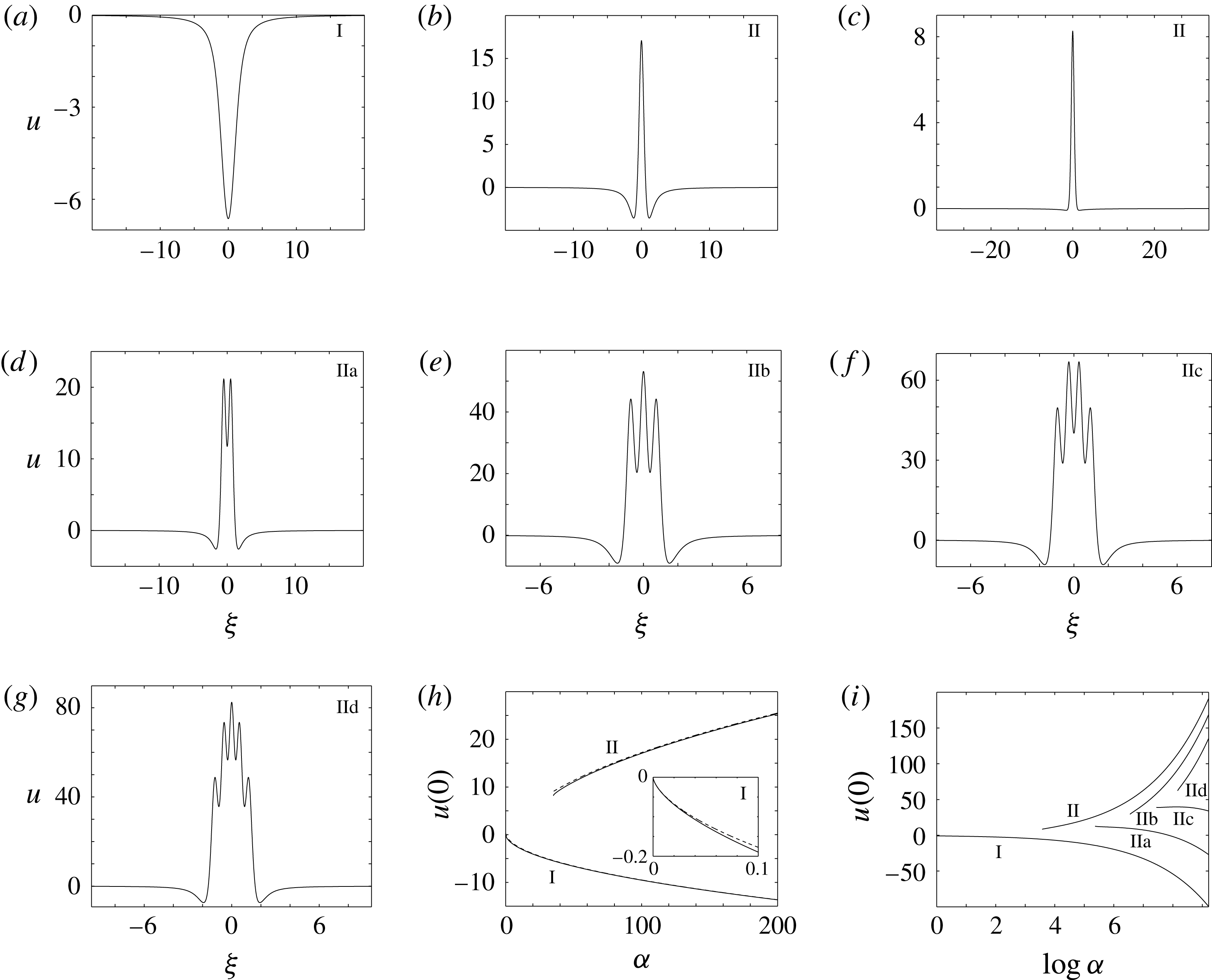
Figure 3(a–c) shows numerical computations of the two solution types predicted by the asymptotic analysis. We refer to the depression wave in figure 3(a) as a type i solution and the elevation waves in figure 3(b,c) as type ii solutions. The solution space, characterised by the value
 $u(0)$
, is shown in figures 3(h) and 3(i). The predictions of the asymptotic analysis are included in figures 3(h) and 3(i). Numerically, we find that the far-field behaviour (a) in (2.33) is obtained on the lower branch of type i solutions and also on almost all of the upper branch except at the point
 $\unicode[STIX]{x1D6FC}\approx 35.14$
, where this branch terminates and where the numerical evidence appears to suggest that behaviour (b) occurs. Further experimentation revealed the existence of a seemingly infinite sequence of new solutions iia,b,c,d etc., which are not predicted by our asymptotic analysis, and which have oscillations on the free surface localised around the origin. Examples are shown in figure 3(d–g). We note the similarity with the solution space over a rectangular trench (Keeler Reference Keeler2017).
(a–g) Free-surface profiles: (a) type i at
 $\unicode[STIX]{x1D6FC}=50$
; (b) type ii at
 $\unicode[STIX]{x1D6FC}=100$
; (c) type ii at
 $\unicode[STIX]{x1D6FC}=35.2$
, close to the branch termination point; (d) type iia at
 $\unicode[STIX]{x1D6FC}=300$
; (e) type iib at
 $\unicode[STIX]{x1D6FC}=1500$
; (f) type iic at
 $\unicode[STIX]{x1D6FC}=3000$
; (g) type iid at
 $\unicode[STIX]{x1D6FC}=5000$
. (h) Solution space. The large
 $\unicode[STIX]{x1D6FC}$
behaviour
 $u(0)\sim -\unicode[STIX]{x1D6FC}^{1/2}+1/2$
, case (ii) in (2.18), is shown with a broken curve overlaid on the lower branch. The broken curve overlaid on the upper branch is the large
 $\unicode[STIX]{x1D6FC}$
behaviour for the type ii solution
 $u(0)\sim 2\unicode[STIX]{x1D6FC}^{1/2}-4\log (2)$
, case (iii) in (2.18). The inset shows behaviour for small
 $\unicode[STIX]{x1D6FC}$
. The broken curve illustrates the small
 $\unicode[STIX]{x1D6FC}$
behaviour
 $u(0)\sim -(6/d_{1}^{2})\unicode[STIX]{x1D6FC}^{2/3}+(1/2)\unicode[STIX]{x1D6FC}$
, with
 $d_{1}$
as given in (2.10). (i) Extended view of the solution space including type iia, b, c and d solutions. The latter solutions terminate at
 $\unicode[STIX]{x1D6FC}\approx 214.0,\hspace{2.22198pt}699.1,\hspace{2.22198pt}1709.0$
and
 $3508.0$
respectively.

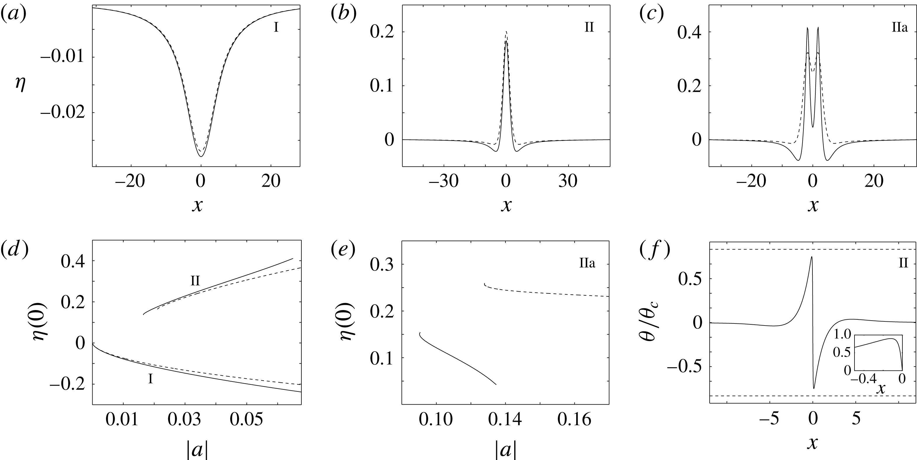
Fully nonlinear results for the Gaussian topography (solid curves),
 $b=0.3$
. The broken curves are for the weakly nonlinear solutions. (a) Type i solution,
 $a=-0.0017$
. (b) Type ii solution,
 $a=-0.039$
. (c) Type iia solution,
 $a=-0.134$
. (d) Solution space for the type i and ii solutions. (e) Solution space for the type iia solution. (f) Reduced surface angle
 $\unicode[STIX]{x1D703}/\unicode[STIX]{x1D703}_{c}$
, where
 $\unicode[STIX]{x1D703}_{c}=\unicode[STIX]{x03C0}/6$
, for the highest computed type ii wave at
 $a=-0.06484$
. In (f) the inset shows a close-up near to
 $x=0$
.

2.4 Fully nonlinear calculations
We now compare the results obtained for the weakly nonlinear model to those found for the fully nonlinear problem. In the non-dimensionalised steady water-wave equations the velocity potential
 $\unicode[STIX]{x1D719}(x,y)$
satisfies Laplace’s equation throughout the flow domain,
 $$\begin{eqnarray}\unicode[STIX]{x1D6FB}^{2}\unicode[STIX]{x1D719}=0\quad \text{in }-\infty <x<\infty ,~f(x)<y<1+\unicode[STIX]{x1D702}(x).\end{eqnarray}$$
On the free surface the dynamic and kinematic boundary conditions need to be satisfied,
 $$\begin{eqnarray}\left.\begin{array}{@{}l@{}}\displaystyle \frac{1}{2}|\unicode[STIX]{x1D735}\unicode[STIX]{x1D719}|^{2}+\displaystyle \frac{1}{F^{2}}y=\displaystyle \frac{1}{2}+\displaystyle \frac{1}{F^{2}}\\ \unicode[STIX]{x1D702}_{x}\unicode[STIX]{x1D719}_{x}=\unicode[STIX]{x1D719}_{y}\end{array}\right\}\quad \text{on }y=1+\unicode[STIX]{x1D702}(x),\end{eqnarray}$$
along with the no-penetration condition on the bottom,
 $$\begin{eqnarray}f_{x}\unicode[STIX]{x1D719}_{x}=\unicode[STIX]{x1D719}_{y}\quad \text{on }y=f(x).\end{eqnarray}$$
We solved this system of equations for the unknown functions
 $\unicode[STIX]{x1D719}(x,y)$
and
 $\unicode[STIX]{x1D702}(x)$
at
 $F=1$
numerically for the Gaussian forcing
 $f(x)=a\exp (-b^{2}x^{2})$
with the aim of computing solitary wave solutions. Based on the weakly nonlinear analysis we would expect the tails of the solitary waves to decay algebraically, and indeed we establish analytically in appendix A that the full nonlinear solutions decay like
 $-(4/3)x^{-2}$
as
 $x\rightarrow \pm \infty$
, which is precisely the far-field behaviour found for the fKdV equation (2.3). Consequently a large truncation length for the computational domain is required for the computations. The numerical computations were performed first using the boundary-integral method described by Tam et al. (Reference Tam, Yu, Kelso and Binder2015) over the truncated domain
 $[-L,L]$
for chosen
 $L$
. Anticipating an inverse square algebraic decay in the far field, the boundary conditions
 $\unicode[STIX]{x1D702}_{x}/(1+\unicode[STIX]{x1D702})=\mp \,2/L$
were applied at
 $x=\pm L$
respectively. Second, the fully nonlinear system is first reformulated as a single partial differential equation with a non-local term in terms of surface variables alone, as described in appendix A. The resulting equation (A 11) together with (A 5) is solved with spectral accuracy over the truncated domain
 $[-L^{\prime },L^{\prime }]$
, for large
 $L^{\prime }$
in the mapped domain, assuming periodic boundary conditions, by employing the fast Fourier transform. In the results presented here the computations were done with the first of the numerical approaches, except for the type II branch solutions, where the second approach proved more expeditious particularly in obtaining the steep wave profiles.
The comparison with the weakly nonlinear solutions for the steady fKdV equation (2.3) is shown in figure 4(a–e). The type i solution demonstrates a very good agreement with a small discrepancy at the wave minimum. Note that only a portion of the wave is shown around the origin since the two solutions are visually indistinguishable over the remainder of the range. There is very good agreement on the type i solution branch for small
 $|a|$
as expected. The fully nonlinear type ii solution branch exhibits similar behaviour to the weakly nonlinear prediction but while the latter branch continues indefinitely through negative values of
 $a$
, the former terminates at a finite value of
 $a$
. We note that the fully nonlinear branch cannot possibly follow the weakly nonlinear branch for large
 $a$
since it is clear from the Bernoulli equation in (2.35) that the surface elevation is bounded above with
 $\unicode[STIX]{x1D702}\leqslant 1/2$
in the case
 $F=1$
; equality is obtained at a stagnation point where the first term in the Bernoulli equation vanishes. Such an eventuality is expected at the crest of a Stokes-limiting configuration, as is found for unforced solitary waves (e.g. Hunter & Vanden-Broeck Reference Hunter and Vanden-Broeck1983). We computed the branch up to
 $a=-0.06484$
(see figure 4
d) at which point a very large number of mesh points are required to obtain an accurate solution as the wave profile does indeed seem to be approaching a Stokes-limiting configuration with an interior angle of
 $120^{\circ }$
, and a stagnation point, at the crest. The surface angle
 $\unicode[STIX]{x1D703}$
, defined as the angle between the tangent to the surface and the horizontal, is shown in figure 4(f) for the type ii profile obtained at
 $a=-0.06484$
. This particular calculation was performed using the numerical method discussed above with
 $2^{14}=16\,384$
points equally spaced in the mapped domain with
 $L^{\prime }=100$
. Given the very high resolution required, we did not attempt to move further along the branch toward the Stokes-limiting configuration. Wade et al. (Reference Wade, Binder, Mattner and Denier2014) experienced similar numerical difficulties close to the Stokes-limiting configuration for an imposed distribution of pressure on the free surface. In the current work the algebraic far-field decay presents an added difficulty.
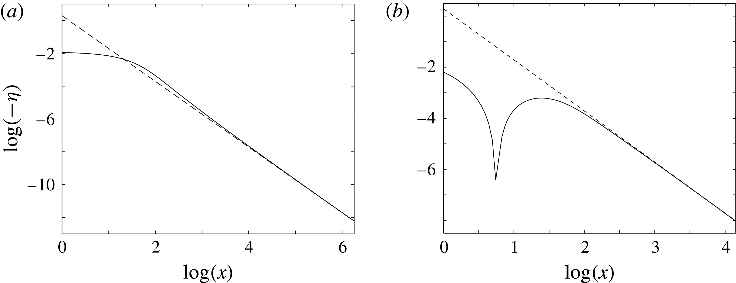
Far-field decay of fully nonlinear solutions for a Gaussian topography,
 $a=-0.03$
and
 $b=0.3$
, computed on domain
 $[-L^{\prime },L^{\prime }]$
with
 $2048$
collocation points using the method described in appendix A. Profiles for type i (a) and type ii (b) shown on a
 $\log$
-
 $\log$
plot. In both (a) and (b) the asymptote
 $\log (-\unicode[STIX]{x1D702})=\log (4/3)-2\log x$
is shown with a dashed line.

As was discussed in § 2.3, the weakly nonlinear branch terminates at its right-hand end at a negative value of
 $a$
, as can be seen in figure 4(d). We find that the fully nonlinear branch also appears to terminate at its right-hand end. Generally solutions along this fully nonlinear branch decay algebraically as
 $-(4/3)x^{-2}$
and this is confirmed in figure 5, which demonstrates excellent agreement between the analytic prediction and the numerical computation for a sample case along this branch. It is numerically extremely difficult to identify the shift from algebraic decay to exponential decay (behaviour (b) in (2.33)) which we anticipate will herald the end of the branch as it does for the weakly nonlinear theory.
The solution type iia also exists in the fully nonlinear solution space but there is a large difference between the fKdV and fully nonlinear solution branches (see figure 4
c,e) as might be expected since the amplitude
 $a$
is here rather large. It seems reasonable to suppose that the type iib,c,
 $\ldots$
branches are also present in the fully nonlinear regime but since they would likely be quantitatively quite different to their weakly nonlinear counterparts it may not be straightforward to find them, and we have not attempted to do so. We also note in common with the weakly nonlinear theory, the type iia branch terminates at its right-hand end; however as with the type ii solutions it appears also to terminate at its other end.
3 Stability and time-dependent behaviour of solutions
To conclude our study we examine the stability properties of the steady solutions. We construct conditions for the solutions to be stable using the Hamiltonian argument of Camassa & Wu (Reference Camassa and Wu1991) and complement these analytical results with careful numerical computations.
3.1 Stability analysis
The aim is to classify the steady solutions we have computed as being neutrally, spectrally, linearly or formally stable. For a definition of these terms, see for example, Holm et al. (Reference Holm, Marsden, Ratiu and Weinstein1985); however we will remind the reader of their precise meaning as the analysis proceeds.
Our starting point is the time-dependent fKdV equation (1.2) at the critical condition
 $F=1$
, which is repeated here for convenience,
 $$\begin{eqnarray}\unicode[STIX]{x1D702}_{t}-{\textstyle \frac{3}{2}}\unicode[STIX]{x1D702}\unicode[STIX]{x1D702}_{x}-{\textstyle \frac{1}{6}}\unicode[STIX]{x1D702}_{xxx}={\textstyle \frac{1}{2}}\,f_{x}(x).\end{eqnarray}$$
To investigate the stability we write
 $\unicode[STIX]{x1D702}(x,t)=\unicode[STIX]{x1D702}_{s}(x)+\unicode[STIX]{x1D716}\unicode[STIX]{x1D701}(x,t)$
, where
 $\unicode[STIX]{x1D702}_{s}$
is a steady solution of (3.1) and
 $\unicode[STIX]{x1D701}$
is a time-dependent perturbation, and where
 $\unicode[STIX]{x1D716}\ll 1$
. We demand that the perturbation
 $\unicode[STIX]{x1D701}$
satisfies the same far-field conditions as
 $\unicode[STIX]{x1D702}$
, namely equation (1.3). Substituting into (3.1) and retaining terms at
 $O(\unicode[STIX]{x1D716})$
we obtain
 $$\begin{eqnarray}\unicode[STIX]{x1D701}_{t}={\mathcal{M}}\unicode[STIX]{x1D701}=-\frac{\unicode[STIX]{x2202}}{\unicode[STIX]{x2202}x}({\mathcal{K}}\unicode[STIX]{x1D701}),\quad {\mathcal{K}}=-{\textstyle \frac{1}{6}}\unicode[STIX]{x2202}_{xx}-{\textstyle \frac{3}{2}}\unicode[STIX]{x1D702}_{s}.\end{eqnarray}$$
The general solution to (3.2) may be written in the form (e.g. Chang & Demekhin Reference Chang and Demekhin2002, § 7.3)
 $$\begin{eqnarray}\unicode[STIX]{x1D701}(x,t)=\mathop{\sum }_{k=1}^{N_{p}}a_{k}g_{k}(x)\,\text{e}^{s_{k}t}+\int _{\unicode[STIX]{x1D6E4}}a(s)g(x,s)\,\text{e}^{st}\,\text{d}s,\end{eqnarray}$$
where the
 $a_{k}$
and
 $a(s)$
are expansion coefficients corresponding respectively to the
 $N_{p}$
values of
 $s_{k}$
in the point spectrum and to the continuous spectrum of the operator
 ${\mathcal{M}}$
. These satisfy the relation
 $$\begin{eqnarray}{\mathcal{M}}g=sg,\end{eqnarray}$$
(with
 $k$
subscripts appended in the case of the point spectrum). The integral in the second term in (3.3) is taken over the contour
 $\unicode[STIX]{x1D6E4}$
which delineates the continuous spectrum in the complex
 $s$
plane. The eigenfunctions in the point spectrum,
 $g_{k}(x)$
, reside in
 $L_{2}(-\infty ,\infty )$
. Furthermore, they satisfy the integral constraint,
 $$\begin{eqnarray}\int _{-\infty }^{\infty }g_{k}(x)\,\text{d}x=0\quad (s\neq 0),\end{eqnarray}$$
which is obtained by integrating (3.4) over the real line and using the fact that
 $g_{k}\rightarrow 0$
as
 $|x|\rightarrow \infty$
(Camassa & Wu Reference Camassa and Wu1991). Consequently the eigenfunctions
 $g_{k}$
carry zero excess mass. The functions
 $g(x,s)$
associated with the continuous spectrum
 $\unicode[STIX]{x1D6E4}$
are bounded as
 $|x|\rightarrow \infty$
. The continuous spectrum itself is determined by examining the behaviour as
 $|x|\rightarrow \infty$
(e.g. Sandstede Reference Sandstede2002). In this limit, the second term in
 ${\mathcal{K}}$
defined in (3.2) can be neglected and (3.2) reduces to
 $\unicode[STIX]{x1D701}_{t}-(1/6)\unicode[STIX]{x1D701}_{xxx}=0$
; adopting the form
 $\unicode[STIX]{x1D701}=\text{exp}(st)g(x,s)$
, we find
 $g=\text{exp}(\text{i}kx)$
and
 $s=-\text{i}k^{3}/6$
for
 $k\in \mathbb{R}$
so that the continuous spectrum occupies the imaginary axis:
 $\unicode[STIX]{x1D6E4}=\{\text{i}q:q\in \mathbb{R}\}$
.
In the case of type i steady solutions, which have the property that
 $\unicode[STIX]{x1D702}_{s}(x)<0$
for all
 $x$
, it is straightforward to show that the point spectrum of
 ${\mathcal{M}}$
does not include the origin (Keeler Reference Keeler2017). In the case of type ii steady solutions, numerically computed spectra are found to not include the origin, as will be discussed below.
If there is no eigenvalue in the spectrum in the right-half-complex-plane, that is with a positive real part, then
 $\unicode[STIX]{x1D702}_{s}(x)$
is spectrally stable. If the spectrum is contained along the imaginary axis, then the solution is neutrally stable. The solution is linearly stable if for every
 $\unicode[STIX]{x1D716}>0$
there exists a
 $\unicode[STIX]{x1D6FF}>0$
such that if in a suitable norm
 $\Vert \unicode[STIX]{x1D701}(x,0)\Vert <\unicode[STIX]{x1D6FF}$
then
 $\Vert \unicode[STIX]{x1D701}(x,t)\Vert <\unicode[STIX]{x1D716}$
for
 $t>0$
. While linear stability clearly implies spectral stability, the converse is not necessarily true (see Holm et al. (Reference Holm, Marsden, Ratiu and Weinstein1985) for some examples). As was pointed out by Camassa & Wu (Reference Camassa and Wu1991), for a steady solution
 $\unicode[STIX]{x1D702}_{s}(x)$
which is even in
 $x$
(resulting from an even topography), the operator
 ${\mathcal{M}}$
is odd in
 $x$
, i.e.
 ${\mathcal{M}}g(-x)=-{\mathcal{M}}g(x)$
, which means that for each eigenvalue
 $s$
satisfying (3.4),
 $-s$
,
 $s^{\ast }$
and
 $-s^{\ast }$
are also eigenvalues, so that the spectrum has a fourfold symmetry in the complex plane. As a consequence, spectral stability can only occur if all of the eigenvalues lie on the imaginary axis, in which case the solution is neutrally stable. Therefore for the fKdV equation with even topography, neutral stability for even solutions is a necessary and sufficient condition for spectral stability.
We have computed the spectrum of the
 ${\mathcal{M}}$
operator numerically on a truncated domain
 $[-L,L]$
with periodic boundary conditions using a spectral method. Sandstede & Scheel (Reference Sandstede and Scheel2000) showed that calculations performed on a periodic domain faithfully reproduce the point and continuous spectra provided the size of the domain is large enough. Bridges, Derks & Gottwald (Reference Bridges, Derks and Gottwald2002) and Barashenkov & Zemlyanaya (Reference Barashenkov and Zemlyanaya2000) have noted that numerical algorithms for computing eigenvalues in KdV-type problems can lead to spurious eigenvalues leaving/entering the imaginary axis and posing as unstable/stable modes. With this in mind, we have performed careful convergence tests on our results and, furthermore, we confirm our results by comparison with time-dependent simulations to be discussed in the next subsection. For type i solutions the spectrum is found to be contained on the imaginary axis indicating that the flow is spectrally stable in this case. This conclusion will be confirmed via a formal argument to be presented below. In contrast type ii solutions are found numerically to be linearly unstable. In all cases we examined we found that the operator
 ${\mathcal{M}}$
has just one unstable eigenvalue
 $s$
in the right-half-plane (excluding
 $s^{\ast }$
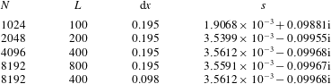
). In fact, this was found to be true for all of the type ii and type iia solutions shown in figure 3(h). Table 1 illustrates the convergence of the unstable eigenvalue for a sample type ii case as the discretisation level
 $N$
and the truncation length of the computational domain
 $L$
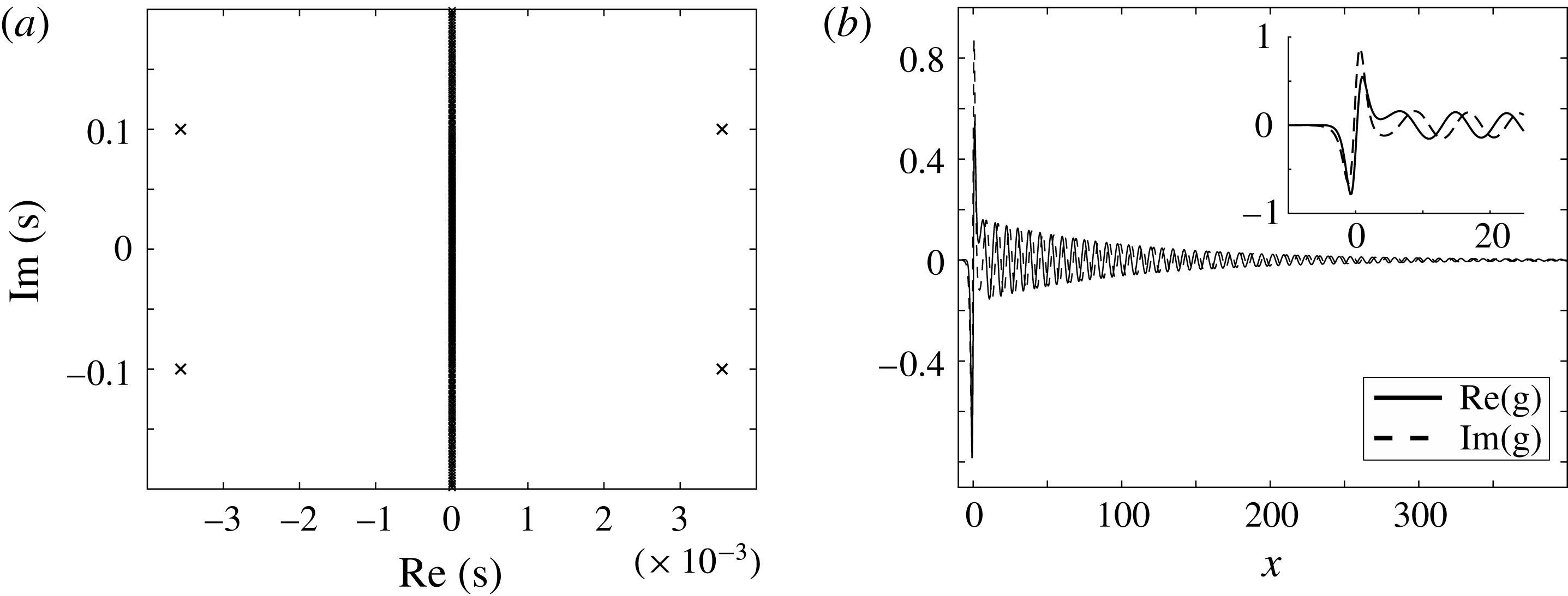
are varied (similar results are found for a typical iia case). Evidently convergence is achieved with a rather large number of discretisation points. The spectrum for this case is shown in figure 6(a). The unstable eigenfunction is shown in figure 6(b). The large
 $x$
behaviour of the eigenfunction is controlled by the balance
 $(1/6)g_{k}^{\prime \prime \prime }\sim sg_{k}$
in (3.4). Therefore the decay is exponential with
 $g_{k}\sim \text{exp}(\unicode[STIX]{x1D707}x)$
as
 $|x|\rightarrow \infty$
, where
 $\unicode[STIX]{x1D707}=(6s)^{1/3}+2\text{i}k\unicode[STIX]{x03C0}/3$
for
 $k=0,1,2$
. For the unstable eigenvalue given in table 1, we obtain the dominant decay rate
 $\unicode[STIX]{x1D707}=0.73-0.41\text{i}$
for
 $x\rightarrow -\infty$
and
 $\unicode[STIX]{x1D707}=-0.01+0.84\text{i}$
as
 $x\rightarrow \infty$
. The latter value indicates a very slow decay downstream requiring a large computational domain. This explains the large value of
 $L$
required to achieve numerical convergence (see table 1).
Type ii solution at
 $a=-0.1357$
,
 $b=0.3$
(
 $\unicode[STIX]{x1D6FC}=226.1$
). Convergence of the eigenvalues in the discrete
 ${\mathcal{M}}$
spectrum computed on a computational domain
 $[-L,L]$
with
 $N$
equally spaced points. One value of
 $s$
in the (
 $s$
,
 $-s$
,
 $s^{\ast }$
,
 $-s^{\ast }$
) quartet is shown for various
 $N$
and
 $L$
(and grid size
 $\text{d}x=2L/N$
).

Stability properties of the type ii solution at
 $a=-0.1357$
,
 $b=0.3$
(
 $\unicode[STIX]{x1D6FC}=226.1$
): (a) Spectrum of the
 ${\mathcal{M}}$
operator and (b) the real and imaginary parts of the unstable eigenfunction for
 $s=0.0036+0.0997\text{i}$
. In (b) the inset shows a close up of the eigenfunction near to the origin.

As noted above, in the case of a neutrally stable steady solution to the present problem, all of the eigenvalues in the spectrum are necessarily located on the imaginary axis. Linear instability remains a possibility, however. For example, it may be the case that there exist non-simple point-spectrum eigenvalues embedded in the continuous spectrum on the imaginary axis which may lead to algebraic growth in time (Holm et al. Reference Holm, Marsden, Ratiu and Weinstein1985). To proceed we adopt an alternative approach suggested by Camassa & Wu (Reference Camassa and Wu1991), Chardard et al. (Reference Chardard, Dias, Nyguyen and Vanden-Broeck2011) and others, which exploits the fact that (3.1) has a Hamiltonian structure. In fact we can write it as
 $$\begin{eqnarray}\unicode[STIX]{x1D702}_{t}=-\frac{1}{6}\frac{\unicode[STIX]{x2202}}{\unicode[STIX]{x2202}x}\left(\frac{\unicode[STIX]{x1D6FF}{\mathcal{H}}}{\unicode[STIX]{x1D6FF}\unicode[STIX]{x1D702}}\right),\quad {\mathcal{H}}(\unicode[STIX]{x1D702},\unicode[STIX]{x1D702}_{x})={\textstyle \frac{1}{2}}\int _{-\infty }^{\infty }\unicode[STIX]{x1D702}_{x}^{2}-3\unicode[STIX]{x1D702}^{3}-6f\unicode[STIX]{x1D702}\hspace{2.22198pt}\text{d}x,\end{eqnarray}$$
where
 ${\mathcal{H}}$
is the Hamiltonian. Consequently a steady solution
 $\unicode[STIX]{x1D702}_{s}$
of (3.1) corresponds to a solution of the equation
 $\unicode[STIX]{x1D6FF}{\mathcal{H}}/\unicode[STIX]{x1D6FF}\unicode[STIX]{x1D702}=0$
. With a general perturbation
 $\unicode[STIX]{x1D701}$
as defined above, i.e. as
 $\unicode[STIX]{x1D702}=\unicode[STIX]{x1D702}_{s}+\unicode[STIX]{x1D716}\unicode[STIX]{x1D701}(x,t)$
, the second variation of
 ${\mathcal{H}}$
at
 $\unicode[STIX]{x1D702}_{s}$
is given by
 $$\begin{eqnarray}\unicode[STIX]{x1D6FF}^{2}{\mathcal{H}}={\textstyle \frac{1}{2}}\int _{-\infty }^{\infty }\unicode[STIX]{x1D701}_{x}^{2}-9\unicode[STIX]{x1D702}_{s}\unicode[STIX]{x1D701}^{2}\,\text{d}x={\textstyle \frac{1}{3}}\langle \unicode[STIX]{x1D701},{\mathcal{K}}\unicode[STIX]{x1D701}\rangle ,\quad \langle f,g\rangle =\int _{-\infty }^{\infty }f\,g^{\ast }\,\text{d}x.\end{eqnarray}$$
If the second variation
 $\unicode[STIX]{x1D6FF}^{2}{\mathcal{H}}$
is positive (or negative) definite then the steady solution
 $\unicode[STIX]{x1D702}_{s}$
is said to be formally stable. Formal stability implies linear stability, although the converse is not necessarily true (see Holm et al.
Reference Holm, Marsden, Ratiu and Weinstein1985). Linear instability can therefore be ruled out if
 $\unicode[STIX]{x1D6FF}^{2}{\mathcal{H}}$
is definite.
Since
 ${\mathcal{K}}$
is a self-adjoint Schrödinger operator, computing its eigenvalue spectrum constitutes a singular Sturm–Louiville problem on the real line (e.g. Titchmarsh Reference Titchmarsh1962; Coddington & Levinson Reference Coddington and Levinson1955) and is a well-studied problem in quantum mechanics and inverse scattering theory (e.g. Landau & Lifshitz Reference Landau and Lifshitz1977; Drazin & Johnson Reference Drazin and Johnson1989). Restricting the admissible perturbations
 $\unicode[STIX]{x1D701}$
to the class of
 $L_{2}(-\infty ,\infty )$
square-integrable functions, we obtain the lower bound (Camassa & Wu Reference Camassa and Wu1991; Keeler Reference Keeler2017),
 $$\begin{eqnarray}\unicode[STIX]{x1D6FF}^{2}{\mathcal{H}}\geqslant {\textstyle \frac{1}{3}}\unicode[STIX]{x1D708}_{0}\langle \unicode[STIX]{x1D701},\unicode[STIX]{x1D701}\rangle .\end{eqnarray}$$
Since
 $\unicode[STIX]{x1D708}_{0}>0$
, we can conclude from (3.8) that
 $\unicode[STIX]{x1D6FF}^{2}{\mathcal{H}}$
is positive definite. This means type i solutions (for the trench and Gaussian dip), which are negative definite, are formally stable and hence linearly stable. For our other solution types,
 $\unicode[STIX]{x1D6FF}^{2}{\mathcal{H}}$
is difficult to calculate analytically and instead we used the numerical pseudo-spectral method to determine the
 ${\mathcal{K}}$
spectrum and, hence, to calculate
 $\unicode[STIX]{x1D708}_{0}$
. (It should be emphasised that if for a given solution it is found that
 $\unicode[STIX]{x1D708}_{0}<0$
, so that the solution is formally unstable, this does not imply that it is linearly unstable and further investigation is needed.) For the type i solutions we confirmed numerically that
 $\unicode[STIX]{x1D708}_{0}>0$
implying linear stability in agreement with the calculations of the
 ${\mathcal{M}}$
spectrum discussed above. For the type ii and iia solutions we found that
 $\unicode[STIX]{x1D708}_{0}<0$
; as we have already discussed, these solutions are found to be unstable when considering the spectrum of the
 ${\mathcal{M}}$
operator.
In the next subsection we perform time-dependent simulations of the unsteady fKdV equation with the goals of confirming the stability properties of the type i and ii solutions, and of following the development of the free surface in each case to large time.
3.2 Time-dependent simulations
We carried out time-dependent simulations of (1.2) on a truncated spatial domain
 $[-L,L]$
, for a specified value of
 $L$
, assuming periodic boundary conditions and using a method similar to that adopted by Chardard et al. (Reference Chardard, Dias, Nyguyen and Vanden-Broeck2011) and Wade et al. (Reference Wade, Binder, Mattner and Denier2014). The method computes spatial derivatives spectrally using a discrete Fourier transform and integrates forward in time using the fourth-order Runge–Kutta algorithm. Further details of the method can be found in (Trefethen Reference Trefethen2000). In numerical practice, we may obtain solutions that satisfy the boundary conditions in the far field by taking
 $L$
sufficiently large. In practice we found that taking
 $\unicode[STIX]{x0394}t\sim 10^{-2}$
and
 $512$
Fourier modes is sufficient to ensure the accuracy of the computations.
Since we assume periodicity in the computations, any disturbance leaving the domain will appear at the opposite end, and such behaviour is clearly unphysical. To prevent this in our computations we introduce a so-called sponge layer (see, for example, Boyd Reference Boyd2000; Alias, Grimshaw & Khusnutdinova Reference Alias, Grimshaw and Khusnutdinova2013; Grimshaw & Maleewong Reference Grimshaw and Maleewong2016) and in fact solve the equation
 $$\begin{eqnarray}\unicode[STIX]{x1D702}_{t}-{\textstyle \frac{3}{2}}\unicode[STIX]{x1D702}\unicode[STIX]{x1D702}_{x}-{\textstyle \frac{1}{6}}\unicode[STIX]{x1D702}_{xxx}+A(x)\unicode[STIX]{x1D702}={\textstyle \frac{1}{2}}\,f_{x},\end{eqnarray}$$
where
 $A(x)=D\{1+\tanh (b_{0}[x-b_{1}])\}$
for positive parameters
 $D$
,
 $b_{0}$
and
 $b_{1}$
. If we choose
 $b_{1}$
to be close to
 $L$
, then
 $A$
is non-zero over a narrow region at the left-hand end of the domain. This has the effect of preventing disturbances leaving the upstream end from entering the downstream end (due to the assumed periodicity) and vice versa.
Multiplying (1.2) by
 $\unicode[STIX]{x1D702}$
and integrating, after making use of (1.3) we obtain
 $$\begin{eqnarray}\frac{\text{d}P}{\text{d}t}=\int _{-\infty }^{\infty }\unicode[STIX]{x1D702}f_{x}\,\text{d}x\equiv W(\unicode[STIX]{x1D702}),\end{eqnarray}$$
where
 $P=\int _{-\infty }^{\infty }\unicode[STIX]{x1D702}^{2}\,\text{d}x$
is the momentum (see Camassa & Wu (Reference Camassa and Wu1991, Appendix C)). The expression
 $W$
is termed the wave resistance coefficient by Camassa & Wu (Reference Camassa and Wu1991) and is interpreted physically as a measure of the power being supplied by the forcing (see also Wu Reference Wu1987). In the absence of forcing,
 $P$
is a conserved quantity. In general
 $P=P(t)$
and so
 $W\neq 0$
; it follows from the integral on the right-hand side of (3.10) that for a topography which is even in
 $x$
, as will be assumed in this paper,
 $\unicode[STIX]{x1D702}(x,t)$
will have a left–right asymmetry about
 $x=0$
. In the presence of forcing it is straightforward to show that the excess mass
 $Q=\int _{-\infty }^{\infty }\unicode[STIX]{x1D702}\,\text{d}x$
is a conserved quantity. The Hamiltonian defined in (3.6) provides a second conserved quantity, corresponding to the energy, and both of these can be used as a check on the fidelity of numerical time-dependent simulations of (1.2). A further check can be made by computing
 $W$
using either of the two alternative expressions given in (3.10) and confirming that the same result is obtained in either case. In the numerical results to be discussed in the next section, both
 $Q$
and
 ${\mathcal{H}}$
were performed in the absence of the sponge layer and it was confirmed that they are conserved.
In the results to be presented below a time-dependent calculation is started using the initial condition
 $\unicode[STIX]{x1D702}(x,0)=\unicode[STIX]{x1D702}_{s}+\unicode[STIX]{x1D716}\hat{\unicode[STIX]{x1D701}}$
where
 $\unicode[STIX]{x1D702}_{s}$
is a chosen steady solution,
 $\hat{\unicode[STIX]{x1D701}}$
is a perturbation and
 $\unicode[STIX]{x1D716}$
is taken to be a small number. In all of the calculations to be presented below we took
 $\unicode[STIX]{x1D716}=0.025$
. If the numerically computed eigenspectrum of the operator
 ${\mathcal{M}}$
revealed a positive largest growth rate, the initial perturbation
 $\hat{\unicode[STIX]{x1D701}}=(g_{k}+g_{k}^{\ast })/2$
, with
 $g_{k}$
the corresponding eigenfunction, was used. Otherwise if the numerically computed spectrum was found to contain only purely imaginary eigenvalues, the initial perturbation
 $\hat{\unicode[STIX]{x1D701}}=\unicode[STIX]{x1D702}_{s}$
was used.
We note that for a given initial condition and a particular choice of the topographic forcing
 $f(x)$
, the solution to the fKdV equation (1.2) is known to be unique (Wu Reference Wu1987). Also, we remark that when presenting unsteady simulations of the fKdV equation for topographic forcing similar to that considered here Wu (Reference Wu1987) and Camassa & Wu (Reference Camassa and Wu1991) both solved the so-called regularised form of the fKdV equation (see Benjamin, Bona & Mahony Reference Benjamin, Bona and Mahony1972), whose equivalence is assured only in the limit of long waves.
We focus on the case of Gaussian topography with
 $f(x)=a\exp (-b^{2}x^{2})$
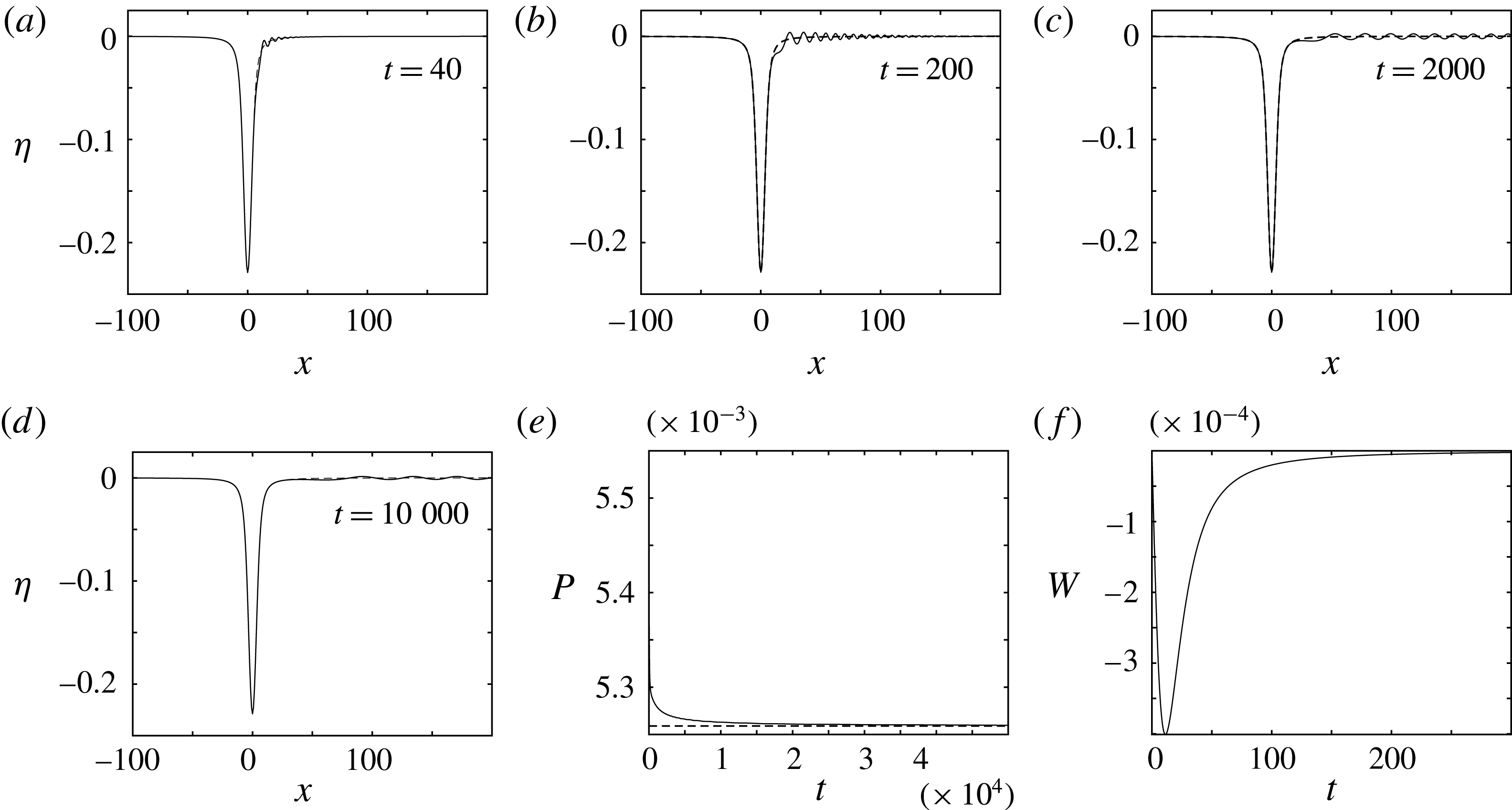
. Our first goal is to confirm the stability results of figure 6. Figure 7 shows the results of a numerical simulation starting from a small perturbation of the unique type i steady solution
 $\unicode[STIX]{x1D702}_{s}$
at
 $\unicode[STIX]{x1D6FC}=141$
(
 $a=-0.085$
,
 $b=0.3$
). The free-surface profile
 $\unicode[STIX]{x1D702}(x,t)$
is shown at different times over a portion of the computational domain
 $[-L,L]$
. We note that the solution in the left side of the domain, which is not shown, remains uniformly zero over the duration of the simulation and that no disturbances are observed to propagate upstream. Also shown in the figure are the time signals of the momentum
 $P$
and the wave resistance coefficient
 $W$
. The initial condition
 $\unicode[STIX]{x1D702}(x,0)=1.025\unicode[STIX]{x1D702}_{s}$
has momentum
 $P(0)=5.53\times 10^{-3}$
which is in excess of the momentum of the steady state type i solution momentum
 $P_{s}=5.26\times 10^{-3}$
. The simulation shows that ultimately the system returns to the steady state
 $\unicode[STIX]{x1D702}_{s}$
as time increases. The wave resistance coefficient
 $W$
approaches zero at large time, which is a necessary condition for the steady state to be recovered. Also
 $W$
is negative during the simulation and so, according to (3.10), the momentum
 $P$
must decrease monotonically. In particular we see that
 $P\rightarrow P_{s}$
as
 $t\rightarrow \infty$
. A
 $\log$
-
 $\log$
plot of the
 $W$
signal indicates that
 $W\sim O(t^{-2})$
for large
 $t$
, and so
 $P$
is expected to approach
 $P_{s}$
algebraically in time; this explains the very long integration time required to recover the steady state.
We emphasise again that momentum cannot be released from the free surface as long as it is symmetric about
 $x=0$
since
 $W$
is zero in this case. Since the initial condition is symmetric, and moreover has a greater momentum than the steady state
 $\unicode[STIX]{x1D702}_{s}$
, it follows that an asymmetric free-surface disturbance must develop in
 $t>0$
if the steady state is to be recovered in the long term. As can be seen in figure 7(a–d), small amplitude waves appear on the leeward side of the free surface. These waves propagate downstream carrying momentum with them. Eventually these waves evanesce and the steady state is recovered. Close inspection of these figures reveals that the free surface, shown with a solid line, overlaps with the steady state
 $\unicode[STIX]{x1D702}_{s}$
, shown with a broken line, over an increasingly wide region as time goes on.
Numerical simulation of (3.9) with Gaussian forcing for
 $\unicode[STIX]{x1D6FC}=141$
, (
 $a=-0.085,b=0.3$
) with
 $L=200$
and
 $N=512$
. The initial condition is
 $\unicode[STIX]{x1D702}(0,t)=1.025\unicode[STIX]{x1D702}_{s}$
, where
 $\unicode[STIX]{x1D702}_{s}$
is the unique type i solution at this
 $\unicode[STIX]{x1D6FC}$
(see figure 3
h). (a–d) Show the solution over a portion of the domain at times
 $t=40$
,
 $200$
,
 $2000$
and
 $10\,000$
. (e,f) Show the momentum
 $P$
and
 $W$
respectively against time. The broken line in (e) is the momentum of the type i steady state,
 $P=5.26\times 10^{-3}$
.

Numerical simulation of (3.9) with Gaussian forcing for
 $\unicode[STIX]{x1D6FC}=226.1$
, (
 $a=-0.1357,b=0.3$
) with
 $L=400$
and
 $N=2048$
(note not all of the domain is displayed). The initial condition is
 $\unicode[STIX]{x1D702}(0,t)=1.025\unicode[STIX]{x1D702}_{s}$
, where
 $\unicode[STIX]{x1D702}_{s}$
is the unique type ii solution at this
 $\unicode[STIX]{x1D6FC}$
(see 3
h). (a–d) Show the solution over a portion of the domain at times
 $t=100$
,
 $t=500$
,
 $t=1000$
,
 $1100$
and
 $1500$
. (f) Shows
 $W$
respectively against time. The dotted curve is the steady solution
 $\unicode[STIX]{x1D702}_{s}$
.

Figure 8 shows the results of a numerical simulation starting from a small perturbation of the type ii steady solutions
 $\unicode[STIX]{x1D702}_{s}$
at
 $\unicode[STIX]{x1D6FC}=226.1$
(
 $a=-0.1357$
,
 $b=0.3$
) respectively. Very similar results are found for a simulation started from a small perturbation of a type iia steady solution. The free-surface profile
 $\unicode[STIX]{x1D702}(x,t)$
is shown at different times over a portion of the computational domain
 $[-L,L]$
. The calculated unstable eigenmode is used as an initial condition for the linearised time-dependent equation (3.2) and excellent agreement is found with the calculated unstable eigenvalue (Keeler Reference Keeler2017). The agreement for the nonlinear time-dependent equation is also good for small times when the initial condition is given by
 $\unicode[STIX]{x1D702}(x,0)=\unicode[STIX]{x1D702}_{s}+1/2\unicode[STIX]{x1D716}(g_{k}+g_{k}^{\ast })$
, with
 $g$
the unstable eigenmode. The initial condition for the calculations in figure 8 is
 $\unicode[STIX]{x1D702}(x,0)=1.025\unicode[STIX]{x1D702}_{s}$
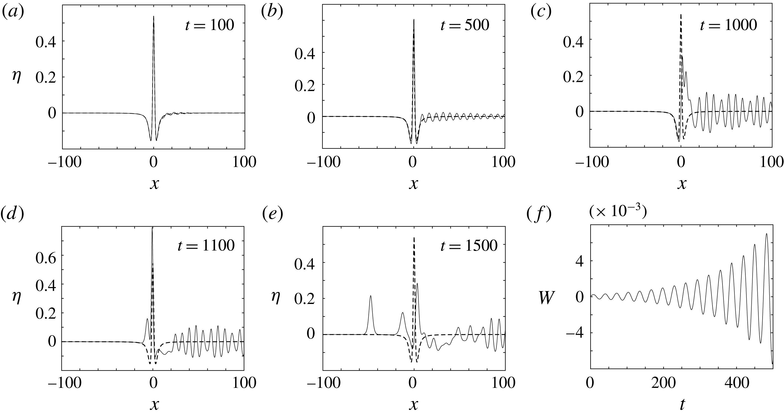
and the different panels show the free-surface profile at different times together with the steady solution, which is shown as a dashed curve. These snapshots show waves travelling downstream in an irregular manner. Additionally, the solution in
 $x<0$
does not remain uniformly zero over the duration of the simulation and after a finite interval soliton-like disturbances emerge and propagate upstream. To conserve
 $Q$
, the excess mass created by these soliton-like disturbances is balanced by a non- uniform depression region which appears directly downstream of the topography. The time signal of the wave resistance coefficient
 $W$
is also shown in the figure and is seen to oscillate with increasing amplitude as time increases. We conclude the solution does not return to the steady state as
 $t$
increases.
We also carried out simulations with the initial condition
 $\unicode[STIX]{x1D702}(x,0)=0$
. Although a stable steady solution exists in this case, this is not approached at large time. Instead unsteady behaviour is observed whose features are in line with those described by Wu (Reference Wu1987), Camassa & Wu (Reference Camassa and Wu1991), Grimshaw & Smyth (Reference Grimshaw and Smyth1986) (see in particular § 6 and figure 11) and Grimshaw, Zhang & Chow (Reference Grimshaw, Zhang and Chow2007).
4 Discussion
We have examined critical free-surface flow over a localised bottom topography using a weakly nonlinear forced Korteweg–de Vries model and by way of numerical solutions of the fully nonlinear problem. Critical flow conditions occur when the Froude number is equal to unity both far upstream and far downstream of the localised topography. In the first part of the paper we considered the steady solutions which are found when the topography takes the form of a Gaussian dip (a simple argument dictates that no steady solutions are possible in the case of a positive–definite topography). For this topography we studied steady solutions via very carefully conducted numerical calculations. The solution space depends on a single parameter,
 $\unicode[STIX]{x1D6FC}$
. For small
 $\unicode[STIX]{x1D6FC}$
there is a unique steady solution, which is negative–definite and which we have termed a type i solution. At a critical value of
 $\unicode[STIX]{x1D6FC}$
a second solution, termed type ii, appears which is not single signed. At larger values of
 $\unicode[STIX]{x1D6FC}$
, further branches of steady solutions appear. In general the steady solutions have algebraic decay in the far field such that the free-surface elevation decays as
 $-(4/3)x^{-2}$
as
 $x\rightarrow \infty$
. Similar algebraic decay can occur for gravity–capillary waves in infinite depth (Akylas, Dias & Grimshaw Reference Akylas, Dias and Grimshaw1998) and for gravity–capillary waves in two-layer flow (Sun Reference Sun1997). To corroborate the numerical solutions, we also constructed asymptotic solutions valid in the limit of small and large
 $\unicode[STIX]{x1D6FC}$
. For large
 $\unicode[STIX]{x1D6FC}$
we successfully constructed an asymptotic solution which captures the negative–definite type i solution as well as the type ii solution. However, an asymptotic description of the apparently infinite sequence of solution branches, types ii a,b,c..., for which an increasing number of ripples are trapped on the free surface around the origin, lies beyond the scope of the present analysis. On this point it is illuminating to highlight the similarity between the presently considered problem and the celebrated Carrier problem discussed at length in, for example, Bender & Orszag (Reference Bender and Orszag1999, p. 464), wherein an increasing number of interior oscillations appear in the solution as the pertinent dimensionless parameter approaches zero. These solutions are not fully captured by a traditional boundary-layer analysis. Determining the asymptotic structure of the type iia,b,c... solutions in the current work is the subject of our current investigations.
Numerical solutions performed using the boundary-integral method and using a conformal mapping technique confirmed the existence of type i, ii and iia solutions in the fully nonlinear regime. However, these solutions do not extend indefinitely to large
 $\unicode[STIX]{x1D6FC}$
. Rather, as
 $\unicode[STIX]{x1D6FC}$
is increased, the free-surface profiles approach a limiting configuration which is locally similar to that found for a classical Stokes wave with an interior angle of
 $120^{\circ }$
at the wave maximum.
In the second part of our investigation, we studied the stability of the steady solutions obtained for a Gaussian dip topography first by computing eigenvalues of the linearised system, and then by numerical computation of the full fKdV initial value problem. For type i solutions all of the eigenvalues were found to lie on the imaginary axis, suggesting linear stability, and this was corroborated by the time-dependent simulations. In fact a simulation initiated with a free surface which is only a small deviation from a type i solution is seen to slowly relax back to this steady state as time increases; the momentum associated with the initial perturbation is leaked downstream in the form of a wavetrain which appears on the downstream side of the free surface shortly after the start of the simulation. The stability calculations for type ii and type iia steady solutions revealed complex eigenvalues which indicate that these solutions are linearly unstable and this was confirmed by time-dependent simulations initiated using the unstable eigenfunction as the form of perturbation. During these simulations, solitary waves are emitted upstream at regular intervals similar to what has been observed by previous workers. Interestingly, a simulation started from a flat free surface does not approach the stable type i solution but instead behaviour somewhat similar to that found by Wu (Reference Wu1987) for critical flow over a positive obstacle is observed: key differences, however, are that the solitary waves which are emitted upstream have different heights and the depression region which appears downstream of the topography is undular rather than flat. The case of a positive topography is well studied (e.g. Grimshaw & Smyth Reference Grimshaw and Smyth1986; Wu Reference Wu1987; Grimshaw et al. Reference Grimshaw, Zhang and Chow2007) and analytic results have been obtained; however, to our knowledge no such results are available for a negative topography.
When reaching our conclusions on the stability properties of the steady solutions for a Gaussian topography/free surface, in addition to numerical eigenvalue calculations and time-dependent simulations, we also applied the Hamiltonian theory of Camassa & Wu (Reference Camassa and Wu1991) to show analytically that negative–definite type i solutions are linearly stable. This was done by demonstrating that the
 ${\mathcal{K}}$
operator has no negative eigenvalues and hence the second variation of the relevant Hamiltonian is positive–definite. Unfortunately for the type ii solutions, which are not single signed, the results of this analysis are inconclusive. Analytic eigenvalue counts which might be used to deduce stability properties in this case have been discussed at some length in the literature. Notably Pelinovsky (Reference Pelinovsky2012) and Kapitula & Stefanov (Reference Kapitula and Stefanov2014) (see also the earlier work by Chugunova & Pelinovsky Reference Chugunova and Pelinovsky2010) independently proved a theorem for linearised systems of the form
 $\unicode[STIX]{x2202}_{x}{\mathcal{L}}u=\unicode[STIX]{x1D706}u$
, which relates the number of potentially unstable eigenvalues
 $\unicode[STIX]{x1D706}$
to the number of negative eigenvalues of the self-adjoint operator
 ${\mathcal{L}}$
. Chardard et al. (Reference Chardard, Dias, Nyguyen and Vanden-Broeck2011) used these ideas to infer stability properties of steady, table-top solitary wave solutions for supercritical flow. Unfortunately, the theorem cannot be applied in the present case of critical flow, since it requires that the essential spectrum of the
 ${\mathcal{L}}$
operator be bounded away from the origin. Here we have
 ${\mathcal{L}}=-{\mathcal{K}}=(1/6)\unicode[STIX]{x2202}_{xx}+(3/2)\unicode[STIX]{x1D702}_{s}$
with essential spectrum
 $[0,\infty )$
, which violates this requirement. We have not been able to identify in the literature an eigenvalue count which applies in this case, and this remains an interesting topic for future work.
Acknowledgement
The work of M.G.B. was supported by the EPSRC under grant EP/K041134/1.
Appendix A. Algebraic decay of a solitary wave for critical flow
In this appendix we demonstrate that a solitary wave solution for critical flow,
 $F=1$
, must decay algebraically in the far field and we determine the leading-order form of this decay. To establish this result we start from the formulation of the problem (2.34)–(2.36). It is convenient then to make a conformal transformation
 $(x,y)\mapsto (\unicode[STIX]{x1D709},\unicode[STIX]{x1D701})$
mapping the physical domain into the infinite strip
 $-H\leqslant \unicode[STIX]{x1D701}\leqslant 0$
in the mapped plane, for some chosen
 $H$
.
Working in a manner similar to that adopted by Choi & Camassa (Reference Choi and Camassa1999) in their discussion of periodic water waves, we write down the problem determining the conformal mapping as
 $$\begin{eqnarray}\displaystyle & \displaystyle y_{\unicode[STIX]{x1D701}\unicode[STIX]{x1D701}}+y_{\unicode[STIX]{x1D709}\unicode[STIX]{x1D709}}=0,\quad \text{in }-H\leqslant \unicode[STIX]{x1D701}\leqslant 0, & \displaystyle\end{eqnarray}$$
 $$\begin{eqnarray}\displaystyle & \displaystyle y=1+s(\unicode[STIX]{x1D709})\quad \text{on }\unicode[STIX]{x1D701}=0, & \displaystyle\end{eqnarray}$$
 $$\begin{eqnarray}\displaystyle & \displaystyle y=b(\unicode[STIX]{x1D709})\quad \text{on }\unicode[STIX]{x1D701}=-H, & \displaystyle\end{eqnarray}$$
where
 $s(\unicode[STIX]{x1D709})=\unicode[STIX]{x1D702}(x(\unicode[STIX]{x1D709}))$
and
 $b(\unicode[STIX]{x1D709})=f(x(\unicode[STIX]{x1D709}))$
describe the free-surface elevation and the bottom topography in the mapped plane respectively. The solution is easily obtained by taking a Fourier transform in
 $\unicode[STIX]{x1D709}$
with wavenumber
 $k$
, and is given by
 $$\begin{eqnarray}y=1+\frac{\unicode[STIX]{x1D701}}{H}+\frac{1}{2\unicode[STIX]{x03C0}}\int _{-\infty }^{\infty }\left({\hat{s}}\,\frac{\sinh (k[\unicode[STIX]{x1D701}+H])}{\sinh (kH)}-\hat{b}\,\frac{\sinh (k\unicode[STIX]{x1D701})}{\sinh (kH)}\right)\text{e}^{\text{i}k\unicode[STIX]{x1D709}}\,\text{d}k,\end{eqnarray}$$
where a hat denotes a transformed variable, and
 $\unicode[STIX]{x1D6FF}(k)$
is the Dirac delta function. Differentiating (A 4) and noting that
 $x_{\unicode[STIX]{x1D709}}=y_{\unicode[STIX]{x1D701}}$
according to the Cauchy–Riemann equations, we find that (see also Viotti, Dutykh & Dias Reference Viotti, Dutykh and Dias2014; Blyth & Părău Reference Blyth and Părău2016)
 $$\begin{eqnarray}x_{\unicode[STIX]{x1D709}}|_{\unicode[STIX]{x1D701}=0}=1/H-T(s_{\unicode[STIX]{x1D709}})+S(b_{\unicode[STIX]{x1D709}}),\end{eqnarray}$$
where
 $T$
and
 $S$
are non-local operators defined by
 $$\begin{eqnarray}T[f(\unicode[STIX]{x1D709})]=\frac{1}{2H}\unicode[STIX]{x2A0D}_{-\infty }^{\infty }f(\unicode[STIX]{x1D709}^{\prime })\coth \left(\frac{\unicode[STIX]{x03C0}}{2H}(\unicode[STIX]{x1D709}^{\prime }-\unicode[STIX]{x1D709})\right)\hspace{2.22198pt}\text{d}\unicode[STIX]{x1D709}^{\prime },\end{eqnarray}$$
and
 $$\begin{eqnarray}S[f(\unicode[STIX]{x1D709})]=\frac{1}{2H}\unicode[STIX]{x2A0D}_{-\infty }^{\infty }f(\unicode[STIX]{x1D709}^{\prime })\tanh \left(\frac{\unicode[STIX]{x03C0}}{2H}(\unicode[STIX]{x1D709}^{\prime }-\unicode[STIX]{x1D709})\right)\hspace{2.22198pt}\text{d}\unicode[STIX]{x1D709}^{\prime }.\end{eqnarray}$$
We formulate the flow problem in the mapped plane in terms of the mapped streamfunction
 $\unicode[STIX]{x1D6F9}(\unicode[STIX]{x1D709},\unicode[STIX]{x1D701})$
, where
 $\unicode[STIX]{x1D6F9}=\unicode[STIX]{x1D713}(x(\unicode[STIX]{x1D709},\unicode[STIX]{x1D701}),y(\unicode[STIX]{x1D709},\unicode[STIX]{x1D701}))$
, and the streamfunction in the physical plane,
 $\unicode[STIX]{x1D713}$
, is defined in the usual way so that
 $u=\unicode[STIX]{x1D713}_{y}$
and
 $v=-\unicode[STIX]{x1D713}_{x}$
. The problem is
 $$\begin{eqnarray}\displaystyle & \displaystyle \unicode[STIX]{x1D6F9}_{\unicode[STIX]{x1D701}\unicode[STIX]{x1D701}}+\unicode[STIX]{x1D6F9}_{\unicode[STIX]{x1D709}\unicode[STIX]{x1D709}}=0,\quad \text{in }-H\leqslant \unicode[STIX]{x1D701}\leqslant 0, & \displaystyle\end{eqnarray}$$
 $$\begin{eqnarray}\displaystyle & \displaystyle \unicode[STIX]{x1D6F9}=1\quad \text{on }\unicode[STIX]{x1D701}=0, & \displaystyle\end{eqnarray}$$
 $$\begin{eqnarray}\displaystyle & \displaystyle \unicode[STIX]{x1D6F9}=0\quad \text{on }\unicode[STIX]{x1D701}=-H, & \displaystyle\end{eqnarray}$$
where we have assumed a unit flux in the streamwise direction in keeping with the non-dimensionalisation introduced in the main part of the paper. The solution is simply
 $\unicode[STIX]{x1D6F9}=\unicode[STIX]{x1D701}/H$
. The Cauchy–Riemann equations immediately yield the relation
 $\unicode[STIX]{x1D6F7}_{\unicode[STIX]{x1D709}}=1/H$
, where
 $\unicode[STIX]{x1D6F7}(\unicode[STIX]{x1D709},\unicode[STIX]{x1D701})$
is the velocity potential in the mapped plane.
At this stage we have satisfied the kinematic conditions on both the bottom topography and on the free surface. The Bernoulli condition on the free surface in the mapped plane demands that
 $$\begin{eqnarray}\frac{F^{2}}{2J}(\unicode[STIX]{x1D6F7}_{\unicode[STIX]{x1D709}}^{2}+\unicode[STIX]{x1D6F9}_{\unicode[STIX]{x1D709}}^{2})+s=\frac{F^{2}}{2},\quad J=x_{\unicode[STIX]{x1D709}}^{2}+y_{\unicode[STIX]{x1D709}}^{2},\end{eqnarray}$$
where all terms are evaluated at
 $\unicode[STIX]{x1D701}=0$
. Taking into account the fact that
 $s(\unicode[STIX]{x1D709})$
is a real function, and considering its Taylor series expansion in Fourier space for both positive and negative values of
 $k$
, we may write down the general small
 $k$
expansion for the surface elevation in Fourier space as
 $$\begin{eqnarray}{\hat{s}}(k)\sim (a_{00}+\text{i}a_{01}\text{sgn}(k))+(a_{10}|k|+\text{i}a_{11}k)+(a_{20}k^{2}+\text{i}a_{21}k|k|)+\cdots \,,\end{eqnarray}$$
where the
 $a_{ij}$
are all real. A similar expansion can be written down for the bottom topography function; since this function is prescribed the precise form of its expansion coefficients are known in advance.
Keeping in mind the application to a Gaussian topographic forcing
 $f(x)$
in the physical plane, as is considered in the main part of the paper, we now assume that
 $b(\unicode[STIX]{x1D709})$
decays at least exponentially as
 $\unicode[STIX]{x1D709}\rightarrow \infty$
. By examining the form of the small
 $k$
expansion of the term in large brackets in the integrand of (A 4), and using (A 5), we find that
 $$\begin{eqnarray}x_{\unicode[STIX]{x1D709}}|_{\unicode[STIX]{x1D701}=0}\sim \frac{1}{H}+\left(\frac{\text{i}a_{01}}{H}\right)\unicode[STIX]{x1D709}^{-1}-\left(\frac{a_{10}}{\unicode[STIX]{x03C0}H}\right)\unicode[STIX]{x1D709}^{-2}+\cdots\end{eqnarray}$$
as
 $\unicode[STIX]{x1D709}\rightarrow \infty$
. The asymptotic form (A 13) has been obtained by making use of Lighthill (Reference Lighthill1958, Theorem 19 on page 52).
Substituting our previous results into the Bernoulli equation (A 11), and considering the limit of large
 $\unicode[STIX]{x1D709}$
, we obtain
 $$\begin{eqnarray}\displaystyle 0 & = & \displaystyle \text{i}a_{01}(1-F^{2})\unicode[STIX]{x1D709}^{-1}+\left[(F^{2}-1)\frac{a_{10}}{\unicode[STIX]{x03C0}}-\frac{3}{2}F^{2}a_{01}^{2}\right]\unicode[STIX]{x1D709}^{-2}\nonumber\\ \displaystyle & & \displaystyle +\,\left[6(1-F^{2})a_{21}+6\text{i}\unicode[STIX]{x03C0}F^{2}a_{01}^{3}-F^{2}(9\text{i}a_{10}-2H^{2})a_{01}\right]\unicode[STIX]{x1D709}^{_{3}}+\cdots\end{eqnarray}$$
as
 $\unicode[STIX]{x1D709}\rightarrow \infty$
. If
 $F\neq 1$
, as is the case for either subcritical flow or for supercritical flow, we are forced to conclude that
 $a_{01}=a_{10}=a_{21}=\cdots =0$
; in this case the decay is known to be exponential, as is discussed by Longuet-Higgins & Fox (Reference Longuet-Higgins and Fox1977), Hunter & Vanden-Broeck (Reference Hunter and Vanden-Broeck1983) and Wade et al. (Reference Wade, Binder, Mattner and Denier2014), for example. If
 $F=1$
, however, it is clear from (A 14) that
 $a_{01}=a_{21}=0$
; moreover at
 $O(\unicode[STIX]{x1D709}^{-4})$
we determine that
 $a_{10}=(4/3)\unicode[STIX]{x03C0}H^{2}$
. Applying Lighthill’s Theorem 19 to (A 12) we conclude that
 $$\begin{eqnarray}s\sim -{\textstyle \frac{4}{3}}(\unicode[STIX]{x1D709}/H)^{-2}+\cdots\end{eqnarray}$$
as
 $\unicode[STIX]{x1D709}\rightarrow \infty$
. We note from (A 13) that
 $x\sim \unicode[STIX]{x1D709}/H+o(\unicode[STIX]{x1D709})$
as
 $\unicode[STIX]{x1D709}\rightarrow \infty$
and hence we find that in the case of critical flow,
 $F=1$
, the free-surface elevation decays algebraically as
 $-(4/3)x^{-2}$
for large
 $x$
. Interestingly, this is precisely the form of the far-field behaviour predicted by the steady fKdV equation (2.3). We note that the same inverse square rate of algebraic decay has been demonstrated for gravity–capillary waves in infinite depth by Akylas et al. (Reference Akylas, Dias and Grimshaw1998), and for gravity–capillary waves in two-layer flow by Sun (Reference Sun1997), who established the decay rate rigorously using analytical methods.