1. Introduction
Falling liquid films, i.e. thin liquid layers flowing down a vertical or inclined wall driven by gravity, are used in various applications such as refrigeration, cooling of heated mechanical or electronic systems, chemical processing (Hu et al. Reference Hu, Yang, Yu and Dai2014), petroleum refineries, desalination (Kouhikamali et al. Reference Kouhikamali, Abadi and Hassani2014) and food processing (Alekseenko, Nakoryakov & Pokusaev Reference Alekseenko, Nakoryakov and Pokusaev1994; Kalliadasis et al. Reference Kalliadasis, Ruyer-Quil, Scheid and Velarde2013), allowing high heat transfer coefficients. The understanding of wave dynamics and the identification of the various phases in the parameter space have a direct impact on the optimization of those processes.
For low film flow rates flowing down a vertical wall, the wave patterns that occur are characterized by small-amplitude waves. The streamlines of those small-amplitude waves are, if drawn in a reference frame moving with the wave celerity
 $c$
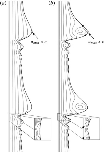
, roughly aligned with the wave profile (see figure 1
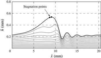
a). Further, the highest (interfacial) velocity is found at the wave crest and is lower than the wave celerity. For higher flow rates, the wave peak height and the maximum surface velocity at the wave crest increase. At a critical flow rate, the maximum surface velocity is equal to the wave celerity, which results in a stagnation point (see Maron, Brauner & Hewitt Reference Maron, Brauner and Hewitt1989), found to be located in the vicinity of the wave crest.
Streamline plot in the frame of reference moving at the wave speed
 $c$
illustrating the characteristics of (a) non-circulating and (b) circulating waves. The maximum speed of the fluid is denoted
 $u_{max}$
. The two insets show (a) the onset of flow separation and (b) flow separation with an open vortex in the fixed frame of reference. The black dots indicate stagnation points.

With a further increase in flow rate, the single stagnation point splits and the two points travel down the wave hump on both sides (see figure 1 b). The region bounded by the two interfacial stagnation points confines a circulating eddy on the interfacial side. Owing to the circulating eddy, these waves are called circulating waves. At the interfacial stagnation point located at the front of the wave, the fluid motion points inwards from the wave hump, which can have a significant influence on the interfacial heat and/or mass transfer. In Islam (Reference Islam2009), for instance, temperature profiles of a falling liquid film are shown and depict the intrusion of a hot finger originating at the stagnation point for a Reynolds number of 50. However, the interpretation of the streamlines in the moving frame of reference, indicating the circulation at the main hump, may also be misunderstood as a trapping of fluid particles (Malamataris & Balakotaiah Reference Malamataris and Balakotaiah2008). For a different illustration of the fluid motion, Malamataris & Balakotaiah (Reference Malamataris and Balakotaiah2008) use pathlines of the fluid particles near the main hump. The pathlines reveal an upwards and downwards movement, in which the streamwise velocity of the fluid particle increases as it moves to the top and decreases as it moves to the bottom.
The identification of circulating eddies in falling films goes back to the work of Davies (Reference Davies1960), who observed that injected tracers in a wavy film flow do not spread laterally. He concluded that streamlines of the flow must depict a closed recirculation zone. However, his physical explanation revealed some deficits, such as for instance the existence of streamlines aligned with the free surface above the recirculation vortex in the moving frame of reference. In Portalski (Reference Portalski1964), a first physical picture of circulating eddies was presented. However, the location of those eddies was found to be in the wave’s trough, for which they cannot be attributed directly to the circulating waves found in the wave hump.
One of the first works showing the possible existence of a stagnation point on the wave’s back is the physical model of Brauner & Maron (Reference Brauner and Maron1983), based on the withdrawal theory. Originally intended to model the substrate thickness that remains after a lump of liquid is flowing over the slow-moving thin substrate, the withdrawal theory also reveals the existence and the position of a stagnation point located on the wave’s back. The ratio between the height of the stagnation point from withdrawal theory,
 $h_{b}$
, and the substrate thickness,
 $h_{s}$
, leads to a threshold for the occurrence of a stagnation point. This threshold was found to be
 $h_{b}/h_{s}=2.72$
. In a later work, Maron et al. (Reference Maron, Brauner and Hewitt1989) estimated this threshold based on numerical simulations, finding the transition from non-circulating to circulating waves to be located between 2.5 and 3.
In Wasden & Dukler (Reference Wasden and Dukler1989), velocity fields inside solitary waves were shown. Although those results were iteratively calculated based on experimental film thickness measurements, they revealed a clear picture of the wave dynamics. Full numerical simulations, including a deformable surface of circulating waves, were published in the late 1990s. Miyara (Reference Miyara2000), for instance, numerically investigated waves of different frequencies, inclinations, Reynolds number and Weber number using the experimental results of Liu & Gollub (Reference Liu and Gollub1994) as a basis for validation. They found that the size of the recirculation zone decreases with decreasing Reynolds number and that the vortex centre moves near the wave crest. For film flows on inclined plates, the amplitude of the main wave hump decreases and the recirculation zone becomes suppressed (for otherwise constant parameters). In Roberts & Chang (Reference Roberts and Chang2000), the recirculation mechanism and the influence of this recirculation on mass transfer is shown together with a criterion for the onset of circulating waves based on a critical wave speed. A detailed comparison and discussion of their findings will be given here in the results section.
In addition to the onset of circulating waves, the onset of flow reversal and flow separation can be seen as distinct characteristics of the instantaneous structure of the flow field in falling films (Malamataris, Vlachogiannis & Bontozoglou Reference Malamataris, Vlachogiannis and Bontozoglou2002; Malamataris & Balakotaiah Reference Malamataris and Balakotaiah2008). The phenomenon of flow separation is shown in the lower insets of figure 1 in the fixed ‘laboratory’ frame of reference. Flow separation is caused by the gradient in surface curvature resulting in a capillary pressure acting in the opposite direction to the flow and thus reducing the velocity beneath the minima of the capillary ripples preceding the main hump of a wave. If the intensity of this force and the time for which it acts are sufficient (starting beneath the first capillary ripple preceding the main hump of a wave), the flow beneath the capillary minima can change direction, leading to a back-flow and consequently to a separation vortex (Dietze, Leefken & Kneer Reference Dietze, Leefken and Kneer2008; Dietze, Al-Sibai & Kneer Reference Dietze, Al-Sibai and Kneer2009). In the inset of figure 1(a), a widening of the streamlines is shown below the wave trough, illustrating a significantly reduced streamwise velocity. The inset of figure 1(b) shows the case with flow separation and a reverse flow between the two cross-stream streamlines, which both end in a stagnation point at the wall.
Besides these flow characteristics discussed above, the transition between the drag–gravity to drag–inertia regimes can be investigated for inclined films. This transition was identified by Ooshida (Reference Ooshida1999) based on the tail structure of solitary waves. The character of the drag–gravity regime is similar to the Nusselt solution for a flat film such that wall-friction drag and gravity are the most dominant effects. Contrarily, the drag–inertia regime is characterized by a steep wave front, where gravity, viscous drag and surface tension balance, and a long tail, where gravity, viscous drag and inertia play a significant role (Kalliadasis et al. Reference Kalliadasis, Ruyer-Quil, Scheid and Velarde2013). Knowledge of this transition is essential for modelling purposes, since Scheid et al. (Reference Scheid, Ruyer-Quil, Thiele, Kabov, Legros and Colinet2005) have shown that the Benney equation properly describes the falling film dynamics in the drag–gravity regime, while the weighted integral boundary layer (WIBL) model is needed in the drag–inertia regime.
In this study, the simplified WIBL model is used to derive criteria for the phase transitions. However, the domain of validity of this model is limited to certain parameter values. As a consequence, we have validated our findings by the full second-order WIBL model, which itself has been validated recently by Chakraborty et al. (Reference Chakraborty, Nguyen, Ruyer-Quil and Bontozoglou2014) by way of direct numerical simulations (DNS). In addition, our own results of fully resolved numerical simulations have been used for validation purpose.
The remainder of this paper is structured as follows. Section 2 provides a description of the numerical methods applied and the criteria used for the onset of circulating waves, flow reversal and flow separation, as well as for the transition from the drag–gravity regime to the drag–inertia regime. Section 3 presents the results for homoclinic orbits and limit cycles, including validation with DNS. Section 4 concludes.
2. Methods
In this section, the WIBL method and its dynamical system for steady travelling waves will be described. Subsequently, criteria for the onset of circulating waves and flow reversal will be presented using self-similar parabolic velocity profiles in terms of the averaged variables, namely film thickness and flow rate. Next, the flow conditions, either on the average film thickness or on the average flow rate, are revealed. Finally, a description of the DNS methodology is given, which is used besides experimental data for a validation of the WIBL model.
2.1. Weighted integral boundary layer model
The WIBL method, whose derivation was first proposed by Ruyer-Quil & Manneville (Reference Ruyer-Quil and Manneville2000) for modelling falling liquid films, consists in reducing a two-dimensional system of conservation equations (for mass and momentum) and the boundary conditions (at the wall and at the free surface) to a one-dimensional model of evolution equations for the local film thickness
 $h$
and the streamwise flow rate
 $q$
. The full second-order model consists of a system of four evolution equations for the unknowns
 $h$
,
 $q$
,
 $s_{1}$
and
 $s_{2}$
, where
 $s_{1}$
and
 $s_{2}$
are at most first-order inertia corrections to the parabolic velocity distribution. The full model is given in appendix A. In this study, most of the results are obtained using a simplified version of the full model, obtained by cancelling the corrections
 $s_{1}$
and
 $s_{2}$
. Alternatively, this ‘simplified’ second-order model can be obtained by integrating the boundary layer equations using the Galerkin method with a parabolic test function. The resulting conservation and momentum equations are
 $$\begin{eqnarray}h_{t}+q_{x}=0\end{eqnarray}$$
and
 $$\begin{eqnarray}\displaystyle {\it\delta}q_{t} & = & \displaystyle \frac{5}{6}h-\frac{5}{2}\frac{q}{h^{2}}-{\it\delta}\frac{17}{7}\frac{q}{h}q_{x}+\left({\it\delta}\frac{9}{7}\frac{q^{2}}{h^{2}}-\frac{5}{6}{\it\zeta}h\right)h_{x}+\frac{5}{6}hh_{xxx}\nonumber\\ \displaystyle & & \displaystyle +\,{\it\eta}\left[4\frac{q}{h^{2}}(h_{x})^{2}-\frac{9}{2h}q_{x}h_{x}-6\frac{q}{h}h_{xx}+\frac{9}{2}q_{xx}\right],\end{eqnarray}$$
where the subscripts indicate the partial derivative with respect to
 $t$
or
 $x$
,
 ${\it\delta}$
denotes the reduced Reynolds number,
 ${\it\zeta}$
the reduced inclination number, and
 ${\it\eta}$
the viscous dissipation number according to Shkadov scaling (Kalliadasis et al.
Reference Kalliadasis, Ruyer-Quil, Scheid and Velarde2013). Note that, for
 ${\it\eta}=0$
, this model reduces to first order in the gradient expansion accounting for the separation of scales inherent to the boundary layer theory. The dimensionless numbers are
 $$\begin{eqnarray}{\it\delta}=\frac{(3\mathit{Re})^{11/9}}{{\it\Gamma}^{1/3}},\quad {\it\zeta}=\frac{\mathit{Ct}(3\mathit{Re})^{2/9}}{{\it\Gamma}^{1/3}}\quad \text{and}\quad {\it\eta}=\frac{(3\mathit{Re})^{4/9}}{{\it\Gamma}^{2/3}}.\end{eqnarray}$$
Therein, the Reynolds, Kapitza and inclination numbers are defined as
 $$\begin{eqnarray}\mathit{Re}=\frac{g\sin {\it\theta}\,\overline{h}^{3}}{3{\it\nu}^{2}},\quad {\it\Gamma}=\frac{{\it\sigma}}{{\it\rho}{\it\nu}^{4/3}(g\sin {\it\theta})^{1/3}}\quad \text{and}\quad \mathit{Ct}=\cot {\it\theta}.\end{eqnarray}$$
The symbol
 $g$
describes the gravitational acceleration,
 $\overline{h}$
the film thickness of the Nusselt flat film solution,
 ${\it\rho}$
the density,
 ${\it\sigma}$
the surface tension,
 ${\it\nu}$
the kinematic viscosity and
 ${\it\theta}$
the inclination angle. Note that the overbar is used for dimensional quantities in the following. The lengths in the streamwise (
 $x$
) and crosswise (
 $y$
) directions scale with
 ${\it\kappa}\overline{h}_{N}$
and
 $\overline{h}_{N}$
, respectively, where
 ${\it\kappa}=1/\sqrt{{\it\eta}}$
is a compression factor for the streamwise coordinate. Further, the time scale is
 ${\it\nu}{\it\kappa}/(g\sin {\it\theta}\,\overline{h}_{N})$
and the velocity scale is
 $g\sin {\it\theta}\,\overline{h}_{N}^{2}/{\it\nu}$
.
For stationary periodic travelling waves moving with the wave celerity
 $c$
, integration of (2.1) with
 $x^{\prime }=x-ct$
gives a relation between the local flow rate
 $q(x^{\prime })$
and the local film thickness
 $h(x^{\prime })$
:
 $$\begin{eqnarray}q(x)=ch(x)+q_{0}.\end{eqnarray}$$
Here the prime has been dropped for the sake of simplicity and
 $q_{0}$
denotes the rate at which the fluid moves under the wave, namely backwards in the moving frame of reference. Integrated over the wavelength
 ${\it\lambda}$
, this equation gives a relation between the average flow rate and the average film thickness:
 $$\begin{eqnarray}\langle q\rangle _{{\it\lambda}}=c\langle h\rangle _{{\it\lambda}}+q_{0}.\end{eqnarray}$$
The system of equations (2.1) and (2.2) can also be rewritten in the moving frame of reference for stationary periodic travelling waves. Replacing the time derivative of the flow rate
 $q_{t}$
with
 $-cq_{x}$
and subsequently all expressions for
 $q$
with an expression for
 $h$
according to (2.5) results in the third-order dynamical system
 $$\begin{eqnarray}h_{xxx}=3\{q_{0}+ch-{\textstyle \frac{1}{3}}h^{3}+{\textstyle \frac{1}{3}}{\it\zeta}h^{3}h_{x}-{\it\delta}N(h,c)h_{x}-{\it\eta}[I(h,c)h_{x}^{2}+J(h,c)h_{xx}]\}/h^{3}\end{eqnarray}$$
with
 $$\begin{eqnarray}\left.\begin{array}{@{}l@{}}N(h,c)={\textstyle \frac{18}{35}}q_{0}^{2}+{\textstyle \frac{2}{35}}cq_{0}h-{\textstyle \frac{2}{35}}c^{2}h^{2},\\ I(h,c)={\textstyle \frac{8}{5}}q_{0}-{\textstyle \frac{1}{5}}ch,\\ J(h,c)=-{\textstyle \frac{3}{5}}ch^{2}-{\textstyle \frac{12}{5}}q_{0}h.\end{array}\right\}\end{eqnarray}$$
This equation is solved by using the continuation and bifurcation tool for ordinary differential equations in the software AUTO-07P (Doedel Reference Doedel2008), and the package HOMCONT for homoclinic solutions.
2.2. Criteria for phase transitions
2.2.1. Onset of circulating waves
Non-circulating waves are characterized by a wave celerity that is higher than the maximal surface velocity of the wave, while it is opposite for circulating waves, as illustrated in figure 1. Thus, for the onset of circulating waves, the maximal velocity of the wave,
 $u_{max}$
, has to be equal to the wave celerity. The velocity profile neglecting first-order corrections is parabolic and given by
 $$\begin{eqnarray}u(y,x,t)=3\frac{q(x,t)}{h(x,t)}\left(\frac{y}{h(x,t)}-\frac{1}{2}\left(\frac{y}{h(x,t)}\right)^{2}\right),\end{eqnarray}$$
with the maximum velocity found at the interface for
 $y=h(x,y)$
. Malamataris & Balakotaiah (Reference Malamataris and Balakotaiah2008) have shown by numerical simulations that the velocity in the region of the wave crest is well described by a parabolic profile. Substituting the local flow rate by (2.5) leads to the maximal surface velocity
 $$\begin{eqnarray}u_{max}=\frac{3}{2}\left(c+\frac{q_{0}}{h_{max}}\right).\end{eqnarray}$$
Note that
 $q_{0}$
represents the flow rate in the moving frame of reference and is always negative. Consequently, the maximum surface velocity is found when
 $q_{0}/h$
is minimum, i.e. for
 $h=h_{max}$
. Comparing the surface velocity to the wave celerity yields the condition for the onset of circulating waves:
 $$\begin{eqnarray}c_{circ}+3\frac{q_{0}}{h_{max}}=0.\end{eqnarray}$$
The same criterion is derived by Malamataris & Balakotaiah (Reference Malamataris and Balakotaiah2008) using the stream function in a moving frame of reference, setting the gradient with respect to the crosswise coordinate to zero at the position
 $y=h_{max}$
. The condition can be transformed, if
 $q_{0}$
is replaced by using (2.6), to
 $$\begin{eqnarray}c_{circ}=\frac{3\langle q\rangle _{{\it\lambda}}}{3\langle h\rangle _{{\it\lambda}}-h_{max}}.\end{eqnarray}$$
This expression for the critical wave speed is different from the value of
 $\bar{c}=g\bar{h}_{max}^{2}/2{\it\nu}$
(or in dimensionless form
 $c_{circ}=2h_{max}^{2}$
) proposed by Roberts & Chang (Reference Roberts and Chang2000), which was obtained from the Nusselt velocity profile
 $$\begin{eqnarray}\bar{u}(y,x,t)=\frac{g}{{\it\nu}}\left(\overline{y}\,\bar{h}-\frac{\bar{y}^{2}}{2}\right),\quad \text{with }\bar{y}=\bar{h}=\bar{h}_{max},\end{eqnarray}$$
using the flat film solution between the local flow rate and the local film thickness, i.e.
 $q=h^{3}/3$
.
2.2.2. Onset of flow reversal
The onset of flow reversal can be attributed either to a vanishing local flow rate
 $q=0$
(equal to a zero net flux) or to a surface velocity of zero, both in the fixed frame of reference. Equation (2.5) allows again for a critical wave celerity
 $$\begin{eqnarray}c_{rev}=-\frac{q_{0}}{h_{min}},\end{eqnarray}$$
or if
 $q_{0}$
is replaced by using (2.6)
 $$\begin{eqnarray}c_{rev}=\frac{\langle q\rangle _{{\it\lambda}}}{\langle h\rangle _{{\it\lambda}}-h_{min}}.\end{eqnarray}$$
2.2.3. Onset of flow separation
The onset of flow reversal in the vicinity of the wave trough is closely related to the occurrence of flow separation. In the case of flow separation, a separation vortex is formed at the wall, leading to a counter-current flow in the near-wall region. Above this vortex, the flow can still travel in the direction of the main flow. The onset of flow separation is thus associated with a locally vanishing wall shear stress
 $$\begin{eqnarray}{\it\tau}_{W}(x)=\left.\frac{\partial u}{\partial y}\right|_{y=0}=0.\end{eqnarray}$$
This transition criterion becomes at leading order
 $$\begin{eqnarray}{\it\tau}_{W}(x)=3\frac{q}{h^{2}}=0,\end{eqnarray}$$
which coincides with the approximation given by Malamataris & Balakotaiah (Reference Malamataris and Balakotaiah2008). We see that at leading order, the criterion for flow separation coincides with that for flow reversal, i.e.
 $q=0$
. However, with first-order corrections, the onset of flow separation also becomes dependent on the spatial derivatives of the flow rate and the film thickness (see (B 3) in appendix B).
2.2.4. Transition drag–gravity to drag–inertia
Using a regularized long-wave evolution equation for the film thickness, Ooshida (Reference Ooshida1999) identified two different wave regimes: (i) one at small Reynolds number dominated by the balance between viscous and gravity forces, the exact balance of which gives the Nusselt flat film solution, and referred to as the ‘drag–gravity’ regime, and (ii) one at larger Reynolds number for which inertia forces become important, and referred to as the ‘drag–inertia’ regime. Ooshida found that the tail length decreases (or increases) for increasing Reynolds number in the drag–gravity (drag–inertia) regime, the transition between the two regimes then being at the smallest tail length. Kalliadasis et al. (Reference Kalliadasis, Ruyer-Quil, Scheid and Velarde2013) have reproduced Ooshida’s results using the WIBL model for vertical plates.
Having in mind that the tail length behaviour versus Reynolds number allows one to identify the transition between the drag–gravity and drag–inertia regimes, namely when there is a minimum, we track this transition for various inclinations. The length of the wave tail is computed by writing the eigenvalue problem from the dynamical system (2.7), namely substituting
 $h=1+\text{e}^{{\it\lambda}x}$
, where
 ${\it\lambda}$
is the eigenvalue, and linearizing around
 $h=1$
. The obtained characteristic equation is
 $$\begin{eqnarray}{\it\lambda}^{3}+{\it\lambda}^{2}{\it\eta}\left(-\frac{12}{5}+\frac{27}{5}c\right)+{\it\lambda}\left\{{\it\delta}\left(\frac{6}{5}c^{2}-\frac{34}{35}c+\frac{6}{35}\right)-{\it\zeta}\right\}-3(c-1)=0,\end{eqnarray}$$
and gives one real solution, denoted
 ${\it\lambda}_{r}$
, and two complex conjugates. Following Ooshida (Reference Ooshida1999), the tail length of a wave is proportional to
 $1/{\it\lambda}_{r}$
and can be determined using the calculated data of
 $c$
versus
 ${\it\delta}$
for a fixed
 ${\it\zeta}$
as later provided in figure 2(c).
2.3. Flow conditions
To solve the dynamical system (2.7), one additional constraint, either on the flow rate or on the average film thickness, is needed. Both constraints will be applied in this study. A fixed flow rate, denoted as open flow condition (Scheid et al.
Reference Scheid, Ruyer-Quil, Thiele, Kabov, Legros and Colinet2005), describes the flow behaviour under experimental conditions in which a periodically modulated flow rate is imposed at the inlet, provided the wave has not experienced any secondary instability (subharmonic), breaking the initial forcing period. Thus for stationary periodic waves, the time-averaged flow rate over one period in a fixed reference frame (or equivalently the spatially averaged flow rate over one wavelength,
 ${\it\lambda}$
, in a moving reference frame) remains constant, which changes (2.2) and (2.6) to
 $$\begin{eqnarray}\langle q\rangle _{{\it\lambda}}=\frac{1}{3}\quad \text{and}\quad \langle h\rangle _{{\it\lambda}}=\frac{1/3-q_{0}}{c}.\end{eqnarray}$$
The second possible constraint is a fixed amount of liquid enclosed in the spatial period,
 ${\it\lambda}$
, also denoted as closed flow condition (Scheid et al.
Reference Scheid, Ruyer-Quil, Thiele, Kabov, Legros and Colinet2005). This constraint is equivalent to periodic boundary conditions, which are often used in numerical studies and will also be used later in the direct numerical approach. The fixed volume of liquid enclosed yields a constant average film thickness and thus
 $$\begin{eqnarray}\langle h\rangle _{{\it\lambda}}=1\quad \text{and}\quad \langle q\rangle _{{\it\lambda}}=q_{0}+c.\end{eqnarray}$$
Note that
 $q_{0}$
can be parametrized with the substrate film thickness,
 $h_{s}$
, which is the thickness of the flat film region surrounding a wave. For a flat film, (2.2) gives
 $q=h_{s}^{3}/3$
. Together with (2.5), this then gives
 $$\begin{eqnarray}q_{0}=\frac{h_{s}^{3}}{3}-ch_{s},\end{eqnarray}$$
which will be used for computing homoclinic solutions by setting
 $h_{s}$
to unity. Now, with the closed flow condition, the volume of liquid enclosed corresponds for a given Reynolds number to the liquid enclosed in the flat film solution
 ${\it\lambda}\overline{h}_{N}$
(in the dimensional form). Thus, the Reynolds number (denoted as
 $\mathit{Re}_{\overline{h}_{N}}$
or equivalently in Shkadov scaling
 ${\it\delta}_{\overline{h}_{N}}$
) is directly tied to the average film thickness. On the contrary, for the open flow condition, corresponding to a fixed Reynolds number, the average film thickness is adjusted. Thus, this Reynolds number is directly tied to the (time-) average flow rate, denoted as
 $\mathit{Re}_{\overline{q}}$
or equivalently
 ${\it\delta}_{\overline{q}}$
. A direct transformation between the two different Reynolds numbers is not possible, except for a flat film, for which they coincide. However, the flow rate-based Reynolds number for the closed flow condition can be calculated based on the flow field obtained. A comparison of the periodic travelling waves obtained for the closed and open flow conditions using either the flow rate-based Reynolds number or the film thickness-based Reynolds number reveals identity of the two solutions.
2.4. Fully resolved two-phase modelling using the volume of fluid approach
The free-surface flow of two immiscible and incompressible fluids is numerically calculated by solving the fully resolved Navier–Stokes equations for mass,
 $$\begin{eqnarray}\frac{\partial {\it\rho}}{\partial t}+\frac{\partial {\it\rho}u_{i}}{\partial x_{i}}=0,\end{eqnarray}$$
and momentum,
 $$\begin{eqnarray}\frac{\partial {\it\rho}u_{i}}{\partial t}+u_{j}\frac{\partial {\it\rho}u_{i}}{\partial x_{j}}=-\frac{\partial p}{\partial x_{i}}+{\it\eta}\frac{\partial ^{2}{\it\rho}u_{i}}{\partial x_{j}\partial x_{j}},\end{eqnarray}$$
combined with the volume of fluid (VOF) method (see Hirt & Nichols Reference Hirt and Nichols1981) using the Open Field Operation and Manipulation library (OpenFOAM; see Jasak Reference Jasak1996; Ubbink Reference Ubbink1997; Rusche Reference Rusche2002). The VOF approach has often been used in the field of falling liquid films, such as for example in Gao, Morley & Dhir (Reference Gao, Morley and Dhir2003), Dietze (Reference Dietze2010), Doro & Aidun (Reference Doro and Aidun2013), Albert, Marschall & Bothe (Reference Albert, Marschall and Bothe2014) and Dietze et al. (Reference Dietze, Rohlfs, Nährich, Kneer and Scheid2014).
In the VOF approach, a scalar transport equation for the volume fraction
 ${\it\alpha}$
is introduced
 $$\begin{eqnarray}\frac{\partial {\it\alpha}}{\partial t}+\frac{\partial (u_{i}{\it\alpha})}{\partial x_{i}}=0.\end{eqnarray}$$
Similar to the works of Dietze (Reference Dietze2010) and Doro & Aidun (Reference Doro and Aidun2013), an interface compression scheme (see also Rusche Reference Rusche2002) of the form
 $$\begin{eqnarray}\frac{\partial {\it\alpha}}{\partial t}+\frac{\partial u_{i}{\it\alpha}}{\partial x_{i}}+\frac{\partial u_{i,r}{\it\alpha}(1-{\it\alpha})}{\partial x_{i}}=0,\end{eqnarray}$$
where
 $u_{i,r}$
is an artificial ‘compression velocity’, is used to counteract interface smearing by numerical diffusion. The surface tension force,
 $f_{i}^{{\it\sigma}}$
, is calculated by the continuum surface tension model (see Brackbill, Kothe & Zemach Reference Brackbill, Kothe and Zemach1992):
 $$\begin{eqnarray}f_{i}^{{\it\sigma}}={\it\sigma}{\it\kappa}=-{\it\sigma}\boldsymbol{n}(\boldsymbol{{\rm\nabla}}\boldsymbol{\cdot }\boldsymbol{n}).\end{eqnarray}$$
A possible way to calculate the surface curvature
 ${\it\kappa}$
(also implemented in the original interFoam solver) is to determine the second derivative of the volume fraction field
 ${\it\alpha}$
, which yields
 $$\begin{eqnarray}{\it\kappa}=\frac{\boldsymbol{{\rm\nabla}}{\it\alpha}}{\left|\boldsymbol{{\rm\nabla}}{\it\alpha}\right|}(\boldsymbol{{\rm\nabla}}{\it\alpha}).\end{eqnarray}$$
However, this second derivative can lead to strong non-physical oscillations (parasitic currents) on the wave, even for small interfacial smearing. In order to increase the accuracy of the calculation of the surface tension force, we introduce a height function (see also Binz, Rohlfs & Kneer Reference Binz, Rohlfs and Kneer2014; Rohlfs, Binz & Kneer Reference Rohlfs, Binz and Kneer2014), on the basis of which the surface curvature is calculated. Therein, the height of the fluid layer, i.e. the film thickness, is determined by a local integration of the volume fraction
 ${\it\alpha}$
in crosswise direction from the wall to the upper boundary. Note that the fixed orientation of the integration is valid only if the main orientation of the surface normal is in the crosswise direction, which is true for the waves examined and consistent with small spatial and temporal modulation of the interface.
Based on the distribution of the film thickness,
 $h(x)$
, the local curvature is calculated by
 $$\begin{eqnarray}{\it\kappa}=\frac{h_{xx}}{(1+h_{x}^{2})^{3/2}}.\end{eqnarray}$$
The fluid properties are obtained through volume averaging of the respective phase properties, i.e.
 $$\begin{eqnarray}{\it\rho}={\it\alpha}{\it\rho}_{1}+(1-{\it\alpha}){\it\rho}_{2}\quad \text{and}\quad {\it\mu}={\it\alpha}{\it\mu}_{1}+(1-{\it\alpha}){\it\mu}_{2}.\end{eqnarray}$$
For the spatial discretization of the two-dimensional domain, hexagonal cells with a uniform cell size in the streamwise and crosswise directions have been chosen according to previous work of Dietze et al. (Reference Dietze, Rohlfs, Nährich, Kneer and Scheid2014). The spatial and temporal resolution has been identified for each flow condition examined by a rigorous mesh independence analysis. For the temporal discretization, a uniform time-step size has been applied. The second-order central differences scheme is used for all spatial discretization and a first-order bounded implicit scheme is chosen for temporal discretization (Rusche Reference Rusche2002).
3. Results
The results presented in this section are divided into two parts. First, the onset of circulating waves is studied for the homoclinic waves by using the WIBL model. In addition, the onset of circulating waves is compared to the transition from the drag–gravity to the drag–inertia regime and to the onsets of flow separation and flow reversal. In the second part, waves of finite wavelength, or respectively finite frequency, are analysed using the DNS and WIBL approaches. Additionally, comparisons to experimental results are provided in this part.
Although a complete ‘zoology’ of waves exist in falling films, such as hole waves (
 ${\it\gamma}_{1}$
type wave) or hump waves (
 ${\it\gamma}_{2}$
type wave) – see Chang & Demekhin (Reference Chang, Demekhin, Möbius and Miller2002) – as well as one- or multiple-hump waves, we only focus in this work on one-hump waves, as they have the largest amplitude and are thus primarily subject to the occurrence of recirculation eddies.
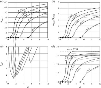
(a) Maximum film thickness, (b) ratio between maximum and minimum film thickness, (c) wave tail length and (d) wave speed as functions of the reduced Reynolds number
 ${\it\delta}$
for
 ${\it\eta}=0.1$
. The grey lines and symbols correspond to the full second-order model, whereas the black ones correspond to the simplified model. The stars indicate the onset of circulating waves, the crosses the onset of flow reversal, the open circles the transition between drag–gravity and drag–inertia regimes, and the filled circles the onset of waves.

3.1. Homoclinic orbits
The basic characteristics, i.e. wave peak height and wave speed, of one-hump homoclinic solutions (
 ${\it\gamma}_{2}$
type waves; Chang & Demekhin Reference Chang, Demekhin, Möbius and Miller2002) as a function of the reduced Reynolds number
 ${\it\delta}$
and the inclination number
 ${\it\zeta}$
are shown in figure 2 using the full second-order model (grey lines) and the simplified second-order model (black lines). The filled circles indicate the border with the stable flat film solution, i.e. for
 ${\it\delta}<5/2{\it\zeta}$
. Stars and crosses are placed at the position of transition to circulating waves and transition to flow reversal, respectively, in accordance with the criteria (2.12) and (2.15) for the critical wave celerity, which simplify for homoclinic orbits, taking
 $h_{s}=1$
, and thus with
 $\langle q\rangle _{{\it\lambda}}=1/3$
and
 $\langle h\rangle _{{\it\lambda}}=1$
, to
 $$\begin{eqnarray}c_{circ}=-\frac{1}{h_{max}-3}\end{eqnarray}$$
and
 $$\begin{eqnarray}c_{rev}=\frac{1}{3(1-h_{min})}.\end{eqnarray}$$
Note that the closed and open flow conditions coincide for homoclinic solutions. Furthermore, the transition between the drag–gravity and drag–inertia regimes is illustrated by the open circles, whereby the transition is taken at the position where the tail length is minimal (see figure 2 c), as explained earlier. Because this transition occurs for low-amplitude waves, for which Scheid et al. (Reference Scheid, Ruyer-Quil, Thiele, Kabov, Legros and Colinet2005) have shown that the Benney equation is valid, no significant difference between the simplified model and the full second-order model is expected.
Figure 2(a) shows the maximum film thickness, revealing a rather constant value
 $h_{max}\approx 2.5$
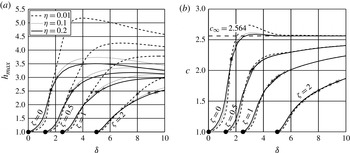
for the transition to circulating waves (stars), despite the model used. An additional variation of the viscous dissipation number (
 $0.01\leqslant {\it\eta}\leqslant 0.2$
) confirms this threshold value (see figure 3
a). Beyond the onset of circulating waves, the solution of the two models diverges significantly. Owing to the fixed substrate film thickness in the homoclinic solution that we fixed to unity, the plot for
 $h_{max}$
is equal to the plot for
 $h_{max}/h_{s}$
. For modelling the wavy flow in inclined thin films, Brauner & Maron (Reference Brauner and Maron1983) apply the withdrawal theory in order to estimate the substrate thickness as well as the location of a stagnation point at the rear interface. The ratio between this location and the substrate thickness is found to take a constant value of 2.72, which they associate with a critical ratio for the onset of circulating waves. This value agrees reasonably with our simulation results of 2.5 and with the value proposed by Maron et al. (Reference Maron, Brauner and Hewitt1989) based on numerical simulations (
 $h_{max}/h_{s}\in [2.5{-}3]$
). Using the minimum film thickness, found in the wave’s trough, as an evaluation criterion reveals for the ratio
 $h_{max}/h_{min}$
a value slightly above 3.
Influence of viscous dissipation number: (a) maximum film thickness and (b) wave speed as functions of the reduced Reynolds number
 ${\it\delta}$
for
 ${\it\eta}=0.01$
,
 ${\it\eta}=0.1$
and
 ${\it\eta}=0.2$
using the full second-order model. The stars indicate the onset of circulating waves and the crosses the onset of flow reversal.

The maximum film thickness at the onset of flow reversal is illustrated by the crosses in figure 2(a). This threshold value decreases from 2.4 for
 ${\it\zeta}=0$
to 2.15 for
 ${\it\zeta}=2$
. In contrast to the onset of circulating waves, figure 3 shows a significant influence of the viscous dissipation number on the onset of flow reversal. The simulation results reveal that the onset of flow reversal can be either below the onset of circulating waves (for lower values of
 ${\it\eta}$
) or above (for higher values of
 ${\it\eta}$
). Note that high values of
 ${\it\eta}$
correspond to low values of the Kapitza number, and thus a reduced surface tension, resulting in less intense capillary ripples.
The wave’s propagation speed is presented in figure 2(d). According to Ruyer-Quil & Manneville (Reference Ruyer-Quil and Manneville2005), the wave speed reaches a constant value of
 $c_{\infty }=2.738$
as
 ${\it\delta}\rightarrow \infty$
using the simplified second-order model and
 $c_{\infty }=2.564$
using the full second-order model. Recently, Chakraborty et al. (Reference Chakraborty, Nguyen, Ruyer-Quil and Bontozoglou2014) have shown by DNS an asymptotic value of
 $c_{\infty }=2.560$
, and have more generally validated the full second-order model in a wide parameter range, including the one covered by the present work. As shown in figure 2(d), the difference in the wave speed of the two models is rather small at the onset of circulating waves, but diverges thereafter. The wave speed at the onset of circulating waves shows a significant decrease with the inclination number
 ${\it\zeta}$
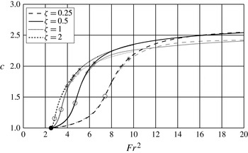
. A different representation of the wave speed dependence on the two parameters, i.e. the reduced Reynolds number and the inclination number, is through the square of the Froude number,
 $\mathit{Fr}^{2}={\it\delta}/{\it\zeta}$
, which compares the speed of the ‘kinematic wave’ and the speed of the ‘surface gravity wave’ (Kalliadasis et al.
Reference Kalliadasis, Ruyer-Quil, Scheid and Velarde2013). In terms of this number, the critical threshold for the long-wave instability is
 $\mathit{Fr}^{2}=5/2$
. Figure 4 shows the dependence of the wave speed on the square of the Froude number obtained with the full second-order and the simplified model. The results of the two models agree well before the onset of flow reversal. For
 $\mathit{Fr}\rightarrow \infty$
the curves (representing different values of
 ${\it\zeta}$
) converge due to the presence of an asymptote for the phase speed for large values of
 ${\it\delta}$
(Chakraborty et al.
Reference Chakraborty, Nguyen, Ruyer-Quil and Bontozoglou2014). This convergence is found to occur earlier for larger values of
 ${\it\zeta}$
. Note that the curves for
 ${\it\zeta}=1$
and
 ${\it\zeta}=2$
overlap very well even before the onset of circulating waves. Nevertheless, the threshold value for the various ‘phases’ in terms of
 $c$
and
 $\mathit{Fr}^{2}$
for the onsets are significantly different.
Wave speed as a function of the Froude number (
 $\mathit{Fr}^{2}={\it\delta}/{\it\zeta}$
) for
 ${\it\eta}=0.1$
. For the symbol legend, see caption of figure 2. The graph shows the divergence of the results of the full second-order model (grey lines) and the simplified model (black lines) near the onset of flow reversal.

The onset of circulating waves for one-hump homoclinic solutions as a function of the reduced Reynolds number
 ${\it\delta}$
and the reduced inclination number
 ${\it\zeta}$
for various values of the streamwise viscous dissipation number
 ${\it\eta}$
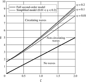
is calculated based on the criterion (3.1) and depicted in figure 5. The diagram shows the borders of three different phases: no waves, non-circulating waves and circulating waves.
Transition from non-circulating to circulating waves for homoclinic solutions: dependence on the dissipation number
 ${\it\eta}$
.

Onset of flow reversal for homoclinic solutions: dependence on the dissipation number
 ${\it\eta}$
.

For low values of
 ${\it\delta}$
, i.e.
 ${\it\delta}\leqslant 5/2{\it\zeta}$
(or
 $\mathit{Fr}^{2}\leqslant 5/2$
), a stable flat film solution exists. Above this threshold, the film is unstable against infinitesimal long-wave disturbances such that sinusoidal waves develop on the film surface. The film surface velocity is always lower than the wave propagation velocity, such that these waves are of non-circulating wave type. The upper three threshold lines mark the onset of circulating waves for different values of the viscous dispersion number
 ${\it\eta}$
. Using the simplified second-order model, only a minor influence of the viscous dispersion number on the threshold value is found. In contrast, the threshold value increases with the dispersion number for higher values of
 ${\it\zeta}$
if the full second-order model is applied. For the vertical case (
 ${\it\zeta}=0$
), the threshold value for all values of
 ${\it\eta}$
and both models is
 ${\it\delta}=1.65\pm 0.025$
.
Using the data obtained from the full second-order model yields the following correlation for the onset of circulating waves,
 $$\begin{eqnarray}{\it\delta}_{circ}\approx -1.28+(2+{\it\zeta})^{0.46{\it\eta}+1.6},\end{eqnarray}$$
which fits the numerical data with
 $R^{2}=0.995$
for
 $0.01\leqslant {\it\eta}\leqslant 0.2$
. (The coefficient of determination,
 $R^{2}$
, is defined as
 $1-(SSE/SST)$
, where
 $SSE$
denotes the sum of squared error and
 $SST$
the sum of squared total.)
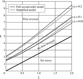
Figure 6 shows the onset of flow reversal based on criterion (3.2). Both models reveal a strong dependence of the onset on the inclination number and a less strong influence on viscous dissipation. However, compared to the onset of circulating waves, the onset of flow reversal is more significantly influenced by viscous dissipation. The difference in the results obtained with the two models is found to increase with inclination number. With the obtained data from the full second-order model, the following correlation for the onset of flow reversal is obtained:
 $$\begin{eqnarray}{\it\delta}_{rev}\approx -1.28+(2+{\it\zeta})^{1.2{\it\eta}+1.5},\end{eqnarray}$$
which fits the numerical data with
 $R^{2}=0.995$
for
 $0.01\leqslant {\it\eta}\leqslant 0.2$
.
Similarly to the circulating wave transition, the onset of the transition between the drag–gravity and the drag–inertia regimes has been found to be independent of the viscous dissipation parameter
 ${\it\eta}$
using the simplified model (not shown).
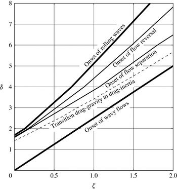
Figure 7 illustrates how the onset of circulating waves is located in the phase diagram compared to the transition between the drag–gravity and drag–inertia regimes for
 ${\it\eta}=0.1$
. The simulation results reveal that this transition occurs before the onset of circulating waves, which agrees with the fact that the flow field of circulating waves differs significantly from the Nusselt flat film solution. The width of the drag–inertia regime without circulating waves increases with the inclination number
 ${\it\zeta}$
, which suggests that strong deviations from the Nusselt flat film solution are necessary at the onset of circulating waves for inclined films.
Phase diagram for one-hump homoclinic solutions with
 ${\it\eta}=0.1$
. Drawn by simulation results obtained from the simplified WIBL model.

The onset of flow separation also depicted in figure 7 is not calculated by the continuation solver directly, but in a post-processing step for a large number of solutions with different values of
 ${\it\zeta}$
based on the first-order approximation of the wall shear stress, estimated by (B 3) in appendix B. The onset of flow separation is consequently associated with the vanishing of the absolute minimum wall shear stress, denoted
 $|\!\min ({\it\tau}_{W})|$
. For validation, the streamline plots in the vicinity of the transition region have been revealed, showing that the onset of flow separation occurs in this area. For
 ${\it\eta}=0.1$
, the onset of flow separation is found to occur for smaller values of the Reynolds number than the onset of circulating waves. Again, the width of the flow separation regime without circulating waves increases with the inclination number
 ${\it\zeta}$
.
Besides the onset of flow separation, the onset of flow reversal is calculated based on the criterion (3.2). Figure 7 shows a significant difference between the onset of flow separation and the onset of flow reversal for larger inclination numbers. This reveals the existence of a small vortex at the wall, slowly growing with an increase in Reynolds number. A further discussion on the onset of flow separation and flow reversal is given later for the limit cycles.
3.2. Limit cycles
The homoclinic orbits in the previous section describe solitary wave solutions of infinite wavelength. For naturally developing waves or for a monochromatic excitation, however, waves of finite length develop. Owing to the additional degree of freedom, an additional independent parameter (the wave frequency or the wavelength) arises together with the reduced Reynolds number and the reduced inclination number.
3.2.1. Validation by experimental and direct numerical comparison for vertical plates
To compare the results of the WIBL model with data from experiments and DNS, parameters have been chosen according to the experimental conditions investigated in Dietze (Reference Dietze2010). Using dimethyl sulfoxide (DMSO) as a working fluid in a vertically inclined cylinder of large radius, the values for the viscosity, density and surface tension are
 ${\it\nu}=2.85\times 10^{-6}~\text{m}^{2}~\text{s}^{-1}$
,
 ${\it\rho}=1098.3~\text{kg}~\text{m}^{-3}$
and
 ${\it\sigma}=0.0484~\text{N}~\text{m}^{-1}$
, respectively. From the various flow conditions presented in that work, a case that is characterized by no circulating waves (
 $\mathit{Re}_{\overline{q}}=6.8$
and
 $\bar{f}=24~\text{Hz}$
) and a case that is characterized by the presence of circulating waves (
 $\mathit{Re}_{\overline{q}}=15$
and
 $\bar{f}=16~\text{Hz}$
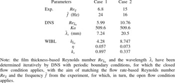
) have been chosen. The values of the dimensional and dimensionless parameters (in Reynolds and Shkadov scaling) are presented in table 1.
Parameters used in the simulations and corresponding to experimental data for a vertical film.

The closed flow condition has been applied in the WIBL model in order to correspond to the periodic boundary conditions imposed in the DNS. Consequently, the dimensionless film thickness takes a constant value of
 $\langle h\rangle _{{\it\lambda}}=1$
, for which the critical wave celerities for the onset of circulating waves (2.12) and flow reversal (2.15) simplify to
 $$\begin{eqnarray}c_{circ}=\frac{3\langle q\rangle _{{\it\lambda}}}{3-h_{max}}\end{eqnarray}$$
and
 $$\begin{eqnarray}c_{rev}=\frac{\langle q\rangle _{{\it\lambda}}}{1-h_{min}},\end{eqnarray}$$
respectively.
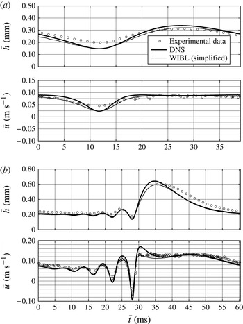
Comparison of experimental (Dietze Reference Dietze2010) and numerical results for the cases of table 1: (a) case 1,
 $\mathit{Re}_{\overline{q}}=6.8$
; (b) case 2,
 $\mathit{Re}_{\overline{q}}=15$
. The streamwise velocity is given at 0.1 mm from the plate.

In order to examine the experimental conditions numerically, the a priori unknown wavelength (i.e. domain size of the DNS) and initial film thickness (i.e. thickness-based Reynolds number) have been iteratively adjusted such that the flow rate,
 $\mathit{Re}_{\overline{q}}$
, and the frequency between simulations and experiment match (table 1). For DNS and WIBL simulations, equivalent flow conditions have been applied, whereby the dimensionless wavenumber is
 $$\begin{eqnarray}k_{x}=\frac{2{\rm\pi}}{{\it\lambda}_{x}}{\it\kappa}\overline{h}_{N}.\end{eqnarray}$$
Quantitative comparisons for the dimensional film thickness
 $\bar{h}$
and the streamwise velocity
 $\bar{u}$
(at the crosswise position
 $\bar{y}=0.1~\text{mm}$
) are shown in figure 8. For
 $\mathit{Re}_{\overline{q}}=6.8$
, the film thickness of the WIBL model and the DNS are in very good agreement. However, the film thickness amplitude of the experimental results is slightly lower compared with the simulations. Similar agreement is found for the streamwise velocity. For
 $\mathit{Re}_{\overline{q}}=15$
, the film thickness profiles of the WIBL model and the DNS agree very well in the capillary region, for the residual layer and for the back of the wave. The wave front is found to be steeper and the wave peak height is increased by approximately 8 % in the DNS results. In comparison with the experimental data, the highest deviations are found in the region of the wave’s back, which has more concave shape in both simulations compared to the experiment. The streamwise velocity beneath the wave crest at
 $\bar{y}=500~{\rm\mu}\text{m}$
was found experimentally to be between
 $0.34$
and
 $0.36~\text{m}~\text{s}^{-1}$
(Dietze Reference Dietze2010, not shown) and is already larger than the wave speed of
 $\bar{c}_{DNS}=0.328~\text{m}~\text{s}^{-1}$
and
 $\bar{c}_{WIBL}=0.3395~\text{m}~\text{s}^{-1}$
obtained by the two numerical approaches. Although the wave celerity was not measured experimentally, the comparison suggests the existence of circulating waves for the experimental conditions examined.
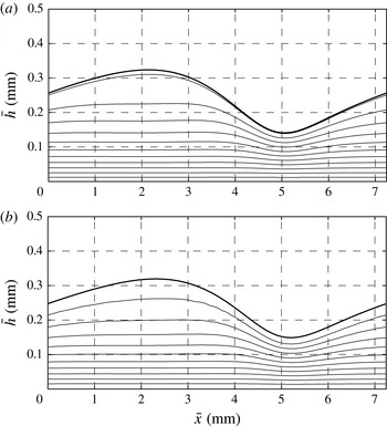
Wave topology (thick line) and flow field (streamlines) for case 1, for closed flow condition with
 ${\it\delta}_{\overline{h}_{N}}=4.28$
, i.e.
 $\mathit{Re}_{\overline{h}_{N}}=5.99$
,
 ${\it\zeta}=0$
and
 ${\it\eta}=0.057$
: (a) full second-order WIBL model,
 $\bar{{\it\psi}}=[2,4,6,\dots ,22]\times 10^{-6}~\text{m}^{2}~\text{s}^{-1}$
,
 $\bar{c}=0.1762~\text{m}~\text{s}^{-1}$
; (b) DNS,
 $\bar{{\it\psi}}=[2,4,6,\dots ,20]\times 10^{-6}~\text{m}^{2}~\text{s}^{-1}$
,
 $\bar{c}=0.1736~\text{m}~\text{s}^{-1}$
. The range of the dimensional stream function is as shown in brackets.

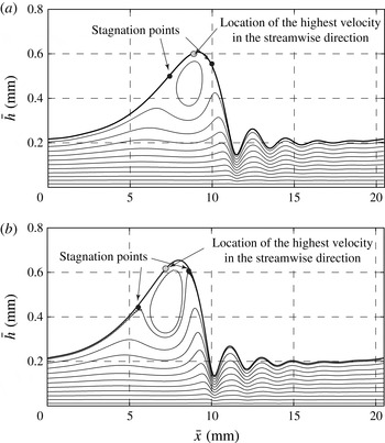
A comparison between the two methods (full second-order WIBL and DNS) for the wave topology and flow field is shown in figures 9 and 10 for cases 1 and 2, respectively. The stream function
 ${\it\psi}$
has been calculated from the velocity field (see appendix B), including corrections to the parabolic profile. The agreement between the two methods for case 1, characterized by the absence of circulating waves, is excellent. For case 2, for both methods the streamlines show circulating fluid in the main wave hump. Although the main flow behaviour is identical in both simulations, a difference is found in the position and the shape of the recirculation zone. In the results obtained by the WIBL model, the centre of the roll is located closer to the position of maximum film thickness. In contrast, the position of the vortex in the DNS is located behind the wave crest and is significantly stretched in the cross-stream direction. Additionally, the positions of the stagnation points are different. The shape found in the DNS agrees with the experimental observation of Alekseenko et al. (Reference Alekseenko, Antipin, Bobylev and Markovich2007) and the numerical results obtained by Wasden & Dukler (Reference Wasden and Dukler1989) and Islam (Reference Islam2009). The DNS results also reveal the global maximum of the streamwise velocity (marked in the plot) to be located not at the point of highest film thickness but at the wave’s back, significantly below the wave crest.
Same as figure 9 for case 2, with
 ${\it\delta}_{\overline{h}_{N}}=8.747$
, i.e.
 $\mathit{Re}_{\overline{h}_{N}}=10.76$
,
 ${\it\zeta}=0$
and
 ${\it\eta}=0.073$
: (a) full second-order WIBL model,
 $\bar{{\it\psi}}=[0,5,10,\dots ,55,58,60]\times 10^{-6}~\text{m}^{2}~\text{s}^{-1}$
,
 $\bar{c}=0.3375~\text{m}~\text{s}^{-1}$
; (b) DNS,
 $\bar{{\it\psi}}=[0,5,10,\dots ,50,54,55]\times 10^{-6}~\text{m}^{2}~\text{s}^{-1}$
,
 $\bar{c}=0.328~\text{m}~\text{s}^{-1}$
.

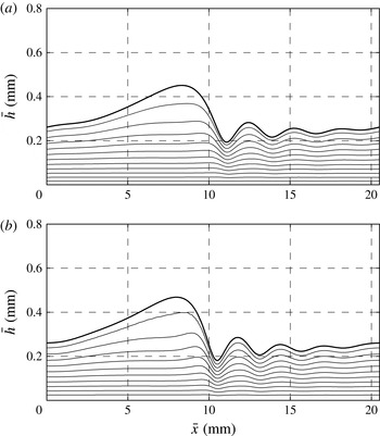
Same as figure 10 for an inclined plate, i.e.
 ${\it\zeta}=1$
: (a) full second-order WIBL model,
 $\bar{{\it\psi}}=[0,5,\dots ,55]\times 10^{-6}~\text{m}^{2}~\text{s}^{-1}$
,
 $\bar{c}=0.312~\text{m}~\text{s}^{-1}$
; (b) DNS,
 $\bar{{\it\psi}}=[0,5,\dots ,55]\times 10^{-6}~\text{m}^{2}~\text{s}^{-1}$
,
 $\bar{c}=0.310~\text{m}~\text{s}^{-1}$
.

Onset of circulating waves according to (3.5): wave topology and film thickness profile calculated by the full second-order WIBL model for closed flow condition corresponding to case 2 for an inclined plate, i.e.
 ${\it\zeta}=0.3958$
;
 $\bar{{\it\psi}}=[0,5,10,\dots ,55]\times 10^{-6}~\text{m}^{2}~\text{s}^{-1}$
;
 $\bar{c}=0.325~\text{m}~\text{s}^{-1}$
.

3.2.2. Dissection of wave features for inclined plates
The suppression of circulating waves by a volume force acting in the direction normal to the wall (i.e. gravity) for the same Reynolds number as examined in case 2 is shown in figure 11. Again, the direct numerical and the integrated boundary layer approaches reveal very similar results. Figure 12 depicts the streamlines for the onset of circulating waves (
 ${\it\zeta}=0.3958$
) at which the condition of (3.5), based on the parabolic velocity profile, is fulfilled. The streamline plot including the first-order velocity corrections (see (B 1) in appendix B) shows the existence of two stagnation points located close to the wave crest. The streamwise velocity between the two points exceeds the wave speed
 $c$
, such that the onset of circulating waves occurs slightly earlier. However, the short distance between the two stagnation points validates the simplification of the first-order velocity profile used to derive (2.11), hence (3.5).
The ratio between maximum and minimum film thickness (
 $\bar{h}_{max}=537.2~{\rm\mu}\text{m}$
and
 $\bar{h}_{min}=163.1~{\rm\mu}\text{m}$
) is 3.29. Approximating the residual layer film thickness by the average film thickness between the first capillary’s minimum and maximum yields
 $\bar{h}_{s}=219.0~{\rm\mu}\text{m}$
and thus a ratio of
 $\bar{h}_{max}/\bar{h}_{s}=2.45$
, which is close to the threshold found by Maron et al. (Reference Maron, Brauner and Hewitt1989) (
 $\bar{h}_{b}/\bar{h}_{s}=[2.5{-}3]$
).
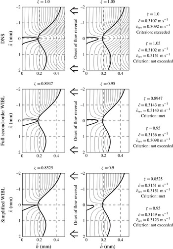
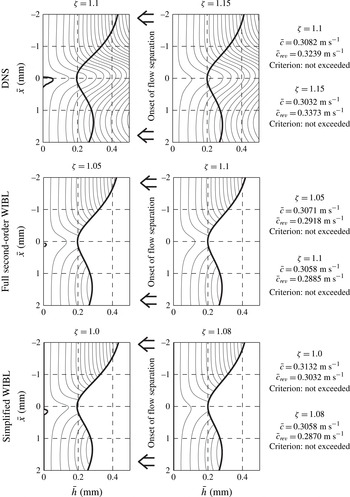
The transition from waves with flow reversal to waves without this feature is shown in figure 13, and the transition from waves with flow separation to waves without both characteristics is shown in figure 14. All simulation results are presented for case 2 using DNS and the WIBL model. As both phenomena are present in the case of a vertical plate (
 ${\it\zeta}=0$
), the inclination number has been increased stepwise up to the point where neither flow reversal nor flow separation exists. The left panels in figure 13 show the case where the criterion for the onset of flow reversal is met (WIBL) or slightly exceeded (DNS). Note that the inclination number for the transition is different, namely
 ${\it\zeta}_{DNS}\approx 1$
and
 ${\it\zeta}_{sWIBL}=0.85$
. In terms of the inclination angle
 ${\it\beta}$
, this translates to
 ${\it\beta}_{DNS}\approx 15.2$
and
 ${\it\beta}_{sWIBL}=17.7^{\circ }$
. The DNS and the full second-order model show a similar form of the separation vortex, with a steep gradient towards the main wave hump and a smaller gradient towards the first capillary maximum. Using the simplified model, the velocity over the entire cross-section is zero, for which both the flow rate and the first derivative of the flow rate must be zero (according to (B 1)). Besides the streamline plots, the wave celerity and the critical wave celerity for the onset of flow reversal are given for all 12 cases based on criterion (3.6) for DNS and based on the equivalent criterion (2.14) for the WIBL models. Criterion (2.14) has been used because
 $q_{0}$
is known from the WIBL simulations, contrary to the average flow rate
 $\langle q\rangle _{{\it\lambda}}$
. Note that the two criteria show different behaviour for larger values of
 ${\it\zeta}$
, such that the wave celerity is below the criterion in the DNS results for the absence of flow reversal, while for the WIBL results the wave celerity exceeds the criterion.
Onset of flow reversal: flow field (streamlines in a fixed frame of reference) in the region of the capillary minimum calculated by DNS and WIBL for closed flow condition with
 ${\it\delta}=8.747$
, i.e.
 $\mathit{Re}_{\overline{h}_{N}}=10.76$
:
 $\bar{{\it\psi}}=[0,-1.25,-5,-10,-15,\dots ]\times 10^{-6}~\text{m}^{2}~\text{s}^{-1}$
. Thick lines show the interface and the flow separation streamline with
 $\bar{{\it\psi}}=0$
.

Onset of flow separation: legend as in figure 13.

An increasing inclination number leads to a reduction in size of the separation vortex up to the point where it disappears. This transition process is found to be well captured by the WIBL model as suggested by the comparison of the streamline plots to the DNS results. However, the difference of the inclination number remains, such that the onset of flow separation occurs also for lower values of
 ${\it\zeta}$
in the WIBL model compared to the DNS.
3.2.3. Fixed frequency
The results of the DNS shown in the previous section were computed using periodic boundary conditions in streamwise direction. For consistency, the closed flow condition has been used in the WIBL model. However, experiments and applications are often characterized by a fixed flow rate at the inlet (
 $\mathit{Re}_{\overline{q}}$
or
 ${\it\delta}_{\overline{q}}$
) and, if excited externally, by an excitation frequency and not by a constant wavelength. Thus, we apply here the open flow boundary condition for the WIBL simulations. Consequently, the dimensionless flow rate takes a constant value of
 $\langle q\rangle _{{\it\lambda}}=1/3$
, for which the critical wave celerities for the onset of circulating waves and flow reversal given by (2.12) and (2.15) simplify to
 $$\begin{eqnarray}c_{circ}=\frac{1}{3\langle h\rangle _{{\it\lambda}}-h_{max}}\end{eqnarray}$$
and
 $$\begin{eqnarray}c_{rev}=\frac{1}{3(\langle h\rangle _{{\it\lambda}}-h_{min})},\end{eqnarray}$$
respectively.
In addition to the dimensionless parameters introduced earlier, we introduce the dimensionless frequency according to
 $$\begin{eqnarray}f=\overline{f}{\it\kappa}\frac{t_{{\it\nu}}l_{{\it\nu}}}{\overline{h}_{N}},\end{eqnarray}$$
where
 $\overline{f}$
denotes the dimensional frequency (in Hz), and
 $l_{{\it\nu}}=({\it\nu}^{2}/g\sin {\it\theta})^{1/3}$
and
 $t_{{\it\nu}}=({\it\nu}/(g\sin {\it\theta})^{2})^{1/3}$
denote the viscous length and time scale, respectively.
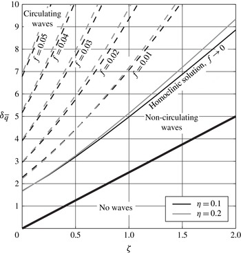
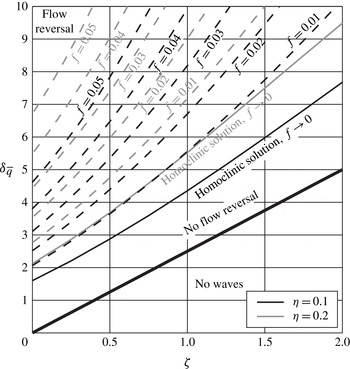
Figure 15 shows the phase diagram for the onset of circulating waves as a function of reduced inclination number
 ${\it\zeta}$
and dimensionless excitation frequency
 $f$
as well as for two different viscous dissipation numbers
 ${\it\eta}$
. The full second-order model is used for all calculations. The transition from no waves to non-circulating waves is plotted for homoclinic solutions, revealing the absolute stability of the film flow for low reduced Reynolds numbers and finite values of
 ${\it\zeta}$
. Additionally for comparison, the transition for the homoclinic solution is shown by the black line. The dashed lines illustrate the onset of circulating waves for higher frequencies, and thus for waves of shorter wavelength. Obviously, the Reynolds number at which the onset of circulating waves occurs increases with excitation frequency. A small increase in the threshold value with the viscous dissipation number is found, similar to the influence observed for the homoclinic solution.
Phase diagram for the onset of circulating waves as a function of reduced inclination number
 ${\it\zeta}$
and dimensionless excitation frequency
 $f$
. Data are obtained by using the full second-order model.

Based on the simulation results, a correlation equation for the critical reduced Reynolds number
 ${\it\delta}_{circ}$
can be deduced including the effect of finite frequencies. Expanding the correlation (3.3) established for the homoclinic orbit by introducing two frequency dependences (modifying the constant for
 ${\it\zeta}=0$
and the slope) yields
 $$\begin{eqnarray}{\it\delta}_{circ}=-(2+24\,f)+(2+{\it\zeta})^{1.76+23f},\end{eqnarray}$$
which fits the numerical data with
 $R^{2}=0.995$
for
 ${\it\eta}=0.1$
.
The same picture as for circulating waves can be drawn for flow reversal as shown in figure 16. A similar dependence of the onset on the excitation frequency
 $f$
is obtained, shifted towards higher values of the inclination number. Nevertheless, the significant influence of the viscous dissipation number, already observed for the homoclinic solution, is also found for finite limit cycles. Owing to the multifactorial dependence of the onset of flow reversal, a simple correlation function cannot be given.
Phase diagram for the onset of flow reversal as a function of reduced inclination number
 ${\it\zeta}$
and dimensionless excitation frequency
 $f$
. Data are obtained by using the full second-order model.

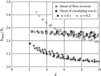
Figure 17 shows that the ratio between the maximum film thickness and the substrate thickness at the onset of circulating waves remains rather constant irrespective of the inclination, frequency and viscous dissipation number. Thus, this ratio can be a sufficiently suitable criterion for the onset of circulating waves. For the onset of flow reversal, the ratio between maximum film thickness and substrate film thickness indicated by the grey crosses is found to be dependent on Reynolds number and viscous dissipation number. The ratio decreases with both parameters, but does not depend on frequency.
Critical ratio between the maximum film thickness and the substrate film thickness at the onsets of circulating waves and flow reversal. The markers include results for different frequencies and inclination numbers. Data are obtained by using the full second-order model.

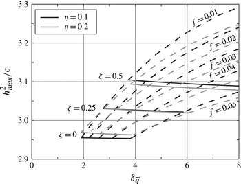
A comparison with the critical value for the onset of circulating waves proposed by Roberts & Chang (Reference Roberts and Chang2000) is shown in figure 18. According to their value for the critical wave speed, we have plotted the ratio between the square of the dimensionless maximum film thickness and the wave velocity. Following Roberts & Chang, this ratio should take a constant value of 2 whatever the frequency. Our results also reveal a nearly constant threshold for a vertical falling film (
 ${\it\zeta}=0$
), but with higher value of 2.95. The difference in the results arises from the assumption made by Roberts & Chang that the average velocity underneath the wave’s crest
 $q(x)/h(x)$
is equal to the averaged value of
 $1/3$
. Additionally, we would like to recall that the critical wave speed is
 $c_{circ}=1/(3\langle h\rangle _{{\it\lambda}}-h_{max})$
according to the WIBL model (3.5) and
 $c=h_{max}^{2}/2$
according to the assumption in Roberts & Chang. If inclination is also considered (
 ${\it\zeta}>0$
), the value of the ratio increases, but still remains rather constant on varying the frequency.
Validation of the criterion for the onset of circulating waves proposed by Roberts & Chang (Reference Roberts and Chang2000), i.e.
 $h_{max}^{2}/c=2$
. Data are obtained by using the full second-order model.

4. Conclusion
In this study, the onset of circulating waves and the onset of flow reversal has been investigated as a function of the Reynolds number and the inclination number
 ${\it\zeta}$
. For this, the simplified and full second-order WIBL models have been applied after validating the method with experimental data and DNS. An analytical criterion for the onset of circulating waves has been determined from the WIBL model based on the wave celerity, the average film thickness and the maximum film thickness (2.12). For the onset of flow reversal, a similar criterion based on the minimum film thickness is given (2.15). In addition, flow separation and the transition from drag–gravity to drag–inertia regimes have been considered.
It has been found by the numerical simulations that the onset of circulating waves and the transition from the drag–gravity to the drag–inertia regime are not significantly influenced by the viscous dissipation number, and that the critical reduced Reynolds number increases significantly for inclined film flows. In contrast, the onset of flow reversal is significantly influenced by the viscous dissipation number. For low values of the viscous dissipation number, the onset of circulating waves occurs for higher Reynolds numbers than the onset of flow reversal in the first capillary minimum. For high values of the viscous dissipation number, the transition changes. The results of this study also reveal that the threshold for the onset of circulating waves based on the ratio between maximum and substrate film thicknesses is appropriate.
Simulation results in the limit cycle, i.e. on a finite domain length, reveal a strong increase of the threshold Reynolds number with the excitation frequency for both flow reversal and recirculation. Nevertheless, the ratio between the maximum film thickness and the substrate film thickness is found to be rather constant for the onset of flow recirculation irrespective of the inclination, frequency and viscous dissipation number. For the onset of flow reversal, this ratio is found to decrease with Reynolds number and to be dependent on the dissipation number, but not on the excitation frequency. These findings support the practical use of the results obtained by the homoclinic solution. Finally, a correlation equation (3.11) is given for the critical reduced Reynolds number at the onset of circulating waves as a function of the reduced inclination number and the dimensionless frequency. We believe that this correlation, together with the definitions (2.3) and (2.4), can be of practical interest for future experimental identification of the different phase regions, as each phase change is believed to have a significant influence on heat transfer behaviour.
Acknowledgements
We thank G. Dietze for his fruitful comments and questions with respect to the onset of flow separation and C. Ruyer-Quil for his advice regarding the Froude number. We acknowledge the financial support of EU-FP7 ITN Multiflow as well as the BELSPO agency under the grant IAP-7/38 MicroMAST. B.S. also thanks the FRS-FNRS for financial support.
Appendix A
The four evolution equations for the full second-order model read
 $$\begin{eqnarray}\partial _{t}h=\partial _{x}q,\end{eqnarray}$$
 $$\begin{eqnarray}\displaystyle {\it\delta}\partial _{t}q & = & \displaystyle \frac{27}{28}h-\frac{81}{28}\frac{q}{h^{2}}-33\frac{s_{1}}{h^{2}}-\frac{3069}{28}\frac{s_{2}}{h^{2}}-\frac{27}{28}{\it\zeta}h\partial _{x}h+\frac{27}{28}h\partial _{xxx}h\nonumber\\ \displaystyle & & \displaystyle +\,{\it\delta}\left(-\frac{12}{5}\frac{qs_{1}\partial _{x}h}{h^{2}}-\frac{126}{65}\frac{qs_{2}\partial _{x}h}{h^{2}}+\frac{12}{5}\frac{s_{1}\partial _{x}q}{h}+\frac{171}{65}\frac{s_{2}\partial _{x}q}{h}\right.\nonumber\\ \displaystyle & & \displaystyle \left.+\,\frac{12}{5}\frac{q\partial _{x}s_{1}}{h}+\frac{1017}{455}\frac{q\partial _{x}s_{2}}{h}+\frac{6}{5}\frac{q^{2}\partial _{x}q}{h^{2}}-\frac{12}{5}\frac{q\partial _{x}q}{h}\right)\nonumber\\ \displaystyle & & \displaystyle +\,{\it\eta}\left(\frac{5025}{896}\frac{q(\partial _{x}h)^{2}}{h^{2}}-\frac{5055}{896}\frac{\partial _{x}q\partial _{x}h}{h}-\frac{10851}{1792}\frac{q\partial _{xx}h}{h}+\frac{2027}{448}\partial _{xx}q\right),\end{eqnarray}$$
 $$\begin{eqnarray}\displaystyle {\it\delta}\partial _{t}s_{1} & = & \displaystyle \frac{1}{10}h-\frac{3}{10}\frac{q}{h^{2}}-\frac{126}{5}\frac{s_{1}}{h^{2}}-\frac{126}{5}\frac{s_{2}}{h^{2}}-\frac{1}{10}{\it\zeta}h\partial _{x}h+\frac{1}{10}h\partial _{xxx}h\nonumber\\ \displaystyle & & \displaystyle +\,{\it\delta}\left(-\frac{3}{35}\frac{q^{2}\partial _{x}h}{h^{2}}+\frac{1}{35}\frac{q\partial _{x}q}{h}+\frac{108}{55}\frac{qs_{1}\partial _{x}}{h^{2}}-\frac{5022}{5005}\frac{qs_{2}\partial _{x}h}{h^{2}}\right.\nonumber\\ \displaystyle & & \displaystyle \left.-\,\frac{103}{55}\frac{s_{1}\partial _{x}q}{h}+\frac{9657}{5005}\frac{s_{2}\partial _{x}q}{h}-\frac{39}{55}\frac{q\partial _{x}s_{1}}{h}+\frac{10557}{10010}\frac{q\partial _{x}s_{2}}{h}\right)\nonumber\\ \displaystyle & & \displaystyle +\,{\it\eta}\left(\frac{93}{40}\frac{q(\partial _{x}h)^{2}}{h^{2}}-\frac{69}{40}\frac{\partial _{x}q\partial _{x}h}{h}+\frac{21}{80}\frac{q\partial _{xx}h}{h}-\frac{9}{40}\partial _{xx}q\right),\end{eqnarray}$$
 $$\begin{eqnarray}\displaystyle {\it\delta}\partial _{t}s_{2} & = & \displaystyle \frac{13}{420}h-\frac{13}{140}\frac{q}{h^{2}}-\frac{39}{5}\frac{s_{1}}{h^{2}}-\frac{11817}{140}\frac{s_{2}}{h^{2}}-\frac{13}{420}{\it\zeta}h\partial _{x}h+\frac{13}{420}h\partial _{xxx}h\nonumber\\ \displaystyle & & \displaystyle +\,{\it\delta}\left(-\frac{4}{11}\frac{qs_{1}\partial _{x}h}{h^{2}}+\frac{18}{11}\frac{qs_{2}\partial _{x}h}{h}-\frac{2}{33}\frac{s_{1}\partial _{x}q}{h}-\frac{19}{11}\frac{s_{2}\partial _{x}q}{h}\right.\nonumber\\ \displaystyle & & \displaystyle \left.+\,\frac{6}{55}\frac{q\partial _{x}s_{1}}{h}-\frac{288}{385}\frac{q\partial _{x}s_{2}}{h}\right)\nonumber\\ \displaystyle & & \displaystyle +\,{\it\eta}\left(-\frac{3211}{4480}\frac{q(\partial _{x}h)^{2}}{h^{2}}+\frac{2613}{4480}\frac{\partial _{x}q\partial _{x}h}{h}-\frac{2847}{8960}\frac{q\partial _{xx}h}{h}+\frac{559}{2240}\partial _{xx}q\right).\end{eqnarray}$$
Appendix B
The velocity field obtained in deriving the second-order WIBL model is calculated by evaluating the streamwise and cross-stream velocities (for details, see e.g. Kalliadasis et al. Reference Kalliadasis, Ruyer-Quil, Scheid and Velarde2013). The streamwise velocity, including the first-order corrections to the parabolic velocity profile, is given by
 $$\begin{eqnarray}\displaystyle u(x,y) & = & \displaystyle \frac{{\it\delta}}{140h^{7}}(hy-{\textstyle \frac{1}{2}}y^{2})\big\{21y^{4}q^{2}h_{x}-28ch^{6}q_{x}+2h^{5}(35cy+36q)q_{x}\nonumber\\ \displaystyle & & \displaystyle -\,7y^{3}hq(12qh_{x}+yq_{x})+14y^{2}h^{2}q(3qh_{x}+2yq_{x})+28yh^{3}q(3qh_{x}+2yq_{x})\nonumber\\ \displaystyle & & \displaystyle -\,h^{4}[48q^{2}h_{x}+35cy^{2}q_{x}+84q(-5/{\it\delta}+2yq_{x})]\big\},\end{eqnarray}$$
and the cross-stream velocity is straightforwardly calculated based on
 $$\begin{eqnarray}v(x,y)=\int _{0}^{y}\frac{\partial (u(x,Y))}{\partial x}\,\text{d}Y.\end{eqnarray}$$
For the evaluation of the shear stress, the derivative of (B 1) is evaluated at the wall
 $(y=0)$
, leading to
 $$\begin{eqnarray}{\it\tau}_{W}(x)=\frac{1}{35h^{2}}[-12{\it\delta}q^{2}h_{x}-7c{\it\delta}h^{2}q_{x}+3q(35+6{\it\delta}hq_{x})].\end{eqnarray}$$