3.1 Steady axisymmetric flow with magnetic field

When $20<Re<210$ in the absence of a magnetic field, the flow is steady, axisymmetric and topologically similar. Only the separation length and the separation angle of the separation bubble vary with different Reynolds numbers. Here, only the case at $Re=150$ is considered. Since the flow is axisymmetric, any magnetic field direction in the transverse plane has the same effect on the wake structure. So only results of the $y$ -directional transverse magnetic field are given below. Skin friction lines on the sphere surface with different interaction parameters are presented in figure 3. It is noted that convergence of skin friction lines is a criterion of three-dimensional flow separation (Lighthill Reference Lighthill and Rosenhead1963). Skin friction lines can clearly show flow traces in the rear of the sphere, which help us analyse the wake structure. As shown in figure 3, the shape of the flow separation line is narrowed in the P-symmetry plane at $N=0.3$ , which changes from a circular shape at $N=0$ to an approximately elliptical shape. At this stage, the flow separation line is closed; skin friction lines in the inner part of the closed separation line come from recirculation flows. This means that a recirculation region still exists. However, with an increasing magnetic field at $N=1$ , the closed separation line disappears, which means the recirculation region is gone. Shatrov, Mutschke & Gerbeth (Reference Shatrov, Mutschke and Gerbeth1997) also found that a transverse magnetic field could lead to a complete suppression of recirculation on a two-dimensional flow past a cylinder. Now the upstream flow converges into two symmetric points at the rear of the sphere surface. Further increasing the magnetic field at $N=4$ , the convergence points disappear and a straight separation line in the N-symmetry plane is clearly visible. Obviously, the non-axisymmetry of the wake structure is expected when affected by a transverse magnetic field. Now the wake structure is double plane symmetric and its symmetry planes are P- and N-symmetry planes.

Figure 3.

Skin friction lines on the sphere surface at $Re=150$ with different interaction parameters: (a)  $N=0$ , (b)  $N=0.3$ , (c)  $N=1$ and (d)  $N=4$ . The flow direction is from inside to outside. The magnetic field direction is from bottom to top.

Assuming that the sphere is absent in the flow, currents coming from electromotive forces are dominant in the core flow, which are generated by the fluid motion and represented by $\boldsymbol{u}\times \boldsymbol{B}$ in the Ohm’s law (2.3). When considering a sphere, the flow field mainly can be divided into two parts. One part is far away from the sphere, where electromotive forces $\boldsymbol{u}\times \boldsymbol{B}$ are dominant. Currents in this part flow from right to left, as shown at the B position of figure 4(a). The other part is near the sphere, where the velocity $\boldsymbol{u}$ must be weaker. Positive charges are concentrated in the left side of the sphere (red colour) while negative charges are concentrated in the right side of the sphere (blue colour). The charge conservation law requires that current lines need to be closed. Since velocity is weaker here, electric potential gradients are dominant, where currents flow from left to right, as shown at the C position of figure 4(a). Furthermore, the sphere is electrically insulating. Currents will not go into the sphere, but flow over the surface instead, as shown from A to C positions in the side view of figure 4(b).

Figure 4.

Current lines at $Re=150$ with $N=1$ . The results are plotted at time instant $T_{i}=7\unicode[STIX]{x0394}t$ after imposing a transverse magnetic field. Here $\unicode[STIX]{x0394}t$ is the time step in the simulation. The magnetic field direction is from bottom to top. (a) Front view. The flow direction is from inside to outside. Current lines are contoured with $x$ component of the Lorentz force, for which the positive direction is from left to right. The sphere is contoured with the electric potential, for which the red colour means positive value while the blue one represents negative value. (b) Side view. The flow direction is from left to right.

Figure 5.

Lorentz force at $Re=150$ with $N=1$ in a front view for figure 4(a). The flow direction is from inside to outside. (a) Schematic for the Lorentz force acting on the upstream flow with a small interaction parameter. The red dashed line represents the separation line. The black and red arrows represent the upstream flow projected on the transverse plane and the Lorentz force on the transverse plane, respectively. The blue curved arrow shows the moving trend of the upstream flow affected by the Lorentz force. (b) The $z$ -component of the Lorentz force contours in a section $0.35d$ away from the sphere centre.

After understanding the current distribution, it is easy to know the Lorentz force $\boldsymbol{J}\times \boldsymbol{B}$ exerted on the flow. Since currents flow over the sphere surface from A to C positions in figure 4(b), the $z$ -component of current $J_{z}$ exists and will interact with the magnetic field to generate the $x$ -component of the Lorentz force. Figure 4(a) shows the $x$ -component of the Lorentz force contours on the current lines. These forces pull the upstream flow away from the P-symmetry plane to two lateral sides of the sphere. Figure 5(a) shows a schematic for the $x$ -component of the Lorentz force acting on the upstream flow at a small interaction parameter. As a result, the upstream flow around the sphere diverges from the P-symmetry plane and converges to the N-symmetry plane. The blue curved arrows in figure 5(a) show this moving trend. The Lorentz force at position C of figure 4(a) is interesting – it will accelerate rather than damp the upstream flow. The $z$ -component of the Lorentz force contours are plotted in figure 5(b). The $z$ -component of the Lorentz force in zone D is larger than that in zone E since the currents are clustered in zone D, which corresponds to a faster flow near the surface in zone D. Hence this flow drives the flow separation line from a circular shape into an approximately elliptical shape, as shown in figure 4(a). Figure 6 shows such a recirculation of elliptical shape in detail. One quarter of the three-dimensional streamlines at $N=0.1$ behind the sphere are plotted in figure 6(a). The direction of the core flow connecting two spirals reflects the moving trend of the upstream flow around the sphere. Such a moving trend will squeeze flow in the N-symmetry plane and make the left vortex in figure 6(a) spiral outwards. At the same time, the right vortex spirals inwards as it serves as the source of the core flow. Figures 6(b) and 6(c) show such spirals in the P- and N-symmetry plane. These two spirals will become smaller and finally disappear with increasing magnetic field.

Figure 6.

Pressure contours and streamlines in the symmetry plane at $Re=150$ with $N=0.1$ . The magnetic field direction is along the $y$ -axis. (a) One quarter of the three-dimensional streamlines. (b) P-symmetry plane. (c) N-symmetry plane.

Figure 7.

Time evolution of skin friction lines on the sphere surface at $Re=150$ with $N=1$ . The results are plotted at different time instants after imposing a transverse magnetic field: (a)  $T_{i}=27\unicode[STIX]{x0394}t$ , (b)  $T_{i}=167\unicode[STIX]{x0394}t$ and (c)  $T_{i}=267\unicode[STIX]{x0394}t$ , where $\unicode[STIX]{x0394}t$ is the time step in the simulation. The flow direction is from inside to outside. The magnetic field direction is from bottom to top.

Continuing with figure 4(a), figure 7 shows the time evolution of skin friction lines on the sphere surface. The recirculation region first becomes smaller in figure 7(a) and then disappears in figure 7(b). Now the upstream flow directly flows over the sphere surface and converges at the N-symmetry plane. At this stage, the $x$ -component Lorentz force competes with the pressure gradient between the front and rear of the sphere, for which the Lorentz force pulls away the upstream flow from the P-symmetry plane and the pressure gradient pushes the upstream flow towards the P-symmetry plane. When the $x$ -component Lorentz force is dominant, upstream flows will go away from the P-symmetry plane and converge at two points, as shown in figure 7(c). Further increasing the magnetic field, pressure gradients become dominant and a straight separation line will remain at the N-symmetry plane. The final stable states in figures 3(c) and 3(d) correspond to these two situations.

3.2 Unsteady plane symmetric flow with magnetic field

3.2.1 Unsteady flow with weak magnetic field

It is known that the onset of unsteadiness for a flow past a sphere without a magnetic field occurs at $Re\approx 270$ and large-scale vortical structures are shed periodically at $Re=300$ . Regardless of the certain orientation of the symmetry plane, $x$ -directional and $y$ -directional transverse magnetic fields are imposed, respectively. For a weak magnetic field situation, the flow is still unsteady with vortex shedding. In order to quantify how the Lorentz force damps vortex shedding, a distance length $H$ defined in Pan et al. (Reference Pan, Zhang and Ni2018) is used here, which presents the tilt of recirculation behind the sphere, as shown in figure 8(a). In a period of vortex shedding, the tilt of recirculation varies with time. Time evolution of the distance length for different interaction parameters during one period is plotted in figure 8(b). The amplitude is much damped by the transverse magnetic field at $N=0.01$ . The $x$ -directional and $y$ -directional transverse fields have the same influences on the wake behind the sphere, which is also confirmed by the identical time history of drag and lift coefficients in figure 8(c).

Figure 8.

Time evolution at $Re=300$ with different interaction parameters. The magnetic field is along the $x$ - or $y$ -direction. (a) Schematic for the distance length $H$ between the stagnation point and the axis along the sphere centre. (b) Time evolution of distance length during one vortex shedding period $T$ . The time is scaled with $T$ . (c) Time history of drag and lift coefficients. The time is scaled with $d/U_{0}$ . These coefficients are both scaled with ${\textstyle \frac{1}{2}}\unicode[STIX]{x1D70C}U_{0}^{2}A$ , where $A$ is the transverse section area of the sphere.

After vortices are shed from the sphere, they are advected downstream. Figure 9 shows the power spectra of the streamwise velocity at point $(0,0,6d)$ behind the sphere for $N=0$ , and for $N=0.01$ in the $x$ - and $y$ -directions. It is clearly seen that the same shedding frequency $S_{t}=0.136$ is found at $N=0.01$ for $x$ -directional and $y$ -directional transverse magnetic fields, which means that both fields have the same influences on the downstream wake flow. Compared with the case with no magnetic field at $N=0$ , the shedding frequency is unchanged. Hence, the transverse magnetic field affects only the amplitude and not the frequency of vortex shedding. Numerical (Mutschke et al. Reference Mutschke, Gerbeth, Shatrov and Tomboulides2001) and experimental (Lahjomri et al. Reference Lahjomri, Capéran and Alemany1993) results found that flow past a cylinder with an increasing streamwise magnetic field led to a slightly reduced shedding frequency. Shatrov et al. (Reference Shatrov, Mutschke and Gerbeth1997) claimed that an increasing streamwise magnetic field caused a reduction of the mean separation angle of a two-dimensional cylinder flow, which should lead to a slightly smaller shedding frequency. However, for the present sphere case, the separation line during the vortex shedding process is nearly unaffected by the influence of a weak transverse magnetic field at $N=0.01$ . The Lorentz force mainly affects the tilt of the recirculation and the separation angle remains unchanged. This may be the reason for the same shedding frequency. Such unchanged shedding frequency phenomenon is also found in the case of flow past a sphere with a streamwise magnetic field (Pan et al. Reference Pan, Zhang and Ni2018). Furthermore, a stronger damping of the superharmonics can be seen in figure 9. The same phenomenon is also reported for a streamwise magnetic field case in Pan et al. (Reference Pan, Zhang and Ni2018). For $x$ -directional or $y$ -directional transverse magnetic fields, the different initial angle $\unicode[STIX]{x1D703}$ impacts the time scale of the wake going to the final equilibrium state (see § 3.3), which causes the different amplitude of the frequency of the superharmonics in figure 9.

Figure 9.

Power spectra of the streamwise velocity component at $x=0,~y=0,~z=6d$ behind the sphere at $Re=300$ with $N=0$ or $N=0.01$ (semi-log plots). The magnetic field is along the $x$ - or $y$ -direction.

Three-dimensional large-scale vortical structures in the near-wake region of the sphere are shown by streamwise vorticity in figure 10. In figure 8(b), the degree of tilt is greatly damped by the magnetic field, so the smaller tilt converts less azimuthal vorticity into streamwise vorticity. Hence, a smaller streamwise vorticity is shown in figure 10(b).

Figure 10.

Streamwise vortical structures at $Re=300$ with different interaction parameters: (a)  $N=0$ and (b)  $N=0.01$ . Isosurfaces of streamwise vorticity with $\unicode[STIX]{x1D714}_{z}\pm 0.4$ . The red streamwise vorticity is positive while the blue one is negative.

3.2.2 Steady flow under an increasing magnetic field

Shatrov et al. (Reference Shatrov, Mutschke and Gerbeth1997) reported that the unsteady vortex shedding of a two-dimensional flow past a cylinder would be suppressed and transitioned to a steady flow affected by a transverse magnetic field. Then a stronger transverse magnetic field could lead to a complete suppression of recirculation. Similar results can be found for the present sphere case. Under an increasing magnetic field, the oscillation of the distance length $H$ in figure 8(b) will be completely suppressed. The periodic state transitions to a steady state at $N=0.015$ . 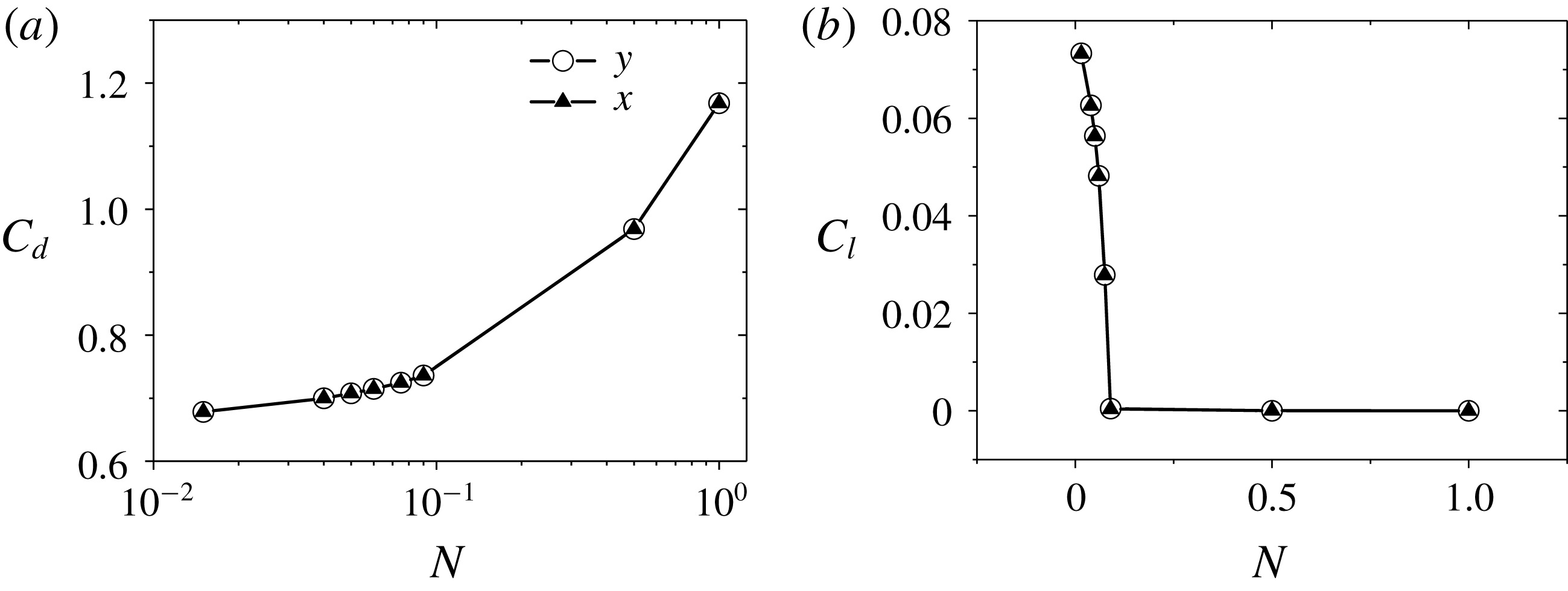But the distance length itself is still larger than zero, which means the tilt of recirculation behind the sphere still exists. The flow is now steady, plane symmetric and a constant lift force is in the symmetry plane. In § 3.2.1, $x$ -directional and $y$ -directional transverse magnetic fields have the same influences on unsteady wake structures. This conclusion is also suitable for steady wake structure situations, since figure 11 shows identical drag and lift coefficients. Remember that the flow past a sphere is first simulated for a long enough time and then a transverse magnetic field is imposed. In order to check whether the different initial time instants for imposing a transverse magnetic field have an influence on the final steady state, four time instants of a period as the starting points in figure 8(b) are tested at $N=0.04$ . All results are identical, which indicates that the starting time of imposing a magnetic field does not affect the final results, and the present steady results are consistent. Furthermore, the lift coefficient in figure 11(b) decreases with an increasing magnetic field and then remains zero. It should be noted that the non-zero lift zone corresponds to a plane symmetric state with tilt of recirculation behind the sphere while the flow in the zero lift zone corresponds to a double plane symmetric state. Here, a transition occurs at $C_{l}=0$ .

Figure 11.

Drag and lift coefficients of steady flows at $Re=300$ versus the interaction parameter with a magnetic field along $x$ - or $y$ -direction: (a)  $C_{d}$ (semi-log plots) and (b)  $C_{l}$ .

Figure 12.

Pressure contours and streamlines in the symmetry plane at $Re=300$ steady flow with different interaction parameters. The magnetic field direction is along the $y$ -direction. (a) P-symmetry plane at $N=0.015$ . (b) P-symmetry plane at $N=0.04$ . (c) P-symmetry plane at $N=0.09$ . (d) N-symmetry plane at $N=0.015$ . (e) N-symmetry plane at $N=0.04$ . (f) N-symmetry plane at $N=0.09$ .

Figure 12 shows detailed changes of topological structures, indicating that the wake structure is symmetric in the P-symmetry plane and the small left spiral in the N-symmetry plane will grow until it becomes the same as the right spiral. Now the lift force is zero and a transition from a steady plane symmetric flow to a steady double plane symmetric one occurs. With a further increasing magnetic field, the topological structure behind the sphere at $Re=300$ will go through the same patterns that happened at $Re=150$ in figure 3. With Reynolds numbers up to 300, a steady axisymmetric flow and an unsteady flow affected by a transverse magnetic field have been investigated. It is noted that, for a steady plane symmetric flow at $210<Re<270$ , the topological structure of the wake behind the sphere affected by a transverse magnetic field will go through the same changes as the steady flow at $Re=300$ shown in figure 12. They both experience the small left spiral growing, a transition from plane symmetry to double plane symmetry. Hence, the results are not repeatedly presented here.

The wake structure behind the sphere will change from an unsteady plane symmetric pattern to a steady plane symmetric one when affected by a transverse magnetic field. At this stage, the recirculation at the rear of the sphere still exists. Its wake structure has a similar topological structure with the case at $210<Re<270$ in the absence of a magnetic field. An effective viscosity concept in a previous investigation (Pan et al. Reference Pan, Zhang and Ni2018) can be used to understand this phenomenon with a magnetic damping effect. This theory claims that the Lorentz force action on the flow can be seen as an effective viscosity and that increasing the magnetic field is equivalent to adding effective viscosity into a corresponding hydrodynamic flow case, which is equivalent to decreasing the effective Reynolds number. Consequently, the change of wake structure affected by an increasing magnetic field will experience a similar change of wake structure in a hydrodynamic flow case with decreasing Reynolds number. Hence, a so-called ‘reversion phenomenon’ (Pan et al. Reference Pan, Zhang and Ni2018) is also found, which indicates that the topological structure behind the sphere at a higher Reynolds number with a certain interaction parameter corresponds to a lower-Reynolds-number case with a lower interaction parameter. Finally, all wake structures will be damped to be a double plane symmetric state with a strong transverse magnetic field.

Figure 13.

Detailed wake flow at $Re=300$ with $N=16$ . (a) Three-dimensional streamlines at the rear of the sphere. The blue arrow is a jet flow, which is caused by convergence of upstream flow. (b) Contour of the streamwise velocity norm $U_{n}$ at the slice $z=1d$ behind the sphere. The velocity $U_{n}$ is scaled with the inlet velocity. Traces of cross-flow velocity are projected on the slice. (c) Streamwise vorticity contour at the slice $z=1d$ behind the sphere. The profile of the sphere is indicated by a dashed circle.

The double plane symmetric wake is further discussed below. Figure 13 shows a detailed wake flow at $Re=300$ with $N=16$ . With the reversion phenomenon, the topological structure in figure 13(a) is double plane symmetric, which corresponds to the same topological structure at $Re=150$ with $N=4$ in figure 3(d). Upstream flows converge at two sides of the straight separation line by the action of the Lorentz force. Under the mass conservation constraint, the flow velocity at these two zones is faster than the surrounding flow, as shown in figure 13(a,b), so there will be a jet flow, which heads downstream and meets with the low-speed outer upstream flow. Then the upstream flow is pushed away and has a swirl velocity to move downstream. Such interaction converts to a streamwise vorticity. Figure 13(c) plots the streamwise vorticity contours at the slice $z=1d$ behind the sphere, which confirms again that the wake structure is double plane symmetric.

3.3 Preferred orientation of the vortex symmetry plane

In § 3.2, it was reported that the wake structure behind the sphere showed the same quantitative changes affected by transverse magnetic fields with identical intensity and different angle $\unicode[STIX]{x1D703}$ , such as the tilt of recirculation, vortex shedding frequency, drag coefficient and lift coefficient. Now we pay attention to the relationship between the orientation of the symmetry plane and the transverse magnetic field. The dash-dotted line in figure 14 represents the symmetry plane at $Re=300$ with $N=0$ . As can be seen, after being affected by the $x$ -directional or $y$ -directional transverse magnetic field at $N=0.01$ , the new symmetry plane denoted by the solid line at time instant $T=300$ will rotate and tend to be perpendicular to the magnetic field. Apart from the unsteady flow, we also examine the steady plane symmetric flow in § 3.2.2. Detailed topological structures of these flows are shown in figure 12. Such ring vortex shifting generates a lift force within the symmetry plane, so the lift force orientation can represent the orientation of the symmetry plane. The lift force in the transverse plane can be decomposed into $x$ - and $y$ -components. Detailed lift force coefficients affected by two transverse magnetic fields are plotted in figure 15(a). The direction from the coordinate origin to the data point of the lift force represents the orientation of the symmetry plane. It is clearly seen that, under the influence of a transverse magnetic field, this orientation is completely perpendicular to the magnetic field in the final equilibrium state.

Figure 14.

Cross-section of streamwise vortical structures at 1.5 diameters behind the sphere is plotted at $Re=300$ with $N=0.01$ at time instant $T=300$ (not final stable state): (a)  $x$ -directional magnetic field and (b)  $y$ -directional magnetic field. The dash-dotted line and solid line represent the orientation of the original and new symmetry planes, respectively. The black and red arrows mean the magnetic field direction and the lift force direction, respectively. The profile of the sphere is indicated by a dashed circle.

Figure 15.

The orientation of the wake structure tends to be perpendicular to a transverse magnetic field. The red arrow represents the magnetic field direction. (a) Lift force $Cl_{x}$ – $Cl_{y}$ plot at $Re=300$ with different interaction parameters under the influence of a transverse magnetic field. (b) Lift force $Cl_{x}$ – $Cl_{y}$ plot at $Re=250$ with different interaction parameters under the influence of a streamwise magnetic field (Pan et al. Reference Pan, Zhang and Ni2018). (c) Lift force $Cl_{x}$ – $Cl_{y}$ plot at $Re=300$ with different initial symmetry planes under the influence of a transverse magnetic field. The dashed arrow represents the initial orientation of the symmetry plane at $N=0$ .

Figure 16 plots a schematic of how the Lorentz force affects the orientation of the symmetry plane. The tilt of recirculation behind the sphere is simply represented by a small and large spiral. The orientation is along these two spirals. In fact, the physical mechanism here is similar to the case in § 3.1. The moving trend of upstream flow affected by the action of the Lorentz force in figure 16(a) will rotate the orientation, and the faster upstream flow in zone D in figure 16(b) will squeeze the orientation. These two effects finally make the orientation lie in the N-symmetry plane, which is perpendicular to the magnetic field. Further details of the tilt of recirculation behind the sphere are plotted in figure 12(e). Some streamlines from the large spiral directly flow downstream. However, this is not the case for the similar topological structure affected by a streamwise magnetic field in Pan et al. (Reference Pan, Zhang and Ni2018). Since the moving trend of upstream flow not only rotates the orientation of the symmetry plane, but also converges flow near the N-symmetry plane, this will squeeze flow in the large spiral and make some flows spiral outwards and head downstream. The orientation of the symmetry plane at $Re=250$ affected by a streamwise magnetic field in Pan et al. (Reference Pan, Zhang and Ni2018) is also examined. However, the original symmetry plane at $N=0$ is unchanged in figure 15(b), which is different from the present transverse magnetic field case.

Figure 16.

Lorentz force at $Re=300$ , $N=0.04$ in a front view. The flow direction is from inside to outside. (a) Schematic for the moving trend of the upstream flow, which will affect the orientation of the symmetry plane. (b) The $z$ -component of the Lorentz force contours in a section $0.35d$ away from the sphere centre.

For the orientation of the symmetry plane without a magnetic field, the orientation in principle is random but is actually determined by perturbations in experiments or numerical biases (Johnson & Patel Reference Johnson and Patel1999). It has been reported in Ghidersa & Dušek (Reference Ghidersa and Dušek2000) that the symmetry plane can be selected randomly by perturbation with a spectral/spectral-element discretization method. However, in the present finite-volume-type numerical method it is difficult to impose a perturbation for a certain direction in a flow around a fixed sphere. In order to obtain different initial angle $\unicode[STIX]{x1D703}$ , one easy way is to change the transverse magnetic field direction. As seen in figure 15(a), the orientation of the symmetry plane is located at $N=0$ . Three kinds of magnetic field directions are considered, which are along the $y$ -axis positive direction, the $x$ -axis positive direction and the $x$ -axis negative direction. These three magnetic fields have different initial angle $\unicode[STIX]{x1D703}$ with the symmetry plane. Since the flow configuration and the numerical model are axisymmetric, the whole system of these three magnetic fields can be rotated around the $z$ -axis to be parallel to the $y$ -direction, as shown in figure 15(c). Now three cases with different initial symmetry planes at $N=0$ are affected by a transverse magnetic field. The lift force $Cl_{x}$ – $Cl_{y}$ plot as in figure 15(a) is given in figure 15(c). Owing to the symmetry breaking that occurs when going from the solution with two symmetry planes at $N=0.09$ to the solution with only one symmetry plane with $N<0.09$ , two equivalent solutions with one symmetry plane exist. Hence, the transition occurs at a pitchfork bifurcation.

Ern et al. (Reference Ern, Risso, Fabre and Magnaudet2012) reported that the wake structure behind a free-moving particle was related to its trajectories. So it is possible that the transverse magnetic field can control the trajectory of a free-moving particle by changing the orientation of its wake structure. A case is given below to show this control feature.

The freely rising sphere case at $G=165$ , $m^{\ast }=0.5$ in the absence of a magnetic field is chosen. Here, $G=U_{0}d/\unicode[STIX]{x1D708}$ is the Galileo number, which replaces the Reynolds number in a moving-body problem; $U_{0}=\sqrt{|1-m^{\ast }|gd}$ is the gravitational velocity scale, where $g$ is the acceleration of gravity and $m^{\ast }$ measures the ratio of particle density to fluid density. A moving-frame method coupled with sphere motion equations (Pan, Zhang & Ni Reference Pan, Zhang and Ni2019) is used to simulate a freely rising sphere. Figure 17(a) shows an oblique trajectory of the sphere, which agrees with the numerical result (Jenny, Dušek & Bouchet Reference Jenny, Dušek and Bouchet2004) and the experimental result (Horowitz & Williamson Reference Horowitz and Williamson2010). Figure 17(b) shows a double-threaded wake consisting of streamwise counter-rotating vortices. It is clearly seen that the wake structure is plane symmetric. Furthermore, these two vortices will induce a flow with the right-hand rule and then a force will be exerted on the sphere under the law of interaction, which leads to a horizontal velocity to compensate this force, as shown in figure 17(c). It is noted that the horizontal velocity is along the symmetry plane. Hence, the horizontal velocity can represent the orientation of the wake structure.

Figure 17.

Freely rising sphere at $G=165$ , $m^{\ast }=0.5$ without a magnetic field. (a) Oblique trajectory. (b) Isosurfaces of streamwise vorticity with $\unicode[STIX]{x1D714}_{z}\pm 0.3$ . The red streamwise vorticity is positive while the blue one is negative. (c) Cross-section plot of streamwise vortical structures at one diameter behind the sphere. The profile of the sphere is indicated by a dashed circle.

The reason to choose such a freely rising sphere is that it has a similar wake structure to a flow past a fixed sphere in § 3.2.2. They are both plane symmetric with a double-threaded wake. After the freely rising sphere reaches its stable state, $x$ -directional and $y$ -directional transverse magnetic fields are imposed respectively to show its control feature to the trajectory of the freely rising sphere. The horizontal velocity of the freely rising sphere is used to represent the direction of motion of the sphere in the horizontal plane. As shown in figure 18, under the influence of a transverse magnetic field, the horizontal velocity tends to be perpendicular to the magnetic field. The reason is that the transverse magnetic field rotates the wake structure behind the freely rising sphere to be perpendicular to itself, as shown in figure 19. Assuming one is standing on the free sphere centre to observe the flow field, the physical mechanism of wake structure rotation is similar to the fixed-sphere case. The only difference is that there is no constraint on the degrees of freedom of a freely rising sphere. Hence, the rotation of the wake structure will rotate the freely rising sphere by viscosity force, which will facilitate the fluid–solid system moving into a new equilibrium state. As shown in figure 17(c), the smaller the streamwise vorticity, the weaker induced flow it has, leading to a smaller horizontal velocity. Figure 19 shows that the streamwise vorticity becomes smaller under the damping effect of an increasing magnetic field. Its variation trend is the same as the change of the horizontal velocity in figure 18.

Figure 18.

Magnetic field can control a freely rising sphere moving at $G=165$ , $m^{\ast }=0.5$ under the influence of a transverse magnetic field. (a) Transverse velocity $V_{x}$ – $V_{y}$ plot for $x$ - and $y$ -directional magnetic field. (b) Transverse velocity $V_{x}{-}V_{y}$ plot with two opposite small perturbations. The free-moving sphere is first stable at $N=0.025$ and then the magnetic field changes to $N=0.01$ and $N=0.015$ with a small $x$ -direction perturbation of horizontal velocity exerted on the sphere.

Figure 19.

Cross-section plots of streamwise vortical structures affected by a transverse magnetic field at one diameter behind the freely rising sphere at $G=165$ , $m^{\ast }=0.5$ : (a)  $N=0.01$ , (b)  $N=0.015$ , (c)  $N=0.02$ , (d)  $N=0.01$ , (e)  $N=0.015$ and (f)  $N=0.02$ . The arrow indicates the magnetic field direction. The profile of the sphere is indicated by a dashed circle.

As shown in figure 18(a), a horizontal velocity transition occurs at $N=0.025$ , where the motion of the free-moving sphere transitions from an oblique trajectory to a vertical one. A small velocity perturbation along the $x$ -axis positive direction or the $x$ -axis negative direction is exerted on the free sphere when it rises vertically and, at the same time, the transverse magnetic field decreases from $N=0.025$ to $N=0.015$ or $N=0.01$ . Figure 18(b) shows two equivalent solutions where one symmetry plane exists. The transition also occurs at a pitchfork bifurcation.

Some control features are discussed here. Figure 20(a) plots a time history of the angle $\unicode[STIX]{x1D703}$ with an initial angle $\unicode[STIX]{x1D703}_{0}=26^{\circ }$ . The most attractive feature is that the transverse magnetic field can control the horizontal motion of the free sphere to be perpendicular to itself. Here, a threshold angle $\unicode[STIX]{x1D703}_{t}=81^{\circ }$ is defined, which means the angle $\unicode[STIX]{x1D703}$ reaches 90 % perpendicular to a magnetic field and one can say that the control effect is obvious when $\unicode[STIX]{x1D703}>\unicode[STIX]{x1D703}_{t}$ . In order to give a systematic investigation of the influence of the initial angle $\unicode[STIX]{x1D703}_{0}$ and the magnetic field intensity $N$ on the temporal evolution of the angle $\unicode[STIX]{x1D703}$ , a total of 25 cases are simulated. Figure 20(b) shows the evolving time of the angle $\unicode[STIX]{x1D703}$ from the initial angle $\unicode[STIX]{x1D703}_{0}$ to the threshold angle $\unicode[STIX]{x1D703}_{t}$ . It is clearly seen that it takes less time for a strong magnetic field to reach the angle $\unicode[STIX]{x1D703}_{t}$ . Apart from the evolving time, a horizontal migration ratio is defined by $V_{h}/V_{z}$ , where $V_{h}$ and $V_{z}$ are the terminal horizontal and vertical velocities of the free sphere. The horizontal migration ratio decreases with increasing magnetic field and shows a linear dependence of $N^{2.5}$ in the range $0.01\leqslant N\leqslant 0.02$ in figure 20(c).

Figure 20.

Control features at $G=165$ , $m^{\ast }=0.5$ with different initial angles and interaction parameters. The time is scaled with $d/U_{0}$ , where $U_{0}$ is the gravitational velocity. (a) Time history of the angle $\unicode[STIX]{x1D703}$ . The dashed line represents a threshold angle $\unicode[STIX]{x1D703}_{t}=81^{\circ }$ , which means the transverse velocity is 90 % perpendicular to the magnetic field. (b) The evolving time for different initial angles reaching 90 % perpendicular to a magnetic field. Solid points represent results of different cases. (c) Horizontal migration ratio defined by $V_{h}/V_{z}$ , where $V_{h}$ and $V_{z}$ are terminal horizontal and vertical velocities.

Further consideration about the temporal evolution of the angle $\unicode[STIX]{x1D703}$ to reach the equilibrium state is given in figure 21. In § 3.2.2, an effective viscosity concept is used to explain the ‘reversion phenomenon’, which claims that a magnetic damping effect is equivalent to adding effective viscosity into the case and this case reverses to a lower-Reynolds-number case with a lower interaction parameter. The ‘reversion phenomenon’ inspires us to use the magnetic damping time $\unicode[STIX]{x1D70F}=(\unicode[STIX]{x1D70E}B^{2}/\unicode[STIX]{x1D70C})^{-1}$ to scale the evolving time in figure 20(b). The interaction parameter $N=\unicode[STIX]{x1D70E}B^{2}d/\unicode[STIX]{x1D70C}U_{0}$ can be reformed as $N=d/U_{0}\unicode[STIX]{x1D70F}$ , so that we have the relation $\unicode[STIX]{x1D70F}=d/U_{0}N$ . For the present investigations, $d/U_{0}$ is a fixed value; hence with the time scaling $\unicode[STIX]{x1D70F}$ , the three-dimensional plot in figure 20(b) is reduced to a two-dimensional plot in figure 21(a), where the magnetic damping effects shrink together. This can be more clearly seen by comparing figure 20(a) and figure 21(a). The shape of the angle $\unicode[STIX]{x1D703}$ evolving curve is like a hyperbolic tangent function $\unicode[STIX]{x1D703}=90\,\text{tanh}(\unicode[STIX]{x1D6FD}T)$ , where $\unicode[STIX]{x1D6FD}$ is a parameter. As can be seen in figure 21(a), the time history of the angle $\unicode[STIX]{x1D703}$ can collapse together by horizontal translation and the collapsed curve is characterized by a hyperbolic tangent function. So for a case with an initial angle $\unicode[STIX]{x1D703}_{0}$ , the temporal evolution of the angle $\unicode[STIX]{x1D703}$ can be easily fitted with a hyperbolic tangent function

(3.1) $$\begin{eqnarray}\displaystyle \unicode[STIX]{x1D703}^{\prime }=\text{tanh}(\unicode[STIX]{x1D6FD}T+\text{atanh}(\unicode[STIX]{x1D703}_{0}^{\prime })). & & \displaystyle\end{eqnarray}$$

Here, $\unicode[STIX]{x1D703}^{\prime }=\unicode[STIX]{x1D703}/90$ and $\unicode[STIX]{x1D703}_{0}^{\prime }=\unicode[STIX]{x1D703}_{0}/90$ . It is noted that here the evolution time is scaled with the magnetic damping time, $T=t/\unicode[STIX]{x1D70F}=tNU_{0}/d$ . With some mathematical operations, the inverse function of the above equation is given as

(3.2) $$\begin{eqnarray}\displaystyle T={\displaystyle \frac{1}{\unicode[STIX]{x1D6FD}}}\,\text{atanh}\left({\displaystyle \frac{\unicode[STIX]{x1D703}^{\prime }-\unicode[STIX]{x1D703}_{0}^{\prime }}{1-\unicode[STIX]{x1D703}^{\prime }\unicode[STIX]{x1D703}_{0}^{\prime }}}\right). & & \displaystyle\end{eqnarray}$$

The only unknown parameter $\unicode[STIX]{x1D6FD}$ can be easily obtained by linear fitting with the 25 simulation results, which gives $\unicode[STIX]{x1D6FD}=0.75$ . Figure 21(c) shows good agreement between the fitted curves plotted with (3.1) and the simulation results.

The control feature of the transverse magnetic field is attractive. The present work is the first time that the field–wake–trajectory control mechanism has been analysed for a particle freely moving in MHD flows.

Figure 21.

Evolution of the transient time to reach the equilibrium angle at $G=165$ , $m^{\ast }=0.5$ with different initial angles and interaction parameters. The time is scaled with the magnetic damping time $\unicode[STIX]{x1D70F}=(\unicode[STIX]{x1D70E}B^{2}/\unicode[STIX]{x1D70C})^{-1}$ . (a) Time history of the angle $\unicode[STIX]{x1D703}$ . The dashed curve represents a hyperbolic tangent function. Solid curves can collapse to the dashed curve by horizontal translation, as the black arrow shows. (b) The comparison between fitted curves and simulation results at $N=0.015$ .

3.4 Drag and lift coefficients

Pan et al. (Reference Pan, Zhang and Ni2018) reported that the drag coefficient was proportional to $N^{1/2}$ for a strong streamwise magnetic field. A similar result is also found here for a strong transverse magnetic field. Figures 22(a) and 22(b) show two linear relationships. The drag coefficient is proportional to $N^{2/3}$ for small interaction parameters or $N^{1/2}$ for large interaction parameters. The threshold between these two drag coefficient regimes is approximately $N=4$ . Delacroix & Davoust (Reference Delacroix and Davoust2018) found that the drag coefficient in the presence of a weak transverse magnetic field is proportional to $N^{0.65}$ . However, for large interaction parameters, drag measurements in Kalis et al. (Reference Kalis, Slyusarev, Tsinober and Shtern1966) are proportional to $N^{1/2}$ . Here, a qualitative analysis is used to explain the drag law $C_{d}\propto N^{1/2}$ for large interaction parameters. The existence of a sphere can be seen as a finite disturbance in the inflow, which results in two main physical phenomena. Part of the finite disturbance near the sphere that is perpendicular to the magnetic field is a thin Hartmann boundary layer. Müller & Bühler (Reference Müller and Bühler2013) reported that the dominant role of the Hartmann boundary layer was responsible for electromagnetic pressure losses originating from the Joule dissipation effect. They found that the pressure drop was proportional to $N^{1/2}$ . Hence, the energy loss in the Hartmann boundary layer by the Joule dissipation effect is proportional to $N^{1/2}$ . The other part of the finite disturbance is flow around the sphere and this lateral movement flow sweeps a portion of the magnetic field sideways. Hence, an Alfvén wave is created, which can propagate the finite disturbance and energy away along the magnetic field (Davidson Reference Davidson2001; Moreau Reference Moreau2013). It is noted that such a process is similar to the streamwise magnetic field case (Pan et al. Reference Pan, Zhang and Ni2018), for which the energy propagated by an Alfvén wave is also proportional to $N^{1/2}$ . The drag law may be interpreted from the perspective of the energy. Assume that we set the coordinate system fixed on the sphere centre and make the sphere move with the inlet flow velocity. Now, the power created from the drag force pushing the sphere mainly contributes to the energy carried away by the Alfvén wave and the pressure drop power (Joule dissipation) in the Hartmann boundary layer. So for a large interaction parameter, there is a drag law $C_{d}\propto N^{1/2}$ .

Figure 22.

Drag and lift coefficients versus the interaction parameter. (a) Linear dependence of drag coefficient versus $N^{2/3}$ for small interaction parameters. (b) Linear dependence of drag coefficient versus $N^{1/2}$ for large interaction parameters. (c) Lift coefficient in steady flows with different Reynolds numbers versus the interaction parameter.

Table 2.

The transition points of lift coefficient $C_{l}=0$ at steady flows for different Reynolds numbers affected by a transverse magnetic field.

Figure 23.

Map of regimes for wake patterns behind a sphere in the $\{N,Re\}$ plane. The dashed and dash-dotted lines correspond to the hydrodynamics first and second bifurcation, respectively. Regime I is a steady double plane symmetric state. Regime II is a steady plane symmetric state. The last regime III is an unsteady plane symmetric state.

In § 3.2, for a weak magnetic field at $N=0.01$ , the unsteady vortex shedding flow at $Re=300$ will be damped. The amplitude of tilt of recirculation behind the sphere becomes smaller. With an increasing magnetic field at $N=0.015$ , the unsteady flow transitions to a steady flow with a constant lift force within the symmetry plane. Figure 22(c) plots the steady part of the lift coefficient with different Reynolds numbers versus the interaction parameter. The lift force decreases with increasing magnetic field and then remains zero. The non-zero lift force zone corresponds to a plane symmetric state with a tilt of recirculation behind the sphere and the flow in the zero lift zone corresponds to a double plane symmetric state. The inflection points of lift coefficients at $C_{l}=0$ represent a transition. Detailed transition values are given in table 2. It is noted that the transition occurs at a pitchfork bifurcation. In order to define various wake structures and transition processes, a total of 112 cases are performed. Figure 23 gives the map of regimes for wake patterns behind a sphere in the $\{N,Re\}$ plane.