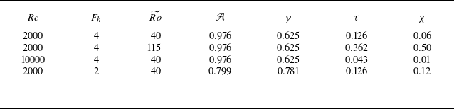
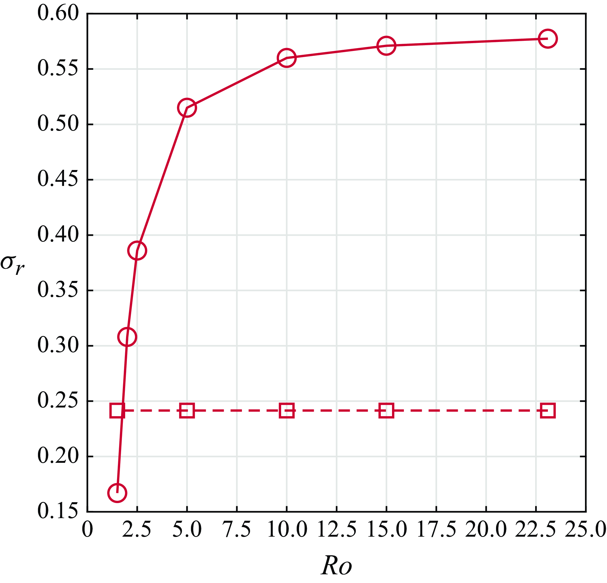
1. Introduction
A common approximation in geophysical fluid dynamics is the traditional approximation that ignores the horizontal component of the planetary rotation when considering a local Cartesian frame at a given latitude. The Coriolis force then takes into account only the vertical component of the planetary rotation. However, as reviewed by Gerkema et al. (Reference Gerkema, Zimmerman, Maas and Van Haren2008), several recent studies examining geophysical flows beyond the traditional approximation suggest that the complete Coriolis force, i.e. with a background rotation along both vertical and horizontal axes, plays a non-negligible role for flows where significant vertical motions or a weak stratification are present. These studies show that the non-traditional Coriolis force generates horizontal asymmetry for horizontally symmetrical flows (Semenova & Slezkin Reference Semenova and Slezkin2003; Sheremet Reference Sheremet2004), modifies and enhances instabilities (Tort, Ribstein & Zeitlin Reference Tort, Ribstein and Zeitlin2016; Zeitlin Reference Zeitlin2018; Park et al. Reference Park, Prat, Mathis and Bugnet2021; Chew, Schlutow & Klein Reference Chew, Schlutow and Klein2023), and changes wave dynamics (Gerkema et al. Reference Gerkema, Zimmerman, Maas and Van Haren2008; Zhang & Yang Reference Zhang and Yang2021). In addition, various models taking into account the complete Coriolis force have been derived (Tort & Dubos Reference Tort and Dubos2014; Tort et al. Reference Tort, Dubos, Bouchut and Zeitlin2014; Lucas, McWilliams & Rousseau Reference Lucas, McWilliams and Rousseau2017).
Toghraei & Billant (Reference Toghraei and Billant2022) have recently studied the evolution of an initially two-dimensional vortex in a stratified fluid under the complete Coriolis force by means of direct numerical simulations (DNS). Due to the horizontal background rotation, a critical layer appears at the radius where the angular velocity of the vortex is equal to the Brunt–Väisälä frequency (i.e. the inverse of the Froude number in non-dimensional form). Such radius exists only if the Froude number is larger than unity. The critical layer induces a vertical velocity field that first grows linearly with time while being more and more concentrated around the critical radius until it finally saturates. Simultaneously, a vertical vorticity anomaly is generated at the critical radius. In parallel to the DNS, Toghraei & Billant (Reference Toghraei and Billant2022) have performed a linear asymptotic analysis for large non-traditional Rossby numbers (based on the horizontal component of the background rotation). It shows that the singularity of the critical layer is smoothed by both viscosity and unsteadiness, like for the baroclinic critical layer in a horizontal shear flow studied by Wang & Balmforth (Reference Wang and Balmforth2020Reference Wang and Balmforth2021). A nonlinear asymptotic analysis has also been conducted following Wang & Balmforth (Reference Wang and Balmforth2020Reference Wang and Balmforth2021) to obtain the velocity and vorticity fields in the critical layer when their amplitude is large. The linear and nonlinear asymptotic solutions for the vertical velocity and the vertical vorticity anomaly have been found to be in excellent agreement with the DNS. Finally, it has been shown that the critical layer generates an inflection point in the vertical vorticity profile that triggers a two-dimensional shear instability for sufficiently high Reynolds numbers and low non-traditional Rossby numbers. A theoretical criterion predicting the occurrence of the two-dimensional instability has been derived from the inflection point condition.
The vortex dynamics described by Toghraei & Billant (Reference Toghraei and Billant2022) is purely two-dimensional but with three velocity components. It can be indeed shown from the governing equations that if the initial conditions are two-dimensional, all the velocity fields remain two-dimensional throughout their evolutions. In the present paper we test the robustness of such evolution with respect to infinitesimal three-dimensional perturbations added at the beginning of the DNS. We will see that the dynamics remains two-dimensional as in Toghraei & Billant (Reference Toghraei and Billant2022) for some parameters, while for other parameters, a three-dimensional instability develops. This newly observed instability resembles the three-dimensional instability reported by Boulanger et al. (Reference Boulanger, Meunier and Le Dizes2007Reference Boulanger, Meunier and Le Dizes2008) in their experimental study of an inclined vortex in a stratified fluid. To some extent, such a configuration is similar to the present one, since in both cases there is a tilt with respect to the gravity force. A critical layer develops in the tilted vortex at the radius where the angular velocity of the vortex is equal to the Brunt–Väisälä frequency and induces an intense vertical velocity field. For a sufficiently large tilt angle and Reynolds number, a three-dimensional instability leads to the formation of rows of vortices with a zig-zag structure. In order to determine the origin of the instability, Boulanger, Meunier & Le Dizes (Reference Boulanger, Meunier and Le Dizes2008) have performed a local stability analysis of the critical layer using the vertical velocity field derived theoretically by means of a linear viscous analysis of the critical layer. Considering only the leading-order terms when the vertical velocity is large, they have shown that the local stability problem reduces to the two-dimensional stability of the vertical velocity field as for the stability of inviscid parallel shear flows. The growth rate predictions obtained by neglecting the azimuthal dependence of the vertical velocity field are in good agreement with the experimentally measured growth rates. Hence, Boulanger et al. (Reference Boulanger, Meunier and Le Dizes2008) have concluded that the three-dimensional instability comes from a shear instability of the vertical velocity field generated in the critical layer. Recently, Wang & Balmforth (Reference Wang and Balmforth2021) have taken a different point of view in their analysis of the two-dimensional shear instability developing within a baroclinic critical layer. They have considered that the instability should be triggered during the initial unsteady regime of the critical layer instead of during the viscous regime as in Boulanger et al. (Reference Boulanger, Meunier and Le Dizes2008). By assuming that the instability arises when the gradient of the vorticity anomaly is of order unity, they have derived an asymptotic model describing the simultaneous development of the base flow in the critical layer and the shear instability. Here, we also follow local approaches in order to determine if the characteristics of the three-dimensional and two-dimensional instabilities can be predicted.
The paper is organised as follows. The initial conditions, governing equations and numerical methods are first presented in § 2. Section 3.1 describes qualitatively the two distinct instabilities observed in DNS when the non-traditional Rossby number is varied while the other parameters are kept constant. Viscous effects are investigated in § 3.2. Linear stability analyses of the flows in the DNS prior to the onset of the instabilities are carried out in § 4. This is completed in § 5 by linear stability analyses of the local theoretical flows in the critical layer. The results of both types of stability analysis are then compared in § 6. Finally, § 7 provides a map of the three-dimensional and two-dimensional instabilities in the parameter space (non-traditional Rossby number, Reynolds number) while § 8 studies the effect of the traditional Rossby number. Conclusions are drawn in § 9.
2. Formulation of the problem
2.1. Initial conditions
A single vertical Lamb–Oseen vortex with vorticity
 \begin{equation} \boldsymbol {\omega } (\boldsymbol x,t=0) = \zeta _0 \boldsymbol {e_z} = \frac {\Gamma }{\pi a_0^2} e^{-r^2/a_0^2} \boldsymbol {e_z}, \end{equation}
where
 $\Gamma$
is the circulation and
 $a_0$
the radius, is considered as initial conditions accompanied by small random three-dimensional perturbations. In the following, we use either Cartesian
 $(x,y,z)$
or cylindrical
 $(r,\theta ,z)$
coordinates. The associated unit vectors are denoted
 $(\boldsymbol {e_x},\boldsymbol {e_y},\boldsymbol {e_z)}$
and
 $(\boldsymbol {e_r},\boldsymbol {e_\theta },\boldsymbol {e_z)}$
, respectively. The geometry of the flow is sketched in figure 1. The vortex is located at the centre of a box with dimensions of
 $l_x \times l_y \times l_z$
. The background rotation vector
 $\boldsymbol {\Omega _b}$
is decomposed into vertical and horizontal components
 $2\boldsymbol {\Omega _b} = \tilde {f} \boldsymbol {e_y} + f \boldsymbol {e_z}$
, where
 $f = 2\Omega _b \sin {(\varphi )}$
and
 $\tilde {f} = 2 \Omega _b \cos {(\varphi )}$
, with
 $\varphi$
the angle between the background rotation vector and the unit vector in the
 $y$
direction,
 $\boldsymbol {e}_y$
. The fluid is stably stratified with a constant Brunt–Väisälä frequency
 $N= \sqrt {-(g/\rho _0) \partial \bar {\rho }/\partial z}$
, where
 $g$
is the gravity,
 $\rho _0$
a constant reference density and
 $\bar {\rho }(z)$
the mean density profile. The velocity field of the small random perturbations consists of a divergence-free white noise with amplitude
 $0.001 \Gamma / 2\pi a_0)$
.
Sketch of the initial vortex in a stratified rotating fluid with a background rotation
 $\Omega _b$
inclined with an angle
 $\varphi$
.

2.2. Governing equations
The initial conditions and governing equations are non-dimensionalised by using
 $2\pi a_0^2/\Gamma$
and
 $a_0$
as time and length units:
 \begin{equation} \boldsymbol {\nabla .u } = 0, \end{equation}
 \begin{equation} \frac {\partial \boldsymbol {u}}{\partial t} + \left ( \boldsymbol {u.\nabla } \right ) \boldsymbol {u} = -\boldsymbol {\nabla }p + b \boldsymbol {e_z} - 2\left ( \frac {1}{Ro} \boldsymbol {e_z} + \frac {1}{\widetilde {Ro}} \boldsymbol {e_y} \right ) \times \boldsymbol {u} + \frac {1}{Re} \boldsymbol {\nabla }^2 \boldsymbol {u}, \end{equation}
 \begin{equation} \frac {\partial b}{\partial t} + \boldsymbol {u.\nabla } b + \frac {1}{F_h^2} u_z = \frac {1}{ReSc} \nabla ^2b. \end{equation}
Here
 $\boldsymbol {u}$
,
 $b$
and
 $p$
are the non-dimensional velocity, buoyancy and pressure, respectively. The problem is controlled by five non-dimensional numbers: the Reynolds, Froude, Rossby and Schmidt numbers defined as
 \begin{equation} Re = \frac {\Gamma }{2\pi \nu }, \quad F_h = \frac {\Gamma }{2\pi a_0^2 N}, \quad Ro = \frac {\Gamma }{\pi a_0^2f}, \quad \widetilde {Ro} = \frac {\Gamma }{\pi a_0^2\tilde {f}}, \quad Sc=\frac {\nu }{\kappa }, \end{equation}
where
 $\nu$
is the viscosity and
 $\kappa$
the diffusivity of the stratifying agent. The two Rossby numbers -- traditional Rossby number
 $Ro$
and non-traditional Rossby number
 $\widetilde {Ro}$
-- measure the two components of the rotation vector. The Schmidt number will always be set to unity. In the following, all the results will be presented in a non-dimensional form.
2.3. Numerical methods
A pseudo-spectral method with periodic boundary conditions and fourth-order Runge–Kutta time integration is used as in Toghraei & Billant (Reference Toghraei and Billant2022). The non-dimensional horizontal sizes of the computational domain have been set to
 $l_x=l_y=18$
to minimise the effect of the periodic boundary conditions (see Toghraei & Billant Reference Toghraei and Billant2022 for details). The vertical size has been set to
 $l_z=8$
in order to accommodate several vertical wavelengths of the dominant three-dimensional instability. The Reynolds number will be varied between
 $Re=2000$
and
 $Re=10000$
. As shown by Toghraei & Billant (Reference Toghraei and Billant2022), the horizontal resolution required for
 $Re=2000$
is
 $n_x=n_y=512$
. Accordingly, the vertical resolution has been set to
 $n_z=256$
. The corresponding time step is
 $\delta t=0.01$
. A number of DNS have been conducted to test the accuracy of the computations. In particular, these tests have shown that the velocity differs by less than
 $ 0.2 \,\%$
when the vertical resolution is increased from
 $n_z=256$
to
 $n_z=512$
. The three-dimensional DNS for higher Reynolds numbers have been performed with a resolution up to
 $n_x=n_y=1536$
,
 $n_z=256$
. Such resolution is sufficient to detect the onset of the three-dimensional instability. However, a study of the nonlinear evolution of the three-dimensional instability could require higher resolution. Two-dimensional DNS have been performed in the range
 $2000 \leqslant Re \leqslant 50000$
with a resolution ranging from
 $n_x=n_y=512$
to
 $n_x=n_y=2048$
.
Vertical velocity field in a horizontal cross-section at
 $z=l_z/2$
(first row) and two vertical cross-sections at
 $y=l_y/2$
(second row) and
 $x=l_x/2$
(third row) at three different times:
 $(a,\!d,\!g)$
 $t = 40$
,
 $(b,\!e,\!h)$
 $t = 53$
,
 $(c,\!f,\!i)$
 $t = 56$
for
 $Re = 2000$
,
 $F_h = 4$
,
 $Ro = 23.1$
and
 $\widetilde {Ro} = 40$
.

Vertical vorticity field in a horizontal cross-section at
 $z=l_z/2$
(first row) and a vertical cross-section at
 $y=l_y/2$
(second row) at three different times: (a,d)
 $t = 40$
, (b,e)
 $t = 53$
, (c,f)
 $t = 56$
for
 $Re = 2000$
,
 $F_h = 4$
,
 $Ro = 23.1$
and
 $\widetilde {Ro} = 40$
.

3. Direct numerical simulations
3.1. Typical examples of the vortex dynamic depending on the non-traditional Rossby number
The objective of this section is to present qualitatively the different vortex evolutions observed in the DNS when the non-traditional Rossby number is varied for a fixed Reynolds number. Figure 2 shows the evolution of the vertical velocity at three different times for the set of parameters
 $Re=2000$
,
 $F_h=4$
,
 $Ro=23.1$
,
 $\widetilde {Ro}=40$
. In this figure, three planes are displayed: a horizontal cross-section at the middle plane
 $z=l_z/2$
(first row) and two vertical cross-sections at the planes
 $y=l_y/2$
(second row) and
 $x=l_x/2$
(third row) going through the initial vortex centre. Figure 3 shows the corresponding evolution of the vertical vorticity. Since the vertical vorticity remains predominantly quasi-asymmetric, only two planes are displayed: a horizontal cross-section in the plane
 $z=l_z/2$
(first row) and a vertical cross-section at the plane
 $y=l_y/2$
(second row).
As previously reported by Toghraei & Billant (Reference Toghraei and Billant2022), the presence of the non-traditional Coriolis force generates a vertical velocity field with azimuthal wavenumber
 $m=1$
(figure 2
 $a{\kern-1pt},{\kern-2pt} d{\kern-1pt},{\kern-2pt}g$
). This vertical velocity field concentrates at the critical radius
 $r_c$
where the non-dimensional angular velocity of the vortex
 $\Omega$
equals the inverse of the Froude number
 $\Omega (r_c) = 1/F_h$
. A ring of vertical vorticity anomaly also develops at
 $r_c$
(figure 3
a,d). The early evolution of these quantities can be seen in Toghraei & Billant (Reference Toghraei and Billant2022). The vortex appears still two-dimensional at
 $t=40$
(figures 2
d,g and 3
d). However, later on (figures 2
b,e,h and 3
b,e), three-dimensional variations become visible in both the vertical velocity and vertical vorticity fields. At
 $t=56$
(figures 2
c,f,i and 3
c,f), the amplitude of the deformations along the vertical has grown and the vertical cross-section of the vertical vorticity (figure 3
f) exhibits a structure similar to that observed by Boulanger et al. (Reference Boulanger, Meunier and Le Dizes2007Reference Boulanger, Meunier and Le Dizes2008) on a stratified tilted vortex. Although there are some irregularities due to the randomness of the initial three-dimensional perturbations, we can distinguish five wavelengths along the vertical, i.e. a dominant wavenumber
 $k\approx 4$
. We can also see that the deformations are in opposite phases on the two sides of the vortex (figure 3
f). In the horizontal cross-sections (figures 2
c and 3
c), non-axisymmetric deformations can also be seen, but they are irregular and weak compared with those of the two-dimensional instability reported by Toghraei & Billant (Reference Toghraei and Billant2022).
In order to prove that the emergence of these three-dimensional disturbances are due to an instability, the vertical vorticity
 $\omega _z$
has been decomposed as
 \begin{equation} \omega _z(x,y,z,t) = \langle \omega _z\rangle _z(x,y,t) + \omega _z'(x,y,z,t), \end{equation}
where
 $ \langle \omega _z\rangle _z=(1/l_z)\int _0^{l_z}\omega _z {\rm d}z$
is the vertically averaged vertical vorticity and
 $ \omega _z'$
three-dimensional fluctuations. Figure 6(a) shows the evolution of the mean square of these two quantities:
 $Z_3=1/V \int _V \langle \omega _z\rangle _z^2 {\rm d}V$
(grey dashed line) and
 $Z_3'=1/V\int _V \omega _z'^2{\rm d}V$
(grey solid line), where
 $V$
is the volume of the computational domain. We can see that, after an initial transient decay,
 $Z_3'$
increases exponentially, indicating the presence of a three-dimensional instability. It then saturates when it reaches the same magnitude as
 $Z_3$
.
A similar three-dimensional instability has been observed when the non-traditional Rossby number is increased to
 $\widetilde {Ro}=60$
(green lines in figure 6
a) or
 $\widetilde {Ro}=80$
(red lines) while keeping the other parameters fixed (see the velocity and vorticity fields in Toghraei Reference Toghraei2023). Note that the corresponding traditional Rossby number
 $Ro$
also varies slightly from
 $Ro=23.1$
to
 $Ro=20.7$
when
 $\widetilde {Ro}$
is increased since it is
 $\varphi$
that is varied whereas
 $\Omega _b=0.1$
is kept constant. As seen in figure 6(a), three-dimensional fluctuations., i.e.
 $Z_3'$
, start to grow exponentially later and with a lower growth rate as
 $\widetilde {Ro}$
increases. Thereby, when the non-traditional Rossby number is further increased to
 $\widetilde {Ro}=115$
(figures 4 and 5), three-dimensional deformations are no longer visible while two-dimensional non-axisymmetric disturbances with an azimuthal mode
 $m=2$
can be seen in the horizontal cross-sections of the vertical vorticity at late times
 $t=167$
and
 $t=175$
(figures 5
b,c), as observed by Toghraei & Billant (Reference Toghraei and Billant2022). Nevertheless, figure 6(a) shows that
 $Z_3'$
still grows exponentially but it remains several orders of magnitude lower than
 $Z_3$
.
Two-dimensional DNS have also been carried out for the same four set of parameters. In this case, the vertical vorticity has been decomposed as
 \begin{equation} \omega _z(r,\theta ,t) = \langle \omega _z\rangle _\theta (r,t)+ \omega _z'(r,\theta ,t), \end{equation}
where
 $ \langle \omega _z\rangle _\theta =1/(2\pi )\int _0^{2\pi }\omega _z {\rm d}\theta$
is the azimuthally averaged vertical vorticity and
 $\omega _z'$
non-axisymmetric fluctuations. Figure 6(b) displays the evolution of
 $Z_2=1/S \int _S \langle \omega _z\rangle _\theta ^2 {\rm d}S$
(grey dashed line) and
 $Z_2'=1/S\int _S \omega _z'^2{\rm d}S$
(grey solid line), where
 $S$
is the surface of the domain. Again, we can see that non-axisymmetric fluctuations, i.e.
 $Z_2'$
, grow exponentially for the four values of
 $\widetilde {Ro}$
owing to the two-dimensional instability studied previously by Toghraei & Billant (Reference Toghraei and Billant2022). Yet, in the full three-dimensional configuration, it is only for
 $\widetilde {Ro}=115$
that the two-dimensional instability is observed. There is therefore a competition between two different instabilities and the nature of the dominant instability depends on the parameters. We can notice that the maximum vertical velocity is larger by
 $50\,\%$
for
 $\widetilde {Ro}=40$
(figure 2
a,d,g) than for
 $\widetilde {Ro}=115$
(figures 4
a,d,g). However, the vertical vorticity anomaly is much stronger for
 $\widetilde {Ro}=40$
(figure 3
a,d) than for
 $\widetilde {Ro}=115$
(figure 5
a,d), so that the type of dominant instability cannot be guessed by simply looking at the vertical velocity and vorticity profiles.
Same as figure 2 but for
 $\widetilde {Ro} = 115$
and
 $Ro = 20.3$
:
 $(a,\!d,\!g)$
 $t = 100$
, (b,e,h)
 $t = 152$
, (c,f,i)
 $t = 167$
.

Same as figure 3 but for
 $\widetilde {Ro} = 115$
and
 $Ro = 20.3$
: (a,d)
 $t = 100$
, (b,e)
 $t = 152$
, (c,f)
 $t = 167$
.

(a) Evolution of the mean square of the vertically averaged vertical vorticity
 $Z_3$
(dashed lines) and of the three-dimensional vertical vorticity fluctuations
 $Z_3^{\prime}$
(solid lines) in three-dimensional DNS. (b) Evolution of the mean square of the azimuthally averaged vertical vorticity
 $Z_2$
(dashed lines) and of the non-axisymmetric vertical vorticity fluctuations
 $Z_2^{\prime}$
(solid lines) in two-dimensional DNS. The parameters are
 $\widetilde {Ro} = 40$
(grey lines),
 $\widetilde {Ro} = 60$
(green lines),
 $\widetilde {Ro} = 80$
(red lines),
 $\widetilde {Ro} = 115$
(blue lines) for
 $Re = 2000$
,
 $F_h = 4$
and
 $\Omega _b=0.1$
(
 $Ro \approx 20$
). The straight solid lines indicate the slopes for each
 $\widetilde {Ro}$
corresponding to the dominant three-dimensional growth rate in (a) and to the growth rate at
 $k=0$
in (b) for the last time
 $t_b$
investigated in the linear stability analyses of the DNS flows (figure 11). In (a) the blue straight dashed line represents the slope corresponding to the growth rate at
 $k=0$
for
 $\widetilde {Ro} = 115$
.

3.2. Viscous and diffusion effects
In order to study viscous and diffusion effects, we conducted three series of three-dimensional DNS for different Reynolds numbers between
 $Re=2000$
and
 $Re=10000$
. The first series has been conducted for a constant non-traditional Rossby number
 $\widetilde {Ro}=80$
, whereas the second and third series have been performed for a constant value of
 $\varepsilon ^2 Re$
or
 $\varepsilon Re^{2/3}$
, where
 $\varepsilon =2/\widetilde {Ro}$
. These combinations of
 $\widetilde {Ro}$
and
 $Re$
correspond to the typical amplitudes of the vorticity anomaly in the critical layer and of the gradient of the vertical velocity in the critical layer when viscous effects operate, respectively (see § 5.1 below and Toghraei & Billant Reference Toghraei and Billant2022). These three series allow us to explore different regions of the parameter space (
 $Re,\widetilde {Ro}$
). The DNS for
 $\widetilde {Ro}=80$
and
 $Re=2000$
belongs to the three series and is therefore the reference.
Figure 7(a) shows that, for constant
 $\widetilde {Ro}=80$
, three-dimensional vertical vorticity fluctuations,
 $Z_3'$
, grow exponentially earlier and with a larger growth rate when the Reynolds number is increased from
 $Re=2000$
to
 $Re=4000$
. However, for higher values of
 $Re$
, the growth rate remains almost constant (the growth rate as a function of
 $Re$
is also shown in figure 8
b by blue open circles). As seen in figure 8(a), the observed dominant vertical wavenumber (blue open circles) first increases with
 $Re^{1/3}$
and then remains constant. For a constant value of
 $\varepsilon ^2 Re$
(figure 7
b) or
 $\varepsilon Re^{2/3}$
(figure 7
c), the exponential growth rate of
 $Z_3'$
is approximately independent of the Reynolds number (see also the green and red open circles in figure 8
b). In contrast, the dominant vertical wavenumber (green and red open circles in figure 8
a) seems to increase linearly with
 $Re^{1/3}$
(green dashed line) both for
 $\varepsilon ^2 Re=1.25$
and
 $\varepsilon Re^{2/3}=3.97$
, as observed by Boulanger et al. (Reference Boulanger, Meunier and Le Dizes2008). The increase of the wavenumber is also directly visible in the vertical cross-sections of the vertical vorticity displayed in figure 9 for
 $\varepsilon Re^{2/3}=3.97$
. This observation will be the basis of one of the assumption of the local asymptotic three-dimensional stability analysis performed in § 5.
Similarly, the effect of the Reynolds number on the two-dimensional instability has been studied by performing two-dimensional DNS for different Reynolds numbers between
 $Re=2000$
and
 $Re=50000$
for
 $\widetilde {Ro}=80$
and for a constant value of
 $\varepsilon ^2 Re=1.25$
or
 $\varepsilon Re^{2/3}=3.97$
. When
 $\widetilde {Ro}=80$
, figure 10(a) shows that non-axisymmetric vertical vorticity fluctuations
 $Z_2'$
start to grow exponentially earlier when
 $Re$
is increased from
 $Re=2000$
to
 $Re=6000$
. However, for
 $6000 \leqslant Re \leqslant 50000$
, the two-dimensional instability always starts to be amplified around
 $t=75$
and its growth rate becomes approximately independent of
 $Re$
. In contrast, when
 $\varepsilon ^2 Re$
is kept constant (figure 10
b),
 $Z_2^{\prime}$
starts to grow exponentially later and later as
 $Re$
is increased from
 $Re=2000$
to
 $Re=50000$
. The growth rate remains approximately the same and the instability always exhibits an azimuthal wavenumber
 $m=2$
for all these two-dimensional DNS. Similar trends are observed for
 $\varepsilon Re^{2/3}=3.97$
when
 $Re$
is increased from
 $Re=2000$
to
 $Re=10000$
(figure 10
c).
Evolution of the mean square of the vertically averaged vertical vorticity
 $Z_3$
(dashed lines) and of the three-dimensional vertical vorticity fluctuations
 $Z_3^{\prime}$
(solid lines) in three-dimensional DNS for different Reynolds numbers for (a)
 $\widetilde {Ro} = 80$
, (b)
 $\varepsilon ^2 Re=1.25$
, (c)
 $\varepsilon Re^{2/3}=3.97$
for
 $F_h = 4$
and
 $\Omega _b=0.1$
(
 $Ro \approx 20$
). The Reynolds numbers are
 $Re = 2000$
(green line),
 $Re = 4000$
(red line),
 $Re = 6000$
(blue line),
 $Re = 8000$
(grey line),
 $Re = 10000$
(black line). The square symbols indicate the time
 $t_b$
considered in the stability analyses.

(a) Most amplified vertical wavenumber
 $k$
as a function of
 $Re^{1/3}$
. (b) Associated maximum growth rate as a function of
 $Re$
. The blue, red and green symbols correspond to
 $\widetilde {Ro} = 80$
,
 $\varepsilon ^2 Re=1.25$
and
 $\varepsilon Re^{2/3}=3.97$
, respectively, for
 $F_h = 4$
and
 $\Omega _b=0.1$
(
 $Ro \approx 20$
). The symbols
 $\circ$
,
 $\times$
and
 $+$
represent the results obtained from the DNS and from the local three-dimensional stability analyses of the linear solution (5.1, 5.4, 5.6) and nonlinear solution (5.1, 5.3), respectively. In (a) the green dashed line shows a linear fit of the green and red circle symbols. The time
 $t_b$
taken for each local stability analysis of the DNS flow is indicated in figure 7.

Vertical vorticity field in a vertical cross-section at
 $y=l_y/2$
for
 $\varepsilon Re^{2/3}=3.97$
for (a) (
 $Re = 2000$
,
 $\widetilde {Ro} = 80$
,
 $t=102$
), (b) (
 $Re = 4000$
,
 $\widetilde {Ro} = 127$
,
 $t=100$
), (c) (
 $Re = 6000$
,
 $\widetilde {Ro} = 167$
,
 $t=104$
) and (d) (
 $Re = 10000$
,
 $\widetilde {Ro} = 223.8$
,
 $t=104$
) for
 $F_h = 4$
and
 $\Omega _b=0.1$
(
 $Ro \approx 20$
).

Evolution of the mean square of the azimuthally averaged vertical vorticity
 $Z_2$
(dashed lines) and of the non-axisymmetric vertical vorticity fluctuations
 $Z_2^{\prime}$
(solid lines) in two-dimensional DNS for different Reynolds numbers for (a)
 $\widetilde {Ro} = 80$
, (b)
 $\varepsilon ^2 Re=1.25$
and (c)
 $\varepsilon Re^{2/3}=3.97$
for
 $F_h = 4$
and
 $\Omega _b=0.1$
(
 $Ro \approx 20$
). The Reynolds numbers are
 $Re = 2000$
(green line),
 $Re = 4000$
(red line),
 $Re = 6000$
(dark blue line),
 $Re = 8000$
(grey line),
 $Re = 10000$
(black line),
 $Re = 20000$
(orange line),
 $Re = 30000$
(light blue line),
 $Re = 50000$
(dark yellow line). The square symbols indicate the time
 $t_b$
considered in the stability analyses.

4. Linear stability analysis of the flows in the DNS
In order to further describe the competition between the two-dimensional and three-dimensional instabilities, we have carried out linear stability analyses of the flows in the DNS at different times before the onset of the instability.
4.1. Methods
To do so, the velocity and buoyancy fields
 $\boldsymbol {U}=(U_x,U_y,U_z)$
and
 $B$
have been frozen at a given time
 $t=t_b$
. These base flows have been extracted from the two-dimensional simulations. This ensures they are not disturbed by any instability since the simulations are two-dimensional and the two-dimensional instability develops later than the time
 $t_b$
under consideration. They are next perturbed by infinitesimal perturbations
 \begin{equation} [\boldsymbol {u},b] (\boldsymbol {x},t) = [\boldsymbol {U},B] (x,y,t_b) + [\boldsymbol {u}^{\prime },b^{\prime }] (\boldsymbol {x},t), \end{equation}
denoted with a prime. The perturbations are governed by the equations (2.2–2.4) linearised around
 $(\boldsymbol {U},B)$
:
 \begin{equation} {\boldsymbol {\nabla .u}}^{\prime} = 0, \end{equation}
 \begin{equation} \frac {\partial {{\boldsymbol u}^{\prime }}}{\partial t} + \left ( \boldsymbol {U.\nabla } \right ) {\boldsymbol u}^{\prime} + \left ({\boldsymbol u}^{\prime}.{\boldsymbol \nabla} \right ) \boldsymbol {U}= -\boldsymbol {\nabla }p^{\prime } + b^{\prime } \boldsymbol {e_z} - 2\left ( \frac {1}{Ro} \boldsymbol {e_z} + \frac {1}{\widetilde {Ro}} \boldsymbol {e_y} \right ) \times {\boldsymbol u}^{\prime} + \frac {1}{Re} \boldsymbol {\nabla }^2 {\boldsymbol u}^{\prime}, \end{equation}
 \begin{equation} \frac {\partial b^{\prime }}{\partial t} + \boldsymbol {U.\nabla } b^{\prime } + \boldsymbol {u^{\prime }.\nabla } B + \frac {1}{F_h^2} u_z^{\prime } = \frac {1}{ReSc} \nabla ^2b^{\prime }. \end{equation}
Such a ‘freezing’ method is expected to give reliable results if the time evolution of the flow
 $(\boldsymbol {U},B)$
is slow compared with the growth rate of the perturbations.
The equations (4.2–4.4) are integrated with
 $[\boldsymbol {u^{\prime }},b^{\prime }]$
initialised by white noise using the same numerical code and the same resolution and domain size in the horizontal directions as for the DNS. Since the base flow
 $(\boldsymbol {U},B)$
is uniform along the vertical and the equations (4.2–4.4) are linear, the amplitude
 $[\boldsymbol {\hat {u}_k},\hat {b}_k]$
of each vertical wavenumber of the perturbation
 \begin{equation} [\boldsymbol {u^{\prime }},b^{\prime }] = \sum _{k=-k_{max}}^{k_{max}} [\boldsymbol {\hat {u}_k},\hat {b}_k] (x,y,t)\mathrm {e}^{\mathrm {i}kz} \end{equation}
evolve independently of the others. Hence, by integrating (4.2–4.4) for a sufficiently long time, the perturbations
 $[\boldsymbol {\hat {u}_k},\hat {b}_k]$
will be dominated by the most unstable mode for the vertical wavenumber
 $k$
. The vertical size and resolution have been set to
 $l_z=32$
and
 $n_z=64$
in order to cover the wavenumber band
 $-2\pi \leqslant k \leqslant 2\pi$
with the resolution
 $\Delta k = \pi / 16$
.
In practice, the growth rate for each vertical wavenumber
 $\sigma _r (k)$
is retrieved from the total kinetic energy
 $E_k(t)=\int \int 1/2 ( \hat {u}_x^2+\hat {u}_y^2+\hat {u}_z^2 ) \mathrm {d}x \mathrm {d}y$
by means of the formula
 \begin{equation} \sigma _r (k) = \frac {1}{2(t_f-t_i)} \log \left ( \frac {E_k (t_f)}{E_k (t_i)} \right ), \end{equation}
where the two times
 $t_i$
and
 $t_f$
are chosen to be large and sufficiently separated in order to eliminate the oscillations of
 $E_k$
when the instability is oscillating (typically,
 $t_i=140$
and
 $t_f=190$
). The frequency
 $\sigma _i(k)$
of the instability can also be retrieved by searching the successive times
 $t_n$
for which the relative kinetic energy
 $E_k(t)/(E_k(t_i)\mathrm {e}^{2\sigma _r(t-t_i)})$
is maximum. An estimation of the frequency is then given by
 \begin{equation} \sigma _i (k) = \frac {1}{(n_{max}-1)}\sum _{n=1}^{n_{max}-1} \frac {2 \pi }{2(t_{n+1}-t_n)}, \end{equation}
where
 $n_{max}$
is the number of maxima detected. In the following, only positive wavenumbers
 $k$
will be presented since negative ones are identical owing to the symmetry
 $z \rightarrow -z$
.
Growth rate
 $\sigma _r$
obtained from the stability analysis of the DNS flow as a function of the vertical wavenumber
 $k$
for
 $\textrm {Re} = 2000$
,
 $F_h=4$
,
 $\Omega _b=0.1$
(
 $Ro \approx 20$
) and (a)
 $\widetilde {Ro} = 40$
, (b)
 $\widetilde {Ro} = 60$
, (c)
 $\widetilde {Ro} = 80$
and (d)
 $\widetilde {Ro} = 115$
. The coloured lines correspond to different times
 $t_b$
: (a)
 $t_b = 35$
(black line),
 $t_b = 40$
(green line),
 $t_b = 45$
(red line),
 $t_b = 50$
(blue line); (b)
 $t_b = 40$
(black line),
 $t_b = 50$
(green line),
 $t_b = 55$
(red line),
 $t_b = 60$
(blue line); (c)
 $t_b = 45$
(black line),
 $t_b = 55$
(green line),
 $t_b = 65$
(red line),
 $t_b = 75$
(blue line), (d)
 $t_b = 50$
(black line),
 $t_b = 70$
(green line),
 $t_b = 90$
(red line),
 $t_b = 100$
(blue line).

4.2. Results for variable non-traditional Rossby number
Figure 11 shows the growth rate as a function of the vertical wavenumber
 $k$
for the four different values of
 $\widetilde {Ro}$
investigated in § 3.1 for
 $Re=2000$
and
 $F_h=4$
. For each case, we computed the stability of the flows at four different times
 $t_b$
prior to the time at which the instabilities become visible in the DNS. We remind the reader that the base flows have been extracted from two-dimensional simulations in which no three-dimensional instability occurs. The curves are not smooth and exhibit some small irregularities because there are several subdominant modes with a growth rate close to that of the dominant modes. The convergence towards the dominant mode with the present method is therefore slow and still not perfect between the integration time
 $t_i$
and
 $t_f$
. It is however sufficiently converged for the present purpose. Globally, the growth rate levels increase with
 $t_b$
and decrease with
 $\widetilde {Ro}$
. For
 $\widetilde {Ro}=40$
(figure 11
a), all the wavenumbers are strongly unstable but there is a growth rate peak at
 $k\approx 4-5$
in agreement with the dominant wavenumber
 $k\approx 4$
observed in the DNS (figures 2 and 3). Figure 12(a) shows the frequency
 $\sigma _i$
corresponding to this peak (circle symbols) as a function of
 $t_b$
. It is nearly constant,
 $\sigma _i \approx 0.2$
, when
 $t_b \geqslant 40$
and clearly differs from the frequency of the two-dimensional instability (i.e. for
 $k=0$
), which is also plotted with square symbols. The vertical velocity and vertical vorticity of the eigenmodes corresponding to the dominant three-dimensional instability and to the two-dimensional instability also have a different structure (figure 13) even if they are both concentrated around the critical radius. The vertical vorticity of the two-dimensional eigenmode (figure 13
c) exhibits a well-defined azimuthal wavenumber,
 $m=3$
, that rotates with little shape change. This wavenumber is less clear in the vertical velocity (figure 13
a) since the base vertical velocity is non-axisymmetric. Nevertheless, there are also six extrema along a circular path even if their amplitude is irregular. In contrast, the three-dimensional eigenmode (figure 13
b,d) presents an irregular azimuthal dependence that is modulated over the oscillation period of the instability.
Frequency
 $\sigma _i$
obtained from the stability analysis of the DNS flow for
 $k=0$
(squares) and at the most amplified wavenumber in the range
 $k\gt 4$
(circles) as a function of the time
 $t_b$
for
 $\textrm {Re} = 2000$
,
 $F_h=4$
,
 $\Omega _b=0.1$
(
 $Ro \approx 20$
) and (a)
 $\widetilde {Ro} = 40$
, (b)
 $\widetilde {Ro} = 60$
, (c)
 $\widetilde {Ro} = 80$
and (d)
 $\widetilde {Ro} = 115$
.

Vertical velocity (a,b) and vertical vorticity (c,d) of the eigenmode for (a,c)
 $k=0$
and
 $(b,d)k=4.5$
for
 $\widetilde {Ro} = 40$
and
 $Re = 2000$
,
 $F_h = 4$
,
 $Ro = 23.1$
at
 $t_b = 50$
.

As the non-traditional Rossby number is increased to
 $\widetilde {Ro}=60$
(figure 11
b) and
 $\widetilde {Ro}=80$
(figure 11
c), a peak continues to be observed around
 $k\approx 4-5$
but it is less pronounced relative to the growth rate at
 $k=0$
. In other words, the three-dimensional instability is still dominant for these values of
 $\widetilde {Ro}$
as observed in the DNS but its strength weakens comparatively to the two-dimensional instability. The frequency corresponding to the growth rate peak is still around
 $\sigma _i \approx 0.2$
(figure 12
b,c). However, the frequency of the two-dimensional instability switches from
 $\sigma _i \approx 0.5$
at early times to
 $\sigma _i \approx 0.8$
at late times.
For
 $\widetilde {Ro}=115$
(figure 11
d), the growth rate is maximum at
 $k=0$
, in agreement with the observation of a two-dimensional instability in the DNS (figures 4 and 5). A local peak around
 $k\approx 4-5$
is however still observed when
 $t_b \leqslant 80$
, whereas it is less apparent for
 $t_b \geqslant 100$
. The present linear stability analysis, therefore, confirms that there is a cross-over of the dominant instability from three-dimensional to two-dimensional as
 $\widetilde {Ro}$
increases. As seen in figure 12(d), the frequencies of the three-dimensional and two-dimensional instabilities are now
 $\sigma _i \approx 0.2$
and
 $\sigma _i \approx 0.5$
, respectively, independently of
 $t_b$
. Interestingly, figure 14(c) shows that the vertical vorticity of the eigenmode of the two-dimensional instability exhibits now a
 $m=2$
azimuthal structure, as observed in the DNS (figures 4 and 5), instead of
 $m=3$
for
 $\widetilde {Ro}=40$
(figure 13
c). This change of the dominant azimuthal wavenumber of the two-dimensional instability explains why the frequency switches from
 $\sigma _i \approx 0.8$
for
 $\widetilde {Ro}=40$
to
 $\sigma _i \approx 2/3 \times 0.8 \approx 0.5$
for
 $\widetilde {Ro}=115$
. The three-dimensional eigenmode for
 $\widetilde {Ro}=115$
(figure 14
b) looks somewhat different from the one for
 $\widetilde {Ro}=40$
(figure 13
b) because they do not correspond to the same phase of the oscillation cycle.
Although the stability analysis has been performed by freezing a time-evolving flow
 $[\boldsymbol {U},B]$
, we note in figure 11 that the growth rate curves for the two last times
 $t_b$
(red and blue lines) are very close for each plot. This indirectly suggests that the flow
 $[\boldsymbol {U},B]$
has little evolved between these two times. The slow evolution of the base flow
 $[\boldsymbol {U},B]$
when the instability develops will be confirmed in the next section.
Finally, the exponential growth corresponding to the dominant three-dimensional growth rate obtained in the linear stability analyses at the last time
 $t_b$
(figure 11) are indicated by straight solid lines for each
 $\widetilde {Ro}$
in figure 6
 $(a)$
. We see that the slopes compare very well with those observed in the DNS, except for
 $\widetilde {Ro}=115$
. In this case, the slope corresponds more to the growth rate for
 $k=0$
indicated by a blue straight dashed line, consistently with the observation of a two-dimensional instability. Similarly, figure 6
 $(b)$
shows that the slopes of the exponential growth in the two-dimensional DNS for each
 $\widetilde {Ro}$
are in very good agreement with the growth rate for
 $k=0$
obtained from the linear stability analyses at the last time
 $t_b$
(figure 11).
Same as figure 13 but for
 $(a,c)$
 $k=0$
and
 $(b,d)$
 $k=5.3$
for
 $\widetilde {Ro} = 115$
and
 $Ro=20.3$
at
 $t_b = 100$
.

(a) Most amplified azimuthal wavenumber
 $m$
as a function of
 $Re^{1/3}$
. (b) Associated maximum growth rate as a function of
 $Re$
. The blue, red and green symbols correspond to
 $\widetilde {Ro} = 80$
,
 $\varepsilon ^2 Re=1.25$
and
 $\varepsilon Re^{2/3}=3.97$
, respectively, for
 $F_h = 4$
and
 $\Omega _b=0.1$
(
 $Ro \approx 20$
). The symbols
 $\circ$
,
 $\times$
and
 $+$
represent the results obtained from linear stability analyses of the DNS flows and from the local two-dimensional stability analyses of the linear solution (5.1, 5.4, 5.6) and nonlinear solution (5.1, 5.3), respectively. In (a) the red dashed line shows a linear fit of the red open circle symbols (
 $\circ$
). The time
 $t_b$
taken for each stability analysis of the DNS flow and local stability analyses is indicated in figure 10. For green symbols with
 $Re \gt 10000$
, the base flows in the local stability analyses have been taken at
 $t_b$
=
 $6Re^{1/3}$
.

4.3. Results for variable Reynolds number in the two-dimensional case
The two-dimensional linear stability of the two-dimensional DNS flows for different
 $Re$
(§ 3.2) have also been investigated. Several Reynolds numbers in the range
 $2000 \leqslant Re \leqslant 50000$
have been studied both for
 $\widetilde {Ro}=80$
and for a constant value of
 $\varepsilon ^2 Re=1.25$
or
 $\varepsilon Re^{2/3}=3.97$
. The time
 $t_b$
considered for each case is indicated by a symbol in figure 10. These analyses reveal that the azimuthal wavenumber
 $m=2$
is not the most unstable one for large Reynolds numbers even if the corresponding two-dimensional DNS always exhibit an azimuthal wavenumber
 $m=2$
whatever
 $\widetilde {Re}$
and
 $\widetilde {Ro}$
in the ranges investigated. Indeed, figure 15(a) shows that the most unstable azimuthal wavenumber for
 $\widetilde {Ro}=80$
(blue open circles) first increases from
 $m=3$
for
 $Re^{1/3}=13$
(i.e.
 $Re=2000$
) to
 $m=8$
for
 $Re^{1/3}=27$
(
 $Re=20000$
) but tends to remain constant for higher values of
 $Re^{1/3}$
. For fixed
 $\varepsilon ^2 Re$
,
 $m$
increases continuously with
 $Re^{1/3}$
up to
 $m=6$
for
 $Re^{1/3}=37$
(
 $Re=50000$
) (red open circles in figure 15
a). The red dashed line in figure 15(a) shows that the azimuthal wavenumber
 $m$
in the latter case varies approximately linearly with
 $Re^{1/3}$
. The corresponding maximum growth rate first increases with
 $Re$
for
 $\widetilde {Ro}=80$
and then tends to saturate (blue open circles in figure 15
b), whereas it remains approximately constant when
 $\varepsilon ^2 Re=1.25$
is kept fixed (red open circles). In contrast, for
 $\varepsilon Re^{2/3}=3.97$
(green open circles), the azimuthal wavenumber remains
 $m=3$
and the growth rate decreases when
 $Re$
is varied from
 $Re^{1/3}=13$
(
 $Re=2000$
) to
 $Re^{1/3}=21$
(
 $Re=10000$
).
The three-dimensional stability of flows in the DNS for variable Reynolds numbers has not been investigated, as knowledge of the maximum growth rate and dominant wavenumber extracted from the DNS will be sufficient in the remainder of the study.
5. Local stability analysis of the theoretical solutions in the critical layer
In order to shed light on the mechanism and competition between the three-dimensional and two-dimensional instabilities, we now turn to a stability analysis of the local solutions in the critical layer that have been derived analytically for large Reynolds numbers and small non-traditional Rossby numbers in Toghraei & Billant (Reference Toghraei and Billant2022).
We first briefly recall the asymptotic analyses and the resulting solutions. Then, the stability of these solutions will be investigated.
5.1. Local base flow in the critical layer
This section is only a brief summary of the main asymptotic results derived in Toghraei & Billant (Reference Toghraei and Billant2022) that will be useful in the next sections; readers interested in the details of the asymptotic analyses are referred to this paper. Toghraei & Billant (Reference Toghraei and Billant2022) have solved (2.2–2.4) by assuming
 $\varepsilon = 2/\widetilde {Ro} \ll 1$
and
 $Re \gg 1$
and by considering the vicinity of the critical radius
 $r_c$
where
 $\Omega (r_c) = 1/F_h$
by means of the variable
 $\tilde {r} = Re ^{1/3}(r-r_c)$
. A slow time
 $T=Re^{-1/3}t$
has also been introduced. Both linear and nonlinear analyses have been carried out following Boulanger, Meunier & Le Dizes (Reference Boulanger, Meunier and Le Dizes2007) and Wang & Balmforth (Reference Wang and Balmforth2020). The nonlinear analysis assumes the distinguished scaling
 $Re=\widetilde {Re}/\varepsilon ^2$
where
 $\widetilde {Re}$
is of order unity. However, the nonlinear analysis remains valid for any value in the range
 $0 \lt \widetilde {Re} \lt 1$
and recovers the linear analysis in the limit
 $\widetilde {Re} \to 0$
. The solutions for the vertical velocity, buoyancy, angular velocity and vertical vorticity then read, at leading order in
 $\varepsilon$
,
 \begin{equation} U_{z} = \varepsilon ^{1/3} \widetilde {Re}^{1/3} \tilde {U}_{z} + \ldots , \end{equation}
 \begin{equation} B =\varepsilon ^{1/3} \widetilde {Re}^{1/3} \tilde {B} + \ldots , \end{equation}
 \begin{equation} \Omega = \Omega _0 + \varepsilon ^{2/3} \widetilde {Re}^{2/3} \Omega _1 + \ldots , \end{equation}
 \begin{equation} \zeta = \zeta _0 + \widetilde {Re} \zeta _1 + \ldots , \end{equation}
where
 $\tilde {U}_{z} = \tilde {U}_{z1} \mathrm {e}^{ \mathrm {i} \theta } + c.c.$
and
 $\tilde {B} = \tilde {B}_1 \mathrm {e}^{\mathrm {i} \theta } + c.c.$
. At the leading order,
 $\Omega _0$
and
 $\zeta _0$
are the non-dimensional angular velocity and vertical vorticity corresponding to (2.1). In the vicinity of
 $r_c$
, they can be expanded as
 \begin{equation} \Omega _0 =\Omega _c + \tilde {r} \Omega _c^{\prime } \varepsilon ^{2/3} \widetilde {Re}^{-1/3} + \ldots , \end{equation}
 \begin{equation} \zeta _0 =\zeta _c + \tilde {r} \zeta _c^{\prime } \varepsilon ^{2/3} \widetilde {Re}^{-1/3} + \ldots , \end{equation}
where the subscript
 $c$
denotes the value at
 $r=r_c$
. The vertical velocity
 $\tilde {U}_{z1}$
and angular velocity correction
 $\Omega _1$
have been found to be governed by the following coupled equations:
 \begin{equation} \frac {\partial \tilde {U}_{z1}}{\partial T} + \mathrm {i} \Omega _c^{\prime }\tilde {r} \tilde {U}_{z1} + \mathrm {i} \widetilde {Re} \Omega _1 \tilde {U}_{z1} = \frac {\mathrm {i}}{4}r_c \Omega _c + \frac {1}{2} \left (1 + \frac {1}{Sc} \right ) \frac {\partial ^{2}\tilde {U}_{z1}}{\partial \tilde {r}^2}, \end{equation}
 \begin{equation} \frac {\partial \Omega _{1}}{\partial T} = - \frac {\mathrm {i}}{2r_c} \left ( \tilde {U}_{z1}^{*} - \tilde {U}_{z1} \right ) + \frac {\partial ^2 \Omega _1}{\partial \tilde {r}^2}. \end{equation}
Equation (5.3a
) describes the evolution of the vertical velocity
 $\tilde {U}_{z1}$
near
 $r_c$
due to the non-traditional Coriolis force (first term on the right-hand side) and under the viscous and diffusive effects (last term on the right-hand side) and the effect of the angular velocity correction
 $\Omega _1$
(last term on the left-hand side). The viscous effects and the time derivative smooth the solution
 $\tilde {U}_{z1}$
, which without these terms would be
 $\tilde {U}_{z1} = r_c \Omega _c / (4 \Omega _c^{\prime }\tilde {r})$
and would be therefore singular at
 $r_c$
. Equation (5.3b
) shows that the vertical velocity
 $\tilde {U}_{z1}$
forces the angular velocity correction
 $\Omega _1$
. This comes from the non-traditional Coriolis force in the horizontal momentum equation. The corresponding buoyancy and vertical vorticity corrections are given by
 $\tilde {B}_1 = i \Omega _c \tilde {U}_{z1}$
and
 $\zeta _1 = r_c \partial \Omega _1 / \partial \tilde {r}$
. Note that the parameter
 $\widetilde {Re}$
does not appear in the viscous terms but instead in front of the nonlinear term in (5.3a
) because
 $\widetilde {Re}$
has been included in the expansions (5.1), whereas they were expressed only in terms of
 $\varepsilon$
in the nonlinear analysis of Toghraei & Billant (Reference Toghraei and Billant2022). The advantage of taking into account
 $\widetilde {Re}$
in (5.1) is that the same expansions can be used in the linear and nonlinear cases.
The linear solutions derived by Toghraei & Billant (Reference Toghraei and Billant2022) correspond to the case when the angular velocity correction is small so that its retroaction on the vertical velocity is negligible. This linear limit can be most simply obtained from (5.3) by neglecting the third term on the left-hand side of (5.3a
). Indeed, the linear solutions are expected to be valid when the vertical vorticity correction
 $\widetilde {Re}\zeta _1$
in (5.1d
) is weak, i.e. when
 $\widetilde {Re} \ll 1$
, or equivalently,
 $Re/ \widetilde {Ro}^2 \ll 1$
. In this case, (5.3a
) can be integrated to give
 \begin{equation} \tilde {U}_{z1} = \mathrm {i} \frac {\mathcal {A} }{\pi } \int _0^{\big |{\Omega _c^{\prime }}\big |T/ \gamma } \mathrm {exp} \left ( - \frac {z^3}{3} + \mathrm {i} \gamma \tilde {r} z \right ) \mathrm {d}z, \end{equation}
where
 \begin{equation} \mathcal {A} ={\frac { \pi r_c \Omega _c}{ 2 \big |{2\Omega _c^{\prime }}\big |^{2/3}\left (1+\frac {1}{Sc}\right )^{1/3}}}, \qquad \gamma = {\frac { \big |{2\Omega _c^{\prime }}\big |^{1/3}}{ \left (1+\frac {1}{Sc}\right )^{1/3}}}. \end{equation}
Then, the solution of (5.3b ) can be found in the form
 \begin{equation} \Omega _{1} = - \frac { \mathcal {A}}{2\gamma ^2\pi r_c} \int _0^{\big |{\Omega _c^{\prime }}\big |T/\gamma }\! \mathrm {exp} \left (\! \frac {-z^3}{3} + \mathrm {i}\gamma \tilde {r} z \!\right ) \left ( \!\frac {1-\mathrm {exp}\left ( \gamma ^3 z^3/\big |{\Omega _c^{\prime }}\big | - \gamma ^2 z^2T \!\right )}{z^2} \right ) \mathrm {d}z + c.c. \end{equation}
The theoretical solutions (5.3), (5.4) and (5.6) have been computed numerically and are compared in figure 16 to the flows observed in the three-dimensional DNS prior to the onset of the instability for the four values of
 $\widetilde {Ro}$
investigated previously for
 $Re=2000$
and
 $F_h=4$
. This figure displays the maximum vertical velocity
 $U_{zm}(\theta ,t)$
for
 $\theta =0$
(figure 16
a) and
 $\theta =\pi /2$
(figure 16
b). The solid lines correspond to the DNS for
 $\widetilde {Ro}=40$
(grey),
 $\widetilde {Ro}=60$
(green),
 $\widetilde {Ro}=80$
(red) and
 $\widetilde {Ro}=115$
(blue), whereas the corresponding linear (5.1, 5.4) and nonlinear (5.1, 5.3) solutions are plotted with dashed lines and dotted-dashed lines, respectively, with the same colour.
Both the linear (5.1, 5.4) and nonlinear (5.1, 5.3) solutions predict well the initial increase of
 $U_{zm}(\theta ,t)$
in the DNS for all values of
 $\widetilde {Ro}$
despite missing the initial oscillations observed in the DNS. These oscillations are due to inertia-gravity waves excited at
 $t=0$
. However, since their amplitude remains constant whereas the rest of the solution grows linearly with time, their relative importance becomes negligible for large times. They are absent in (5.3) and (5.4) because these solutions are valid only for
 $T \gtrsim \mathcal {O}(1)$
, i.e. large time:
 $t \gg \varepsilon ^{-2/3} \widetilde {Re}^{1/3}$
.
Comparison between the maximum vertical velocity in the DNS (solid line), predicted by the linear solution (5.1, 5.4) (dashed line) and by the nonlinear equations (5.1, 5.3) (dotted-dashed line) for (a)
 $\theta =0$
and (b)
 $\theta =\pi /2$
for
 $Re=2000$
,
 $F_h=4$
,
 $\Omega _b=0.1$
(
 $Ro \approx 20$
) and
 $\widetilde {Ro} = 40$
(grey lines),
 $\widetilde {Ro} = 60$
(green lines),
 $\widetilde {Ro} = 80$
(red lines) and
 $\widetilde {Ro} = 115$
(blue lines). The circle and square symbols in (a) indicate the times
 $t_{b1}$
and
 $t_{b2}$
, respectively.

Comparison between the vertical velocity at (a,d)
 $\theta =0$
and (b,e)
 $\theta =\pi /2$
, (c,f) the vertical vorticity, in the DNS (black solid line), predicted by the linear solution (5.1, 5.4, 5.6) (green dashed line) and by the nonlinear equations (5.1, 5.3) (red dotted-dashed line) at
 $t_{b1}=40$
(a,b,c) and
 $t_{b2}=50$
(d,e,f) for
 $\widetilde {Ro}=40$
and
 $Re=2000$
,
 $F_h=4$
,
 $Ro=23.1$
.

Same as figure 17 but for
 $\widetilde {Ro}=115$
and
 $Ro=20.3$
at (a,b,c)
 $t_{b1}=50$
and (d,e,f)
 $t_{b2}=100$
.

After the linear increase, there is a saturation of
 $U_{zm}(\theta ,t)$
towards a level that is inversely proportional to
 $\widetilde {Ro}$
since the vertical velocity scales as
 $\varepsilon ^{1/3} \widetilde {Re}^{1/3} = \varepsilon \textrm {Re}^{1/3}$
(see (5.1a
)). While the linear solution (5.1, 5.4) saturates to constant values, the nonlinear solution (5.1, 5.3) exhibits transient oscillations towards a mean value. The amplitude of these oscillations increases as
 $\widetilde {Ro}$
decreases. The difference between the linear and nonlinear solutions also increases as
 $\widetilde {Ro}$
decreases for a constant
 $Re$
since nonlinear effects scale like
 $\widetilde {Re}=4Re/\widetilde {Ro}^2$
.
Figures 17 and 18 display a detailed comparison between the radial profiles of the vertical velocity in the DNS and from the asymptotic solutions for
 $\widetilde {Ro}=40$
and
 $\widetilde {Ro}=115$
, respectively. The comparison has been conducted at
 $\theta =0$
(left column) and
 $\theta =\pi /2$
(middle column) and at two different times denoted
 $t_{b1}$
and
 $t_{b2}$
. The first time
 $t_{b1}$
is approximately when
 $U_{zm}(\theta = 0,t)$
given by the nonlinear equations (5.1, 5.3) reaches the saturation level of
 $U_{zm}(\theta = 0,t)$
given by the linear solution (5.4) (circles in figure 16
a). The time
 $t_{b2}$
is when
 $U_{zm}(\theta = 0,t)$
given by the nonlinear solution (5.1, 5.3) reaches its first peak (squares in figure 16
a). These two times are sufficiently large for the theoretical solutions to be valid. For both values of
 $\widetilde {Ro}$
, there is a good agreement between
 $U_{z}(r,\theta ,t)$
in the DNS (black solid lines) and predicted by the linear solutions (green dashed lines) and nonlinear solutions (red dotted-dashed lines). However, the linear solution for
 $\widetilde {Ro}=40$
(figure 17
a,b,d,e) is shifted along the radius compared with the DNS, whereas the nonlinear solution is in better agreement. This is due to the nonlinear effect involving the angular velocity correction
 $\Omega _1$
in (5.3a
) that effectively moves the location of the critical radius. For
 $\widetilde {Ro}=115$
(figure 18), there is also a slight shift between the linear and nonlinear vertical velocity profiles at
 $t_{b2}=100$
(figure 18
d,e). It is however smaller since nonlinear effects are weaker for
 $\widetilde {Ro}=115$
.
The corresponding profiles of vertical vorticity at the same times are compared in figure 17(c,f) (
 $\widetilde {Ro}=40$
) and figure 18(c,f) (
 $\widetilde {Ro}=115$
). We see that there is also a good agreement between the asymptotic solutions and the DNS. The nonlinear solution is, again, more accurate than the linear one for
 $\widetilde {Ro}=40$
(figure 17
c,f).
Similar comparisons are displayed in Toghraei (Reference Toghraei2023) for
 $\widetilde {Ro}=60$
and
 $\widetilde {Ro}=80$
.
5.2. Critical layer regime when the instabilities develop
Having shown that the asymptotic solutions (5.1) are in good agreement with the flows observed in the DNS before the onset of the instabilities, we now study the stability of these theoretical solutions in order to further understand the competition between the two-dimensional and three-dimensional instabilities.
As mentioned in the introduction, Boulanger et al. (Reference Boulanger, Meunier and Le Dizes2008) performed a local three-dimensional stability analysis of the flow in the critical layer by assuming that it is smoothed by viscous effects. In contrast, Wang & Balmforth (Reference Wang and Balmforth2021) considered in their two-dimensional stability analyses that the instability arises as soon as the initial inviscid regime of the critical layer. As shown in the previous section, the various variables (5.1) of the base flow scale differently during these two regimes. Indeed, the vertical velocity (5.1a
) first grows like
 $\varepsilon t$
and then saturates at an amplitude scaling like
 $\varepsilon ^{1/3} \widetilde {Re}^{1/3}=\varepsilon Re^{1/3}$
when
 $t \gt Re^{1/3}$
(when
 $\widetilde {Re} \lt O(1)$
) (figure 16). Similarly, the vorticity correction
 $\widetilde {Re}\zeta _1$
, defined in (5.1d
), first grows like
 $\varepsilon ^2 t^3$
and then saturates towards an amplitude scaling like
 $\widetilde {Re}=\varepsilon ^2 Re$
for
 $t \gt Re^{1/3}$
. The scalings for radial derivatives
 $\partial ^n /\partial r^n$
of any of these quantities can be obtained by considering that
 $\partial /\partial r \sim t$
and
 $\partial /\partial r \sim Re^{1/3}$
in the two regimes, respectively.
It is therefore important to first determine in which regime the instabilities develop before performing the local asymptotic stability analyses. To this end, figure 19(a) shows the evolution of the maximum vertical velocity
 $\max (U_z)$
predicted by (5.1--5.3) for different Reynolds numbers for
 $\widetilde {Ro}=80$
(solid lines) and for
 $\varepsilon Re^{2/3}=3.97$
(dashed lines), as in figure 7(a,c). For each case, the time interval of linear development of the three-dimensional instability, as observed in the DNS (figure 7), is highlighted by thick lines. For constant
 $\widetilde {Ro}$
, we can see that the instability occurs in the viscous nonlinear regime for
 $Re \leqslant 4000$
, but this is no longer the case for
 $Re \geqslant 6000$
. In contrast, for fixed
 $\varepsilon Re^{2/3}$
or fixed
 $\varepsilon ^2 Re$
(not shown), the three-dimensional instability continues to develop always in the second regime as
 $Re$
is increased.
Similarly, figure 19(b) shows the evolution of the maximum of the vorticity anomaly
 $\max (\widetilde {Re}\zeta _1)$
predicted by (5.1--5.3) for various Reynolds numbers for
 $\widetilde {Ro}=80$
(solid lines) and
 $\varepsilon ^2 Re=1.25$
(dashed lines), as in figure 10(a,b). For
 $\widetilde {Ro}=80$
, the linear development of the two-dimensional instability, indicated by thick lines, occurs during the viscous nonlinear regime for
 $Re \leqslant 4000$
and during the unsteady regime for
 $Re \geqslant 6000$
. In contrast, for constant
 $\varepsilon ^2 Re$
or constant
 $\varepsilon Re^{2/3}$
(not shown), the two-dimensional instability develops always during the viscous nonlinear regime.
Similar plots (not shown) for the simulations for the constant Reynolds number
 $Re=2000$
and non-traditional Rossby numbers in the range
 $ 40 \leqslant \widetilde {Ro} \leqslant 115$
show that the two-dimensional and three-dimensional instabilities develop during the viscous nonlinear regime or during the transition between the linear and viscous nonlinear regimes, indicating that viscous effects are at play.
In summary, two scenarios are observed in the DNS: the instabilities tend to arise during the initial inviscid regime for large
 $Re$
when
 $\widetilde {Ro}$
is kept fixed, whereas they occur during the viscous nonlinear regime otherwise, i.e. when
 $\varepsilon Re^{2/3}$
or
 $\varepsilon ^2 Re=1.25$
are kept constant, or for constant
 $\widetilde {Ro}$
below a critical Reynolds number. It would therefore be necessary to perform two types of asymptotic stability analyses in order to cover these two cases. Nevertheless, since our main goal is to describe the region of the parameter space
 $(\widetilde {Ro}, Re)$
where the transition occurs between the two-dimensional and three-dimensional instabilities, we will perform only asymptotic stability analyses for the scenario in which the instabilities occur in the viscous nonlinear regime. Indeed, as we will see in § 7, the critical non-traditional Rossby number between the two-dimensional and three-dimensional instabilities increases with
 $Re$
so that the instabilities in DNS for parameters in the vicinity of this threshold are expected to always develop during the second regime.
Evolution of (a) the maximum vertical velocity
 $\max (U_z)$
and (b) the maximum vorticity anomaly
 $\max (\widetilde {Re}\zeta _1)$
predicted by (5.1, 5.3) for different Reynolds numbers for
 $\widetilde {Ro} = 80$
(solid lines),
 $\varepsilon Re^{2/3}=3.97$
(dashed lines in (a)) or
 $\varepsilon ^2 Re=1.25$
(dashed lines in (b)) , for
 $F_h = 4$
and
 $\Omega _b=0.1$
(
 $Ro \approx 20$
). For each line, the thick portion indicates the time interval during which the linear development of instabilities occurs, as observed in DNS (figures 7 and 10). The Reynolds numbers are
 $Re = 2000$
(green lines),
 $Re = 4000$
(red line),
 $Re = 6000$
(blue line),
 $Re = 8000$
(grey line),
 $Re = 10000$
(black line).

5.3. Local three-dimensional stability analysis of the base flow in the critical layer
As discussed before, Wang & Balmforth (Reference Wang and Balmforth2021) performed a two-dimensional asymptotic stability analysis of the flow in the critical layer by using inviscid scalings for the base flow and local radius since they assume that the instability develops during the first regime when the gradient of the vorticity anomaly becomes of order unity. In contrast, here, we will not use any a priori stability criterion but we will simply study the stability of the theoretical flow (5.1) frozen at the same times as in the stability analyses of the DNS flows. Such a hybrid asymptotic approach, partially based on DNS observations, differs from the full asymptotic analysis of Wang & Balmforth (Reference Wang and Balmforth2021) that describes the simultaneous development of the base flow and the unstable disturbances.
A second difference with Wang & Balmforth (Reference Wang and Balmforth2021) is that we use the viscous scaling for the local radius
 $\partial /\partial r \sim Re^{1/3}$
in the local linear stability analyses. Such an assumption is a priori only valid for the DNS presented in § 3 for which the instabilities grow during the second regime or during the transition between the first and second regimes. As mentioned earlier, this is the case of most of the DNS except those for
 $\widetilde {Ro}=80$
with a large Reynolds number
 $Re \geqslant 6000$
. For the latter DNS, it would be necessary to follow the approach of Wang & Balmforth (Reference Wang and Balmforth2021) and adopt inviscid scalings for the local radius and base flow quantities.
Hence, (2.2--2.4), written in cylindrical coordinates, are linearised around the flow (5.1) and are expressed in terms of the local coordinate
 $\tilde {r}=Re ^{1/3}(r-r_c)$
and with the vertical coordinate rescaled similarly:
 $\tilde {z} = \varepsilon ^{-2/3} \widetilde {Re}^{1/3} z$
following Boulanger et al. (Reference Boulanger, Meunier and Le Dizes2008). This amounts to consider that the disturbances vary in the vertical direction as rapidly as in the radial direction. This assumption is consistent with the scaling of the most amplified vertical wavenumber
 $k \propto Re^{1/3}$
observed in figure 8(a) for the DNS with constant
 $\varepsilon Re^{2/3}$
or constant
 $\varepsilon ^2 Re$
, i.e. when the instability always arises during the viscous nonlinear regime of the critical layer. The equations read, at leading orders in
 $\varepsilon$
,
 \begin{align} & \frac {\partial u_r}{\partial t} + \Omega \frac {\partial u_r}{\partial \theta } + \varepsilon ^{-1/3} \widetilde {Re}^{2/3} \tilde {U}_{z} \frac {\partial u_r}{\partial \tilde {z}} - \left ( 2 \Omega + \frac {2}{Ro} \right ) u_\theta = - \varepsilon ^{-2/3} \widetilde {Re}^{1/3} \frac {\partial p}{\partial \tilde {r}} \nonumber\\ &\qquad -\varepsilon u_z \cos \left (\theta \right ) + \varepsilon ^{2/3} \widetilde {Re}^{-1/3} \left ( \frac {\partial ^2 u_r}{\partial \tilde {r}^2} + \frac {\partial ^2 u_r}{\partial \tilde {z}^2} \right ), \end{align}
 \begin{align} & \frac {\partial u_\theta }{\partial t} + \Omega \frac {\partial u_\theta }{\partial \theta } + \varepsilon ^{-1/3} \widetilde {Re}^{2/3} \tilde {U}_{z} \frac {\partial u_\theta }{\partial \tilde {z}} + \left ( \zeta + \frac {2}{Ro} \right ) u_r = - \frac {1}{r_c} \frac {\partial p}{\partial \theta } + \varepsilon u_z \sin \left (\theta \right ) \nonumber\\ &\qquad + \varepsilon ^{2/3} \widetilde {Re}^{-1/3} \left ( \frac {\partial ^2 u_\theta }{\partial \tilde {r}^2} + \frac {\partial ^2 u_\theta }{\partial \tilde {z}^2} \right ), \end{align}
 \begin{align} & \frac {\partial u_z}{\partial t} + \Omega \frac {\partial u_z}{\partial \theta } + \varepsilon ^{1/3} \widetilde {Re}^{1/3} \frac {u_\theta }{r_c} \frac {\partial \tilde {U}_{z}}{\partial \theta } + \varepsilon ^{-1/3} \widetilde {Re}^{2/3} \tilde {U}_{z} \frac {\partial u_z}{\partial \tilde {z}} + \varepsilon ^{-1/3} \widetilde {Re}^{2/3} u_r \frac {\partial \tilde {U}_{z}}{\partial \tilde {r} } = \nonumber\\ &\qquad - \varepsilon ^{-2/3} \widetilde {Re}^{1/3} \frac {\partial p}{\partial \tilde {z}} + b + \varepsilon u_r \cos \left ( \theta \right ) - \varepsilon u_\theta \sin \left ( \theta \right ) + \varepsilon ^{2/3} \widetilde {Re}^{-1/3} \left ( \frac {\partial ^2 u_z}{\partial \tilde {r}^2} + \frac {\partial ^2 u_z}{\partial \tilde {z}^2} \right ), \end{align}
 \begin{align} & \frac {\partial b}{\partial t} + \Omega \frac {\partial b}{\partial \theta } + \varepsilon ^{1/3} \widetilde {Re}^{1/3} \frac {u_\theta }{r_c} \frac {\partial \tilde {B}}{\partial \theta } + \varepsilon ^{-1/3} \widetilde {Re}^{2/3} \tilde {U}_{z} \frac {\partial b}{\partial \tilde {z}} + \varepsilon ^{-1/3} \widetilde {Re}^{2/3} u_r \frac {\partial \tilde {B}}{\partial \tilde {r}} = - \frac {u_z}{F_h^2} \nonumber\\ &\qquad + \frac {\varepsilon ^{2/3}}{\widetilde {Re}^{1/3} Sc} \left ( \frac {\partial^2 b}{\partial \tilde {r}^2} + \frac {\partial^2 b}{\partial \tilde {z}^2} \right ), \end{align}
 \begin{equation} \varepsilon ^{-2/3} \widetilde {Re}^{1/3} \frac {\partial u_r}{\partial \tilde {r}} + \frac {1}{r_c} \frac {\partial u_\theta }{\partial \theta } + \varepsilon ^{-2/3} \widetilde {Re}^{1/3} \frac {\partial u_z}{\partial \tilde {z}} = 0, \end{equation}
where
 \begin{equation} \Omega = \Omega _c + \varepsilon ^{2/3} \widetilde {Re}^{-1/3} [\tilde {r} \Omega _c^{\prime } + \widetilde {Re} \Omega _1] + \ldots , \end{equation}
 \begin{equation} \zeta = \zeta _c + \widetilde {Re} \zeta _1 + \varepsilon ^{2/3} \widetilde {Re}^{-1/3} \tilde {r} \zeta _c^{\prime } + \ldots . \end{equation}
We see that the leading terms in (5.7) involving the base flow
 $(\Omega ,\zeta , \tilde {U}_{z}, \tilde {B})$
scale as
 $\varepsilon ^{-1/3}\widetilde {Re}^{2/3}$
provided that
 $\partial / \partial \tilde {z}$
is of order unity. Hence, in order to study the three-dimensional instability, we rescale the time as
 $t= \tau \tilde {t}$
, where
 $ \tau = \varepsilon ^{1/3} \widetilde {Re}^{-2/3}$
, and the pressure as
 $p= \tau \widetilde {Re} \tilde {p}$
such that the time derivatives and the pressure gradient are of the same order as the dominant terms. Then, (5.7) reduces at leading orders to
 \begin{equation} \frac {\partial u_r}{\partial \tilde {t}} + \tilde {U}_{z} \frac {\partial u_r}{\partial \tilde {z}} +\tau \Omega _c \frac {\partial u_r}{\partial \theta } - \tau \left ( 2 \Omega _c + \frac {2}{Ro} \right ) u_\theta = - \frac {\partial \tilde {p}}{\partial \tilde {r}} + \tau ^3 \widetilde {Re} \left (\frac {\partial ^2 u_r}{\partial \tilde {r}^2} + \frac {\partial ^2 u_r}{\partial \tilde {z}^2} \right ), \end{equation}
 \begin{align} &\frac {\partial u_\theta }{\partial \tilde {t}} + \tilde {U}_{z} \frac {\partial u_\theta }{\partial \tilde {z}} +\tau \Omega _c \frac {\partial u_\theta }{\partial \theta } + \tau \left ( \zeta _c + \widetilde {Re}\zeta _1 + \frac {2}{Ro} \right ) u_r = - \frac {\tau ^2 \widetilde {Re}}{r_c}\frac {\partial \tilde {p}}{\partial \theta } \nonumber\\ &\qquad+ \tau ^3 \widetilde {Re} \left (\frac {\partial ^2 u_\theta }{\partial \tilde {r}^2} + \frac {\partial ^2 u_\theta }{\partial \tilde {z}^2} \right ), \end{align}
 \begin{equation} \frac {\partial u_z}{\partial \tilde {t}} + \tilde {U}_{z} \frac {\partial u_z}{\partial \tilde {z}} + u_r \frac {\partial \tilde {U}_{z}}{\partial \tilde {r}} +\!\tau \Omega _c \frac {\partial u_z}{\partial \theta } +\! \tau ^2 \widetilde {Re}\frac {u_{\theta }}{r_c}\frac {\partial \tilde {U}_{z}}{\partial \theta } = - \frac {\partial \tilde {p}}{\partial \tilde {z}} + \!\tau b +\! \tau ^3 \widetilde {Re} \!\left (\!\frac {\partial ^2 u_z}{\partial \tilde {r}^2} + \frac {\partial ^2 u_z}{\partial \tilde {z}^2} \!\right )\!, \end{equation}
 \begin{equation} \frac {\partial b}{\partial \tilde {t}} + \tilde {U}_{z} \frac {\partial b}{\partial \tilde {z}} + u_r \frac {\partial \tilde {B}}{\partial \tilde {r}} +\tau \Omega _c \frac {\partial b}{\partial \theta } + \tau ^2 \widetilde {Re} \frac {u_{\theta }}{r_c}\frac {\partial \tilde {B}}{\partial \theta } = - \tau \frac {u_z}{F_h^2} +\tau ^3 \frac {\widetilde {Re}}{Sc} \left (\frac {\partial ^2 b}{\partial \tilde {r}^2} + \frac {\partial ^2 b}{\partial \tilde {z}^2} \right ), \end{equation}
 \begin{equation} \frac {\partial u_r}{\partial \tilde {r}} + \frac {\tau ^2 \widetilde {Re}}{r_c}\frac {\partial u_{\theta }}{\partial \theta } + \frac {\partial u_z}{\partial \tilde {z}} = 0, \end{equation}
whereas the terms of order
 $\varepsilon ^{4/3} = \mathcal {O} (\tau ^4)$
and higher are neglected. If only the leading-order terms are retained then all the terms proportional to
 $\tau$
,
 $\tau ^2$
and
 $\tau ^3$
can be neglected and (5.9) reduces simply to
 \begin{equation} \frac {\partial u_r}{\partial \tilde {t}} + \tilde {U}_{z} \frac {\partial u_r}{\partial \tilde {z}} = - \frac {\partial \tilde {p}}{\partial \tilde {r}}, \end{equation}
 \begin{equation} \frac {\partial u_z}{\partial \tilde {t}} + \tilde {U}_{z} \frac {\partial u_z}{\partial \tilde {z}} + u_r \frac {\partial \tilde {U}_{z}}{\partial \tilde {r}} = - \frac {\partial \tilde {p}}{\partial \tilde {z}} , \end{equation}
 \begin{equation} \frac {\partial u_r}{\partial \tilde {r}} + \frac {\partial u_z}{\partial \tilde {z}} = 0, \end{equation}
whereas (5.9b
) and (5.9d
) for
 $u_\theta$
and
 $b$
do not need to be considered since these two quantities do not appear in (5.10).
Hence, as shown previously by Boulanger et al. (Reference Boulanger, Meunier and Le Dizes2008), the local stability problem (5.10) corresponds at leading order to the two-dimensional stability of a parallel non-stratified shear flow
 $\tilde {U}_z$
. However, a difference with the classical configuration is that the base flow
 $\tilde {U}_z$
does not depend only on
 $\tilde {r}$
but also on
 $\theta$
. Boulanger et al. (Reference Boulanger, Meunier and Le Dizes2008) have solved (5.10) by writing the perturbations in the form
 $(u_r,u_z,\tilde {p}) = [\hat {u}_r,\hat {u}_z,\hat {p} ] (\tilde {r},\theta ) \mathrm {e}^{\tilde {\sigma }\tilde {t}+\mathrm {i}\tilde {k}\tilde {z}} + c.c.$
Then, (5.10) recovers the classical Rayleigh equation
 \begin{equation} \ [ \tilde {\sigma } + \mathrm {i}\tilde {k} \tilde {U}_{z} \ ] \left [\frac {\mathrm {d}^2}{\mathrm {d} \tilde {r}^2} - \tilde {k}^2\right ] \hat {u}_r = \mathrm {i} \tilde {k} \frac {\mathrm {d}^2\tilde {U}_{z}}{\mathrm {d}\tilde {r}^2} \hat {u}_r, \end{equation}
where
 $\theta$
can be considered as an external parameter. The solution can be seen as a local eigenmode around the particular value of
 $\theta$
investigated. The boundary conditions used to solve (5.11) are that the perturbations vanish as
 $\vert \tilde r \vert \to \infty$
. The eigenmodes obtained from the stability analyses of the DNS flows are indeed localised around the critical radius and vanish in the outer regions (see figures 13 and 14).
Such an approach considering
 $\theta$
as an external parameter can be continued to be used for the next-order terms in
 $\tau$
of (5.9), only if we neglect the derivatives in the azimuthal direction, i.e.
 $ \partial / \partial \theta = 0$
. Without this assumption, (5.9) would correspond to a full three-dimensional stability problem of a base flow varying in both
 $\tilde {r}$
and
 $\theta$
directions. Hence, it would be as complicated to solve as the stability analysis of the DNS flow performed in § 4.
Hence, we use the simplifying assumption
 $\partial / \partial \theta =0$
in the following analysis that considers higher-order terms in
 $\tau$
. By writing perturbations in the form
 $(u_r,u_{\theta },u_z, \tilde {p},b) = [\hat {u}_r,\hat {u}_{\theta },\hat {u}_z,\hat {p}, \hat {b} ] (\tilde {r},\theta ) \mathrm {e}^{\tilde {\sigma }\tilde {t}+\mathrm {i}\tilde {k}\tilde {z}} + c.c.$
, (5.9) can be rewritten up to order
 $\tau ^2$
:
 \begin{equation} \left [ \tilde {s} + \tau ^2 \left ( \frac {\phi }{\tilde {s}} + \widetilde {Re}\left ( 2\Omega _c + \frac {1}{Ro} \right ) \frac {\zeta _1}{\tilde {s}} \right ) \right ] \hat {u}_r = - \frac {\partial \hat {p}}{\partial \tilde {r}}, \end{equation}
 \begin{equation} \tilde {s} \hat {u}_z + \hat {u}_r \frac {\partial \tilde {U}_z}{\partial \tilde {r}} = -\mathrm {i} \tilde {k} \hat {p} + \frac {\tau }{\tilde {s}F_h} \left ( -\hat {u}_r \frac {\partial \tilde {B}^{\prime }}{\partial \tilde {r}} - \frac {\tau }{F_h} \hat {u}_z \right ), \end{equation}
 \begin{equation} \frac {\partial \hat {u}_r}{\partial \tilde {r}} + \mathrm {i} \tilde {k} \hat {u}_z = 0. \end{equation}
Here
 $\tilde {s}= \tilde {\sigma } + \mathrm {i} \tilde {k} \tilde {U}_z$
,
 $\tilde {B}^{\prime } = \tilde {B}/\Omega _c$
and
 \begin{equation} \phi = \left ( 2\Omega _c + \frac {2}{Ro} \right )\left ( \zeta _c + \frac {2}{Ro} \right ) \end{equation}
is the Rayleigh discriminant.
The dependence of
 $\tilde {U}_{z}$
and
 $\tilde {B}^{\prime }$
on the parameters
 $r_c$
and
 $Sc$
can be further eliminated for a large time by the additional rescaling
 \begin{equation} \tilde {U}_{z} = \hat {U}_{z} \mathcal {A},\! \quad \tilde {B}^{\prime } = \hat {B} \mathcal {A} , \!\quad \tilde {r} = \frac {\hat {r}}{\gamma },\; \tilde {k} = \hat {k} \gamma , \!\quad \tilde {\sigma } = \hat {\sigma } \gamma \mathcal {A} , \!\quad \tau = \hat {\tau } \gamma \mathcal {A} , \; \hat {p} = \hat {p}^{\prime } \mathcal {A}, \end{equation}
where
 $\mathcal {A}$
and
 $\gamma$
are defined in (5.5). Then, (5.12) can be solved asymptotically by expanding the growth rate and perturbations with
 $\hat {\tau }$
in the form
 \begin{equation} \hat {\sigma } = \hat {\sigma }_0 + \frac {\hat {\tau }}{F_h} \hat {\sigma }_1 + \hat {\tau }^2 \left ( \phi \hat {\sigma }_{21} + \frac { 1}{F_h^2}\hat {\sigma }_{22} + \widetilde {Re} \left ( 2\Omega _c + \frac {1}{Ro} \right ) \hat {\sigma }_{23} \right ) + \mathcal {O}(\hat {\tau }^3) , \end{equation}
 \begin{equation} \boldsymbol {u} = \boldsymbol {u}_0 + \frac {\hat {\tau }}{F_h} \boldsymbol {u}_1 + \hat {\tau }^2 \left ( \phi \boldsymbol {u}_{21} + \frac { 1}{F_h^2} \boldsymbol {u}_{22} + \widetilde {Re} \left ( 2\Omega _c + \frac {1}{Ro} \right ) \boldsymbol {u}_{23} \right ) + \mathcal {O}(\hat {\tau }^3) , \end{equation}
where
 $\boldsymbol {u} = (\hat {u}_r,\hat {u}_z,\hat {p}^{\prime })^T$
. The order
 $\hat {\tau }^2$
has been decomposed into three parts in order to be able to quantify separately the effects of the different terms at second order in (5.12).
Replacing (5.15) into (5.12) gives for the first three orders in
 $\hat {\tau }$
,
 \begin{equation} \hat {\sigma }_0 \unicode{x1D644}^{\prime } \boldsymbol {u}_0 = \unicode{x1D647}_0 \boldsymbol {u}_0, \end{equation}
 \begin{equation} \hat {\sigma }_0 \unicode{x1D644}^{\prime } \boldsymbol {u}_1 + \hat {\sigma }_1 \unicode{x1D644}^{\prime } \boldsymbol {u}_0 = \unicode{x1D647}_0 \boldsymbol {u}_1 + \unicode{x1D647}_1 \boldsymbol {u}_0, \end{equation}
 \begin{equation} \hat {\sigma }_0 \unicode{x1D644}^{\prime } \boldsymbol {u}_{21} + \hat {\sigma }_{21} \unicode{x1D644}^{\prime } \boldsymbol {u}_0 = \unicode{x1D647}_0 \boldsymbol {u}_{21} + \unicode{x1D647}_{21} \boldsymbol {u}_0, \end{equation}
 \begin{equation} \hat {\sigma }_0 \unicode{x1D644}^{\prime } \boldsymbol {u}_{22} + \hat {\sigma }_1 \unicode{x1D644}^{\prime } \boldsymbol {u}_1 + \hat {\sigma }_{22} \unicode{x1D644}^{\prime } \boldsymbol {u}_0 = \unicode{x1D647}_0 \boldsymbol {u}_{22} + \unicode{x1D647}_1 \boldsymbol {u}_1 + \unicode{x1D647}_{22} \boldsymbol {u}_0, \end{equation}
 \begin{equation} \hat {\sigma }_0 \unicode{x1D644}^{\prime } \boldsymbol {u}_{23} + \hat {\sigma }_{23} \unicode{x1D644}^{\prime } \boldsymbol {u}_0 = \unicode{x1D647}_0 \boldsymbol {u}_{23} + \unicode{x1D647}_{23} \boldsymbol {u}_0, \end{equation}
where the different operators
 $\unicode{x1D644}^{\prime }, \unicode{x1D647}_0, \unicode{x1D647}_1, \unicode{x1D647}_{21}, \unicode{x1D647}_{22},\unicode{x1D647}_{23}$
are defined in Appendix A. The leading-order problem (5.16a
) is identical to (5.11). Considering the most unstable eigenmode
 $\boldsymbol {u}_0$
, the Fredholm solvability condition for the first order (5.16b
) gives
 \begin{equation} \hat {\sigma }_1 = \frac {\langle \unicode{x1D647}_1 \boldsymbol {u}_0 \cdot \boldsymbol {u}^\dagger \rangle }{\langle \unicode{x1D644}^{\prime } \boldsymbol {u}_0 \cdot \boldsymbol {u}^\dagger \rangle }, \end{equation}
where
 ${\boldsymbol u}^\dagger$
is the solution of the adjoint problem:
 $\hat {\sigma }_0^{*} \unicode{x1D644}^{\prime } \boldsymbol {u}^\dagger = \unicode{x1D647}_0^\dagger \boldsymbol {u}^\dagger$
, where
 $\unicode{x1D647}_0^\dagger$
is defined in Appendix A and the scalar product is defined as
 \begin{equation} \langle {\boldsymbol u}_{a} \cdot {\boldsymbol u}_{b} \rangle = \int _{-\infty }^{+\infty } {\boldsymbol u}_{a}.{\boldsymbol u}_{b}^{*} \mathrm {d}\hat r. \end{equation}
Similarly, the Fredholm solvability conditions for the three problems at the second order give
 \begin{equation} \hat {\sigma }_{21} = \frac {\langle \unicode{x1D647}_{21} \boldsymbol {u}_0 \cdot \boldsymbol {u}^\dagger \rangle }{\langle \unicode{x1D644}^{\prime } \boldsymbol {u}_0 \cdot \boldsymbol {u}^\dagger \rangle }, \end{equation}
 \begin{equation} \hat {\sigma }_{22} = \frac {- \langle \hat {\sigma }_1 \unicode{x1D644}^{\prime } {\boldsymbol u}_1 \cdot \boldsymbol {u}^\dagger \rangle + \langle \unicode{x1D647}_1 {\boldsymbol u}_1 \cdot \boldsymbol {u}^\dagger \rangle + \langle \unicode{x1D647}_{22} \boldsymbol {u}_0 \cdot \boldsymbol {u}^\dagger \rangle }{\langle \unicode{x1D644}^{\prime }\boldsymbol {u}_0 \cdot \boldsymbol {u}^\dagger \rangle }, \end{equation}
 \begin{equation} \hat {\sigma }_{23} = \frac {\langle \unicode{x1D647}_{23} \boldsymbol {u}_0 \cdot \boldsymbol {u}^\dagger \rangle }{\langle \unicode{x1D644}^{\prime } \boldsymbol {u}_0 \cdot \boldsymbol {u}^\dagger \rangle }. \end{equation}
(a) Normalised growth rate
 $\hat {\sigma }_r$
obtained from (5.15a
) as a function of the normalised vertical wavenumber
 $\hat {k}$
for
 $\theta = 0$
(solid line) and
 $\theta =\pi /2$
(dashed line). The different coloured curves correspond to: (a)
 $\hat {\tau }=0$
(black line),
 $\hat {\tau }=0.207$
(red line) and
 $\hat {\tau }=0.413$
(green line) for
 $F_h=4$
and
 $Ro=20$
. (b) Coefficients
 $\hat {\sigma }_{r21}$
(black line) and
 $\hat {\sigma }_{r22}$
(red lines) for
 $\theta =0$
(solid lines) and
 $\theta =\pi /2$
(dashed lines). The linear solution (5.1, 5.4) at
 $T=\infty$
is taken as the base flow. (c) Asymptotic growth rate
 $\sigma _{r3Dmax}$
given by (5.22) (black line) as a function of
 $\tau$
for
 $F_h=4$
and
 $Ro=20$
. The red line shows the growth rate at leading order, i.e.
 $\sigma _r = 0.116 {\gamma \mathcal {A}}/{\tau }$
. The linear base flow (5.1, 5.4) is taken at
 $T = \infty$
and
 $\theta = 0$
.

Figure 20(a) shows the normalised growth rate
 $\hat {\sigma }_r=\mathcal {R}e(\hat {\sigma })$
as a function of the normalised wavenumber
 $\hat {k}$
given by (5.15a
) for
 $\hat {\tau }=0$
(black line), i.e. corresponding to the Rayleigh equation (5.11). The linear solution (5.1, 5.4) for
 $T ={Re}^{-1/3} t = \infty$
is taken as base flow for two angles
 $\theta =0$
(solid line) and
 $\theta =\pi /2$
(dashed line). The maximum growth rate is
 $\hat {\sigma }_{rmax} \approx 0.116$
for
 $\hat {k}_{max} \approx 0.54$
when
 $\theta =0$
and
 $\hat {\sigma }_{rmax} \approx 0.107$
for
 $\hat {k}_{max} \approx 0.59$
when
 $\theta =\pi /2$
. The flow is therefore slightly more unstable for
 $\theta =0$
in agreement with the results of Boulanger et al. (Reference Boulanger, Meunier and Le Dizes2008).
Figure 20(b) shows the real part of the coefficients
 $\hat {\sigma }_{21}$
(black lines) and
 $\hat {\sigma }_{22}$
(red lines) for
 $\theta =0$
(solid lines) and
 $\theta = \pi /2$
(dashed lines). The coefficients
 $\hat {\sigma }_1$
and
 $\hat {\sigma }_{23}$
are not shown since they are purely imaginary. This implies that the normalised growth rate reads
 \begin{equation} \hat {\sigma }_r = \hat {\sigma }_{r0} + \hat {\tau }^2 \left ( \phi \hat {\sigma }_{r21} + \frac {1}{F_h^2} \hat {\sigma }_{r22}\right ) + \mathcal {O}(\hat {\tau }^3). \end{equation}
Therefore, knowing
 $\hat {\sigma }_{r21}$
and
 $\hat {\sigma }_{r22}$
, the growth rate can be easily predicted for any values of
 $F_h$
,
 $Ro$
and
 $\varepsilon$
and
 $Re$
via
 $\phi$
and
 $\hat {\tau }$
provided that
 $\hat {\tau }$
is sufficiently small. In particular, since
 $\hat {\sigma }_{r21}$
and
 $\hat {\sigma }_{r22}$
are both negative around the most amplified wavenumber
 $\hat {k}_{max}$
(figure 20
b), second-order effects are stabilising and we can deduce directly that the growth rate will decrease when
 $Ro$
decreases (i.e.
 $\phi$
increases), when
 $F_h$
decreases or when
 $\hat {\tau } \propto \widetilde {Ro}/Re^{2/3}$
increases (i.e.
 $\widetilde {Ro}$
increases or
 $Re$
decreases). As an illustration, the growth rate predicted by (5.15a
) for
 $F_h=4$
and
 $Ro=20$
is plotted in figure 20(a for
 $\hat {\tau }= 0.207$
(red lines) and
 $\hat {\tau } = 0.413$
(green lines) for
 $\theta =0$
(solid lines) and
 $\theta =\pi /2$
(dashed lines). We see that the growth rate can be reduced significantly by second-order effects compared with the prediction of the pure Rayleigh equation (5.11) (black lines).
By using (5.14) and the scaling
 $\tilde t=t/\tau$
, the growth rate (5.20) can be rewritten in unscaled form
 $\sigma _{r3D} = \tilde {\sigma _r}/\tau =\hat {\sigma _r} \gamma \mathcal {A}/\tau$
, giving
 \begin{equation} \sigma _{r3D} = \frac {\gamma \mathcal {A}}{\tau }\hat {\sigma }_{r0} + \frac {\tau }{\gamma \mathcal {A}} \left (\phi \hat {\sigma }_{r21} + \frac {1}{F_h^2} \hat {\sigma }_{r22} \right ) + \mathcal {O}(\tau ^2) , \end{equation}
where
 $\mathcal {A}$
and
 $\gamma$
are given by (5.5) and we recall that
 $\tau = \varepsilon ^{1/3} \widetilde {Re}^{-2/3}$
. Table 1 gives the values of these parameters for various
 $Re$
,
 $F_h$
and
 $\widetilde {Ro}$
. Considering the linear solution (5.1, 5.4) for
 $T=Re^{-1/3}t = \infty$
, for the most amplified wavenumber
 $\hat {k} = \hat {k}_{max}$
at leading order for
 $\theta =0$
, we have
 \begin{equation} \sigma _{r3Dmax} = 0.116 \frac {\gamma \mathcal {A}}{\tau } + \frac {\tau }{\gamma \mathcal {A}} \left ( -1.712\phi - \frac {1}{F_h^2} 0.802\right ) + \mathcal {O}(\tau ^2) \end{equation}
for any
 $Re$
,
 $F_h$
and
 $\widetilde {Ro}$
. The growth rate (5.22) depends on
 $Re$
and
 $\widetilde {Ro}$
only through the parameter
 $\tau = 1/(\varepsilon {Re}^{2/3})$
. This qualitatively agrees with figure 8(b) where the growth rate of three-dimensional vertical vorticity fluctuations are seen to remain approximately constant when
 $Re$
is varied keeping
 $\varepsilon {Re}^{2/3}$
constant (green open circles). However, figure 20(c) shows that
 $\sigma _{r3Dmax}$
decreases significantly as
 $\tau$
increases. This is both due to the fact that the growth rate is inversely proportional to
 $\tau$
at the leading order and to the stabilising second-order effects. Hence, when
 $Re$
is increased from
 $Re=2000$
to
 $Re=10000$
keeping
 $\widetilde {Ro}$
constant as in figure 7(a),
 $\sigma _{r3Dmax}$
increases significantly since
 $\tau$
decreases from
 $\tau =0.25$
to
 $\tau =0.09$
. While an increase of the growth rate of three-dimensional vertical vorticity fluctuations is indeed observed when
 $Re$
is increased from
 $Re=2000$
to
 $Re=6000$
(blue open circles in figure 8
b), this is no longer the case when the Reynolds number is further increased to
 $Re=10000$
. As already mentioned, this indicates that the three-dimensional instability no longer develops during the viscous nonlinear regime of the base flow, as assumed above by taking the linear solution for
 $T=\infty$
, but already during the initial inviscid regime.
Finally, it should be kept in mind that if a finite time
 $T$
or the nonlinear solution (5.1, 5.3) are considered, the same approach can be used but the coefficients
 $\hat {\sigma }_{r0}$
,
 $\hat {\sigma }_{r21}$
and
 $\hat {\sigma }_{r22}$
in (5.21) will depend on
 $(\widetilde {Ro},F_h,Re)$
and will have to be computed for each set of parameters.
In supplementary materials, the order
 $O(\tau ^2)$
of the growth rate (5.21) is also computed. This next order comprises the stabilising effect of the dissipative terms and a destabilising effect of the vorticity correction
 $\zeta _1$
. However, its consideration does not significantly improve the predictions compared with (5.21). Nevertheless, we stress that the magnitude of the dissipative terms is directly imposed by the distinguished scaling
 $Re=O(\varepsilon ^{-2})$
assumed herein. If a different scaling were used, dissipative terms would appear at a different order.
5.4. Local two-dimensional stability analysis
As for the three-dimensional instability, we only consider the scenario for which the two-dimensional instability develops during the viscous nonlinear regime of the base flow (5.1) and not during the initial inviscid phase as considered by Wang & Balmforth (Reference Wang and Balmforth2021). The following analysis is therefore expected to apply to all the cases investigated in § 3 except those for
 $\widetilde {Ro}=80$
and
 $Re \geqslant 6000$
. In the viscous nonlinear regime the vertical vorticity anomaly
 $\widetilde {Re}\zeta _1$
is then of order
 $\widetilde {Re}$
, i.e. of order unity when
 $\widetilde {Re}=O(1)$
. This implies that the gradient of the vertical vorticity anomaly is large, of order
 $O(\widetilde {Re}^{4/3}\varepsilon ^{-2/3})$
, instead of order unity as assumed by Wang & Balmforth (Reference Wang and Balmforth2021). Accordingly, we again use the local viscous radius
 $\tilde r$
as in (5.9). However, these equations assume that
 $\partial / \partial z = \mathcal {O}(\varepsilon ^{-2/3}\widetilde {Re}^{1/3})$
, i.e. that the perturbations vary along the vertical as rapidly as along the radius. In other words, the dimensional vertical wavenumber
 $k$
should be large. These equations are therefore not valid when
 $k$
is small and, in particular, in the two-dimensional limit
 $\partial / \partial z=0$
. To treat this limit, we introduce different scalings for the pressure, the azimuthal and time derivatives:
 \begin{equation} \bar {p} = \widetilde {Re}^{1/3} \varepsilon ^{-2/3} p, \end{equation}
 \begin{equation} \frac {\partial }{\partial \bar {\theta }} =\widetilde {Re}^{-1/3} \varepsilon ^{2/3} \frac {\partial }{\partial \theta } , \end{equation}
 \begin{equation} \frac {\partial }{\partial \bar {t}} = \frac {\partial }{\partial t} + \Omega _c \frac {\partial }{\partial \theta }. \end{equation}
Here the new time
 $\bar {t}$
is introduced to simplify the following calculations conveniently. The scaling for the azimuthal coordinate
 $\theta$
implies that the azimuthal wavenumber of the disturbances scales like
 $Re^{1/3}$
in the azimuthal direction, similarly as the vertical wavenumber in the previous section. The two-dimensional linear stability analyses of the DNS flows for different Reynolds numbers for constant
 $Re\varepsilon ^2$
have indeed shown that the variation of the dominant azimuthal wavenumber with the Reynolds number is compatible with this scaling law (figure 15
a).
Then, (5.7) reduces at leading order in
 $\varepsilon$
to
 \begin{equation} \frac {\partial u_r}{\partial \bar {t}} + \left ( \tilde {r} \Omega _c^{\prime } + \widetilde {Re} \Omega _1 \right ) \frac {\partial u_r}{\partial \bar {\theta }} - \left ( 2\Omega _c + \frac {2}{Ro} \right ) u_{\theta } = - \frac {\partial \bar {p}}{\partial \tilde {r}} ,\end{equation}
 \begin{equation} \frac {\partial u_\theta }{\partial \bar {t}} + \left ( \tilde {r} \Omega _c^{\prime } + \widetilde {Re} \Omega _1 \right ) \frac {\partial u_{\theta }}{\partial \bar {\theta }} + \left ( \zeta _c + \widetilde {Re} \zeta _1 + \frac {2}{Ro} \right ) u_r = - \frac {1}{r_c} \frac {\partial \bar {p}}{\partial \bar {\theta }} ,\end{equation}
 \begin{equation} \frac {\partial u_r}{\partial \tilde {r}} + \frac {1}{r_c}\frac {\partial u_{\theta }}{\partial \bar {\theta }} = 0, \end{equation}
whereas (5.7c
, 5.7d
) for
 $u_z$
and
 $b$
do not need to be considered since they are decoupled from (5.24). By introducing perturbations of the form
 $(u_r,u_\theta ,\bar {p}) = (\hat {u}_r(r),\hat {u}_\theta (r), \hat {p}) \mathrm {e}^{\sigma \bar {t} + \mathrm {i} \bar {m} \bar {\theta }}$
, a Rayleigh equation is again recovered, i.e.
 \begin{equation} \left [ \frac {\sigma }{\widetilde {Re}}+ \mathrm {i} \bar {m} \left ( \frac {\tilde {r} \Omega _c^{\prime }}{\widetilde {Re}} + \Omega _1 \right ) \right ] \left [ \frac {\partial ^2}{\partial \tilde {r}^2} - \frac {\bar {m}^2}{r_c^2}\right ] \hat {u}_r = \mathrm {i} \bar {m} \frac {\partial ^2\Omega _1}{\partial \tilde {r}^2} \hat {u}_r, \end{equation}
since
 $\zeta _1 = r_c \partial \Omega _1 / \partial \tilde {r}$
. It is the same as (5.11) with
 $r_c ( \tilde {r}\Omega _c^{\prime }/\widetilde {Re} + \Omega _1 )$
and
 $\bar {m}/r_c$
replacing
 $\tilde {U}_z$
and
 $k$
, respectively. This equation governs the growth rate of azimuthal disturbances on the local azimuthal velocity profile near the critical layer. We have observed that such a local continuous approach provides more accurate predictions for any parameters than by approximating the global vorticity profile by piecewise profiles as done by Toghraei & Billant (Reference Toghraei and Billant2022).
Examples of the values of
 $\mathcal {A}$
,
 $\gamma$
,
 $\tau$
and
 $\chi$
for various
 $Re$
,
 $F_h$
and
 $\widetilde {Ro}$
.

In contrast to the three-dimensional case, the dependence on
 $\widetilde {Re}$
can not be completely eliminated from (5.25). This is because the angular velocity correction
 $\Omega _1$
is of the same order as the term
 $\tilde {r}\Omega _c^{\prime }/\widetilde {Re}$
coming from the pre-existing angular velocity
 $\Omega _0$
. However, most of the dependence of
 $\Omega _1$
on
 $r_c$
can be eliminated by the further rescaling
 $\tilde {r}= \hat {r} / \gamma$
,
 $\Omega _1 = \hat {\Omega }_1 \mathcal {A}/(r_c \gamma ^2)$
,
 $\bar {m}= \hat {m} r_c \gamma$
,
 $\sigma = \hat {\sigma } \widetilde {Re} \mathcal {A}/ \gamma$
. Then, (5.25) becomes
 \begin{equation} \left [ \hat {\sigma }+ \mathrm {i} \hat {m} \left ( - \hat {r} \chi + \hat {\Omega }_1 \right ) \right ] \left [ \frac {\partial ^2 }{\partial \hat {r}^2} - \hat {m}^2 \right ] \hat {u}_r = \mathrm {i}\hat {m} \frac {\partial ^2 \hat {\Omega }_1}{\partial \hat {r}^2} \hat {u}_r, \end{equation}
where the control parameter
 $\chi$
is
 \begin{equation} \chi = \frac { \big |{\Omega _c^{\prime }}\big | \gamma r_c}{\widetilde {Re} \mathcal {A}}. \end{equation}
This parameter depends on the Froude number
 $F_h$
through the position of the critical layer, the Reynolds number
 $Re$
and the non-traditional Rossby number
 $\widetilde {Ro}$
through
 $\widetilde {Re}$
. Some examples of values are also listed in table 1. We can already notice that the dependence on
 $\widetilde {Re}$
alone is consistent with figure 15(b) where the growth rate from two-dimensional stability analyses of the DNS flows is approximately constant when
 $\widetilde {Re}$
is kept constant (red open circles). As for the three-dimensional case, the boundary conditions used to solve (5.26) are that the perturbations vanish as
 $\vert \hat r \vert \to \infty$
. We therefore implicitly assume that no outer solutions need to be considered away from the critical radius, contrary to the analysis of Wang & Balmforth (Reference Wang and Balmforth2021) when the gradient of the vorticity anomaly is of order unity. To check this point, we have also directly determined the two-dimensional stability of the angular velocity and vorticity profiles (5.1c
, 5.1d
) in cylindrical coordinates without any local assumption and in the full domain
 $0 \leqslant r \leqslant \infty$
by means of Chebyshev polynomials (Antkowiak & Brancher Reference Antkowiak and Brancher2004). The results have been found to be very close to those obtained from the local stability equation (5.26). It is also worth pointing out that (5.26) is inviscid whereas the perturbation equations of Wang & Balmforth (Reference Wang and Balmforth2021) contain viscous effects at leading order (see also Balmforth, del Castillo-Negrete & Young Reference Balmforth, del Castillo-Negrete and Young1997; Balmforth Reference Balmforth1998). This is due to their assumptions
 $m=O(1)$
and
 $Re=O(\varepsilon ^{-3/2})$
instead of
 $m=O(Re^{1/3})$
and
 $Re=O(\varepsilon ^{-2})$
here. For the parameters investigated in § 3, we have checked that viscous effects are indeed negligible by comparing the growth rate obtained from the previous stability code taking into account or not the viscous terms. Viscous effects become non-negligible only in the neighbourhood of the marginal stability threshold of the two-dimensional instability (grey dashed line in figure 27 below), i.e. when
 $Re \simeq \varepsilon ^{-3/2}$
.
(a) Normalised growth rate
 $\hat {\sigma }_r$
obtained from (5.26) as a function of the normalised azimuthal wavenumber
 $\hat {m}$
and (b) growth rate
 $\sigma _r$
as a function of the azimuthal wavenumber
 $m$
. The linear base flow (5.1, 5.6) has been taken at
 $T=4$
(dashed line) and
 $T=8$
(solid line) for
 $Re=2000$
and
 $F_h=4$
. The different coloured curves correspond to:
 $\chi =0.06$
(black line),
 $\chi =0.13$
(green line),
 $\chi =0.24$
(red line) and
 $\chi =0.5$
(blue line). (c) Growth rate
 $\hat {\sigma }_r$
of the azimuthal mode
 $m=2$
as a function of
 $\chi$
for
 $T=4$
(black lines) and
 $T=8$
(blue lines) for
 $Re=2000$
and
 $F_h=4$
. The solid lines show the growth rate obtained from (5.26). The dashed-dotted lines show the asymptotic growth rate derived in supplementary materials. The dashed lines display the fit (5.28) by fourth-degree polynomials.

Figure 21(a) shows the normalised growth rate
 $\hat {\sigma }_r$
obtained from (5.26) for four values of
 $\chi$
. The angular velocity correction
 $\hat {\Omega }_1$
has been taken as the linear solution (5.6) for
 $F_h=4$
,
 $Re=2000$
at two different times
 $T={Re}^{-1/3} t=4$
(dashed line) and
 $T=8$
(solid line). Since the angular velocity correction increases with time and saturates only when
 $T$
is very large, the growth rates increase significantly when
 $T$
varies from
 $T=4$
to
 $T=8$
. These times correspond to
 $t=50$
and
 $t=100$
for
 $Re=2000$
. Figure 21(a) shows also that the maximum growth rate
 $\hat {\sigma }_{rmax}$
increases whereas the cutoff wavenumber decreases as
 $\chi$
increases from
 $\chi =0.06$
(black line) to
 $\chi =0.5$
(blue line). Such variation of
 $\chi$
corresponds to
 $\widetilde {Ro}$
varying from
 $\widetilde {Ro}=40$
to
 $\widetilde {Ro}=115$
for
 $F_h=4$
and
 $Re=2000$
. These trends with
 $\chi$
are explained in Appendix B by considering piecewise profiles for
 $\hat {\Omega }_1$
. Figure 21(b) displays the corresponding unscaled growth rate
 $\sigma _r = \hat {\sigma }_r \widetilde {Re} \mathcal {A}/\gamma$
as a function of the unscaled wavenumber
 $m=\hat {m} \widetilde {Re}^{1/3}\varepsilon ^{-2/3}r_c\gamma$
. The curves are now in reverse order compared with figure 21(a) since
 $\sigma _r$
is proportional to
 $\widetilde {Re}\hat {\sigma }_r$
. Hence, if
 $\hat {\sigma }_r$
were independent of
 $\widetilde {Re}$
and
 $T$
, the maximum growth rate of the two-dimensional instability would simply scale as
 $\widetilde {Re}=Re\varepsilon ^2$
. However, since
 $\hat {\sigma }_r$
decreases via
 $\chi$
as
 $\widetilde {Re}$
increases, the dependence of
 $\sigma _r$
on
 $\widetilde {Re}$
is slower than a linear relationship. Furthermore, since the instability appears earlier as
 $\widetilde {Re}$
increases, the time
 $t_{b2}$
corresponds to approximately
 $T=8$
for
 $\widetilde {Ro}=115$
(
 $\widetilde {Re}=0.6$
) and
 $T=4$
for
 $\widetilde {Ro}=40$
(
 $\widetilde {Re}=5)$
. Therefore, this effect also reduces the linear scaling of
 $\sigma _r$
on
 $\widetilde {Re}$
. It is also interesting to note in figure 21(b) that the most unstable azimuthal wavenumber ranges from
 $m=2$
to
 $m=4$
depending on
 $\chi$
(i.e.
 $\widetilde {Re}$
).
Figure 21
 $(c)$
shows the variation of the normalised growth rate
 $\hat {\sigma }_r$
of the azimuthal mode
 $m=2$
over a larger range of
 $\chi$
for
 $T=4$
and
 $T=8$
. This azimuthal wavenumber is of particular interest since it corresponds to the one always observed in the DNS even when it is not the most unstable (see §§ 3.2 and 4.3). We can see that the growth rate for this fixed azimuthal wavenumber
 $m$
first increases and then decreases with
 $\chi$
in agreement with the trends observed in figure 21
 $(a{\kern-1pt},{\kern-2.5pt}b)$
. We have attempted an asymptotic analysis for small
 $\chi$
to predict the growth rate of the instability (see supplementary materials). However, as seen in figure 21(c) (dotted-dashed lines), it is valid only for very small
 $\chi$
and does not allow us to fully describe the dependence of
 $\hat {\sigma }_r$
on
 $\chi$
. As an alternative, fourth-degree polynomials fit well the growth rate curves (dashed lines in figure 21
c). Hence, the normalised growth rate for
 $m=2$
can be approximated by
 \begin{equation} \hat {\sigma }_{r2D} \simeq \hat {\sigma }_{r0} + \hat {\sigma }_{r1} \chi + \hat {\sigma }_{r2} \chi ^2 + \hat {\sigma }_{r3} \chi ^3 + \hat {\sigma }_{r4} \chi ^4, \end{equation}
where
 $(\hat {\sigma }_{r0},\hat {\sigma }_{r1},\hat {\sigma }_{r2},\hat {\sigma }_{r3},\hat {\sigma }_{r4})=(0.022,0.28,-0.43,0.26,-0.066)$
for
 $T=8$
and
 $(0.011,0.29,-0.88,0.93,-0.39)$
for
 $T=4$
for
 $F_h=4$
, whereas the dependences on
 $Re$
and
 $\widetilde {Ro}$
occur only via
 $\chi$
(see 5.27). These fits will enable us to predict the unscaled growth rate of the two-dimensional instability for
 $m=2$
, i.e.
 \begin{equation} \sigma _{r2D} = \frac {\big |{\Omega _c^{\prime }}\big |r_c}{\chi } \hat {\sigma }_{r2D} \end{equation}
for any value of
 $\widetilde {Ro}$
and
 $Re$
for
 $F_h=4$
.
In summary, the unscaled growth rates of the two-dimensional and three-dimensional instabilities have been found to scale at leading order in
 $\varepsilon$
like
 $\widetilde {Re}=\varepsilon ^2 Re$
and
 $\varepsilon ^{-1/3}\widetilde {Re}^{2/3}=\varepsilon Re^{2/3}$
, respectively, when they develop during the viscous nonlinear regime of the base flow in the critical layer. From these scalings, one would therefore expect that the two-dimensional instability is dominant at large
 $\varepsilon$
(i.e. small
 $\widetilde {Ro}$
) and the three-dimensional instability at small
 $\varepsilon$
for a given Reynolds number in contradiction with the results of the DNS for
 $Re=2000$
(§ 3.1) and the stability analysis (§ 4). However, we will see in the next section that the additional dependencies of the growth rates on the parameters discussed above can account for the observations.
6. Comparison between the stability analyses of the DNS flows and the theoretical solutions in the critical layer
6.1.
Comparisons for variable
 $\widetilde {Ro}$
for
$Re=2000$


We now compare the predictions of the local stability analyses to the results of the stability analysis of the DNS flows performed in § 4 for different non-traditional Rossby numbers for
 $Re=2000$
. For each value of
 $\widetilde {Ro}$
, the comparisons are conducted at the two different times
 $t_{b1}$
and
 $t_{b2}$
indicated in figure 16. The local three-dimensional stability analysis considers that
 $\theta =0$
since the maximum growth rate is larger than for
 $\theta =\pi /2$
(figure 20). We also remind the reader that this analysis is expected to be valid only for large vertical wavenumbers.
Growth rate
 $\sigma _r$
of the DNS flow (black solid line) and predicted by the local stability analyses (coloured curves) as a function of the vertical wavenumber
 $k$
for
 $\widetilde {Ro} = 40$
and
 $\textrm {Re} = 2000$
,
 $F_h=4$
,
 $Ro = 23.1$
at (a)
 $t_{b1} = 40$
and (b)
 $t_{b2}=50$
. The dashed and solid lines have been obtained from (5.11) and (5.15a
), respectively. The square symbols show the maximum growth rate obtained from the two-dimensional Rayleigh equation (5.25). Green and red colours correspond to the linear solution (5.1, 5.4, 5.6) and the nonlinear solution (5.1, 5.3), respectively.

Same as figure 22 but for
 $\widetilde {Ro} = 60$
and
 $Ro=21.2$
at (a)
 $t_{b1} = 40$
and (b)
 $t_{b2}=60$
.

Same as figure 22 but for
 $\widetilde {Ro} = 80$
and
 $Ro=20.7$
at (a)
 $t_{b1} = 45$
and (b)
 $t_{b2}=75$
.

Same as figure 22 but for
 $\widetilde {Ro} = 115$
and
 $Ro=20.3$
at (a)
 $t_{b1} = 50$
and (b)
 $t_{b2}=100$
.

Figure 22 compares the growth rate of the DNS flow (black line) for
 $\widetilde {Ro}=40$
at
 $t_{b1}=40$
(figure 22
a) and
 $t_{b2}=50$
(figure 22
b) to the growth rate predicted by the local two-dimensional (square symbols) and three-dimensional (red and green lines) analyses. The dashed and solid lines show the prediction of the leading-order equation (5.11) and of the second-order equation (5.15a
), respectively. The green and red colours correspond to the linear solution (5.1, 5.4, 5.6) and to the nonlinear solution (5.1, 5.3) as base flow, respectively.
The local three-dimensional stability analysis predicts a growth rate peak around
 $k \simeq 3-5$
whatever the base flow and the stability equation used, in good agreement with the stability analysis of the DNS flow at both times. All the various local analyses reasonably predict the growth rate peak, although there are some variations depending on which stability equation and which base flow solution are used. However, it is difficult to say that one prediction is particularly in better agreement with the stability analysis of the DNS flow than the others. Away from the three-dimensional growth rate peak, the local stability analyses depart from the stability analysis of the DNS flow since the former neglects any azimuthal variations of the disturbances and of the base flow. However, at
 $k=0$
, the local two-dimensional stability analysis, which does take into account azimuthal disturbances, predicts a growth rate (square symbols) in good agreement with the growth rate computed at
 $k=0$
for the DNS flow.
For
 $\widetilde {Ro}=60$
(figure 23) and
 $\widetilde {Ro}=80$
(figure 24), growth rates given by (5.15a
) are slightly in better agreement with the stability analysis of the DNS flow. In addition, the predictions of the Rayleigh equation (5.11) start to depart from the predictions of (5.15a
). As shown in figure 20(a), this is due to the fact that the stabilising second-order effect increases as
 $\hat {\tau }$
increases from
 $\hat {\tau }=0.207$
for
 $\widetilde {Ro}=40$
to
 $\hat {\tau }=0.413$
for
 $\widetilde {Ro}=80$
. The locations of the growth rate peak are also in good agreement. We can also notice that there are much fewer differences between the green and red curves than for
 $\widetilde {Ro}=40$
(figure 22) since the linear and nonlinear solutions become closer as
 $\widetilde {Re}=4Re/\widetilde {Ro}^2$
decreases, i.e. as
 $\widetilde {Ro}$
increases for a fixed Reynolds number
 $Re$
. The local two-dimensional stability analysis (square symbols) is also in very good agreement with the stability analysis of the DNS flow at
 $k=0$
and
 $t=t_{b2}$
. For
 $t=t_{b1}$
, the agreement is less good probably because the vorticity anomaly is less concentrated around the critical radius at this early time so that the local assumption is not well verified.
Finally, figure 25 displays the comparison for
 $\widetilde {Ro}=115$
. Again, we can see that the local two-dimensional stability analysis agrees well with the stability analysis of the DNS flow at
 $t=t_{b2}$
. The predictions from (5.11) and (5.15a
) for the three-dimensional instability are now clearly different, the latter being in closer agreement with the stability analysis of the DNS flows even if there exist some departures. We believe that these discrepancies are mainly due to the neglect of azimuthal variations in the local three-dimensional stability analysis combined with the fact that the Reynolds number is only moderately large.
Maximum growth rates of the two-dimensional instability (lines with square symbols) and of the three-dimensional instability (lines with circle symbols) at
 $t=t_{b2}$
as a function of
 $\widetilde {Ro}$
for
 $Re=2000$
,
 $F_h=4$
and
 $\Omega _b=0.1$
(
 $Ro \approx 20$
). The different colours correspond to the stability analyses of the DNS flow (black) and the nonlinear local solution (5.1, 5.3) (red). Dashed and solid lines with circle symbols have been obtained from (5.11) and (5.15a
), respectively. The dashed red line with square symbols has been obtained from (5.25). The expressions (5.22) for the three-dimensional instability (orange line without symbols) and (5.28) at
 $T=8$
for the two-dimensional instability (blue line without symbols) are also represented.

Figure 26 summarises figures 22, 23, 24 and 25 by showing the growth rate of the two-dimensional instability at
 $k=0$
(dashed lines with square symbols) and the maximum growth rate of the three-dimensional instability (lines with circle symbols) as a function of the non-traditional Rossby number
 $\widetilde {Ro}$
. The latter growth rate is taken as the maximum growth rate in the wavenumber range
 $k\gt 4$
. For simplicity, only the results for the time
 $t=t_{b2}$
and the results of the local stability analyses of the nonlinear flow (5.1, 5.3) (red curves) are plotted. The solid and dashed black curves represent again the growth rate obtained from the stability analysis of the DNS flows. In addition, the prediction (5.22) of the maximum growth rate of the three-dimensional instability is also shown (orange solid line without symbols).
The growth rates of the two instabilities obtained from the stability analyses of the DNS flows clearly decrease differently as the non-traditional Rossby number increases. Hence, the two-dimensional instability is expected to become dominant for
 $\widetilde {Ro} \gtrsim 100$
. The growth rate trends are clearly well predicted by the local stability analyses (5.15a
) and (5.25) even though there exist some shifts so that the cross-over between the two-dimensional and three-dimensional instabilities occurs for a larger non-traditional Rossby number:
 $\widetilde {Ro} \gtrsim 120$
. Figure 26 also shows clearly that the growth rate predicted by the pure three-dimensional Rayleigh equation (5.11) (red dashed line with circles) decays slower than observed in the stability analyses of the DNS flows as
 $\widetilde {Ro}$
increases and always remains well above the growth rate of the two-dimensional instability in the range of
 $\widetilde {Ro}$
investigated:
 $\widetilde {Ro} \leqslant 115$
. The difference between the growth rate predicted by (5.15a
) and (5.22) is due to three reasons. In (5.15a
), the base flow is taken as the nonlinear solution, at different times (indicated by square symbols in figure 16), and the wavenumber is the most amplified wavenumber computed for each case. In (5.22), the base flow is the linear solution, at
 $T=\infty$
, and the wavenumber is fixed to the most unstable wavenumber at leading order, i.e. predicted by (5.11).
6.2. Comparisons for different Reynolds numbers
The dominant vertical wavenumber and maximum growth rate predicted by local three-dimensional stability analyses have also been computed by means of (5.15a
) for different Reynolds numbers keeping constant either
 $\widetilde {Ro}$
,
 $\varepsilon ^2 Re$
or
 $\varepsilon Re^{2/3}$
as for the three-dimensional DNS presented in § 3.2. For each set of parameters, the linear solution (5.1, 5.4, 5.6) and the nonlinear solution (5.1,5.3) have been taken as base flow at the time
 $t_b$
at which the instability grows linearly in the DNS (indicated by square symbols in figure 7). The results are indicated in figure 8 by the symbols
 $\times$
(linear) and
 $+$
(nonlinear) with the same colour as for the corresponding DNS (open circles). There is a good agreement with the DNS for both the dominant vertical wavenumber
 $k$
(figure 8
a) and maximum growth rate
 $\sigma$
(figure 8
b) for the three sets of DNS for
 $\widetilde {Ro}=80$
,
 $\varepsilon ^2 Re=1.25$
and
 $\varepsilon Re^{2/3}=3.97$
. In particular, for constant
 $\varepsilon ^2 Re$
or
 $\varepsilon Re^{2/3}$
, the vertical wavenumber increases like
 $Re^{1/3}$
whereas the maximum growth rate is approximately independent of
 $Re$
as expected. It is also noteworthy that the vertical wavenumber and the maximum growth rate tend to become constant for
 $\widetilde {Ro}=80$
and large Reynolds numbers
 $Re \geqslant 4000$
as in DNS. This agreement is unexpected, as the assumption of a viscous local radius in the local asymptotic stability equations is a priori no longer valid for these parameters, since the three-dimensional instability develops during the initial inviscid regime of the base flow (5.1).
Similarly, the predictions of the local two-dimensional stability equation (5.25) have been computed for different Reynolds numbers, keeping
 $\widetilde {Ro}$
,
 $\varepsilon ^2 Re$
or
 $\varepsilon Re^{2/3}$
constant. As seen in figure 15, the predicted most amplified azimuthal wavenumber and maximum growth rate (
 $\times$
and
 $+$
symbols) agree quite well with those obtained from the linear stability analyses of the DNS flows (open circles) for all the parameters investigated in the range
 $2000 \leqslant Re \leqslant 50000$
. For
 $\widetilde {Ro}=80$
and
 $Re \geqslant 20000$
, the asymptotic stability analyses of the linear (
 $\times$
symbols) and nonlinear solutions (
 $+$
symbols) differ since
 $\widetilde {Re}$
becomes large. In this case, the latter agrees better with the stability analysis of the DNS flows. In contrast, for
 $\varepsilon ^2 Re=1.25$
or
 $\varepsilon Re^{2/3}=3.97$
, there are little differences between the predictions based on the linear and nonlinear solutions. For constant
 $\varepsilon Re^{2/3}$
, the decrease of the growth rate as
 $Re$
increases can be attributed to the decay of the vorticity anomaly
 $\widetilde {Re}\zeta _1 \sim \varepsilon ^2 Re=(3.97)^2 Re^{-1/3}$
. For this case, the local stability analyses show that the azimuthal wavenumber does not increase with
 $Re$
as observed in the stability analyses of the DNS flows up to
 $Re=10000$
.
7. Map of the parameter space
$(\widetilde {Ro},Re)$

We now investigate the effect of the Reynolds number on the critical non-traditional Rossby number between the three-dimensional and two-dimensional instabilities.
Map of the dominant instability in the parameter space
 $(Re,\widetilde {Ro})$
for
 $F_h=4$
and
 $\Omega _b=0.1$
(
 $Ro\approx 20$
). Two-dimensional and three-dimensional instabilities are represented by light and dark blue circles, respectively. The two-dimensional instability has not been observed at the yellow circle. The dashed grey line represents the criterion (6.14) of Toghraei & Billant (Reference Toghraei and Billant2022) for
 $F_h=4$
,
 $a=\infty$
and
 $c=0.4$
. The black dashed line represents the prediction of the critical non-traditional Rossby number between the two-dimensional and three-dimensional instabilities obtained by comparing the asymptotic growth rate of the three-dimensional instability (5.22) and the fit (5.28) for
 $T=8$
of the growth rate of the two-dimensional instability. The dark blue circles connected by dashed lines represent the three series of DNS for
 $\widetilde {Ro} = 80$
(blue dashed line),
 $\varepsilon ^2 Re=1.25$
(red dashed line) and
 $\varepsilon Re^{2/3}=3.97$
(green dashed line).

Figure 27 displays the DNS in the parameter space
 $(Re,\widetilde {Ro})$
where the two-dimensional instability (light blue circles), the three-dimensional instability (dark blue circles) or no instability (yellow circle) have been observed. As before, the Froude number and background rotation rate are fixed to
 $F_h=4$
and
 $\Omega _b=0.1$
(i.e.
 $Ro \approx 20$
). Figure 27 is therefore similar to figure 8 in Toghraei & Billant (Reference Toghraei and Billant2022) except that the Froude number was lower
 $F_h=2$
in the latter figure. Figure 27 shows that the two-dimensional instability is the most dangerous instability in an intermediate range of
 $\widetilde {Ro}$
for each
 $Re$
investigated. The three-dimensional instability is dominant only for lower
 $\widetilde {Ro}$
. The grey dashed line shows the theoretical critical non-traditional Rossby number for the existence of the two-dimensional instability derived in Toghraei & Billant (Reference Toghraei and Billant2022) (equation (6.14) for
 $F_h=4$
,
 $a=\infty$
and
 $c=0.4$
).
The transition between the two-dimensional and three-dimensional instabilities occurs when
 $\widetilde {Ro}$
is well above the lines
 $\varepsilon ^2 Re=1.25$
(red dashed line) and
 $\varepsilon Re^{2/3}=3.97$
(green dashed line). Hence, the instabilities in this region are expected to develop during the viscous nonlinear regime of the critical layer. Moreover, the transition is well below the marginal stability threshold of the two-dimensional instability where viscous effects are expected to affect it. We can therefore legitimately use the results of the local inviscid stability analyses performed in § 5 to predict a critical non-traditional Rossby number (black dashed line) by comparing the maximum growth rate of the three-dimensional instability predicted by (5.22) and of the two-dimensional instability for
 $m=2$
given by the fit (5.28) at
 $T=8$
. In other words, the black dashed line indicates the parameters
 $(\widetilde {Ro},Re)$
for which
 \begin{equation} \sigma _{r2D} = \sigma _{r3D}. \end{equation}
Because of the complicated dependencies of (5.22) and (5.28) with
 $\widetilde {Ro}$
and
 $Re$
via
 $\tau$
and
 $\chi$
, it is however not possible to obtain an explicit expression for the critical non-traditional Rossby number. As seen in figure 27, it reasonably agrees with the observations from the DNS.
Vertical velocity field in a horizontal cross-section at
 $z=l_z/2$
(first row) and a vertical cross-section at
 $y=l_y/2$
(second row) at three different times: (a,d)
 $t = 40$
, (b,e)
 $t = 56$
, (c,f)
 $t = 85$
for
 $Re=2000$
,
 $F_h=4$
,
 $Ro=2.5$
and
 $\widetilde {Ro}=40$
.

Same as figure 3 but for
 $Ro = 2.5$
and
 $\widetilde {Ro} = 40$
: (a,d)
 $t = 40$
, (b,e)
 $t = 56$
, (c,f)
 $t = 85$
.

Maximum growth rates of the two-dimensional instability (red dashed line with square symbols) and of the three-dimensional instability (red solid line with circle symbols) obtained from local stability analyses of the nonlinear solution (5.1, 5.3) as a function of
 $Ro$
for
 $\widetilde {Ro}=40$
,
 $Re=2000$
and
 $F_h=4$
at
 $t_{b2}=50$
.

8. Effect of the traditional Rossby number
The effect of the traditional Rossby number
 $Ro$
has been investigated for the parameters
 $Re=2000$
,
 $F_h=4$
and for a constant non-traditional Rossby number
 $\widetilde {Ro}=40$
by means of DNS. When
 $Ro$
is decreased from
 $Ro=23.1$
(figures 2 and 3) to
 $Ro=5$
(not shown), the three-dimensional instability continues to be observed but becomes weaker. However, when
 $Ro$
is further decreased down to
 $Ro=2.5$
(figures 28 and 29), the three-dimensional instability is no longer observed. The two-dimensional instability then develops at a later time (figures 28
c,f and 29
c,f).
The local stability analysis of the nonlinear solution (5.1, 5.3) has been investigated for the same parameters. Figure 30 shows the maximum growth rates of the three-dimensional instability given by (5.15a
) (red circles) and of the two-dimensional instability given by (5.25) (red squares) as a function of the traditional Rossby number for
 $\widetilde {Ro}=40$
,
 $Re=2000$
and
 $F_h=4$
. When the traditional Rossby number is reduced from
 $Ro=23.1$
to
 $Ro=1.5$
, the growth rate of the three-dimensional instability drops and becomes lower than the growth rate of the two-dimensional instability that is independent of
 $Ro$
.
This decay of the growth rate of the three-dimensional instability can be directly understood from (5.22) for the growth rate of the most amplified wavenumber at the leading order. Indeed, the effect of the traditional Rossby number appears explicitly through
 $\phi$
. Hence, when
 $Ro$
decreases from 23 to 2.5,
 $\phi$
increases from
 $\phi =0.067$
to
 $\phi =1.07$
leading to a reduction in the growth rate,
 $\Delta \sigma =-1.7 \Delta \phi \tau /(\gamma \mathcal {A})= -0.35$
.
9. Conclusion
We have studied the three-dimensional evolution of a stratified vortex under the complete Coriolis force by means of DNS when the Froude number is larger than unity. When the initial conditions are purely two-dimensional, Toghraei & Billant (Reference Toghraei and Billant2022) have reported that the dynamics remains strictly two-dimensional but with three-velocity components. Due to the non-traditional Coriolis force, a vertical velocity field and vertical vorticity anomaly are generated at the critical radius
 $r_c$
where the angular velocity of the vortex is equal to the inverse of the Froude number (the Brunt--Väisälä frequency in dimensional form). After an inviscid growth, the vertical velocity field and vertical vorticity anomaly saturates towards an amplitude proportional to
 $Re^{1/3}/\widetilde {Ro}$
and
 $Re/\widetilde {Ro}^2$
, respectively. They are concentrated around the critical radius
 $r_c$
over the viscous length scale
 $\tilde r = Re^{1/3}(r-r_c)$
. A two-dimensional shear instability develops below a critical non-traditional Rossby number
 $\widetilde {Ro}$
due to the inflection point created by the vorticity anomaly. This evolution resembles that reported by Wang & Balmforth (Reference Wang and Balmforth2020, Reference Wang and Balmforth2021) for a forced baroclinic critical layer in a horizontal shear flow.
To test the robustness of this dynamics with respect to small three-dimensional perturbations, we performed DNS of the vortex with its velocity field disturbed initially by a small three-dimensional white noise for four different non-traditional Rossby numbers ranging from
 $\widetilde {Ro}=40$
to
 $\widetilde {Ro}=115$
while keeping the other parameters fixed at
 $Re=2000$
,
 $F_h=4$
and
 $Ro \approx 20$
. In the presence of such perturbations, the initial evolution of the vortex remains identical to the one described in Toghraei & Billant (Reference Toghraei and Billant2022). For all the investigated parameters, the vortices eventually become unstable. For
 $\widetilde {Ro} \lesssim 80$
, a three-dimensional instability with a dominant vertical wavenumber
 $k \approx 4$
develops. It resembles the instability reported by Boulanger et al. (Reference Boulanger, Meunier and Le Dizes2007, Reference Boulanger, Meunier and Le Dizes2008) on a stratified tilted vortex. For
 $\widetilde {Ro}=115$
, the instability is two-dimensional, as observed by Toghraei & Billant (Reference Toghraei and Billant2022). Hence, the dominant instability can be two-dimensional or three-dimensional, depending on the parameters.
The effect of the Reynolds number on the three-dimensional instability has also been investigated by means of DNS. In order to explore different regions of the parameter space
 $(Re,\widetilde {Ro})$
, three cases have been considered: the non-traditional Rossby number
 $\widetilde {Ro}$
has either been kept constant when the Reynolds number is increased or it has been increased along with
 $Re$
so as to keep constant
 $\varepsilon ^2 Re$
or
 $\varepsilon Re^{2/3}$
. The latter quantities are the typical amplitudes of the vorticity anomaly and the gradient of the vertical velocity, respectively, when the critical layer is smoothed by viscous effects. When
 $\widetilde {Ro}=\mbox {const}$
, the dominant wavenumber first increases and then saturates as
 $Re$
is increased. In contrast, if
 $\varepsilon Re^{2/3}=\mbox {const}$
or
 $\varepsilon ^2 Re=\mbox {const}$
, the dominant wavenumber
 $k$
continuously increases with
 $Re$
in a consistent manner with the scaling
 $k \propto Re^{1/3}$
.
In order to understand the competition between the two instabilities when
 $\widetilde {Ro}$
is varied for
 $Re=2000$
, we performed a linear stability analysis of the DNS flows by freezing them at a given time
 $t_b$
before the onset of the instabilities. The results are fully consistent with the DNS. They show that the growth rate peaks near the vertical wavenumber
 $k=4$
, gradually decays as
 $\widetilde {Ro}$
increases and becomes lower than the growth rate in the two-dimensional limit (
 $k=0$
) for
 $\widetilde {Ro}=115$
.
To gain a deeper understanding of the instabilities, we next conducted stability analyses of the local linear and nonlinear solutions in the vicinity of the critical radius provided by Toghraei & Billant (Reference Toghraei and Billant2022). We first showed that these local solutions are in good agreement with the flows in the DNS. However, two scenarios for the instabilities development have been encountered in the DNS: they can arise during the initial unsteady inviscid regime of the critical layer for sufficiently large Reynolds numbers when
 $\widetilde {Ro}$
is kept constant, whereas they develop during the viscous regime or during the transition between the inviscid and viscous regimes for the other parameters, i.e. for
 $\varepsilon Re^{2/3}=3.97$
, for
 $\varepsilon ^2 Re=1.25$
or below a critical Reynolds number for
 $\widetilde {Ro}=80$
. In the present asymptotic analyses, we only considered the second scenario for which the use of a local viscous scale in the critical layer seems legitimate. For the other scenario, it would be necessary to follow the approach of Wang & Balmforth (Reference Wang and Balmforth2021).
Another difference with the asymptotic analyses of Wang & Balmforth (Reference Wang and Balmforth2021) is that the local asymptotic stability analyses have been conducted by freezing the theoretical flows at the times where the instabilities are observed to grow linearly in the DNS. When the two-dimensional instability occurs during the viscous nonlinear regime of the critical layer, this implies, in particular, that the gradient of the vorticity anomaly is large since the vorticity anomaly is of order unity for
 $\widetilde {Re}=O(1)$
at that time. In contrast, the asymptotic analysis of Wang & Balmforth (Reference Wang and Balmforth2021) describes the simultaneous development of the base flow and the two-dimensional shear instability by assuming that the instability is triggered when the gradient of the vorticity anomaly is of order unity. Although the two-dimensional instability could potentially start at that time in the DNS, it is likely to be too weak to disturb the flow. It is only later, when the base flow has further evolved, that the instability becomes visible in the DNS. Wang & Balmforth (Reference Wang and Balmforth2021) have also taken into account viscous effects on the perturbation dynamics at leading order by adopting the scaling
 $Re=O(\varepsilon ^{-3/2})$
, whereas the present local stability equations are inviscid at leading order due to the assumption
 $Re=O(\varepsilon ^{-2})$
. The method and scalings used by Wang & Balmforth (Reference Wang and Balmforth2021) are therefore distinct from those considered herein but they apply to different regions of the parameter space (
 $Re,\widetilde {Ro}$
). Their approach would have to be used when
 $Re$
becomes very large for fixed
 $\widetilde {Ro}$
, i.e. when the instability develops during the inviscid regime of the critical layer or close to the marginal stability threshold of the two-dimensional instability where viscous effects influence it, i.e. when
 $Re \simeq \varepsilon ^{-3/2}$
.
The local three-dimensional stability analysis also assumes that the vertical variations are of the same order as the radial variations since the dominant vertical wavenumber has been observed to scale as
 $Re^{1/3}$
in the DNS when
 $\varepsilon ^2 Re$
or
 $\varepsilon Re^{2/3}$
is fixed. In addition, it neglects any azimuthal variations following Boulanger et al. (Reference Boulanger, Meunier and Le Dizes2008). At leading order, the problem reduces to a Rayleigh equation governing the two-dimensional stability of the vertical velocity field for a given angle
 $\theta$
as if it were non-stratified and non-rotating. The growth rate then scales as
 $1/\tau = Re^{2/3}/\widetilde {Ro}$
. Next-order effects have been taken into account by means of an asymptotic analysis. The resulting growth rate equation (5.21) shows that the buoyancy force and the traditional Coriolis force lead to a reduction in growth rate proportional to
 $\tau /F_h^2$
and
 $\tau \phi$
, respectively. Thereby, the maximum growth rate drops significantly compared with the Rayleigh equation as the non-traditional Rossby number increases for a given Reynolds number. Results have also shown that the vertical velocity profile at
 $\theta =0$
is more unstable than at
 $\theta =\pi /2$
in agreement with Boulanger et al. (Reference Boulanger, Meunier and Le Dizes2008). Such local three-dimensional stability analysis is not valid at small vertical wavenumbers, especially at
 $k=0$
. Therefore, we also conducted a local two-dimensional stability analysis in the horizontal plane that takes into account radial and azimuthal dependencies. The azimuthal wavenumber has been assumed to scale like
 $Re^{1/3}$
as for the vertical wavenumber in the three-dimensional stability analyses. This scaling law is compatible with the results of the linear stability analyses of the DNS flows that show an increase of
 $m$
with
 $Re$
keeping
 $\varepsilon ^2 Re$
fixed, i.e. when the instability arises during the viscous nonlinear regime of the critical layer. The perturbations are governed by Rayleigh’s stability equation with the angular velocity near the critical point as base shear flow. The dependence of the growth rate on
 $Re$
and
 $\widetilde {Ro}$
has been found to be of the form
 $\sigma _r = \mathcal {F}(\chi )/\chi$
(see 5.29) where
 $\chi \propto Re/\widetilde {Ro}^2$
(see 5.27) and
 $\mathcal {F}$
is a function that can be fitted by a fourth-degree polynomial (see 5.28). For the values
 $Re=2000$
and
 $40 \leqslant \widetilde {Ro} \leqslant 115$
, the dependence of the growth rate of the two-dimensional instability on
 $Re/\widetilde {Ro}^2$
is therefore not a simple scaling relationship.
In the second step, we compared the results of these local stability analyses to the stability analysis of the DNS flows for various
 $\widetilde {Ro}$
for
 $Re=2000$
. The local three-dimensional stability analysis predicts well the growth rate decay observed in the stability analysis of the DNS flows when
 $\widetilde {Ro}$
increases keeping
 $Re$
fixed. The local two-dimensional Rayleigh equation also correctly predicts the growth rate at
 $k=0$
of the DNS flows. Its decay as
 $\widetilde {Ro}$
increases for a constant
 $Re$
is much slower than for the three-dimensional instability. Thereby, the stability analyses of the local theoretical solutions in the critical layer predict that the two-dimensional instability should dominate the three-dimensional instability for
 $\widetilde {Ro} \gtrsim 120$
in fair agreement with the DNS. We believe that a better agreement between the three-dimensional stability analyses of the theoretical and DNS flows would be obtained if the simplifying assumption
 $\partial /\partial \theta =0$
were abandoned in the asymptotics.
The effect of the Reynolds number on the characteristics of the three-dimensional instability extracted from the DNS is also well predicted by the local three-dimensional stability analyses for all the parameters investigated, even for
 $\widetilde {Ro}=80$
and large Reynolds numbers, i.e. when the instability arises as soon as the first inviscid regime of the critical layer. However, the asymptotic approach followed by Wang & Balmforth (Reference Wang and Balmforth2021) would be needed to properly describe the latter cases. The scaling
 $k \sim Re^{1/3}$
should be observed as long as the three-dimensional instability develops during the viscous nonlinear stage of the critical layer and provided that dissipative effects do not affect the instability.
The results of the two-dimensional stability analyses of the DNS flows for variable Reynolds numbers have also been recovered by the local two-dimensional stability analyses for Reynolds numbers up to
 $Re=50000$
. The predictions of the latter analyses turn out to be much more accurate than those of the stability analyses of broken line profiles performed by Toghraei & Billant (Reference Toghraei and Billant2022). In particular, the results show that the dominant azimuthal wavenumber scales as
 $Re^{1/3}$
when
 $\varepsilon ^{2}Re$
is fixed. In contrast, for constant
 $\widetilde {Ro}=80$
, the azimuthal wavenumber tends to saturate to a constant value for
 $Re \geqslant 20000$
similarly as the vertical wavenumber in the three-dimensional stability analyses. For constant
 $\varepsilon Re^{2/3}$
, the azimuthal wavenumber remains constant and the growth rate decreases with
 $Re$
since the vorticity anomaly weakens as
 $Re^{-1/3}$
. The predictions of the local stability analyses are however reasonably accurate even if the azimuthal wavenumber is not large.
While there is a good agreement between the two-dimensional stability analyses of the DNS flows and theoretical flows, these linear stability results disagree with the two-dimensional DNS since the azimuthal wavenumber is always observed to be
 $m=2$
for all the parameters investigated. As discussed in Toghraei & Billant (Reference Toghraei and Billant2022), this difference could be due to the fact that the non-traditional Coriolis force generates not only an axisymmetric vorticity anomaly but also a subdominant vorticity field with an azimuthal wavenumber
 $m=2$
that could favour perturbations with this wavenumber. In addition, the azimuthal wavenumber
 $m=2$
could be selected at early times when the critical layer is smoother and is still evolving with time as shown by Wang & Balmforth (Reference Wang and Balmforth2021).
We have determined the dominant instability in the parameter space (
 $Re,\widetilde {Ro}$
) for larger values of
 $Re$
up to
 $Re=10000$
by means of DNS. The two-dimensional instability is dominant in an intermediate range of
 $\widetilde {Ro}$
for each Reynolds number investigated. The three-dimensional instability is dominant only for lower
 $\widetilde {Ro}$
. An implicit threshold for the cross-over between the two-dimensional and three-dimensional instabilities derived from the local stability analyses reasonably agrees with these observations. We also investigated the effect of the traditional Rossby number
 $Ro$
by means of DNS. As
 $Ro$
decreases while keeping the other parameters fixed, the strength of the three-dimensional instability weakens so that the two-dimensional instability becomes dominant for the lowest value of
 $Ro$
investigated. The local stability analyses are in full agreement with this behaviour. As the traditional Rossby number
 $Ro$
decreases, the second-order terms increase and dampen the three-dimensional instability, whereas the two-dimensional instability is independent of
 $Ro$
.
In summary, when small three-dimensional perturbations are introduced initially, the evolution of a vortex under the complete Coriolis force becomes three-dimensional for certain parameters while for others, it remains purely two-dimensional as in Toghraei & Billant (Reference Toghraei and Billant2022). The three-dimensional and two-dimensional instabilities are due to different mechanisms and components of the flow generated in the critical layer. The two-dimensional instability comes from the shear of the angular velocity profile, whereas the three-dimensional instability comes from the shear of the vertical velocity field. For given Froude and Rossby numbers,
 $F_h$
,
 $Ro$
, their growth rate depends on
 $Re/\widetilde {Ro}^2$
and
 $Re^{2/3}/\widetilde {Ro}$
, respectively, when they develop during the viscous nonlinear regime of the critical layer. In addition, the three-dimensional shear instability is sensitive to the damping effects due to the traditional Coriolis force and the buoyancy force opposing three-dimensional variations.
These instabilities are expected to alter significantly vortices only when the Froude number is in the range
 $1 \lt F_h \lesssim O(10)$
, i.e. when the critical radius exists and is not too far from the vortex core. Interestingly, common atmospheric vortices are reported to be either very large, such as tropical cyclones, or much smaller, such as tornadoes (Schecter & Montgomery Reference Schecter and Montgomery2006). The corresponding Froude number is much lower than unity or much greater than unity, respectively. It could be hypothesised that atmospheric vortices of intermediate size, i.e. with a Froude number of order
 $O(1-10)$
, can not exist or persist because they are rapidly destroyed by the instabilities triggered by the non-traditional Coriolis force. Testing this hypothesis in configurations close to real atmospheric conditions would be interesting.
Supplementary material.
Supplementary material is available at https://doi.org/10.1017/jfm.2025.230.
Acknowledgements.
We thank the anonymous referees whose comments significantly improved this work and T. Dubos, Y.-M. Ducimetière, F. Gallaire, S. Mathis, P. Meunier and M. Rossi for fruitful discussions. We are grateful to D. Guy and V. Toai for their technical assistance.
A CC-BY public copyright license has been applied by the authors to the present document and will be applied to all subsequent versions up to the author accepted manuscript arising from this submission, in accordance with the grant’s open access conditions.
Funding.
This work was performed using HPC resources from GENCI-IDRIS (grant 2020-A0082A07419).
Declaration of interests.
The authors report no conflict of interest.
Appendix A. Definition of the operators of the local three-dimensional stability analysis
The different operators defined in (5.16) are
 \begin{align} \unicode{x1D644}^{\prime } = \begin{bmatrix} 1 & \quad 0 & \quad 0 \\ 0 & \quad 1& \quad 0 \\ 0 & \quad 0 & \quad 0 \\ \end{bmatrix}, \quad \quad \unicode{x1D647}_0 = \begin{bmatrix} - \mathrm {i}\hat {k}\hat {U}_z & \quad 0 & \quad - \partial / \partial \hat {r} \\ -\partial \hat {U}_z / \partial \hat {r} & \quad -\mathrm {i} \hat {k} \hat {U}_z& \quad -\mathrm {i} \hat {k} \\ \partial / \partial \hat {r} & \quad \mathrm {i} \hat {k} & \quad 0 \\ \end{bmatrix}, \end{align}
 \begin{align} \unicode{x1D647}_1 = \begin{bmatrix} 0 & \quad 0 & \quad 0 \\ \dfrac {- \partial \hat {B} / \partial \hat {r} }{\hat {\sigma }_0 + \mathrm {i} \hat {k} \hat {U}_z} & \quad 0 & \quad 0 \\ 0 & \quad 0 & \quad 0 \\ \end{bmatrix}, \quad \quad \unicode{x1D647}_{21} = \begin{bmatrix} \dfrac {- 1 }{\hat {\sigma }_0 + \mathrm {i} \hat {k} \hat {U}_z} & \quad 0 & \quad 0 \\ 0 & \quad 0 & \quad 0 \\ 0 & \quad 0 & \quad 0 \\ \end{bmatrix}, \end{align}
 \begin{align} \unicode{x1D647}_{22} = \begin{bmatrix} 0 & \quad 0 & \quad 0 \\ \dfrac {\hat {\sigma }_1 \partial \hat {B} / \partial \hat {r} }{(\hat {\sigma }_0 + \mathrm {i} \hat {k} \hat {U}_z)^2} & \quad \dfrac {- 1 }{\hat {\sigma }_0 + \mathrm {i} \hat {k} \hat {U}_z} & \quad 0 \\ 0 & \quad 0 & \quad 0 \\ \end{bmatrix}, \quad \quad \unicode{x1D647}_{23} = \begin{bmatrix} \dfrac {- \zeta _1 }{\hat {\sigma }_0 + \mathrm {i} \hat {k} \hat {U}_z} & \quad 0 & \quad 0 \\ 0 & \quad 0 & \quad 0 \\ 0 & \quad 0 & \quad 0 \\ \end{bmatrix}. \end{align}
Appendix B. Effect of
$\chi$

The effect of
 $\chi$
in the non-dimensional stability equation (5.26) can be qualitatively understood by modelling
 $\hat \Omega _1$
by a triangular piecewise profile:
 \begin{equation} \hat \Omega _1 = \begin{cases} 0 & \text {for $ \hat r \lt - a$},\\ -\Omega (1+\hat r/a) & \text {for $-a \lt \hat r \lt 0$},\\ -\Omega (1-\hat r/a) & \text {for $0 \lt \hat r \lt a$},\\ 0 & \text {for $a \lt \hat r $}. \end{cases} \end{equation}
Here
 $a$
and
 $\Omega$
are the size and amplitude of the angular velocity anomaly. The total flow therefore corresponds to the sum of a triangular jet
 $\hat \Omega _1$
and the linear shear flow
 $-\chi \hat r$
. By solving (5.26) in each domain and applying continuity and jump conditions at the three interfaces (Drazin Reference Drazin2002), the following dispersion relation is obtained:
 \begin{equation} p^3 -p^2(3-2\hat m a) + p(4\unicode {x03B3}^2\!-\unicode {x03B3}^4\!-4\beta ^2\hat m^2 a^2)-\unicode {x03B3}^4(2\hat m a+1) -4\beta ^2\hat m^2 a^2(2\hat m a -3)=0. \end{equation}
Here
 $p=2 \mathrm {i} \hat \sigma /\Omega +1$
,
 $\beta =\chi a/\Omega$
and
 $\unicode {x03B3}=\exp (-\hat m a)$
. When
 $\beta =0$
, the dispersion relation of a triangular jet is recovered (Drazin Reference Drazin2002). Figure 31(a) shows that the maximum growth rate increases and the most amplified wavenumber decreases as
 $\beta$
increases, as observed in figure 21(a) for the continuous profiles.
This can be understood by considering the vorticity waves that propagate at the three different interfaces following Carpenter et al. (Reference Carpenter, Tedford, Heifetz and Lawrence2011). Their frequencies can be obtained by considering the dispersion relation in the limit
 $\unicode {x03B3}=0$
that amounts to neglecting the interactions between the different waves. The dispersion relation (B2) then factorises into
 \begin{equation} (p-3+2\hat m a)(p^2-4\beta ^2\hat m^2 a^2)=0, \end{equation}
showing that there are three neutral solutions:
 $\hat \sigma _0=- \mathrm {i}\Omega (1-\hat m a)$
and
 $\hat \sigma _{\pm a}=\mathrm {i}\Omega (1/2 \pm \beta \hat m a)$
corresponding to the vorticity waves at
 $\hat r=0$
and
 $\hat r =\pm a$
, respectively.
As reviewed by Carpenter et al. (Reference Carpenter, Tedford, Heifetz and Lawrence2011), the instability for a triangular jet (i.e.
 $\beta =0$
) can be understood as a resonant interaction between the vorticity waves at
 $\hat r=0$
and those at
 $\hat r=\pm a$
around the wavenumber
 $\hat m_i a=3/2$
for which their frequencies are equal:
 $\hat \sigma _{\pm a}=\hat \sigma _{0}$
. When
 $\beta$
is non-zero and positive, only the frequency of the wave at
 $\hat r=-a$
(i.e. on the side of the jet where the shear is higher) can cross the frequency of the wave at
 $\hat r=0$
for any
 $\beta$
. This occurs for the wavenumber
 $\hat m_i a=3/(2+2\beta )$
. Since the instability is expected to be maximum around this wavenumber, this explains why the most amplified wavenumber decreases when
 $\beta$
(i.e.
 $\chi$
) increases. Furthermore, the interaction between the vorticity waves will be enhanced when the wavenumber decreases since it is proportional to
 $\unicode {x03B3}$
. Hence, an increase of the growth rate is also expected as
 $\beta$
increases.
The same phenomenon occurs for the simpler configuration of a shear layer (figure 31
b), i.e. when the base flow (B1) for
 $\hat r \gt 0$
is replaced by a uniform flow
 $\hat \Omega _1=-\Omega$
. In this case, the dispersion relation is
 \begin{equation} \frac {\hat \sigma }{\Omega }= \mathrm {i}\frac {\hat m a}{2}(1-\beta ) \pm \frac { \mathrm {i}}{2}\sqrt {(\hat m a(1+\beta )-1)^2-\unicode {x03B3}^2}, \end{equation}
and the frequency of the wave at
 $\hat r=0$
now becomes
 $\hat \sigma _0=- \mathrm {i}\Omega (1/2-\hat m a)$
. The two wave frequencies
 $\hat \sigma _0$
and
 $\hat \sigma _{-a}$
are then equal for the wavenumber
 $\hat m_i a=1/(1+\beta )$
. We directly see in (B4) that the growth rate for such a wavenumber is then
 ${\hat \sigma _r}/{\Omega }=\exp (-\hat m_i a)/2$
. Hence,
 ${\hat \sigma _r}/{\Omega }$
increases from
 $\exp (-1)/2$
to
 $1/2$
as
 $\beta$
increases from zero to infinity.