

INTRODUCTION
Macrobenthic animals have an important role in marine environments as they are involved in mineralization, ventilation and mixing of sediments and cycling of organic matter (Snelgrove, Reference Snelgrove1998; Heilskov & Holmer, Reference Heilskov and Holmer2001). Density and distribution of them have been affected by various physical and chemical conditions such as depth, currents, seasons, sediment grain size, organic matter contents and contaminations of the sediments (Pearson, Reference Pearson1970; Nybakken, Reference Nybakken1993).
The Caspian Sea is the largest landlocked water body on the Earth, containing 40% of the Earth's continental water mass (Dumont, Reference Dumont1998). It has low biodiversity which may be related to low salinity (1–13) and long-term geographical isolation and independent evolution (Birshtein et al., Reference Birshtein, Vinogradov, Kondakov, Astakhova and Romanova1968; Kasymov, Reference Kasymov1994). On the other hand, great parts of its fauna are endemic (Dumont, Reference Dumont2000) hence, it could be interesting for the evolutionist in natural history, as well as for the geologist. Nowadays, biological invasions are one of the most important problems in this sea. Unfortunately some species were transported by ballast water into this sea through the Volga–Don canal (Grigorovich et al., Reference Grigorovich, Therriault and MacIsaac2003). Also, oil extraction and petroleum production are the other main problems for living animals in this sea. These contaminations can impact on benthic populations as a result of discharge and seafloor deposition of drilling cuttings and associated muds, and chronic low level release of hydrocarbons.
Macrofauna are a major group of soft bottom animals in the Caspian Sea. They are one of the most abundant food items in the diet of sturgeon fish (Haddadi Moghadam et al., Reference Haddadi Moghadam, Parandavar, Pajand and Chubian2005) and other benthivore fish. Although the ecology and biodiversity of macrobenthos have been studied in many parts of the world, only a few studies have described benthic animals of the south Caspian Sea (Kasymov, Reference Kasymov1989; Tait et al., Reference Tait, Maxon, Parr, Newton and Hardin2004; Parr et al., Reference Parr, Tait, Maxon, Newton and Hardin2007) especially on the Iranian border (Taheri et al., Reference Taheri, Seyfabadi and Yazdani Foshtomi2007; Bandany et al., Reference Bandany, Akrami, Taheri, Molla-Gholamali and Yelghi2008). All the mentioned studies only provide animals' names and densities and there is no study on biodiversity and community structure. The purpose of this paper was to study macrobenthic community structure and biodiversity in the shallow water of the south Caspian Sea. These results can help us to evaluate environmental and man-made changes on fauna and also help in the management and conservation of the environment.
MATERIALS AND METHODS
Study area
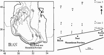
Mazandaran Province is located in the middle of the southern beach of the Caspian Sea along the Iranian coast. The gradient and structure of the seabed are uniform in this area. There is almost no tidal current. The surface salinity to 30 m depth varies negligibly (Hadjizadeh Zaker et al., Reference Hadjizadeh Zaker, Ghafari and Jamshidi2007). No major rivers exist in the vicinity of the sampling sites but the most important phenomenon in these areas is strong rip currents so that a lot of swimmers are killed by it every year. Sampling was conducted on the Noor coast (between Royan and Rostamrood) within 51°59′35″ to 52°02′31″E and 36°35′25″ to 36°36′29″N (Figure 1).
Map of sampling area.

Data collection
Seasonal samplings were carried out along three different depths (5, 15 and 30 m) in four transects (12 stations in total) during 2005 (Figure 1). Three replicate samples were collected at each station using a 250 cm2 Van Veen grab (Mistri et al., Reference Mistri, Fano, Ghion and Rossi2002). The contents of each grab were gently sieved in the field using 0.5 mm mesh and retained material fixed in 4% buffered formalin and stained with rose Bengal (Abrantes et al., Reference Abrantes, Pinto and Moreira1999). In the laboratory, macrofauna were sorted under stereomicroscope, identified and counted.
Another three separated replicate sediment samples were taken on each station for measured percentage of total organic matter (TOM) and sediment grain size by 250 cm2 Van Veen grab. Sediment from the surface (≈4 cm) was sub-sampled and stored in a cleaned plastic container (MacLeod et al., Reference MacLeod, Crawford and Moltschaniwskyj2004). Total organic matter was determined by weight loss on ignition (4 hours at 550°C) after drying (24 hours at 70°C) to constant weight (Abrantes et al., Reference Abrantes, Pinto and Moreira1999). To determine sediment particle size nearly 150 g of each grab sample was submitted to standard dry-sieve through a series of mesh sizes (from 63 µ to 2 mm) and mechanically shaken for 10 minutes. The sediments retained on each sieve were weighed and the percentage of each grain size category was determined (Diaz-Castaneda & Harris, Reference Diaz-Castaneda and Harris2004).
The macrobenthic community structure was described by univariate analysis based on the following parameters: density, species number (S), diversity (as Shannon–Wiener's, H′), richness (as Margalef's, D), and evenness (as Pielou's, J). The mentioned parameter values per square metre were calculated at all stations. Prior to analysis, data were tested for normality (using Shapiro–Wilk) and homogeneity of variance (using Levene's test). Significance of all tests was accepted at P < 0.05. Whenever data were normal and homogeneous, two-way analysis of variance (ANOVA) (station × season) was used to test for temporal and spatial differences in the physical parameters (TOM, sand and silt–clay percentage) and biological parameters (density, diversity, richness and evenness). Tukey's test was used to assess significant differences between stations and seasons. The significance level adopted was P < 0.05. The correlation of ecological indices with percentage TOM, sand and silt–clay, were determined using the Pearson's rank-correlation coefficient. The frequency of occurrence (F%) of the species was calculated according to Arasaki et al. (Reference Arasaki, Muniz and Pires2004). Based on this matter, we classified the species as constant (F > 50%), common (10% ≤ F ≤ 50%) and rare (F < 10%).
For understanding which sediment characteristics had the greatest influence on faunal composition and structure, principal component analysis (PCA) was applied to a correlation matrix of three sediment characteristics. Percentage of TOM, sand and silt–clay are plotted in two-dimensional space. Before this analysis, data of sediment characteristics had been standardized by: y = (x–xm)/sx, where y = standardized variable, x = not standardized variable, xm = mean value of x and sx = standard division of x. Data on the density of species were employing multivariate statistical methods of classification and ordination. The data were transformed by Log (x + 1). Similarity was calculated using the Bray–Curtis coefficient. Non-metric multidimensional scaling (nMDS) was used to analyse changes of macrofauna communities over the experimental period. Species with one individual and oligochaeta were eliminated for these analyses (Diaz-Castaneda & Harris, Reference Diaz-Castaneda and Harris2004). All the data from the four stations at each depth (three replicates, totaling 12 samples from each depth) were considered as a line (L1= 5 m, L2= 15 m and L3= 30 m) and the lines from different seasons were compared (Figure 1).
RESULTS
The benthic environment
The percentage of TOM, sand and silt–clay are shown in Table 1. Two-way ANOVA revealed significant differences among stations and seasons and also their interaction (Table 2). Maximum TOM was obtained in summer while minimum was observed in winter. Maximum and minimum percentages of sand were obtained in spring and winter, respectively. Maximum percentage of silt–clay was obtained in winter while the lowest amount was observed in spring.
Mean sediment variable measured during this study.

TOM, total organic matter.
Results of two-way ANOVA (station, season and interaction) on all of the analyses.

TOM, total organic matter.
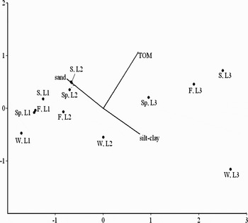
The result of the PCA is shown in Figure 2. Two first axes explained 98.28% of the total variance which indicated the study area could be divided in two regions based on the sediment characteristics. Group PCA I corresponded to the areas with shallow and intermediate depth area (5 and 15 m) and high percentage of sand and PCA II to deeper area (30 m) with high percentage of TOM and silt–clay.
Principal component analysis spatial presentation of stations based on sediment characteristics. W, winter; Sp, spring; S, summer; F, fall (autumn); TOM, total organic matter. L1= line 1, L2= line 2 and L3= line 3.

Community structure
Polychaeta numerically dominated the macrofauna during this study. The mean proportion of Polychaeta was 96.61% of all the individuals. The next abundant groups were: Bivalvia, 1.35%, Oligochaeta, 1.15% and Amphipoda, 0.87%.
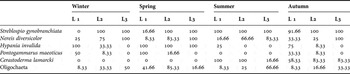
In the present study, three species of Polychaeta, Nereis diversicolor, Hypania invalida and Streblospio gynobranchiata, one species Bivalvia, Cerastoderma lamarcki, one species Amphipoda, Pontogammarus maeoticus and a few species of oligochaetes with a new alien to the Caspian Sea, Tubificoides fraseri (the other species were not identified) were observed. Presence and F% of them are shown in Table 3.
Frequency of occurrence during this study. L1 = line 1, L2 = line 2 and L3 = line 3.

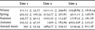
Two-way ANOVA revealed significant differences in densities among stations and seasons, also, significant interactions were observed so that the maximum of it was obtained in winter (Table 2). According to Tukey's test maximum and minimum densities were obtained in winter and summer, respectively. In general, density increased with depth. This increase was observed in all seasons (Table 4). It is necessary to mention that S. gynobranchiata was the dominant species during this study so that density of it was 84.95% of the total of obtained density.
Mean number of species recorded (per m2) in each season during this study.

Ecological indices
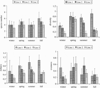
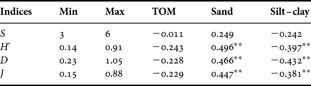
The ecological indices which include species number (S), diversity (H′), richness (D) and evenness (J) were calculated at each station (Figure 3). Two-way ANOVA revealed significant differences in diversity, richness and evenness among stations and seasons. Also, a significant interaction was observed among them except in evenness so that the maximum of these effects could be in winter (Table 2). The highest number of species (6 species) was obtained in line 1 in autumn and the lowest (3 species) was in line 3 in winter. The highest diversity (0.91) and richness (1.05) was in line 1 in autumn but the lowest (0.14 and 0.23, respectively) observed in winter. Maximum and minimum values of evenness were obtained in line 1 in summer (0.88) and line 3 in winter (0.15), respectively. In general, the values of the mentioned indices decreased with depths at all seasons. Also, Table 5 presents the minimum and maximum value of each index and its correlation with the measured factors of sediments.
Species number (S), diversity (H′), richness (D) and evenness (J) during this study.

Minimum (Min) and maximum (Max) values of the ecological indices measured. Pearson's rank-correlation coefficient value among the indices, total organic matter (TOM), sand and silt–clay.
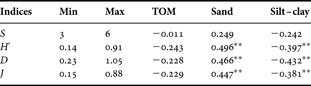
**, P < 0.01.
Multivariate analysis
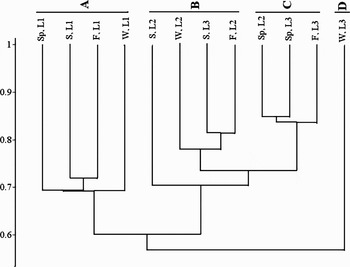
The Bray–Curtis analysis (Figure 4) separated four groups in relation to the sediment characteristics and depths: (A) comprised four lines at 5 m depth, density of this group was the lowest (211–455 ind/m2); (B) joined four lines at 15 m depth, density of this group was 1022–2211 ind/m2; (C) formed by three lines and density of this group was 3124–4211 ind/m2; and (D) comprised one line with the highest density value, its density was 10,548 ind/m2.
Similarity among lines using the Bray–Curtis coefficient. W, winter; Sp, spring; S, summer; F, fall (autumn). L1= line 1, L2= line 2 and L3= line 3.

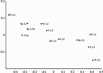
The nMDS ordination plot for the complete data is shown in Figure 5. The groups of lines separated by nMDS were very similar to those generated with the Bray–Curtis coefficient. Stress value was 0.018.
Non-metric multidimensional scaking plot of macrofauna communities. W, winter; Sp, spring; S, summer; F, fall (autumn). L1= line 1, L2= line 2 and L3= line 3.

DISCUSSION
In the present study, six species of macrofauna were identified. In the Baku Bay, Kasymov, (Reference Kasymov1989) found 9 species while Tait et al. (Reference Tait, Maxon, Parr, Newton and Hardin2004) obtained 62 and Parr et al. (Reference Parr, Tait, Maxon, Newton and Hardin2007) showed 71 species of macrofauna in the south of Baku, Azerbaijan. It should be mentioned that the present study was carried out at shallow water while Tait et al. (Reference Tait, Maxon, Parr, Newton and Hardin2004) and Parr et al. (Reference Parr, Tait, Maxon, Newton and Hardin2007) had sampled from shallow water to near 800 m depth. Although a lot of species of macrofauna were reported in the Caspian Sea (Birshtein et al., Reference Birshtein, Vinogradov, Kondakov, Astakhova and Romanova1968; Kasymov, Reference Kasymov1994), we did not find any communities of small forms such as Cumacea and Mysidacea in the study area. A similar result was obtained by Guseinov (Reference Guseinov2005) in Dagestan Region.
Although polychaetes have high species diversity among the macrofauna in marine ecosystems, fewer than ten species have been known in the Caspian Sea up to now (Birshtein et al., Reference Birshtein, Vinogradov, Kondakov, Astakhova and Romanova1968; Kasymov, Reference Kasymov1989, Reference Kasymov1994; Grigorovich et al., Reference Grigorovich, Therriault and MacIsaac2003; Tait et al., Reference Tait, Maxon, Parr, Newton and Hardin2004). In this study, only three species of them were found. Similar results were observed in the Gorgan Bay—south-west of the Caspian Sea—(Taheri et al., Reference Taheri, Seyfabadi and Yazdani Foshtomi2007; Bandany et al., Reference Bandany, Akrami, Taheri, Molla-Gholamali and Yelghi2008) and the south of Baku, Azerbaijan (Parr et al., Reference Parr, Tait, Maxon, Newton and Hardin2007). Also, our result showed the macrofauna was numerically dominated by Polychaeta as the same result had been obtained by Parr et al. (Reference Parr, Tait, Maxon, Newton and Hardin2007). On the other hand, Streblospio gynobranchiata was the dominant species during this study but according to Parr et al. (Reference Parr, Tait, Maxon, Newton and Hardin2007), Hypania invalida was the dominant species before arrival of S. gynobranchiata to the Caspian Sea. In other words, after arrival of S. gynobranchiata to this sea, the community structure of macrofauna has been changed. The same result was reported by Kotta et al. (Reference Kotta, Orav and Sandberg-Kilpi2001) after the invasion of Marenzelleria viridis in the north of the Baltic Sea. In the other seas, higher number of species has been reported, for example, in the Black Sea (Bulgarian region), 1192 species of macrofauna were reported (Golemansky, Reference Golemansky2007).
Salinity in brackish waters is one of the most important factors influencing distribution and dispersal of animals (Leppakoski & Olenin, Reference Leppakoski and Olenin2000). The south Caspian Sea has the most amount of salinity among all parts of this sea (about 13) and the lowest biodiversity in this part could be related to high salinity because a large number of the Caspian Sea fauna are endemic and adapted to live in waters with low salinity (Dumont, Reference Dumont2000). In this case, biodiversity in the southern parts is low and species with marine origin such as Streblospio gynobranchiata can live easily with high density in this part (Kasymov, Reference Kasymov1994).
During the last century, a lot of alien species arrived into the Caspian Sea (Grigorovich et al., Reference Grigorovich, Therriault and MacIsaac2003). Tubificoides fraseri had been originally reported in North America (Brinkhurst, Reference Brinkhurst1986) but there was not any report from the Caspian Sea before 2005 (Birshtein et al., Reference Birshtein, Vinogradov, Kondakov, Astakhova and Romanova1968; Kasymov, Reference Kasymov1989, Reference Kasymov1994; Grigorovich et al., Reference Grigorovich, Therriault and MacIsaac2003; Tait, et al., Reference Tait, Maxon, Parr, Newton and Hardin2004) so our study must be the first report of the existence of this species in the Caspian Sea. We guess it was transported into the Caspian Sea by ballast water via the Volga–Don canal.
Sediment grain size and TOM are two of the most important characteristics of macrobenthos dispersal (Nybakken, Reference Nybakken1993; Diaz-Castaneda & Harris, Reference Diaz-Castaneda and Harris2004). In this study, it was observed that the percentage of TOM and silt–clay increased with depths but sand percentage decreased (Table 1). Principal component analysis divided the study area in two different areas: (i) shallow and intermediate depth area (5 and 15 m) with high sand percentage; and (ii) deeper area (30 m) with the high percentage of TOM and silt–clay. Because Streblospio gynobranchiata was numerically dominant of macrofauna and with regard to this fact it is a deposit feeder (Cinar et al., Reference Cinar, Ergen, Dagli and Petersen2005) a higher density of macrobenthos found in deeper water may be related to TOM percentage increase (as a food) and sand percentage decrease.
Rip current is the most important phenomenon in the southern parts of the Caspian Sea. Although its velocity was not measured in the present study, maximum rip backwash velocities can reach to 1.6 m/s (McLachlan & Hesp, Reference McLachlan and Hesp1984). Rip current can disturb the sediment surface and transport fine parts to a deeper area (MacMahan et al., Reference MacMahan, Thornton, Stanton and Reniers2005) and also it can wash the meiofauna, macrofauna and zooplankton (macrofauna larvae) so that the distribution of them is related to rip current (McLachlan & Hesp, Reference McLachlan and Hesp1984). Also, it can wash TOM and indirectly effects the availability of organic matter used as food for macrofauna. Hence, it could be said that the effect of the rip current on sediment, TOM and washing macrofauna is another reason for increasing density with depths.
Seasonal density variation of the macrofauna is related to: (i) reproduction activity of macrofauna; and (ii) predator pressure (Mistri et al., Reference Mistri, Fano, Ghion and Rossi2002; Kevrekidis, Reference Kevrekidis2005). The highest density of macrofauna was observed in winter. This may be related to density of S. gynobranchiata that was maximal in this season (Taheri et al., Reference Taheri, Seyfabadi, Abtahi and Yazdani Foshtomi2009). The lowest density of macrofauna at all the sampled depths was recorded in summer; it may be related to: (i) the higher predation rate as reproduction season for many benthivore fish in the Caspian Sea starts from late winter to late spring; and (ii) higher metabolic rate, due to increase in temperature, associated with higher feeding intensity of predators.
Maximum species number (6), diversity (0.91) and richness (1.05) were very low. Similar results were obtained in the Gorgan Bay for Polychaeta (Taheri et al., Reference Taheri, Seyfabadi and Yazdani Foshtomi2007; Bandany et al., Reference Bandany, Akrami, Taheri, Molla-Gholamali and Yelghi2008). The value of these indices could be related to the small number of macofauna and existence of Streblospio gynobranchiata as the dominant species with very high density in each season.
The multivariate analyses indicated four macrobenthic groups related to sediment characteristics and depths. Stations with the low percentage of TOM and silt–clay and high percentage of sand were observed at group A with 5 m depth. This group had the lowest density. In group B, density of macrofauna increased rather than group A. Finally, in groups C and D, the highest densities were observed. The result of nMDS plot was observed to be very similar to similarity analysis. There is not any report about community structure of macrofauna at the south of the Caspian Sea. Hence we cannot compare the results of this study to other studies.
ACKNOWLEDGEMENTS
The authors are so thankful to Professor Christer Erséus and Mr Sebastian Kvist from the Department of Zoology, Gothenburg University, Sweden for identification of Tubificoides fraseri. We are also thankful to Mrs Shima Yazdani, A. Rashidi, A. Aliarab and R. Jamshidi for their assistance.