NOMENCLATURE
-
 ${A_r}$
-
atomic weight of ions
-
$B$
-
magnetic field strength
-
${\bf{b}}$
-
magnetic field vector
-
${{\bf{b}}^{\rm{p}}}$
-
induced-plasma magnetic field vector
-
$E$
-
electric field
-
${\bf{e}}$
-
inductive electric field vector
-
$I$
-
coil current
-
${\rm I}$
-
identity matrix
-
$N$
-
number of coil turns
-
${n_0}$
-
initial ion number density
-
${n_i}$
-
ion number density at nozzle inlet
-
$P$
-
pressure of an ideal gas
-
$R$
-
resistivity of plasma
-
$r$
-
coil radius
-
${S_{\rm{e}}}$
-
electron entropy
-
${T_e}$
-
electron temperature at nozzle inlet
-
${T_i}$
-
ion temperature at nozzle inlet
-
$t$
-
time
-
${\bf{u}}$
-
plasma velocity field vector
-
${u_{\rm{e}}}$
-
electron velocity
-
$v$
-
plasma inlet velocity
-
$z$
-
ion average charge number


Greek Symbols
-
${\gamma _e}$
-
electron adiabatic index
-
${\gamma _p}$
-
plasma adiabatic index
-
$\rho $
-
density
-
${\mu _0}$
-
vacuum permeability constant
-
$\psi $
-
numerical corrective term


1.0 Introduction
Pulsed inductive plasma (PIP) thrusters offer significant advantages when applied to interplanetary, cislunar, and manned space missions [Reference Polzin1]. These advantages include high specific impulse and relatively high thrust, utilisation of a wide variety of in-situ fuels, and scalability through pulse frequency. Such mission scenarios require these thrusters to possess reliability during long-term operation and adapt to a wide variety of thrust profiles. Their reliability and performance can be further enhanced through the application of non-mechanical thrust vectoring in the form of a magnetic nozzle. Compared with traditional means of beam steering such as mechanical gimbaling, magnetic nozzles have the advantages of reduction in weight, complexity, and throttle response time.
There have been several efforts to reveal magnetic nozzle physics through analytical modeling, numerical fluid/kinetic simulations, and experimental approaches. For instance, on the analytical modeling front, Arefiev and Breizman presented an ideal MHD analytic solution for plasma detachment in a magnetic nozzle [Reference Arefiev and Breizman2]. An axisymemetric steady-state numerical model for plasma flow in a magnetic nozzle [Reference Breizman, Tushentsov and Arefiev3] was later developed to compare against the analytical solution with good agreement. Other 2-D analytical models have been developed by Ahedo and Merino and their colleagues. These models include 2-D analytic axisymmetric model of supersonic acceleration in a divergent magnetic nozzle [Reference Ahedo and Merino4] and models of plasma expansion [Reference Ahedo and Merino5, Reference Merino, Cichocki and Ahedo6]. It was found through these models that the best way to increase divergence angle was to increase the initial ion Mach number.
On the numerical simulation front, existing approaches include 2-D fluid approaches to study the acceleration mechanisms [Reference Merino and Ahedo7], effects of induced magnetic field [Reference Merino and Ahedo8, Reference Merino and Ahedo9], detachment mechanisms [Reference Ahedo and Merino10, Reference Merino and Ahedo11], and effects of fully magnetized ions [Reference Merino and Ahedo12], as well as recent 3-D models [Reference Merino and Ahedo13] which have shown that increasing the current of the coils and maintaining constant solenoid current allowed for a less divergent plume. Hybrid particle-in-cell (PIC) and fluid approaches have also been used to study the nozzle regions and the external plasma environment [Reference Jiménez, Merino and Ahedo14]. Most recently, Hu et al. used an axisymmetric fullly kinetic PIC model to simulate magnetic nozzle expansion [Reference Hu, Huang, Cao and Sun15]. It was found that the fully kinetic model better approximated electron azimuthal current as compared to simplified fluid models. In addition to fluid and/or PIC approaches, a kinetic Boltzmann-Poisson model has also been recently introduced to study steady-state expansion of plasma in a paraxial convergent-divergent magnetic nozzle [Reference Zhou, Sanchez-Arriaga and Ahedo16]. Only electron-electron collisions were considered and including these collisions in the model resulted in a unique steady-state solution. In this model, the spatial profile in the convergent region was not affected but did increase density in the diverging nozzle as electrons became trapped. These electrons developed different temperatures and velocity distributions.
On the experimental front, a few studies have been carried out to study plasma detachment [Reference Deline, Bengtson, Breizman, Tushentsov, Jones, Chavers, Dobson and Schuettpelz17], plume potential profile [Reference Longmier, Bering, Carter, Cassady, Chancery, Chang Daz, Glover, Hershkowitz, Ilin, McCaskill, Olsen and Squire18], and controlling plasma flow direction [Reference Morita, Edamoto, Miura, Sunahara, Saito, Itadani, Kojima, Mori, Johzaki, Kajimura, Fujioka, Yogo, Nishimura, Nakashima and Yamamoto19]. Specifically to this study, a PIP source, namely the Missouri Plasmoid Experiment (MPX) [Reference Pahl20, Reference Meeks21], has been experimentally characterised. The MPX utilised field-reversed configuration (FRC) plasma generation to produce an initially magnetically self-contained plume [Reference Pahl, Meeks and Rovey22]. In MPX, the test article was initially filled with a neutral gas within a bias magnetic field. The neutral gas is pre-ionised and then the primary magnetic field is applied opposite to the bias field. This both fully ionises the plasma and creates a magnetically contained plasmoid. The benefits of this FRC plasma generation includes not needing an electrode and reduced plasma-wall interaction, which may lead to worn components and potential failure. Magnetic field and magnetic flux have been mapped by Pahl et al. in order to study plasma formation [Reference Pahl, Meeks and Rovey22, Reference Pahl and Rovey23]. Electron temperatures have been measured using a spectrometer to infer plasma formation time and pressure condition [Reference Meeks and Rovey24, Reference Meeks and Rovey25]. A few preliminary numerical studies using single particle models, iterative PIC, and circuit simulation models have then been performed to determine the optimal strength ratio between the bias field and pre-ionising/fully ionising field [Reference Meeks and Rovey26] and the primary loss mechanisms with FRC formation [Reference Meeks and Rovey27–Reference Pahl and Rovey29]. The numerical simulation campaign presented in this study was based on the operating parameters of MPX.
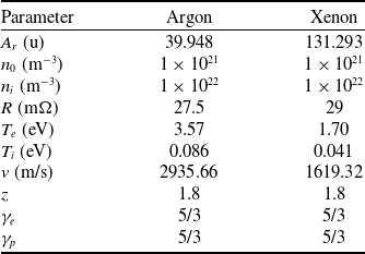
Initial plasma parameters

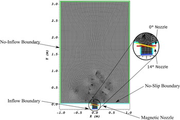
Mesh grid used for the simulations. The magnetic nozzle (shown in red) is positioned across the thruster exit at
 $y = 0$
m. The inflow boundary is positioned at the bottom edge of the grid at
 $y = -0.1173$
m. Axis values are in meters.

In this paper, we investigate a 2-D magnetic nozzle plume vectoring with the focus on plume angle in the immediate-downstream region of the nozzle with respect to coil current. Due to the high-density nature of the plume ejection of the PIP source studied in this paper [Reference Pahl and Rovey28], a fluid simulation approach has been chosen. Specifically, the fluid simulation software USim® [Reference Loverich and Hakim30], developed by Tech-X Corporation, was used. USim® is a fluid plasma modeling framework that simulates the dynamics of charged fluids or neutrals using structured or unstructured meshes. USim’s capabilities include solutions of compressible Euler equations for neutral gases, ideal MHD equations for ionised gases, Hall MHD, two-fluid plasma, and Navier-Stokes equations. It also supports the solution of multi-fluid multi-temperature equations for chemically reacting plasmas coupled with full Maxwell’s equations. The plasma flows chosen for this study were modeled after those experimentally determined from MPX [Reference Pahl and Rovey28].
The rest of this paper is organised as follows. Section 2 describes the theory of this plasma expansion model and setup of the simulations. Section 3 presents verification and validation of the simulation model and setup. Section 4 presents the results including phase-angle flow fields and long-time averaged flow fields when periodicity is obtained. Section 5 presents phase-angle and long-time averaged flow field values for different offset nozzle angles. Finally, a summary and conclusion is given in Section 6.
2.0 Theory and simulation setup
Magnetic nozzles work on the principle of opposing magnetic fields. The electrons, and to some extent ions, in a plasma create an induced magnetic field through their motion. This field directly opposes the field generated by the solenoidal coils in the nozzle. This propels the plasma through the nozzle. In addition, these opposing forces confine the plasma in the center of the nozzle. These effects were modeled using the USim® High Energy Density Plasma (HEDP) package.
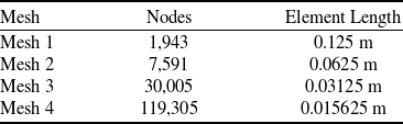
Meshes used in convergence study

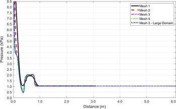
Argon pressure along
 $y$
-axis at
 $x = 0$
for the four mesh grids.

 ${T_e}$
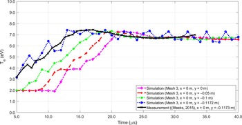
at four points in the nozzle region compared with experimental data for flow without an applied magnetic nozzle.

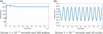
Pressure vs. time for argon.

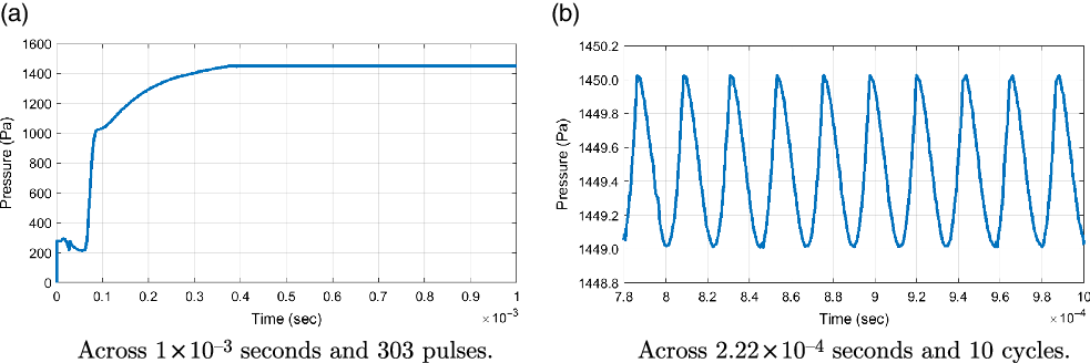
Pressure vs. time for xenon.

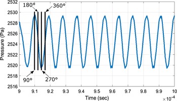
Definition of phase angles used for plotting.

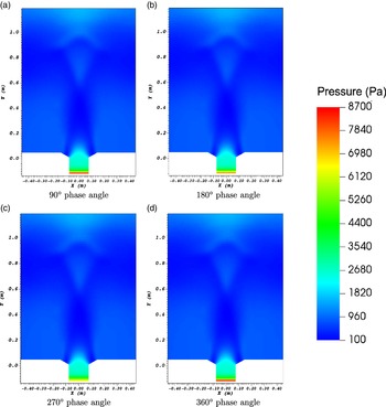
Pressure in Pa for argon at each phase angle starting at a time of
 $4.81111 \times {10^{ - 4}}$
seconds. Zoomed in near nozzle region.

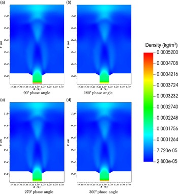
Density in kg/m
 $^3$
for argon at each phase angle starting at a time of
 $4.81111 \times {10^{ - 4}}$
seconds. Zoomed in near nozzle region.

 $y$
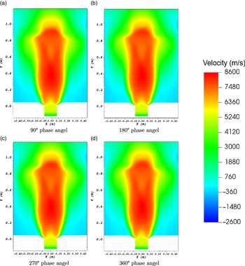
-velocity component in m/s for argon at each phase angle starting at a time of
 $4.81111 \times {10^{ - 4}}$
seconds. Zoomed in near nozzle region.

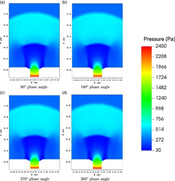
Pressure in Pa for xenon at each phase angle starting at a time of
 $4.81111 \times {10^{ - 4}}$
seconds. Zoomed in near nozzle region.

Density in kg/m
 $^3$
for xenon at each phase angle starting at a time of
 $4.81111 \times {10^{ - 4}}$
seconds. Zoomed in near nozzle region.

 $y$
-velocity component in m/s for xenon at each phase angle starting at a time of
 $4.81111 \times {10^{ - 4}}$
seconds. Zoomed in near nozzle region.

Long-time averaged domain pressure, density and velocity (in the
 $y$
-direction) for argon over 50 pulse cycles.

Long-time averaged domain pressure, density and velocity (in the
 $y$
-direction) for xenon over 50 pulse cycles.

First, the Biot-Savart law must be used to calculate the magnetic field strength, B, of a solenoidal coil using Eq. (1).
 \begin{equation} B = \frac{{{\mu _0}NI}}{{2r}} \end{equation}
where
 ${\mu _0}$
is the vacuum permeability constant, N is the number of turns in the coil, I is the coil current, and r is the coil radius. This field was then normalised by permeability of free-space. Next, the four ideal compressible magnetohydrodynamics (MHD) Eqs. (2)-(5) must be solved along with the entropy conservation Eq. (6).
 \begin{equation} {{\partial \rho } \over {\partial t}} + \nabla \cdot\left[ {\rho {\bf{u}}} \right] = 0 \end{equation}
 \begin{equation} {{\partial \rho {\bf{u}}} \over {\partial t}} + \nabla \cdot\left[ {\rho {\bf{u}}{{\bf{u}}^T} - {\bf{b}}{{\bf{b}}^T} + \textbf{I}\left( {P + {1 \over 2}|{\bf{b}}{|^2}} \right)} \right] = 0 \end{equation}
 \begin{equation} {{\partial E} \over {\partial t}} + \nabla \cdot\left[ {\left( {E + P} \right){\bf{u}} + {\bf{e}} \times {\bf{b}}} \right] = 0 \end{equation}
 \begin{equation}{{\partial {{\bf{b}}^{\rm{p}}}} \over {\partial t}} + \nabla \times {\bf{e}} + \nabla \psi = 0\end{equation}
 \begin{equation}{{\partial {S_{\rm{e}}}} \over {\partial t}} + \nabla \cdot\left[ {{S_{\rm{e}}}{u_{\rm{e}}}} \right] = 0\end{equation}
These five equations utilise the plasma density,
 $\rho $
, plasma velocity field,
 ${\bf{u}}$
, time, t, magnetic field,
 ${\bf{b}}$
, electric field, E, pressure of an ideal gas, P, inductive electric field,
 ${\bf{e}}$
, plasma magnetic field induced by the inductive electric field,
 ${{\bf{b}}^{\rm{p}}}$
, numerical corrective term,
 $\psi $
, electron entropy,
 ${S_{\rm{e}}}$
, and electron velocity,
 ${u_{\rm{e}}}$
.
For the simulations presented in this paper, USim® performed a second order upwind discretisation of a non-linear hyperbolic system for arrays of charge state, electric field, current, and resistivity. This was performed using a Riemann solver. The magnetic field and charge were updated. The current was calculated using the least squares gradient method on the magnetic field vector. The electric field was calculated using generalised Ohm’s law. This was done through integration using the Bulirsch-Stoer scheme. Finally, explicit time integration was performed using the Runge-Kutta method [31]. The plasmas under investigation are argon and xenon. These plasmas were chosen due to their prior use in experiments performed on MPX. These plasmas were defined in USim® using the following properties: atomic weight of ions,
 ${A_r}$
, plasma adiabatic index,
 ${\gamma _p}$
, electron adiabatic index,
 ${\gamma _e}$
, initial number density of ions,
 ${n_0}$
, temperature of ions at the nozzle inlet,
 ${T_i}$
, temperature of electrons at the nozzle inlet,
 ${T_e}$
, inlet velocity of the plasma, v, number density of ions at the nozzle inlet,
 ${n_i}$
, resistivity of plasma, R, average charge number of ions, z. The values used for the two plasmas are displayed in Table 1.
The plasma adiabatic index was kept the same for both species assuming mono-atomic plasma for a constant theta-pinch ratio of 0.29 resulting in a fully ionised gas [Reference Lee32]. The parameter values were chosen to replicate the conditions within MPX and were compared to literature values [Reference Pahl and Rovey23, Reference Meeks and Rovey27, Reference Jung, Surla, Gray, Andruczyk and Ruzic33]. The plasma was pulsed at the nozzle inlet in consecutive 3.3 microseconds cosine dependent cycles. The nozzle inlet diameter is 0.1550 m with a diverging outlet diameter of 0.2925 m. A coil-diameter-to-chamber-diameter ratio of 1.15 was chosen to replicate a nozzle fitted to the end of the MPX quartz chamber. The coil current was kept at 4,000 A through all runs with the exception of an extreme case at 14,000 A. This value was chosen due to its feasibility for future laboratory experimentation and for literature comparison [Reference Morita, Edamoto, Miura, Sunahara, Saito, Itadani, Kojima, Mori, Johzaki, Kajimura, Fujioka, Yogo, Nishimura, Nakashima and Yamamoto19]. It is noted here that the fluid approach using USim® is able to reveal the effects of induced magnetic fields.
Figure 1 shows the mesh grid and boundary conditions (BC) used for the simulations in this study. The
 $0^{\circ}$
nozzle was placed at the chamber exit at
 $y = - 0.001$
m. The inflow BC was applied at the bottom edge of the thruster at
 $y = - 0.004$
m. A no-slip BC was applied along the thruster walls and the edges perpendicular to the thruster. No-inflow BCs were applied on other domain edges. These no-slip and no-inflow boundary conditions were chosen following the suggestions in Marks et al., which showed that using a 2-D fluid plasma Dirichlet (no-slip) BC within a divergent nozzle and a zero-flux (no-inflow) BC on the domain exit matched well with experimental data [Reference Marks, Mikellides, Lopez Ortega and Jorns34].
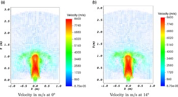
Argon velocity vectors at the time of
 $4.81111 \times {10^{ - 4}}$
seconds (90° phase angle) for 0° and 14° of nozzle offset (perpendicular to plasma flow).

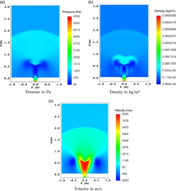
Long-time averaged domain pressure, density and velocity (in the
 $y$
-direction) for argon at a nozzle offset of 14°.

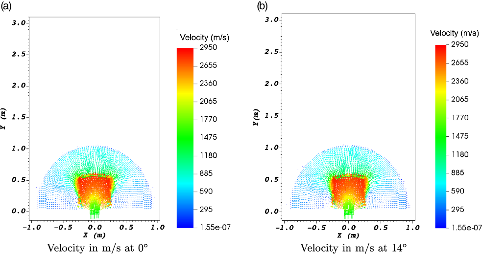
Xenon velocity vectors at a time of
 $4.81111 \times {10^{ - 4}}$
seconds (90° phase angle) for 0° and 14° of nozzle offset (perpendicular to plasma flow).

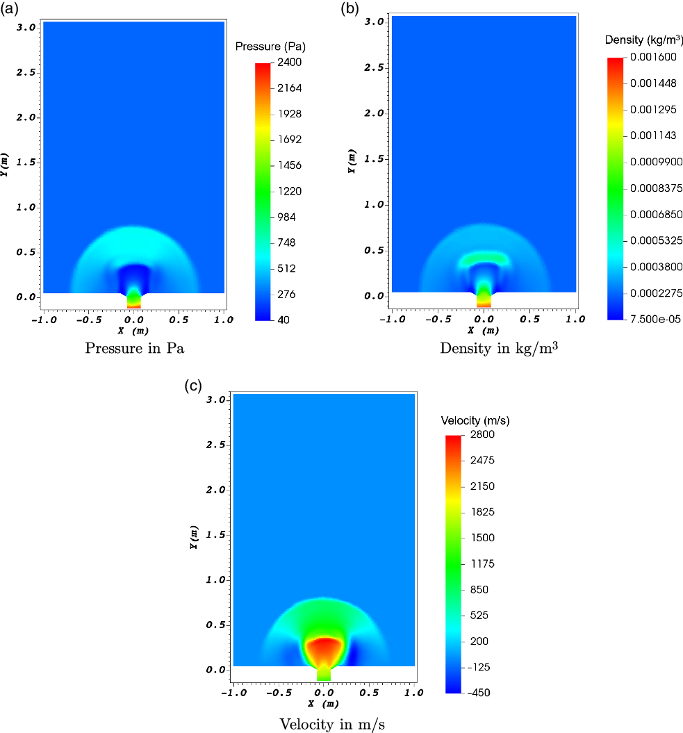
Long-time averaged domain pressure, density and velocity (in the
 $y$
-direction) for xenon at a nozzle offset of 14°.

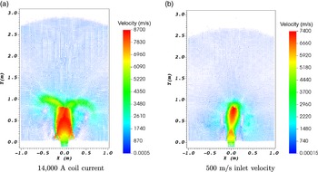
Velocity vectors in m/s for argon at 14° nozzle offset with extreme parameter values.

All the simulations were run until the physical elapsed time of
 $5 \times {10^{ - 4}}$
seconds from the quiet start, except the runs checking periodicity presented in Section 3.3, which ran until about
 $1 \times {10^{ - 3}}$
seconds. This simulation runtime corresponds to about 150 cycles of the plasma pulse (frequency of 303,030 Hz) and is long enough to ensure periodicity. A dynamic time step dependent on a Courant–Friedrichs–Lewy (CFL) condition of 0.4 was used to advance each step of the simulations. This time step was constrained to under
 $1 \times {10^{ - 8}}$
seconds. This choice of CFL number and time step size was based on the consideration of speed of solution and stability of the explicit integration scheme. All runs were performed on a Linux workstation equipped with two 8-core Xeon E5 CPUs with 64 GB of total memory. The runs were performed with an 8-core Message Passing Interface (MPI) configuration with an average computing time for each run of about 2 hours.
3.0 Model verification and validation
3.1 Mesh convergence
A mesh convergence study was performed for four grids. The number of nodes and element lengths for these four mesh grids are listed in Table 2. 1-D pressure-versus-distance profiles for argon were taken along the central vertical line of the domain and nozzle (
 $x = 0$
) at the simulation time of
 $1 \times {10^{ - 6}}$
seconds and plotted in Fig. 2. It was shown that the results converged at Mesh 3, which consists of 31,104 elements and 30,005 nodes with a 2-m by 3-m plume expansion domain. To ensure this domain is large enough with Mesh 3, we ran an additional case with an enlarged domain (doubled in both directions, 4-m by 6-m plume expansion region) with the same mesh resolution and plotted the 1-D pressure profile on Fig. 2 as well. Good agreement is shown between large-domain results and small-domain results. Therefore, Mesh 3 with 2-m by 3-m plume expansion domain was used for all runs presented in following sections.
3.2 Validation with experimental data
To validate our simulation model and setup using Mesh 3 and the 2-m by 3-m plume expansion domain, we ran the simulation model for a case of simple expansion into vacuum, without a magnetic nozzle (which was the configuration of MPX experiments [Reference Pahl20]) and compared results with experimentally measured data [Reference Meeks21]. Specifically, electron temperature
 ${T_e}$
was measured in the region downstream of the MPX chamber exit (which is the simulation domain in this study), and was used for direct comparison with our simulation results. Using the coordinates of the simulation domain, the experimental data point chosen for comparison was taken at the location of (x = 0 m, y = −0.1173 m), which is also the inlet of the simulation domain. From the simulation,
 ${T_e}$
history at four points just downstream of the inlet were also sampled over the simulation time period of 5 to 40 microseconds. These time history data of
 ${T_e}$
were plotted in Fig. 3. Good agreement between simulation and measurement was obtained for the location near the domain inlet (x = 0 m, y = −0.1172 m), where the simulation curve showed characteristic pulsed-cycle oscillations. The agreement was also achieved for the other three downstream locations after about 20 microseconds when the pulsed injection propagates downstream. This comparison validated our simulation model and setup.
3.3 Periodicity of simulation results
Pressure values were sampled at a rate of 20 per pulse cycle from the simulation start until periodicity was observed after
 $1 \times {10^{ - 3}}$
seconds. The mesh grid origin point was selected as the sample location since it is centered in the magnetic nozzle. These pressure-versus-time plots can be seen in Figs. 4 and 5 for argon and xenon, respectively. For both argon and xenon, the pressure built up and then leveled out. The xenon case took more time to build up pressure due to its larger atomic mass. Periodicity was achieved in approximately the same duration for both gas species.
4.0 Baseline results
We first present baseline results without applying a tilted/vectoring nozzle to check the phase angle values as well as long-time averaged flow field. Both argon and xenon were studied to check the pressure, density and velocity solutions.
4.1 Phase angle values
Once periodicity was reached, the phase angles of a cycle were defined as shown in Fig. 6 with 90° defined at the cycle peak value at the location of nozzle inlet (
 $x = 0,y = 0$
).
4.1.1 Argon
Pressure
Figure 7 shows argon pressure at different phase angles. At 90° the pressure at the inlet spikes to the highest value of 8,660 Pa. At 270° the lowest pressure of 6,020 Pa occurs at the inlet. Far-field values remain relatively constant. A lobed low-pressure region forms directly inline with the nozzle and expands outwards with the plume. These results are similar to those reported in the literature [Reference Merino and Ahedo7, Reference Jiménez, Merino and Ahedo14].
Density
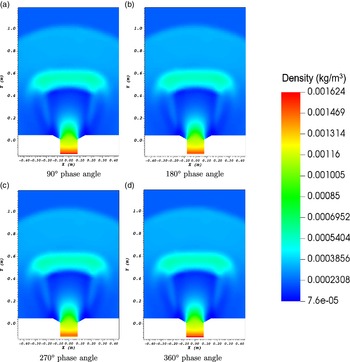
Figure 8 shows argon density at different phase angles. Density follows the same pattern as pressure with the highest value of
 $5.173 \times {10^{ - 4}}$
kg/m
 $^3$
occurring at 90° and the lowest value of
 $3.418 \times {10^{ - 4}}$
kg/m
 $^3$
occurring at 270°. A similar lobed low-density region forms but with stronger gradients bordering the medium density plume. Nuez et al. used a kinetic plume code combined with a two-fluid code to investigate the formation of a high-density region off-axis within the nozzle that follows the magnetic field lines [Reference Nuez, Merino and Ahedo35]. The results presented here show a high-density region within the plume but with a focusing effect towards the axis rather than following the field lines. Merino and Ahedo found that adherence of the plume to the field lines was determined to be a function of the ion magnetisation up to the fully magnetised ions limit [Reference Merino and Ahedo12].
Velocity
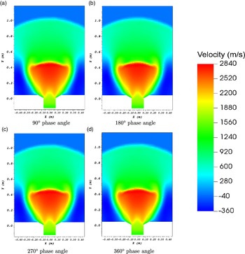
Figure 9 shows argon axial velocity at different phase angles. The inlet velocity changes only a few m/s over the phases and the far-field values remain relatively unchanged over this brief time period. The nozzle accelerative effect amounts to a velocity increase of 5,608 m/s over the value at the inlet. A high-velocity region forms directly along the plume axis and fans outwards. The nozzle field keeps the plume close to the central axis initially and then allows it to abruptly expand.
4.1.2 Xenon
Pressure
Figure 10 shows xenon pressure at different phase angles. At 90° the pressure values at the inlet spike to their highest value of 2,427 Pa. At 270° the lowest pressure of 2,310 Pa occurs at the inlet. Far-field values remain relatively constant. A less constricted and roughly trapezoidal low-pressure region forms directly inline with the nozzle and expands outwards with the plume. Both the argon and xenon cases show a narrowing of the plume at the nozzle exit.
Density
Figure 11 shows xenon density at different phase angles. Density follows the same pattern as pressure with the highest value of
 $1.624 \times {10^{ - 4}}$
kg/m3 occurring at 90° and the lowest value of
 $1.481 \times {10^{ - 4}}$
kg/m3 occurring at 270°. A similar trapezoidal low-density region forms but with stronger gradients bordering the medium-density plume with a prominent higher-density front, compared with the argon case.
Velocity
Figure 12 shows xenon velocity at different phase angles. The inlet velocity changes only a few m/s over the phases and the far-field values remain relatively unchanged over this brief time period. The nozzle accelerative effect amounts to a velocity increase of 1,232 m/s over the inlet value. A high velocity region forms directly along the plume axis and fans outwards. Unlike the way argon is constrained from expanding by the nozzle field, the xenon plume is able to expand directly after the outlet.
4.2 Long-time averaged flow field
The following long-time averaged flow fields were averaged over a series of approximately 50 pulse cycles from
 $3.4 \times {10^{ - 4}}$
to
 $4.7 \times {10^{ - 4}}$
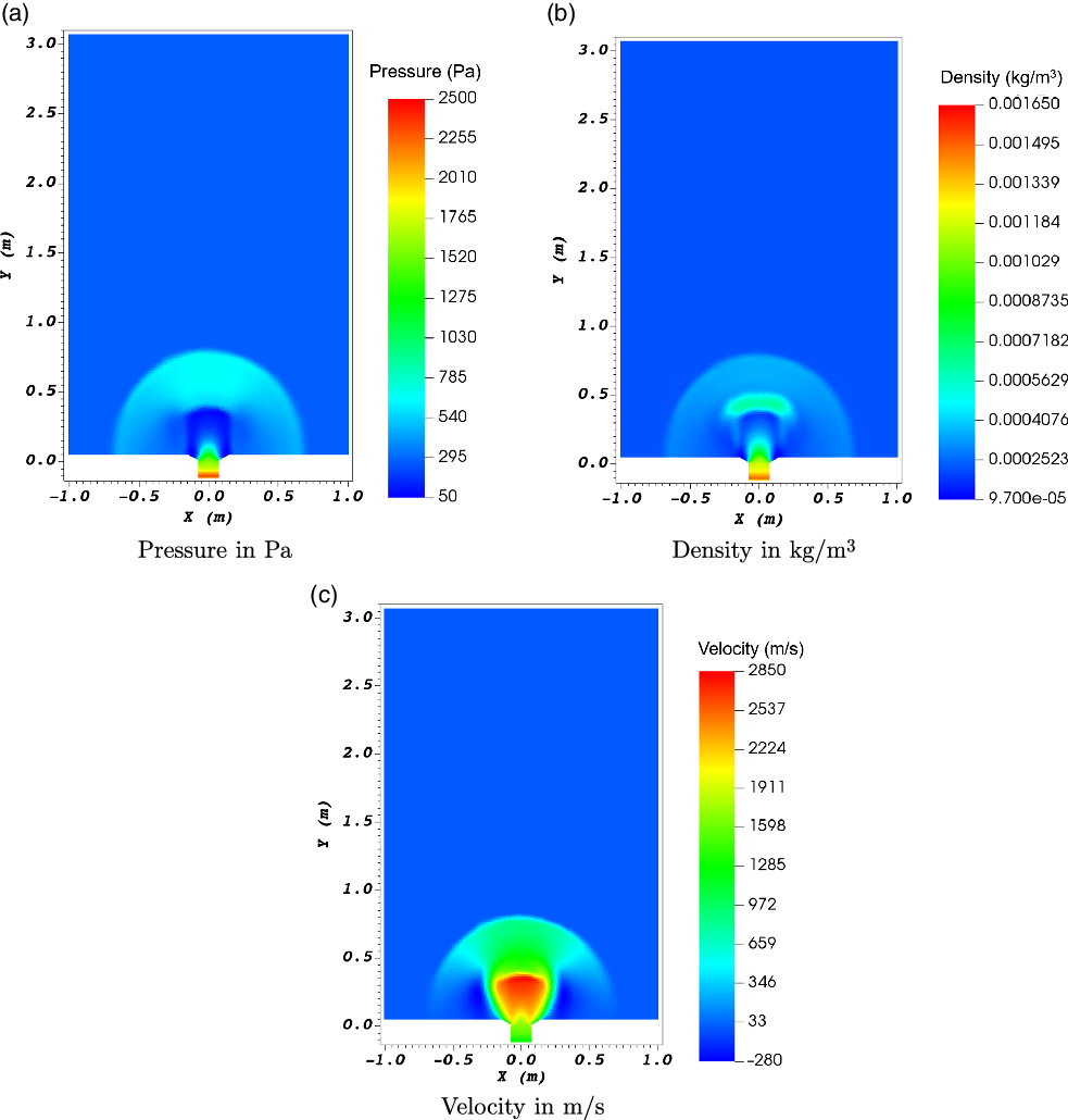
seconds with 20 data points per cycle. The long-time averaged flow fields for argon are shown in Fig. 13. The long-time averaged flow fields for xenon are shown in Fig. 14. These averages show similar plume profiles as the phase angle values. The long-time averaged fields show no significant difference from the phase angle plots. The same gradients can be seen across the flow fields indicating a gradual and steady increase in all three parameters.
After periodicity is achieved, there is very little difference in pulse cycle phase angle values except for regions near the inlet. These baseline results show steady far-field plume values and constant plume expansion. The nozzle performance can be inferred from the long-time averaged plots. With pulsed operation it is possible to emulate a steady state thruster plume with a focused ejection pattern. The distinct differences in argon and xenon plumes show that fuel selection is vital in determining thruster performance. Argon resulted in a more-focused plume with a greater gained velocity. Xenon showed a less-focused and immediately diverging plume that expanded approximately three times slower. The next step is to examine the effects on the plume resulting from offset magnetic nozzles.
5.0 Thrust vectoring using offset nozzles
For the simulations with offset (tilted) nozzles, the same inlet parameters were used except for the last two cases discussed in this section. The nozzle was offset at angles with respect to the domain x-axis as shown in Fig. 1. Eight runs were performed for both argon and xenon species from 0° to 14° of nozzle offset in 2° increments. Pressure, density and velocity long-time averaged flow fields were averaged over a series of approximately 30 pulses from
 $3.4 \times {10^{ - 4}}$
to
 $4.7 \times {10^{ - 4}}$
seconds for all the nozzle angles. The results show little distinction or plume vectoring among angles of 2° through 12° therefore these results were excluded from the analysis in this paper.
5.1 Argon
Figure 15 shows the velocity vectors for 14° offset angle at 90° phase angle along with the vector plots of 0° offset for comparison. Two arms can be seen curving from the plume back towards the nozzle inlet for both nozzle angles. It can be seen that the plume axis retains its accelerated direction while the plume edges are compelled to remain attached to the field lines. The 14° case shows a visible deflection in the plume arms and a bias in velocity magnitudes towards the right side of the plume. These vectors showed an average of 2.32° plume offset for argon. This value was found by averaging all plume vectors with magnitude larger than 6,500 m/s in order to find the vectoring angle of the primary plume region excluding far-field values. The argon velocity showed an increase of 5,644 m/s through the nozzle at 14°.
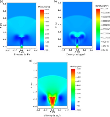
Figure 16 shows long-time averaged domain pressure, density and velocity (in the y-direction) for argon at the nozzle offset of 14°. Compared with the 0° case, maximum values of velocity and density remained relatively unchanged, while for pressure the maximum values decreased slightly (Fig. 13). A slight tilt of low pressure lobes in the plume region can be seen from the pressure plot. The pressure gradient pattern appears almost identical to the 0° case. The long-time averaged density plot shows the most distinct effect of nozzle angle, where a rightwards tilt in the low density lobes can be seen. The strong density gradient central to the plume shows separation, while the rest of the density gradients are similar to the 0° case. The y-direction velocity plot also shows a rightward tilt most prominently visible in the central plume region.
5.2 Xenon
Similar to the argon case, Fig. 17 shows the velocity vectors for xenon at 14° offset angle and 90° phase angle, in comparison with that of 0° offset. Both velocity vector plots look nearly identical. These vectors showed an average of 0.79° plume offset for xenon. This value was found by averaging all plume vectors with magnitude larger than 2,200 m/s in order to find the vectoring angle of the primary plume region excluding far field values. The xenon velocity showed an increase of 1,277 m/s through the nozzle at 14°.
Figure 18 shows long-time averaged domain pressure, density, and velocity (in the y-direction) for xenon at the nozzle offset of 14°. The offset profiles for xenon show no significant change in all three parameters. The pressure plot shows a flattening of the low-pressure region between the plume and nozzle. Asymmetry can be observed within the nozzle where higher values are seen as the plasma approaches the lower end of the coil. The density plot shows a slight rightward bias in the higher density front at the inner plume leading edge. The vectoring effect is better visualised through the y-direction velocity where the central plume region protrudes on the right side.
Overall, long-time averaged flow fields show argon has nearly three times the vectoring potential over xenon. The argon plume is more constrained near the nozzle exit by the magnetic field. The argon also shows a larger area of the plume separating and following the curvature of the field lines.
5.3 Argon using extreme parameter values
In order to explore the plume vectoring limits using extreme parameter values, two additional runs were carried out varying coil amperage or inlet plasma velocity for argon. The coil current was increased to 14,000 A in one case and the inlet velocity was decreased to 500 m/s in the other.
Figure 19 show velocity vectors of these two cases. These two runs resulted in increased plume offset angles of 4.35° when increasing amperage and 5.66° when decreasing velocity. The 14,000 A case shows a widened high velocity central plume region. The vectoring effect is more prominent, but so is the magnetic attachment. In this case, the requisite velocity for detachment was approximately 6,400 m/s determined by the highest values observed within the plume arms. While the coil amperage was increased by 10,000 A, the coil’s accelerative increase was minimal. The plume maximum velocity and vectoring angle increased by only 64 m/s and 2° respectively. The 500 m/s case shows greater promise in enhancing the thruster plume. Maximum velocity seen in the plume was 7,292 m/s, which is an increase of 6,792 m/s over the inlet value. The increase in vectoring angle of approximately 3.3° along with a velocity speedup of 14.6 times makes this a promising avenue for future studies. It is noted here that larger angles of plume vectoring have been reported in other studies. For instance, Merino and Ahedo demonstrated theoretically a 15° plume vectoring angle within a 3-D magnetic nozzle with three coils can be achieved [Reference Merino and Ahedo13], where the plasma density was about three orders of magnitude less than the values used in this paper. Another study by Morita et al. achieved 20° of plasma flow vectoring using two rectangular coils operated at 3 kA each with a pulsed laser plasma source [Reference Morita, Edamoto, Miura, Sunahara, Saito, Itadani, Kojima, Mori, Johzaki, Kajimura, Fujioka, Yogo, Nishimura, Nakashima and Yamamoto19], however the nozzle topology was quite different with no physical inlet wall to confine the flow.
6.0 Summary and conclusion
In summary, 2-D numerical simulations were carried out to quantify effects of magnetic nozzles for a representative PIP source. Simulations were verified and validated through a mesh convergence study as well as comparison with available experimental data. Periodicity of solutions was achieved when analysing phase-angle and long-time averaged flow field quantities. Both argon and xenon plasmas were investigated. Pressure values at different phase angles for a single pulse showed little variation in the plume and slight variation at the inlet. Long-time averaged flow fields showed little variation from the phase angle values due to the subtle effect the periodic inflow has after periodicity has been reached. The effects of a magnetic nozzle offset up to 14° show a maximum plume angle of 2.32° for argon and 0.79° for xenon. Improved angles were achieved through a significant yet unrealistic increase in coil amperage and decrease in inlet velocity. The effect of increased coil amperage on thruster performance showed a marginal velocity increase and approximately 2° additional vectoring at the cost of additional losses through greater magnetic attachment. The effect of decreased inlet velocity demonstrated an increase in plume vectoring angle and greater plume acceleration.
Based on the findings, we conclude that the application of a magnetic nozzle for steering the plume of a PIP source with the configuration and plume parameters presented here is not feasible for state-of-the-art in-space propulsion due to the large current required to achieve a useful offset angle. Further investigations are necessary to find a configuration that will allow for beneficial plume vectoring.
Acknowledgements
This work was partially funded by a NASA-Missouri Space Grant Consortium graduate fellowship.