1 Introduction
The wake of a flying animal provides the footprints that contain the physical information about the spatial–temporal characteristics of the fluid momentum associated with flapping flight. In principle, the aerodynamic forces acting on the animal could be inferred from either computed or measured velocity fields in the wake. The estimation of the aerodynamic forces from the wake velocity fields is advantageous since this method could circumvent some complex near-wall flow details related to the wing morphology and kinematics (Zhang Reference Zhang2017). In addition, the wake survey method is easier to implement in wind tunnel experiments and safer in laser flow diagnostics for flying animals. Therefore, considerable efforts have been made since the 1960s to estimate the aerodynamic forces and power (lift, drag/thrust and efficiency) from wake measurements (Pennycuick Reference Pennycuick1968; Rayner Reference Rayner1979a ,Reference Rayner b ; Spedding, Rosen & Hedenstrom Reference Spedding, Rosen and Hedenstrom2003; Dabiri Reference Dabiri2005; Li & Lu Reference Li and Lu2012; Lee et al. Reference Lee, Park, Jeong, Cho and Kim2013; Park et al. Reference Park, Park, Lee, Cho and Choi2016).
One of the favourable methods in estimating the lift is the application of the Kutta–Joukowski (KJ) theorem with the circulation computed in a Trefftz plane in the wake (Gutierrez et al. Reference Gutierrez, Quinn, Chin and Lentink2016). Here the Trefftz plane refers to a plane perpendicularly cutting through the wake (Gennaretti, Salvatore & Morino Reference Gennaretti, Salvatore and Morino1996). Since the KJ theorem is a cornerstone of classical aerodynamics for fixed-wing aircraft, it has been naturally adopted in studies of biological flapping flight due to its mathematical simplicity and physical clarity. However, it has been widely reported that the KJ theorem applied to experimental velocity data often underpredicts the time-averaged lift especially in slow-flying cases, and the estimated lift could be only 30–60 % of the weight of a bird or bat (Hubel et al. Reference Hubel, Hristov, Swartz and Breuer2009; Henningsson & Hedenstrom Reference Henningsson and Hedenstrom2011; Gutierrez et al. Reference Gutierrez, Quinn, Chin and Lentink2016). This puzzling underpredicted lift from the wake data in biological flapping flight is described by Spedding et al. (Reference Spedding, Rosen and Hedenstrom2003) as the wake momentum paradox.
The causes behind this paradox have been explored from different perspectives. The lower spatial resolutions of velocity measurements could lead to underestimation of the circulation, since some small vortex structures are not captured (Spedding et al. Reference Spedding, Rosen and Hedenstrom2003; Hubel et al. Reference Hubel, Hristov, Swartz and Breuer2009). Different experimental arrangements (Spedding & Hedenstrom Reference Spedding and Hedenstrom2009; Hubel et al. Reference Hubel, Riskin, Swartz and Breuer2010; Waldman & Breuer Reference Waldman and Breuer2012) have been proposed for improvements, such as manipulating the seeding particles, laser energy density and window sizes of particle image velocimetry (PIV), etc. Different data-processing methods to reduce the effects of measurement errors on the circulation estimation have also been proposed (Spedding et al. Reference Spedding, Rosen and Hedenstrom2003; Tian et al. Reference Tian, Iriarte-Diaz, Middleton, Galvao, Israeli, Roemer, Sullivan, Song, Swartz and Breuer2006; Hubel et al. Reference Hubel, Hristov, Swartz and Breuer2009). Estimation of the wake width is another critical issue in evaluating the lift, especially for the complex wake structures. The wingspan has been simply used by ignoring the wake contraction (Spedding et al. Reference Spedding, Rosen and Hedenstrom2003; Tian et al. Reference Tian, Iriarte-Diaz, Middleton, Galvao, Israeli, Roemer, Sullivan, Song, Swartz and Breuer2006; Hubel et al. Reference Hubel, Hristov, Swartz and Breuer2009). The spanwise distance between the peaks of the cross-sectional vorticity fields has been used as the wake width by Henningsson & Hedenstrom (Reference Henningsson and Hedenstrom2011), Muijres et al. (Reference Muijres, Bowlin, Johansson and Hedenstrom2012) and Gutierrez et al. (Reference Gutierrez, Quinn, Chin and Lentink2016). Furthermore, Muijres et al. (Reference Muijres, Johansson, Barfield, Wolf, Spedding and Hedenstrom2008) and Gutierrez et al. (Reference Gutierrez, Quinn, Chin and Lentink2016) have tried different ways to correct the incoming velocity by considering the local higher airspeed relative to the flapping wing due to the forward and vertical motions. However, although the careful set-ups of measurements and computations have improved the lift evaluated, the wake momentum paradox has not been fully resolved (Gutierrez et al. Reference Gutierrez, Quinn, Chin and Lentink2016).
Besides the above issues related to measurements, a more fundamental question is whether the KJ theorem itself is applicable to estimating the lift in highly unsteady wakes associated with biological flapping flight. The classical form of the KJ theorem was derived for a steady flow in the inviscid-flow framework. The KJ theorem has been recast in the viscous-flow framework where the Taylor–Sear condition with zero total vorticity flux has to be satisfied at the trailing edge. When the KJ theorem is applied to biological flapping flight, several assumptions are implicitly imposed. Firstly, it is assumed that the unsteady lift could be estimated as a quasi-steady vortex-related lift (simply called the KJ lift hereafter) at each moment. This quasi-steady assumption is not supported when the unsteady history of the lift is dominated by the inertial force associated with the fluid acceleration (Wang, He & Zhang Reference Wang, He and Zhang2013a ). Secondly, when the KJ theorem is applied to the Trefftz plane in the wake, it is assumed that the circulation calculated based on the streamwise vorticity on the Trefftz plane is equal to the bound-vortex circulation in the spirit of Kelvin’s total circulation conservation theorem. In general, this is not true for a complex viscous wake.
The objective of this work is to quantitatively investigate the applicability of the KJ theorem in estimating the lift for flapping flight. Three different flapping wing models are used to examine the limitations of the existing lift models based on the KJ theorem and evaluate the wake-sectional Kutta–Joukowski (WS-KJ) model proposed by the current work for flapping flight. The existing lift model based on the KJ theorem widely used in biological flapping flight and the way to evaluate the effective span length are discussed in § 2. The detailed results of applying the KJ theorem to three flapping wings are reported in §§ 3–5. Through numerical simulations of the flapping wings, the differences between the real lift and the KJ lift are discussed, indicating that the KJ theorem could not be directly used for estimating the unsteady lift. Then, it is found that the time-averaged KJ lift could be larger (overpredicted) or smaller (underpredicted) than the real one, depending sensitively on the locations of the selected Trefftz plane and the computation of the effective span length. Interestingly, when the WS-KJ model proposed by this work is used, the time-averaged KJ lift is consistent with the real lift, and the result is almost independent of the location of the selected Trefftz plane. The rationale behind this improvement is discussed. Further, the error source in estimating the time-dependent lift by using the KJ theorem is discussed. Finally, the conclusions are drawn in § 6.
2 Lift models for flapping wings
2.1 The widely used lift models
One of the widely used lift models for flapping wings is based on the KJ theorem and the quasi-steady assumption (Gutierrez et al. Reference Gutierrez, Quinn, Chin and Lentink2016), where the amplitude of the lift is given by
 $$\begin{eqnarray}\displaystyle L_{KJ}(t)=\unicode[STIX]{x1D70C}Ub\unicode[STIX]{x1D6E4}(t), & & \displaystyle\end{eqnarray}$$
where
 $\unicode[STIX]{x1D70C}$
is the fluid density,
 $U$
is the free-stream velocity encountered by the wing,
 $b$
is the effective span length, and
 $\unicode[STIX]{x1D6E4}(t)$
is the circulation around the airfoil. Here, the lift is defined as the force normal to the free stream, i.e. parallel to the
 $z$
-axis shown in figure 1. The corresponding lift coefficient is computed by
 $$\begin{eqnarray}\displaystyle Cl_{KJ}=\frac{L_{KJ}}{\unicode[STIX]{x1D70C}U^{2}S/2}=2\unicode[STIX]{x1D6E4}^{\ast }b^{\ast }G, & & \displaystyle\end{eqnarray}$$
where
 $S$
is the wing area,
 $\unicode[STIX]{x1D6E4}^{\ast }=\unicode[STIX]{x1D6E4}/(Uc)$
is the non-dimensional circulation,
 $c$
is the chord length,
 $b^{\ast }=b/c$
is the non-dimensional effective span length, and
 $G=c^{2}/S$
is a geometry parameter of the wing. For a rectangular wing with the effective span length of
 $b=S/c$
, equation (2.2) is simply
 $Cl_{KJ}=2\unicode[STIX]{x1D6E4}^{\ast }$
, which recovers the relation between the lift coefficient and the non-dimensional circulation for stationary airfoils. For a given wing with a fixed
 $G$
, equation (2.2) indicates that the lift coefficient is determined by the circulation around the airfoil and the effective span length.
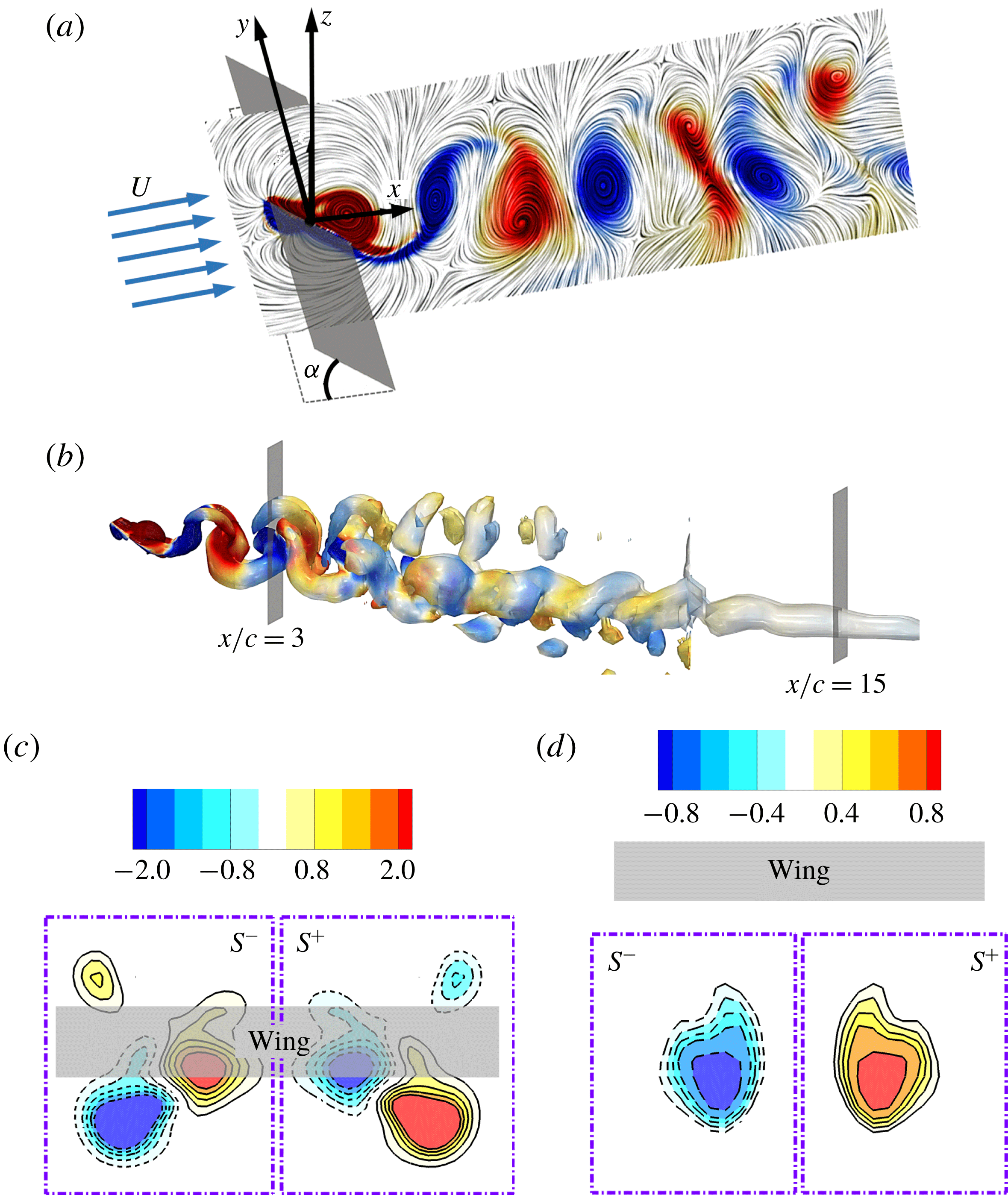
Schematics of the coordinate system and the integral domains in the Trefftz planes: (a) the flapping rectangular wing in a uniform upstream flow; (b) side view of the wake structures coloured by the spanwise vorticity from
 $-2$
(blue) to 2 (red); (c) streamwise vorticity fields in the Trefftz plane at
 $x/c=3.0$
; and (d) streamwise vorticity fields in the Trefftz plane at
 $x/c=15.0$
.

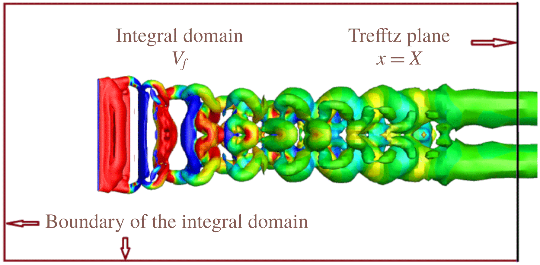
The coordinate system in figure 1 is used to describe the computation of the circulation in this work, where the
 $x$
-,
 $y$
- and
 $z$
-axes are parallel to the streamwise, spanwise and vertical directions with respect to the free stream, respectively. The circulation
 $\unicode[STIX]{x1D6E4}(t)$
is usually estimated from the streamwise vorticity in the wake (Hubel et al.
Reference Hubel, Hristov, Swartz and Breuer2009), i.e.
 $$\begin{eqnarray}\displaystyle \unicode[STIX]{x1D6E4}(t,X)=\int _{S^{+}(X)}\unicode[STIX]{x1D714}_{x}(t^{\prime })\,\text{d}S, & & \displaystyle\end{eqnarray}$$
where
 $S^{+}(X)$
denotes the right-hand side of the Trefftz plane at the streamwise location
 $x=X$
(see figure 1
c,d),
 $\unicode[STIX]{x1D714}_{x}$
is the streamwise component of the vorticity vector, and
 $t^{\prime }$
is the moment when the vorticity is measured in the Trefftz plane at
 $x=X$
. The translation between the lift-generating time
 $t$
and the delayed time
 $t^{\prime }$
is given by
 $$\begin{eqnarray}\displaystyle t=t^{\prime }-\frac{X-x_{t}}{U_{conv}}, & & \displaystyle\end{eqnarray}$$
where
 $x_{t}$
is the streamwise position of the trailing edge, and
 $U_{conv}$
is the convective velocity of the vortex structures in the wake. If the flow structures have a dominant velocity component, the dominant velocity is a reasonable approximation to the convective velocity. For simplicity, the incoming free-stream velocity is usually used as
 $U_{conv}$
in studies of biological flapping flight where the Strouhal number of the flapping flight ranges from 0.2 to 0.7 (Hedenstrom et al.
Reference Hedenstrom, Muijres, Busse, Johansson, Winter and Spedding2009; Hubel et al.
Reference Hubel, Hristov, Swartz and Breuer2009, Reference Hubel, Riskin, Swartz and Breuer2010; Muijres et al.
Reference Muijres, Spedding, Winter and Hedenstrom2011). The application of the free-stream velocity as
 $U_{conv}$
assumes that the vortex structures are frozen in the flow, which is tenable in the near and far wakes of a flying bat as reported by Hedenstrom et al. (Reference Hedenstrom, Muijres, Busse, Johansson, Winter and Spedding2009) and Hubel et al. (Reference Hubel, Hristov, Swartz and Breuer2009, Reference Hubel, Riskin, Swartz and Breuer2010). In other words, the time scales of the flow-structure propagations are faster than those of their changes. However, the application of the incoming free-stream velocity might not be valid for complex wake structures in slow forward flight since the strong interactions between adjacent vortices may via self- and mutual induction alter the mean flow (Hubel et al.
Reference Hubel, Riskin, Swartz and Breuer2010). The reduction of the distance between the Trefftz plane and the trailing edge is helpful to reduce the effects of the vortex-induced flow (Hubel et al.
Reference Hubel, Riskin, Swartz and Breuer2010). For the cases with complex wake structures, the convective velocity
 $U_{conv}$
can be globally determined through space–time correlations of velocity fluctuations (He, Jin & Yang Reference He, Jin and Yang2017) or locally determined by the phase velocities of energetic flow structures (del Alamo & Jimenez Reference del Alamo and Jimenez2009). In this work,
 $U_{conv}$
is taken as the incoming free-stream velocity, since it has been widely used in studies of biological flapping flight. Following the suggestion of Hubel et al. (Reference Hubel, Riskin, Swartz and Breuer2010), we use the Trefftz plane near the trailing edge (0.5 chord length downstream of the trailing edge) to reduce the effects of the vortex-induced flow when (2.4) is used to analyse the limitations of the widely used lift models. It is emphasized that the time-averaged (or ensemble-averaged) lift calculated in this study does not depend on the translation transformation equation (2.4).
The effective span length in (2.1) could be simply the wingspan (Spedding et al.
Reference Spedding, Rosen and Hedenstrom2003; Tian et al.
Reference Tian, Iriarte-Diaz, Middleton, Galvao, Israeli, Roemer, Sullivan, Song, Swartz and Breuer2006; Hubel et al.
Reference Hubel, Hristov, Swartz and Breuer2009), which is reasonable for a stationary wing with a large aspect ratio. For a stationary wing with a low aspect ratio, the wake width could be selected as the effective span length. For the unsteady flows in flapping flight, the wake width decreases as the vortex structures shedding from the flapping wing convect downstream, as discussed in § 3.4. Intuitively, for the varying wake width, a straightforward choice of
 $b$
is the spanwise distance between the peaks of the streamwise vorticity (DPV) in the Trefftz plane. The spanwise distance between the centres of the major vortex tubes could be approximately half of the wingspan, as shown in figure 1(d). However, as will be discussed in § 3, equation (2.1) based on the DPV fails to give a good prediction even for the time-averaged lift, and the estimated lift depends sensitively on the locations of the Trefftz planes. Moreover, since the wake structures of a flapping wing become complex, it is not easy to rationally determine the DPV when multiple peaks exist in the Trefftz plane. To circumvent this problem, we introduce the WS-KJ model.
2.2 Wake-sectional Kutta–Joukowski model
To take into account the distribution of complex vortex structures in the Trefftz plane, we propose the WS-KJ model as follows to compute the time-averaged lift:
 $$\begin{eqnarray}\displaystyle \langle L_{KJ}\rangle \approx \unicode[STIX]{x1D70C}U\langle b_{vor}(X)\rangle \langle \unicode[STIX]{x1D6E4}(t,X)\rangle . & & \displaystyle\end{eqnarray}$$
Here
 $\langle \unicode[STIX]{x1D6E4}(t,X)\rangle$
is the time-averaged circulation, and
 $\langle b_{vor}(X)\rangle$
is an effective span length defined by the vorticity-weighted width (VWW). The VWW is computed by
 $$\begin{eqnarray}\displaystyle \langle b_{vor}\rangle =2\frac{\left\langle \displaystyle \int _{S^{+}(X)}y\unicode[STIX]{x1D714}_{x}(t^{\prime })\,\text{d}S\right\rangle }{\left\langle \displaystyle \int _{S^{+}(X)}\unicode[STIX]{x1D714}_{x}(t^{\prime })\,\text{d}S\right\rangle }, & & \displaystyle\end{eqnarray}$$
where
 $\langle \bullet \rangle$
denotes the time-averaging operator, and
 $y$
is the spanwise position of the vorticity. When the vorticity-weighted width
 $\langle b_{vor}\rangle$
is substituted for
 $b$
in the time-averaged version of (2.1), it will be shown in the following sections that the predicted time-averaged KJ lift coefficient is in good agreement with the truth. In fact, equation (2.6) gives a time-averaged spanwise distance between the streamwise vorticity centroids in the right and left half sides of the Trefftz plane. The vorticity centroid was introduced by Saffman (Reference Saffman1970) for calculating the velocity of viscous vortex rings. It is somewhat surprising that such a simple scaling based on the vorticity-centroid distance,
 $\langle b_{vor}\rangle$
, leads to the correct prediction of the time-averaged lift by using the KJ theorem in the highly unsteady separated flow generated by a flapping wing. In fact, this dramatic improvement is not a fluke since there is a sound physical foundation for such scaling.
The lift acting on a body in an incompressible viscous flow is given by
 $$\begin{eqnarray}\displaystyle L=L_{vor}+L_{acc}+res, & & \displaystyle\end{eqnarray}$$
where the lift associated with the vortex (
 $L_{vor}$
), the lift associated with the fluid acceleration (
 $L_{acc}$
), and the residual term (
 $res$
) are expressed, respectively, as
 $$\begin{eqnarray}\displaystyle & \displaystyle L_{vor}=\unicode[STIX]{x1D70C}\boldsymbol{k}\boldsymbol{\cdot }\int _{V_{f}}(\boldsymbol{u}\times \unicode[STIX]{x1D74E})\,\text{d}V, & \displaystyle\end{eqnarray}$$
 $$\begin{eqnarray}\displaystyle & \displaystyle L_{acc}=-\unicode[STIX]{x1D70C}\boldsymbol{k}\boldsymbol{\cdot }\int _{V_{f}}\frac{\unicode[STIX]{x2202}\boldsymbol{u}}{\unicode[STIX]{x2202}t}\,\text{d}V-\unicode[STIX]{x1D70C}\boldsymbol{k}\boldsymbol{\cdot }\oint _{\unicode[STIX]{x2202}B}\frac{\boldsymbol{u}\boldsymbol{\cdot }\boldsymbol{u}}{2}\boldsymbol{n}\,\text{d}S, & \displaystyle\end{eqnarray}$$
 $$\begin{eqnarray}\displaystyle & \displaystyle res=-\boldsymbol{k}\boldsymbol{\cdot }\oint _{\unicode[STIX]{x1D6F4}}\left(p+\unicode[STIX]{x1D70C}\frac{\boldsymbol{u}\boldsymbol{\cdot }\boldsymbol{u}}{2}\right)\boldsymbol{n}\,\text{d}S+\boldsymbol{k}\boldsymbol{\cdot }\oint _{\unicode[STIX]{x1D6F4}}(\unicode[STIX]{x1D749}\boldsymbol{\cdot }\boldsymbol{n})\,\text{d}S. & \displaystyle\end{eqnarray}$$
In (2.8)–(2.10)
 $\boldsymbol{u}$
and
 $\unicode[STIX]{x1D74E}$
are the velocity and vorticity, respectively,
 $V_{f}$
is the control volume of the fluid,
 $\unicode[STIX]{x2202}B$
is the surface of the solid body,
 $\unicode[STIX]{x1D6F4}$
is the outer surface of the control volume enclosed by the solid body,
 $\boldsymbol{k}$
is the unit vector normal to the free-stream velocity, and
 $res$
is contributed by the total pressure and viscosity in the far field (Wang et al.
Reference Wang, Zhang, He and Liu2013b
). For an inviscid flow, Saffman (Reference Saffman1992) has given the same expression with
 $res=0$
. For the thin rigid wing considered in the present work, the contribution of the residual term to the lift is relatively small (as shown in § 3). The lift acting on the wing is dominated by the vortex lift and the local fluid acceleration around the wing.
Equation (2.8) can be written in the following form (see the details in appendix A):
 $$\begin{eqnarray}\displaystyle L_{vor}\approx \unicode[STIX]{x1D70C}U\int _{S(X)}y\unicode[STIX]{x1D714}_{x}\,\text{d}S. & & \displaystyle\end{eqnarray}$$
The time-averaged vortex lift in the far wake can be expressed as the time-averaged KJ lift, i.e.
 $\langle L_{vor}\rangle =\langle L_{KJ}\rangle$
as
 $X\rightarrow \infty$
, while the time-averaged contribution
 $\langle L_{acc}\rangle$
from the acceleration term is small as
 $X\rightarrow \infty$
or as the spatial integral and temporal average are taken (see more details in Wu, Ma & Zhou (Reference Wu, Ma and Zhou2006), Wang et al. (Reference Wang, Zhang, He and Liu2013b
) and Wu, Liu & Liu (Reference Wu, Liu and Liu2018)). Therefore, the asymptotic time-averaged KJ lift based on the flow in the Trefftz plane is
 $$\begin{eqnarray}\displaystyle \langle L_{KJ}\rangle \approx \unicode[STIX]{x1D70C}U\left\langle \int _{S(X)}y\unicode[STIX]{x1D714}_{x}(t^{\prime })\,\text{d}S\right\rangle =\unicode[STIX]{x1D70C}U\langle b_{vor}(X)\rangle \langle \unicode[STIX]{x1D6E4}(t,X)\rangle , & & \displaystyle\end{eqnarray}$$
where
 $S=S^{+}+S^{-}$
is the entire Trefftz plane consisting of the right and left sides denoted by
 $S^{+}$
and
 $S^{-}$
, respectively, as shown in figure 1. The first equality of (2.12) indicates that the time-averaged KJ lift is proportional to the integrated streamwise vorticity moment in the Trefftz plane. The second equality of (2.12) is in the classical form of the KJ theorem when the vorticity field is symmetrical in
 $S^{+}$
and
 $S^{-}$
. It is noted that, for the Trefftz plane at a finite distance, the contribution of the correlation term of the velocity fluctuations to the time-averaged vortex lift,
 $\langle L_{vor}\rangle$
(see the details in appendix A), is small and is neglected in this work, because both the spatial integral and temporal average suppress the contributions of the fluctuations to the time-averaged lift.
Since
 $\langle L_{KJ}\rangle$
should be independent of the location of
 $X$
, it is inferred that the quantity
 $\langle b_{vor}\rangle \langle \unicode[STIX]{x1D6E4}\rangle$
is conserved as the vortex structures travel downstream. For the steady flows over wings with a pair of parallel straight vortex lines or tubes, equation (2.6) results in a constant
 $\langle b_{vor}\rangle$
. In this limiting situation, the conservation of
 $\langle b_{vor}\rangle \langle \unicode[STIX]{x1D6E4}\rangle$
is equivalent to the conservation of
 $\langle \unicode[STIX]{x1D6E4}\rangle$
, and (2.12) reduces to the lift formula used in classical aerodynamics. However,
 $\langle \unicode[STIX]{x1D6E4}\rangle$
based on (2.3) is not conserved for a general distribution of the streamwise vorticity in Trefftz planes. In other words, the time-averaged total vorticity moment in the Trefftz plane is conserved in the wake instead of the conservation of the time-averaged circulation
 $\langle \unicode[STIX]{x1D6E4}\rangle$
which does not characterize the geometrical features of the vortex structures. The evolutionary effects of the vortex structures on both their strength and spanwise scale are explicitly incorporated in (2.12). This explains why the WS-KJ model improves the prediction for the time-averaged lift.
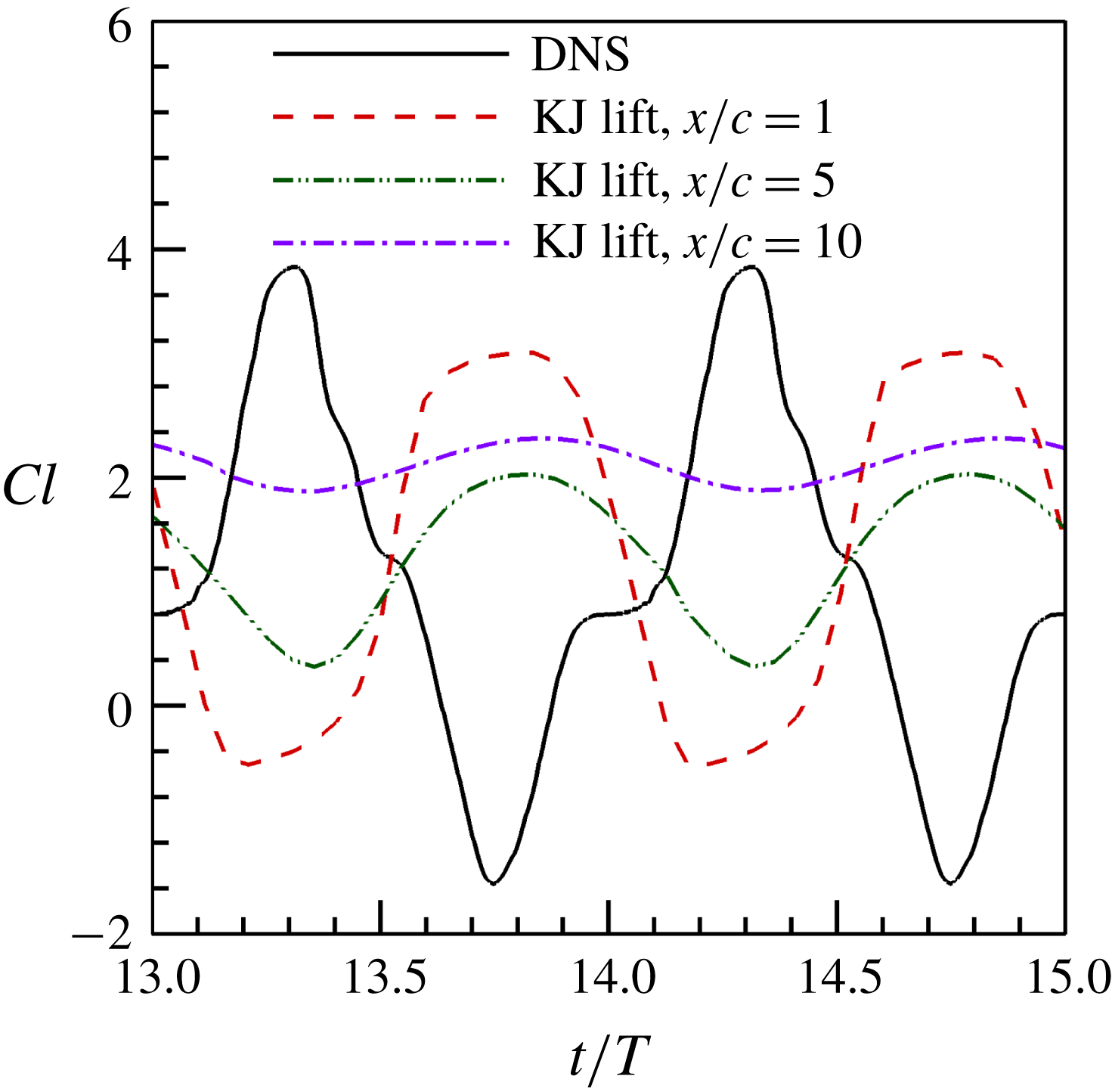
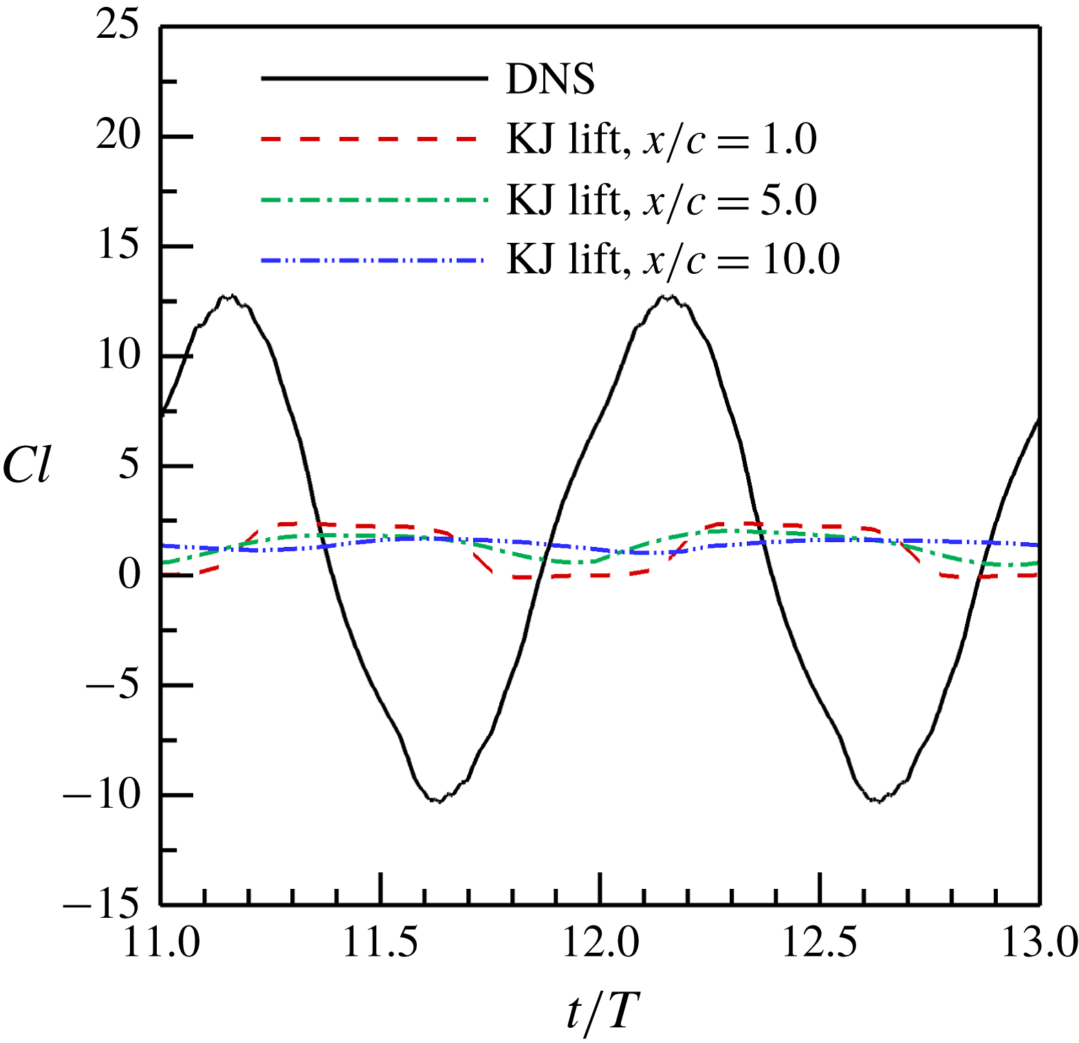
The time-dependent lift coefficients predicted by using the KJ theorem in different Trefftz planes for the flapping wing with a fixed wingspan. The wingspan is taken as the effective span length in computing the KJ lift.

The underlying assumption behind the proposed WS-KJ model is that the incoming free-stream velocity is sufficiently large in forward flight (hovering flight and very slow flight are excluded here). Further, this implies that the vorticities generated by flapping wings travel downstream at a significant convective velocity. The difficulties of the proposed model applied to the cases with low free-stream velocity (high Strouhal number) are discussed in appendix C. The proposed WS-KJ model provides a tool to compute the time-averaged lift based on the wake velocity data only on a Trefftz plane. There are several different methods to compute the aerodynamic forces based on the wake or near-wall flow fields (Wu Reference Wu1981; Chang Reference Chang1992; Noca, Shiels & Jeon Reference Noca, Shiels and Jeon1997; Dabiri Reference Dabiri2005; Wu et al. Reference Wu, Ma and Zhou2006). Different methods have different requirements on the time and space resolution of the velocity data. Detailed comparisons between several lift formulae are given by Wang et al. (Reference Wang, Zhang, He and Liu2015b ).
2.3 Unsteady effect
Based on the above analysis, the WS-KJ model with the vorticity-weighted width can give a good prediction of the time-averaged vortex lift, i.e.
 $\langle L_{KJ}\rangle \approx \langle L_{vor}\rangle$
, in which the effect of the fluid acceleration induced by a flapping wing is not incorporated. In the limiting case where a wing is in an inviscid flow, the lift associated with the fluid acceleration,
 $L_{acc}$
, can be interpreted as the added-mass lift,
 $L_{a}$
(Wang et al.
Reference Wang, Zhang, He and Liu2013b
). Therefore, equation (2.7) is approximately expressed as the superposition of the KJ lift and the added-mass lift, i.e.
 $L\approx L_{KJ}+L_{a}$
, which was derived by Liu et al. (Reference Liu, Wang, Zhang and He2015) in the unsteady viscous thin-airfoil theory.
The superposition
 $L\approx L_{KJ}+L_{a}$
provides a simple approximate method for estimating the unsteady lift of a flying animal from unsteady wake velocity data. Based on the classical unsteady thin-airfoil theory of Theodorsen (Reference Theodorsen1935), the added-mass lift coefficient of a heaving and pitching wing is modelled by
 $Cl_{a}=Ck^{\ast }$
, where
 $C$
is the scale factor associated with the added-mass coefficient,
 $k^{\ast }=\text{d}\unicode[STIX]{x1D6FC}/\text{d}t^{\ast }+\text{d}^{2}z_{c}^{\ast }/\text{d}t^{\ast 2}$
is the non-dimensional kinematical parameter, and
 $t^{\ast }$
and
 $z_{c}^{\ast }$
are the time and position of the wing normalized by the time scale
 $c/U$
and the wing chord
 $c$
, respectively. As will be shown in § 3, the added-mass lift has the same phase as the local fluid acceleration term. Indeed,
 $L\approx L_{KJ}+L_{a}$
can approximately recover the main phase and magnitude features of the real unsteady lift coefficient, when the KJ lift is estimated in the near wake.
3 Flapping wing with a fixed wingspan
3.1 Wing geometry and kinematics
Direct numerical simulations (DNS) of the flows over three flapping wing models with different wing geometry and kinematics are conducted (see appendix B for the details of the computational method and set-ups). We first investigate the application of the KJ theorem to a flapping rectangular wing. The flow structures (such as leading-edge vortex, trailing-edge vortex, tip vortices, etc.) and features of the aerodynamic forces in biological flapping flight can be generated by using a simplified flapping rectangular wing (Shyy et al.
Reference Shyy, Trizila, Kang and Aono2009; Li & Lu Reference Li and Lu2012; Guan & Yu Reference Guan and Yu2014; Yu et al.
Reference Yu, Amandolese, Fan and Liu2018). The rectangular wing used in this work is a zero-thickness plate with a fixed wingspan
 $b$
and a chord length
 $c$
. The aspect ratio of the wing is 4.0. The wing flaps in a uniform free-stream flow. Figure 1 shows the schematic of the model and coordinate system. The flapping kinematics of the model is described by
 $$\begin{eqnarray}\displaystyle & \displaystyle \unicode[STIX]{x1D6FC}(t)=\unicode[STIX]{x1D6FC}_{0}+\unicode[STIX]{x1D6FC}_{m}\cos (2\unicode[STIX]{x03C0}ft), & \displaystyle\end{eqnarray}$$
 $$\begin{eqnarray}\displaystyle & \displaystyle z_{c}(t)=z_{c0}+A\sin (2\unicode[STIX]{x03C0}ft), & \displaystyle\end{eqnarray}$$
where
 $\unicode[STIX]{x1D6FC}(t)$
and
 $\unicode[STIX]{x1D6FC}_{0}$
are the instantaneous and time-averaged angles of attack, respectively,
 $\unicode[STIX]{x1D6FC}_{m}$
is the pitching amplitude,
 $z_{c}(t)$
and
 $z_{c0}$
are the instantaneous and time-averaged vertical position of the wing centre, respectively,
 $A$
is the heaving amplitude, and
 $f$
is the pitching and heaving frequency. According to the set-ups of Wang et al. (Reference Wang, Zhang, He and Liu2014), the parameters used in the simulation are set at
 $\unicode[STIX]{x1D6FC}_{0}=10^{\circ }$
,
 $\unicode[STIX]{x1D6FC}_{m}=30^{\circ }$
,
 $z_{c0}=0$
,
 $A=0.25c$
and
 $f=0.6U/c$
, where
 $U$
is the free-stream velocity magnitude. The Strouhal number is
 $St=2fA/U=0.3$
, which is within the optimal Strouhal-number range for highly efficient swimming and flying animals (Taylor, Nudds & Thomas Reference Taylor, Nudds and Thomas2003). The Reynolds number is
 $Re=cU/\unicode[STIX]{x1D708}=300$
.
3.2 The Kutta–Joukowski lift
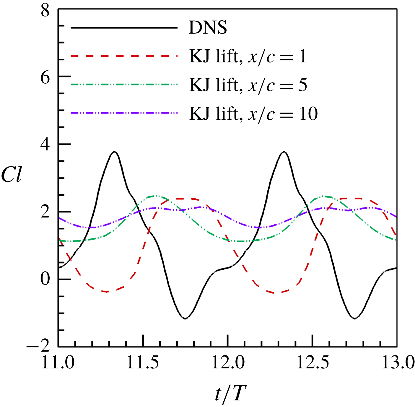
The KJ lift coefficients are calculated by using (2.2) with the circulation evaluated in different Trefftz planes. We first chose the wingspan as the effective span length, which is widely used in experimental investigations of biological flapping flight. The time-dependent lift coefficients estimated in three Trefftz planes are shown in figure 2 in comparison with the lift history obtained by integrating the surface pressure and skin-friction fields (hereinafter referred to as the DNS lift or DNS value). The KJ theorem with the circulations estimated in these Trefftz planes cannot correctly predict the time history of the unsteady lift. The estimated KJ lift is out of phase with respect to the DNS lift. The positive and negative peaks of the KJ lift are smaller (underpredicted), and the peak magnitudes decrease as the Trefftz plane moves downstream. It is clear that the KJ theorem cannot be used directly for estimating the unsteady lift from the wake data under the quasi-steady assumption. As will be pointed out in the following subsections, the differences in the phase and amplitude are caused by the fluid acceleration effect and the integral effect of the unsteady vortex evolution.
It has been found that the vortex lift mainly contributes the time-averaged lift of a flapping wing, while the fluid acceleration largely contributes the time variation of the lift (Wang et al.
Reference Wang, Zhang, He and Liu2013b
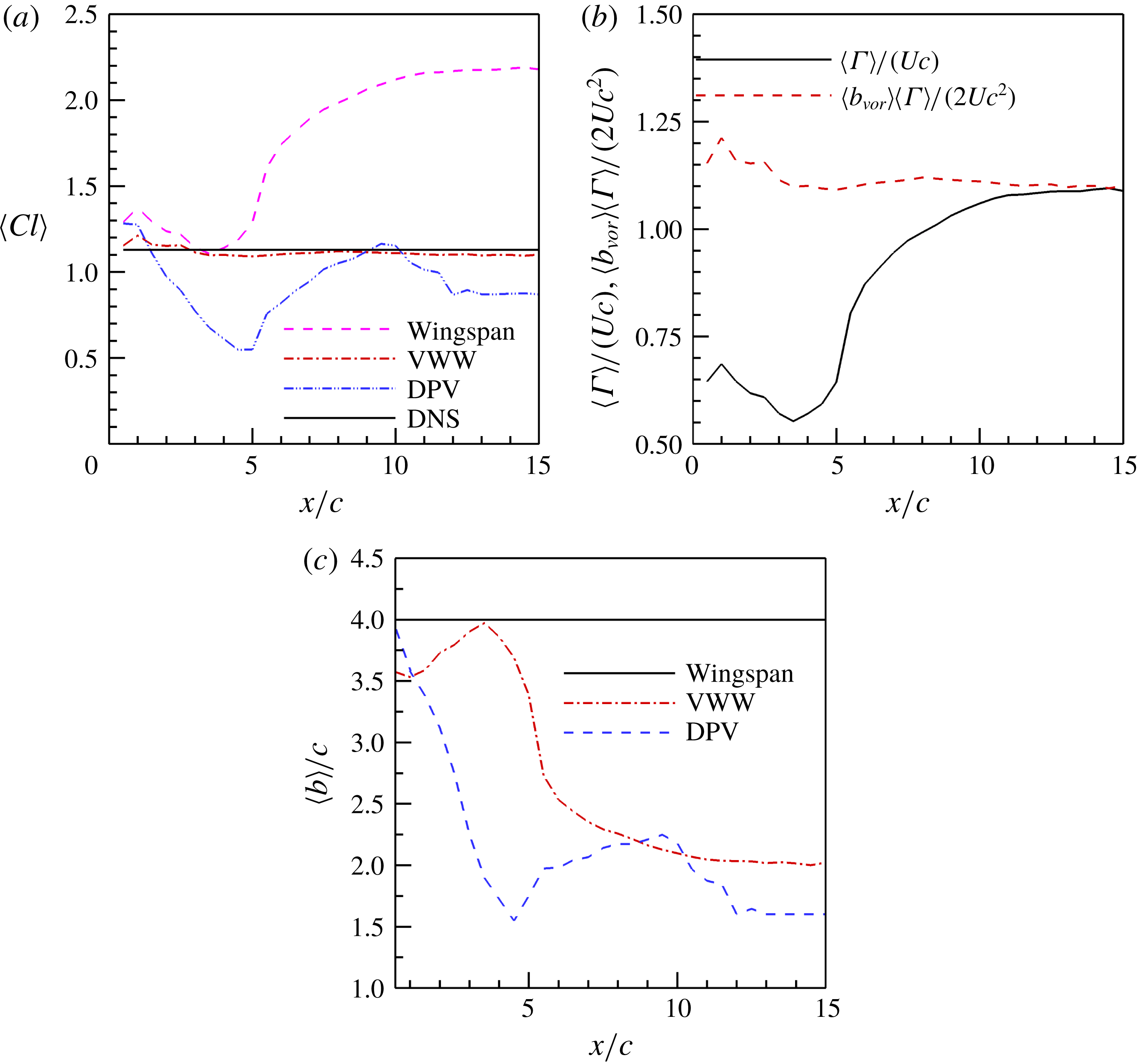
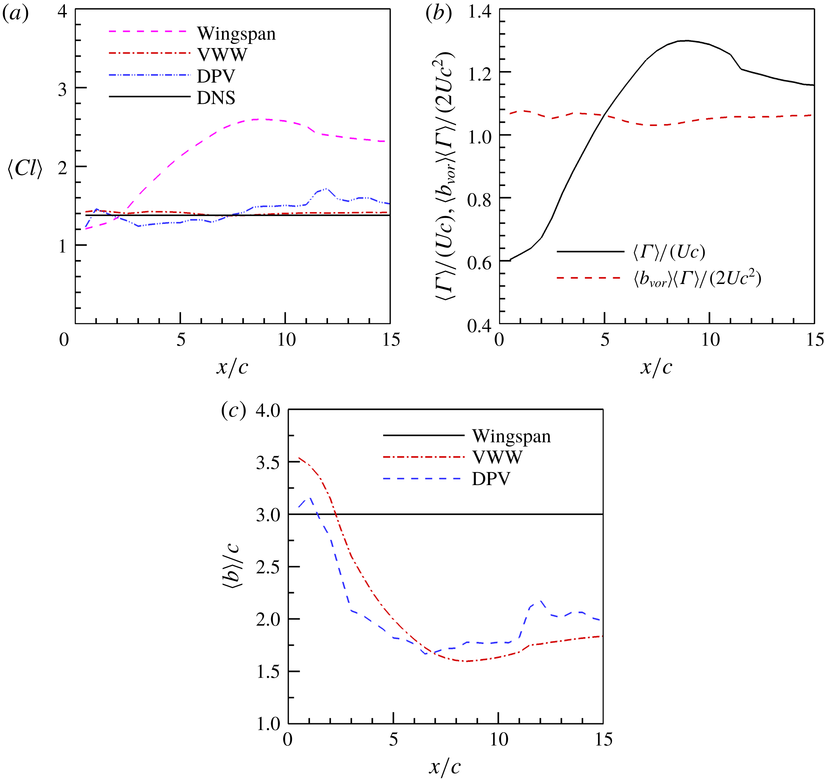
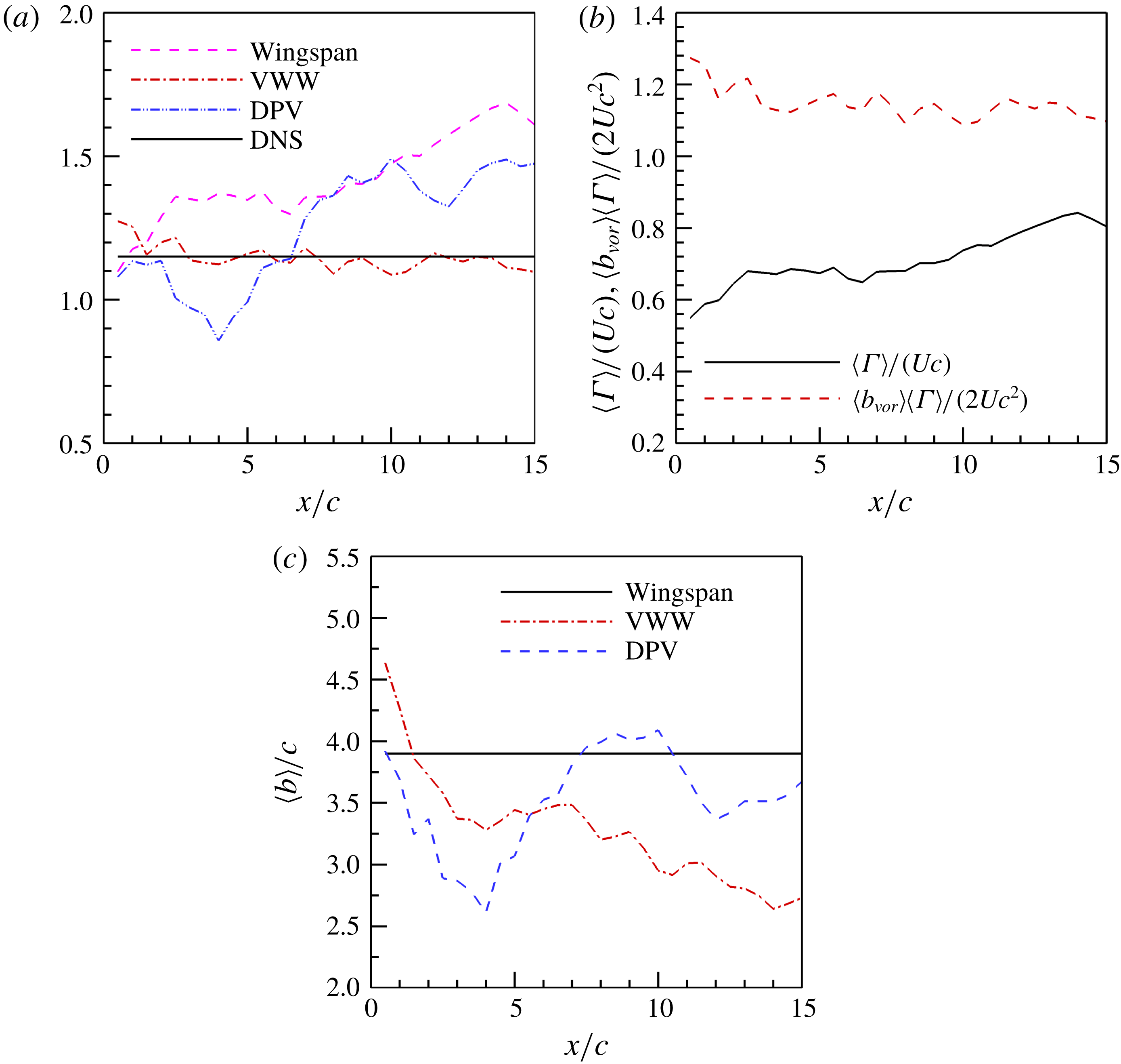
). An interesting question is whether the KJ lift as a special form of the vortex lift could give the time-averaging lift. The time-averaged KJ lift coefficient is evaluated as a function of the location of the Trefftz plane, as shown in figure 3(a). When the wingspan is selected for
 $b$
in (2.2), the time-averaged KJ lift coefficient
 $\langle Cl_{KJ}\rangle$
tends to be increasingly larger as the location of the Trefftz plane moves downstream. The predicted lift coefficient in the far wake (
 $x/c=15.0$
) is approximately twice as large as the real one. This overpredicted lift in this case is considered as another type of the wake momentum paradox. Then we chose DPV in the Trefftz plane for
 $b$
in (2.2). As shown in figure 3(a),
 $\langle Cl_{KJ}\rangle$
based on the DPV is underpredicted in most parts of the wake (
 $x/c>2.0$
), depending considerably on the location of the Trefftz plane. In contrast to the above cases, when the VWW,
 $\langle b_{vor}\rangle$
, is substituted for
 $b$
in (2.2),
 $\langle Cl_{KJ}\rangle$
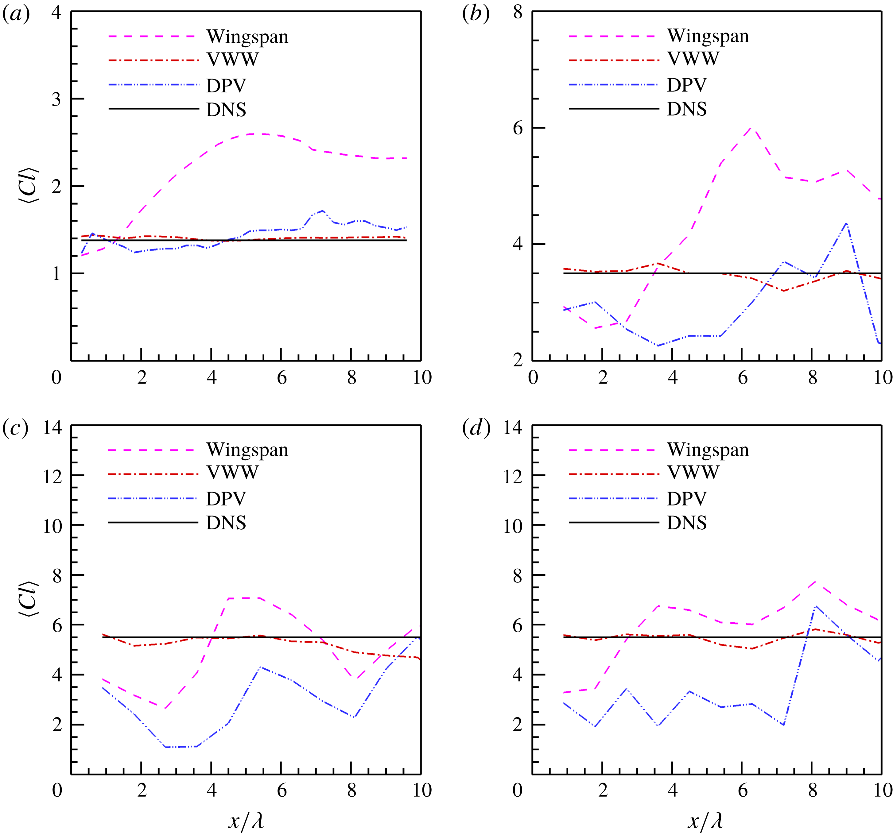
is in good agreement with the DNS lift (i.e. the WS-KJ model is used), and the relative error is within 3 % in the middle and far wake and within 6 % in the near wake, even though the grid resolution is relatively low in the far wake (as listed in table 1).
(a) Time-averaged lift coefficients predicted by using the KJ theorem with different effective span lengths; (b) time-averaged circulation and moment of the vorticity in different Trefftz planes; and (c) time-averaged wake widths computed by different methods for a flapping rectangular wing with a fixed wingspan.

For a stationary wing, the underlying assumption of using (2.2) for computing the lift coefficient is that the estimated circulation is independent of the location of the Trefftz plane. However, this is not true for a flapping wing. The circulation estimated based on (2.3) in the wake of a flapping wing depends on the location of the Trefftz plane, especially in the near-wake region. The time-averaged circulation as a function of the streamwise location of the Trefftz plane is shown in figure 3(b). The circulation slightly decreases in the near-wake region, increases steeply in the middle-wake region and approaches a constant in the far-wake region. The variation of the circulation reflects the evolution of the vortex structures in the wake, as discussed in detail in § 3.4. Figure 3(c) shows the variations of the time-averaged VWW and DPV in the wake. The time-averaged VWW defined in (2.6) gives a correct wake width to compensate the variation of the circulation in the wake. The product of the time-averaged VWW and circulation gives an estimated lift that is almost independent of the location of the Trefftz plane, as shown in figure 3(b). Although the time-averaged DPV varies with the location of the Trefftz plane, it cannot correctly represent the wake narrowing and does not vary inversely with the circulation (see the discussion in § 3.4).
3.3 Fluid acceleration and added-mass lift
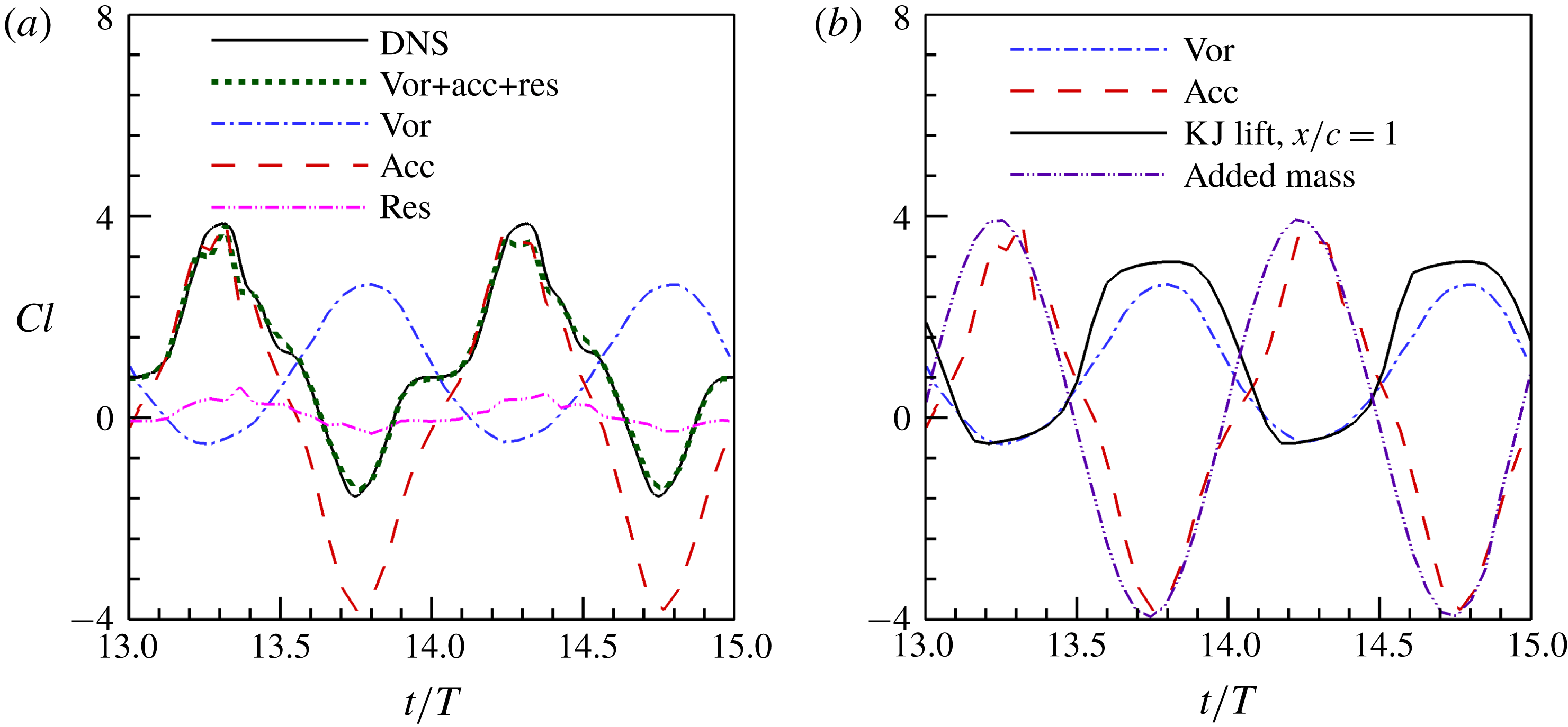
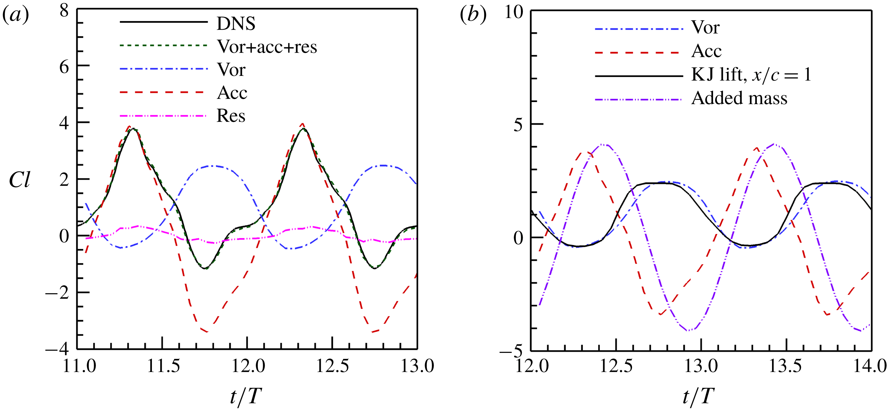
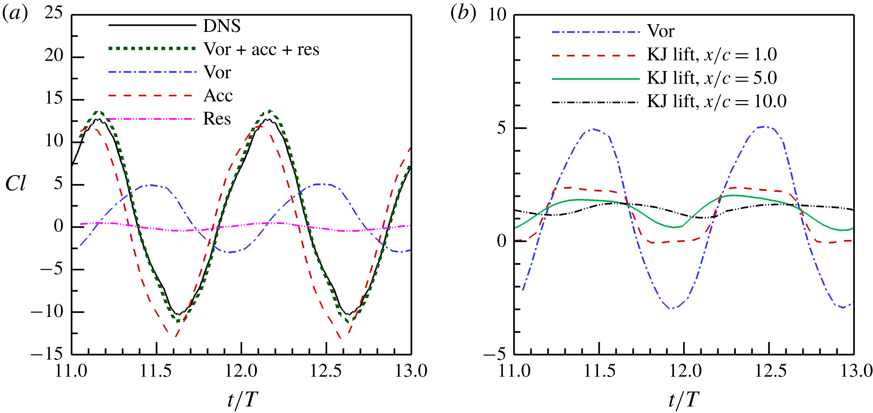
The KJ lift based on (2.1) is almost out of phase with the DNS lift, in addition to its decreasing magnitude as the Trefftz plane moves downstream, as shown in figure 2. We use the general lift formula, equation (2.7), to investigate the amplitude and phase of the unsteady lift. The lift is contributed by the vortex lift, local fluid acceleration and the residual term associated with the viscosity on the outer boundary of a control volume. For the thin rigid wing studied in this work, the contribution of the residual term to the lift is small when a sufficiently large rectangular control surface is selected to include all the vorticity structures around the wing and the accelerated fluid by the wing motions. The lift acting on the wing is dominated by the vortex force and the local fluid acceleration term (see figure 4
a), where the control volume is set to be
 $[-2.0c,x_{t}]\times [-6.0c,6.0c]\times [-12.0c,12.0c]$
, with
 $x_{t}$
the streamwise position of the trailing edge.
The decomposition of the lift based on (2.7) is shown in figure 4(a). It is found that the vortex lift is almost out of phase with the total lift and the maximum vortex lift is less than the maximum total lift. The lift associated with the local fluid acceleration term has approximately the same phase as the total lift. Nevertheless, the combination of the vortex lift and the local fluid acceleration term can recover more than 90 % of the total lift. As indicated before, the KJ lift is a reasonable approximation of the vortex lift for a thin wing. This is indicated in figure 4(b), where the KJ lift estimated in the Trefftz plane at
 $x/c=1.0$
is plotted along with the vortex lift. Note that the Trefftz plane at
 $x/c=1.0$
in the near wake is selected since the deformation and interaction of the wake vortex structures have a relatively small effect on the computation of the circulation (Hubel et al.
Reference Hubel, Riskin, Swartz and Breuer2010). Clearly, the quasi-steady assumption is not valid for the current flapping wing. The peaks of the KJ lift tend to decrease as a result of the integral effect of the deformation and interaction of the wake vortex structures in the wake.
(a) The decomposition of the lift coefficient by using the (2.7); and (b) the KJ lift, added-mass lift and their comparisons with the decomposed lift for the flapping rectangular wing with a fixed wingspan.

The local fluid acceleration term in (2.7) can be reduced to the added-mass lift in the viscous thin-airfoil theory (Liu et al.
Reference Liu, Wang, Zhang and He2015). We have tried to use a simple added-mass model given by Theodorsen (Reference Theodorsen1935) with the added-mass coefficient
 $C=-2.5$
(Korotkin Reference Korotkin2009) to approximate the local acceleration term. As shown in figure 4(b), the added-mass lift approximately recovers the local fluid acceleration term, and they have almost the same phase and amplitude. The superposition of the KJ lift and the added-mass lift,
 $L\approx L_{KJ}+L_{a}$
, is indeed able to recover approximately the main phase and magnitude features of the DNS unsteady lift coefficient. This result confirms that the KJ lift model with the quasi-steady assumption is not applicable to the current flapping wing. The added-mass effect should be considered to correctly estimate the instantaneous lift. It is emphasized that the KJ lift is evaluated in the near wake where the circulation is relatively less affected by the vortex deformation and interaction. However, when the KJ lift is evaluated in the middle and far wake, since the integrated (historic) effect of the vortex evolution is involved,
 $L\approx L_{KJ}+L_{a}$
is not able to recover the time-dependent lift. The integrated effect of vortex evolution is another reason that causes the differences between the KJ lift and the DNS lift. For the simple geometry and kinematics of this rectangular wing, the added-mass lift model is a good approximation of the local fluid acceleration term. For a wing with the complex planform and kinematics, modelling of the added-mass force is non-trivial, which is beyond the scope of this paper.
The KJ theorem was originally derived for a steady inviscid flow and then recast in the viscous-flow framework (Wu et al. Reference Wu, Liu and Liu2018). When the KJ theorem is applied to the flapping flight of birds or bats, it usually gives errors in the phase and magnitude due to the quasi-steady assumption (Sun Reference Sun2014; Gutierrez et al. Reference Gutierrez, Quinn, Chin and Lentink2016). To explicitly account for the unsteady effect, Sane & Dickinson (Reference Sane and Dickinson2002) proposed a revised quasi-steady model with several free parameters to be determined based on experimental and/or numerical data for a specific wing with known kinematics. The classical Theodorsen theory and Karman–Sear theory incorporate the unsteady added-mass force into the KJ model, which are useful in studies of biolocomotion without massive flow separation (Chopra Reference Chopra1976; Liu et al. Reference Liu, Wang, Zhang and He2015). Some semi-analytical models are able to account for the separated flow at the leading edge (Yu, Tong & Ma Reference Yu, Tong and Ma2003). More discussions on the lift models can be found in the reviews of Sane (Reference Sane2003) and Sun (Reference Sun2014). The mathematical and physical connections between different lift models are detailed by Wu et al. (Reference Wu, Liu and Liu2018). Compared to the existing models, the distinct feature of the present model is that an effective span length is introduced to account for the effects of the complex vorticity structures in the wake. The effective span length is defined as the time-averaged distance between the streamwise vorticity centroids. Therefore, the proposed model can correctly compute the time-averaged lift based on the vorticity field in a Trefftz plane.
3.4 Wake vortex structures
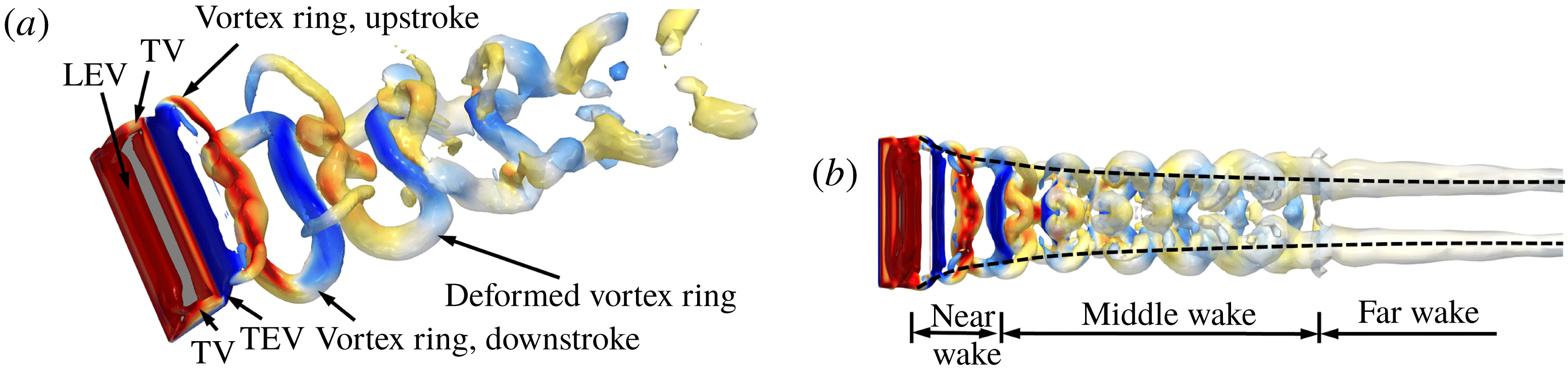
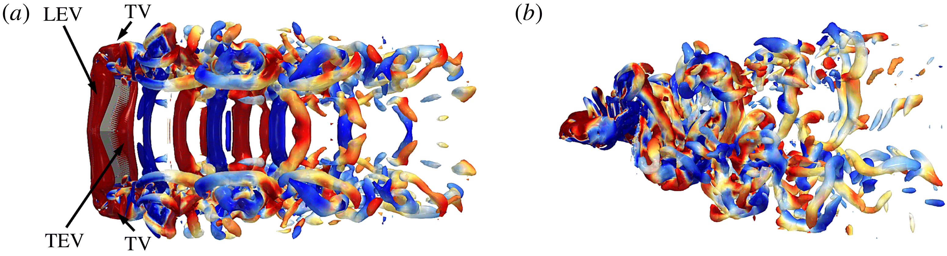
The selection of the effective span length in lift estimation directly depends on the development of the wake vortex structures. It is necessary to discuss the geometrical and dynamical features of these structures. The flapping rectangular wing generates the leading-edge vortex (LEV), tip vortices (TVs) and trailing-edge vortex (TEV) in downstrokes and upstrokes, as shown in figure 5(a). These vortices deform and interact with each other as they convect downstream. The details of the evolving vortex structures are described in our previous work (Wang et al.
Reference Wang, Zhang, He and Liu2014). Here, we focus on the main wake features which are closely related to the lift estimation. The wake can be approximately divided into three regions, as shown in figure 5(b). The near wake is from the trailing edge to
 $x/c\approx 3.0$
, where the LEV, TVs and TEV interact with each other to form vortex rings. The middle wake ranges from
 $x/c\approx 3.0$
to
 $x/c\approx 10.0$
, where the vortex rings deform considerably due to the mutual and self-induction and the wake is gradually separated into two branches (as shown in figures 1
b and 5
b). In particular, the wake narrows in the spanwise direction in the near- and middle-wake regions. The far wake starts from
 $x/c\approx 10.0$
, where the initial vortex rings generated in the downstroke and upstroke finally merge into two streamwise vortex tubes.
Wake structures of the flapping rectangular wing with a fixed wingspan: (a) perspective view with
 $Q=0.5$
, coloured by the normalized spanwise vorticity from
 $-10$
(blue) to 10 (red); and (b) top view with
 $Q=0.02$
, coloured by the normalized spanwise vorticity from
 $-1$
(blue) to 1 (red).

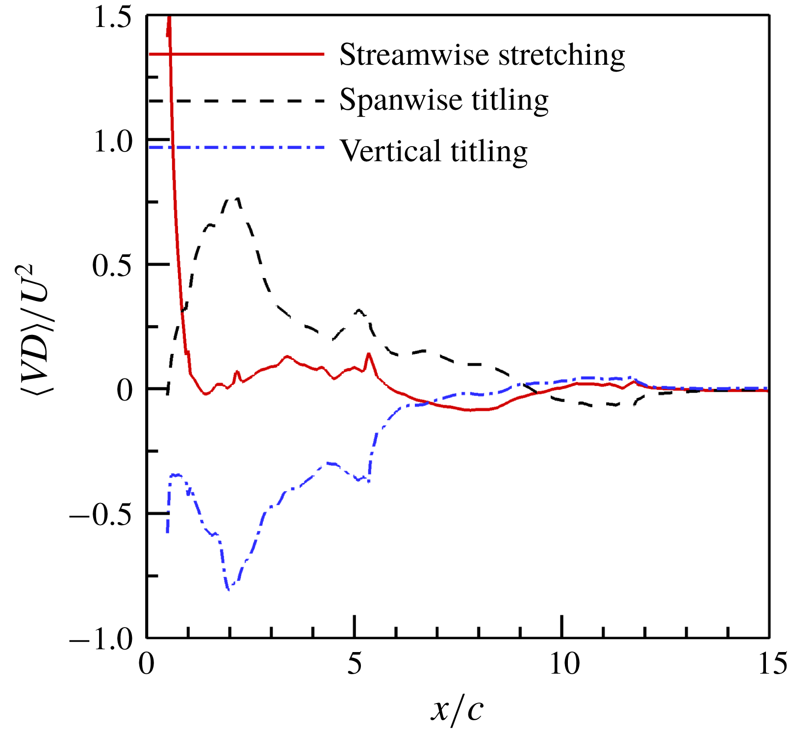
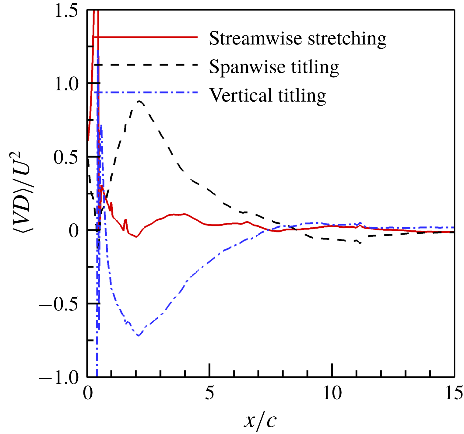
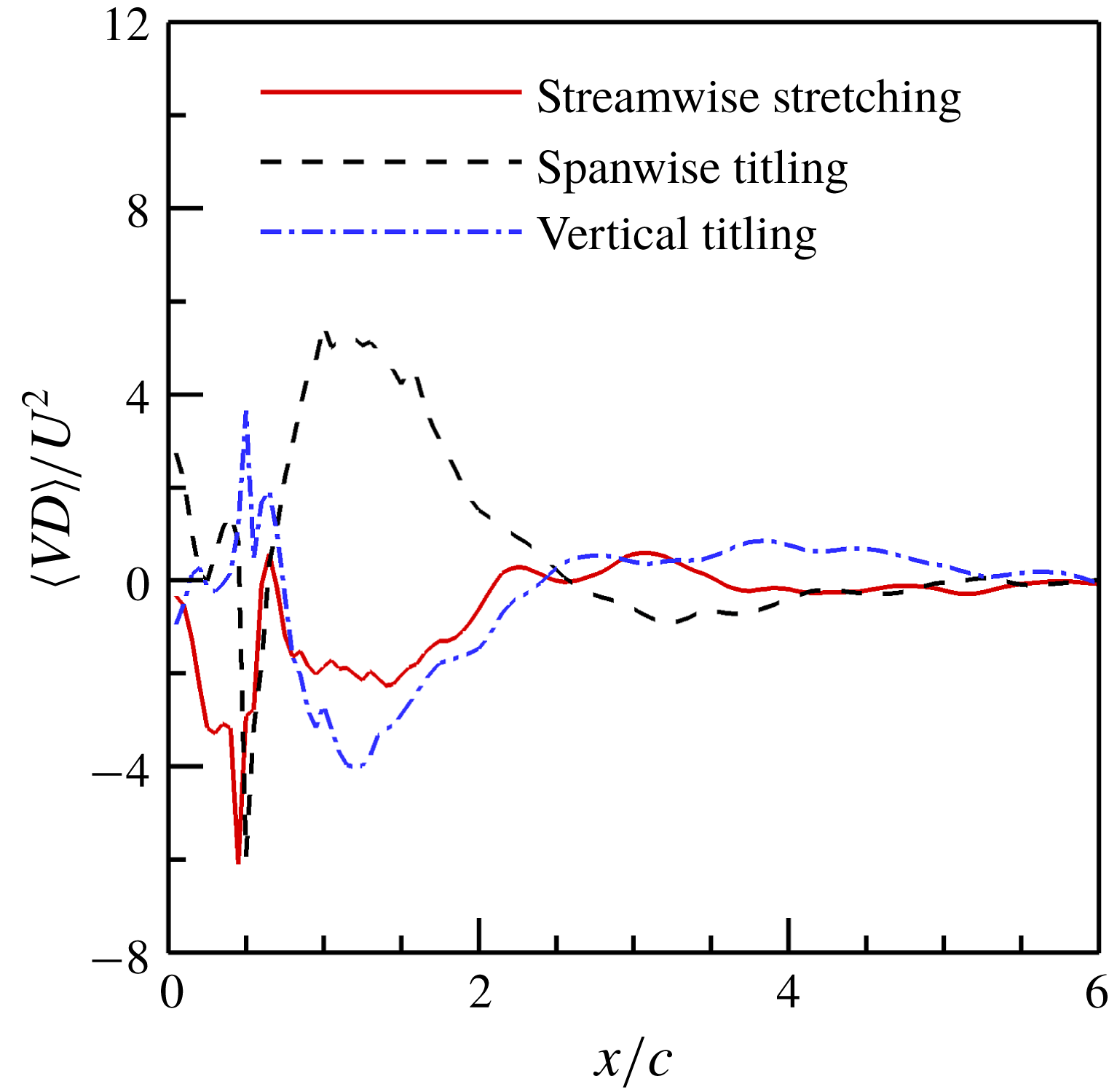
The vortex deformation revealed in figure 5 can be quantitatively described by the vortex stretching integrated in the wake plane, and thus the vortex deformation parameter for the streamwise vorticity (VD) is introduced as
 $$\begin{eqnarray}\displaystyle VD=\int _{S^{+}(X)}\left(\unicode[STIX]{x1D714}_{x}\frac{\unicode[STIX]{x2202}u_{x}}{\unicode[STIX]{x2202}x}+\unicode[STIX]{x1D714}_{y}\frac{\unicode[STIX]{x2202}u_{x}}{\unicode[STIX]{x2202}y}+\unicode[STIX]{x1D714}_{z}\frac{\unicode[STIX]{x2202}u_{x}}{\unicode[STIX]{x2202}z}\right)\text{d}S, & & \displaystyle\end{eqnarray}$$
which measures the interaction between the vorticity and the gradient of the streamwise velocity in the Trefftz plane. The subscripts in (3.3) indicate the vector components in
 $x$
-,
 $y$
- and
 $z$
-directions, respectively. The first, second and third terms of the integral in (3.3) represent the increase of the streamwise vorticity contributed by the stretching of the streamwise vortex, tilting of the spanwise vorticity, and the tilting of the vertical vorticity, respectively. The time-averaged values of the three terms are shown in figure 6. Clearly, the tilting of the spanwise vorticity mainly contributes to the increase of the streamwise vorticity, while the tilting of the vertical vorticity causes the decrease of the streamwise vorticity. The stretching of the streamwise vorticity contributes to the increase of the streamwise vorticity in the near wake and the decrease of the streamwise vorticity in the middle wake. Similar parameters can be defined for the convection term and diffusion term of the vorticity dynamic equations. The superposition of all the terms does not result in a zero change rate, which indicates that the circulation estimated in the Trefftz plane is not conserved. Thus, the constant wingspan cannot be used for the flapping wing model as the effective span length in (2.1). To obtain the correct time-averaged lift independent of the location of the Trefftz plane, the correct effective span length should change inversely with the circulation.
Time-averaged vortex deformation parameter for the flapping rectangular wing with a fixed wingspan.

The DPV in the Trefftz plane has been used to take into account the three-dimensional effect (Muijres et al.
Reference Muijres, Bowlin, Johansson and Hedenstrom2012; Gutierrez et al.
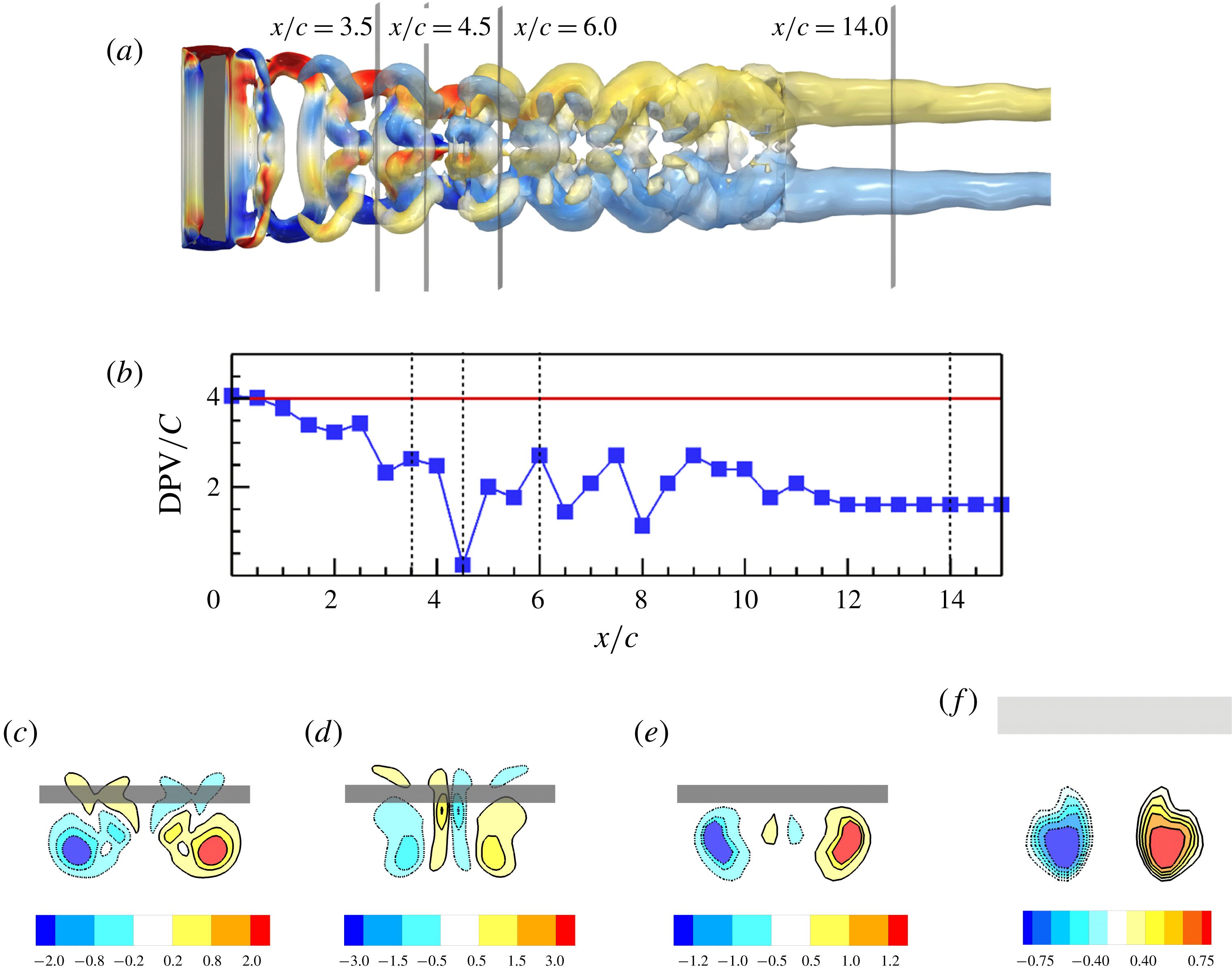
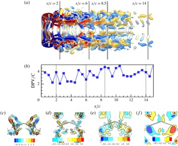
Reference Gutierrez, Quinn, Chin and Lentink2016). However, this approach usually gives a puzzling result because the distribution of the streamwise vorticity in the Trefftz plane is not fully taken into account. The wake vortex structures at the middle of the downstroke and the DPV at different Trefftz planes are shown in figure 7. The DPV varies with the streamwise position of the Trefftz plane, especially in the middle wake (from
 $x/c\approx 3.0$
to
 $x/c\approx 10.0$
), where the vortex rings deform and interact with each other. The complex interactions between the vortex structures generated by the flapping wing may lead to abrupt positional changes of the vorticity peaks. The deformation of the vortex rings might cause very close peaks of the streamwise vorticity, as shown in figure 7(d), where the peak streamwise vorticity corresponding to the highly curved vortex rings causes a near-zero wake width (
 $\text{DPV}=0.27$
) at
 $x/c=4.5$
. While, at a short distance in the downstream (
 $x/c=6.0$
), the DPV is approximately 2.7, which is 10 times as large as that at
 $x/c=4.5$
. Besides the poor performance in the middle-wake region, the DPV also does not give the correct prediction of the time-averaged lift coefficient even in the near- and far-wake regions where the wake width changes gently. This is because the DPV just reflects the positions of the streamwise vorticity peaks and cannot take into account the various distributions of the streamwise vorticity in different Trefftz planes. For example, the DPV cannot tell the difference between figure 7(c) and 7(e), where the DPVs are almost the same in the two Trefftz planes while the distributions of the vorticity are very different.
Flow structures and wake width of the flapping rectangular wing with a fixed wingspan: (a) top view of the isosurfaces of
 $Q=0.2$
, coloured by the normalized spanwise vorticity from
 $-1$
(blue) to 1 (red); (b) the DPV in 31 different Trefftz planes; and (c–f) streamwise vorticity fields at
 $x/c=3.5$
,
 $x/c=4.5$
,
 $x/c=6.0$
and
 $x/c=14.0$
, respectively.

The distinct feature of the wake of this flapping wing is that the wake width decreases to an asymptotic value. The decrease of wake width has also been reported in other flapping wing models for bio-inspired swimming (Blondeaux et al.
Reference Blondeaux, Fornarelli, Guglielmini, Triantafyllou and Verzicco2005; Buchholz & Smits Reference Buchholz and Smits2005; Dong, Mittal & Najjar Reference Dong, Mittal and Najjar2006). The narrowing wake width is caused by the mutually induced motion of the TVs (Dong et al.
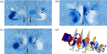
Reference Dong, Mittal and Najjar2006), as shown in figure 8(a). In addition, the self-induced motion of the deformed vortex rings also tends to reduce the wake width, as shown in figure 8(b) where the vorticity in the plane
 $x/c=2.75$
comes from the same vortex ring. The self- and mutually induced motions could be combined at certain locations, as shown in figure 8(c). The VWW of the wake gives a good prediction of the spanwise narrowing process, as shown in figure 3(c). Although the time-averaged DPV varies with the locations of the Trefftz planes, as shown in figure 3(c), it cannot correctly represent the wake narrowing and does not vary inversely with the circulation. In contrast, the VWW defined in (2.6) gives a correct wake width to compensate the variation of the circulation in the wake, as shown in figure 3(b).
The induced motion of vortices in the wake at different streamwise positions, where the (purple) solid arrows show the direction of induced motion: (a) the mutually induced motion caused by the tip vortices,
 $x/c=1.65$
; (b) the self-induced motion caused by the deformation of vortex ring,
 $x/c=2.75$
; (c) the combination of the mutually and self-induced motions,
 $x/c=4.0$
; and (d) the positions of the slices interacting with the vortex structures at
 $x/c=1.65$
, 2.75 and 4.0, respectively.

The time-dependent lift coefficients predicted by using the KJ theorem in different Trefftz planes for the flapping wing with a dynamically changing wingspan. The wingspan is taken as the effective span length in computing the KJ lift.

(a) Time-averaged lift coefficients based on the KJ theorem with different effective span lengths; (b) time-averaged circulation and moment of the vorticity in different Trefftz planes; and (c) time-averaged wake width computed by different methods for the flapping wing with a dynamically changing wingspan.

Time-averaged vortex deformation parameter computed by different methods for the flapping rectangular wing with a dynamically changing wingspan.

4 Flapping wing with a dynamically changing wingspan
4.1 The Kutta–Joukowski lift
We further investigate the applicability of the KJ theorem to the flapping wing with a dynamically changing wingspan, where the spanwise stretching and retracting motion is superimposed onto the flapping kinematics described by (3.1) and (3.2). The flapping wing with a dynamically changing wingspan has been employed by Wang et al. (Reference Wang, Zhang, He and Liu2014) to simulate the changing of the wingspan in the flapping flight of a bird and bat, where the wing stretches outwards in the downstroke and retracts towards the body in the upstroke. A similar model was used by Guan & Yu (Reference Guan and Yu2015) to investigate the mechanisms of morphing wings in forward flight of a bat. The dynamically changing wingspan in this case is described by the aspect ratio (
 $AR$
) as
 $$\begin{eqnarray}\displaystyle AR=b/c=AR_{0}(a_{1}-a_{2}\sin (2\unicode[STIX]{x03C0}ft+\unicode[STIX]{x1D719})), & & \displaystyle\end{eqnarray}$$
where
 $AR_{0}=b_{0}/c$
is the characteristic aspect ratio,
 $b_{0}=4c$
is the characteristic wingspan,
 $a_{1}=0.75$
and
 $a_{2}=0.25$
are the coefficients that specify the stretching and retracting amplitude, and
 $\unicode[STIX]{x1D719}=\unicode[STIX]{x03C0}/2$
is the phase difference between the flapping and stretching/retracting motion. The time-averaged wingspan is 3.0. The other geometrical and kinematical parameters in the simulation are the same as those in § 3.
When the dynamic wingspan is used for the effective span length in (2.2), as shown in figure 9, the time-dependent lift coefficients obtained in three different locations of the Trefftz plane are similar to those in the fixed wingspan case. The KJ lift underpredicts both the positive and negative peaks of the lift coefficient, and the peaks of the lift coefficient decrease as the Trefftz plane moves downstream. Therefore, the KJ theorem with the wingspan as the effective span length cannot give the correct prediction of the unsteady lift of this flapping wing. Furthermore, the selection of the DPV as the effective span length fails to predict the unsteady lift coefficient.
Figure 10(a) shows the time-averaged lift coefficient evaluated as a function of the locations of the Trefftz plane. When the wingspan is selected as the effective span length in (2.2), the time-averaged lift is slightly underpredicted in the near wake and considerably overpredicted in the middle and far wake, which depends strongly on the location of the Trefftz plane. The maximum time-averaged lift coefficient is approximately 190 % of the DNS value. In contrast, when the DPV is selected as the effective span length, the result is much improved. The maximum time-averaged lift coefficient is approximately 130 % of the DNS value. The relatively good performance of DPV is related to the stronger lower branch of the wake, as discussed in § 4.2. Despite the fortunate improvement in this case, the result still depends on the location of the Trefftz plane. In contrast, the WS-KJ model with the VWW can resolve this problem, as shown in figure 10(a).
The time-averaged circulation varies with the location of the Trefftz plane, as shown in figure 10(b). The variation of the time-averaged circulation is related to the evolution of the vortex rings originated from the LEVs, TVs and TEVs. In contrast to the time-averaged circulation, the time-averaged vorticity moment in the Trefftz plane remains largely constant. Figure 10(c) shows the effective span lengths as a function of the location of the Trefftz plane. Interestingly, the DPV exhibits almost the same behaviour as the VWW. This explains why the selection of the DPV luckily leads to the improved result in this special case. The relatively simple vortex deformation and interactions can be quantitatively measured by the vortex deformation parameter shown in figure 11, which are smoother than that for the fixed wing case in figure 6 in the middle-wake region.
To examine the applicability of the KJ theorem to estimation of the unsteady lift, the lift is decomposed into the vortex force and the local fluid acceleration term according to (2.7). As shown in figure 12(a), the vortex force mainly contributes the time-averaged value of the lift, while the local fluid acceleration term dominates the phase and amplitude of the lift. Comparison of the KJ lift estimated in the Trefftz plane at
 $x/c=1.0$
with the vortex lift is shown in figure 12(b), indicating that the KJ lift in the near wake approximately recovers the vortex lift. However, the KJ theorem cannot fully incorporate the phase information associated with the local fluid acceleration. Similar to the procedure discussed in § 3, the added-mass force model can be used to approximately evaluate the local fluid acceleration term in this case. The results support the conclusion that the KJ lift model with the quasi-steady assumption is not applicable to the current flapping wing. The added-mass effect should be considered to correctly estimate the instantaneous lift.
(a) The decomposition of the lift coefficient by using (2.7); and (b) the KJ lift, added-mass lift and their comparisons with the decomposed lift in the flow over the flapping rectangular wing with a dynamically changing wingspan.

Wake structures of the flapping rectangular wing with a dynamically changing wingspan at the middle of the upstroke: (a) top view and (b) side view. The vortex structures are identified by using the isosurfaces of
 $Q=0.2$
and coloured by the normalized spanwise vorticity from
 $-5$
(blue) to 5 (red).

Flow structures and wake width of the flapping rectangular wing with a dynamically changing wingspan at the middle of the downstroke: (a) top view of the isosurfaces of
 $Q=0.2$
coloured by the streamwise vorticity from
 $-1$
(blue) to 1 (red); (b) the DPV in 31 different Trefftz planes; and (c–f) streamwise vorticity fields at
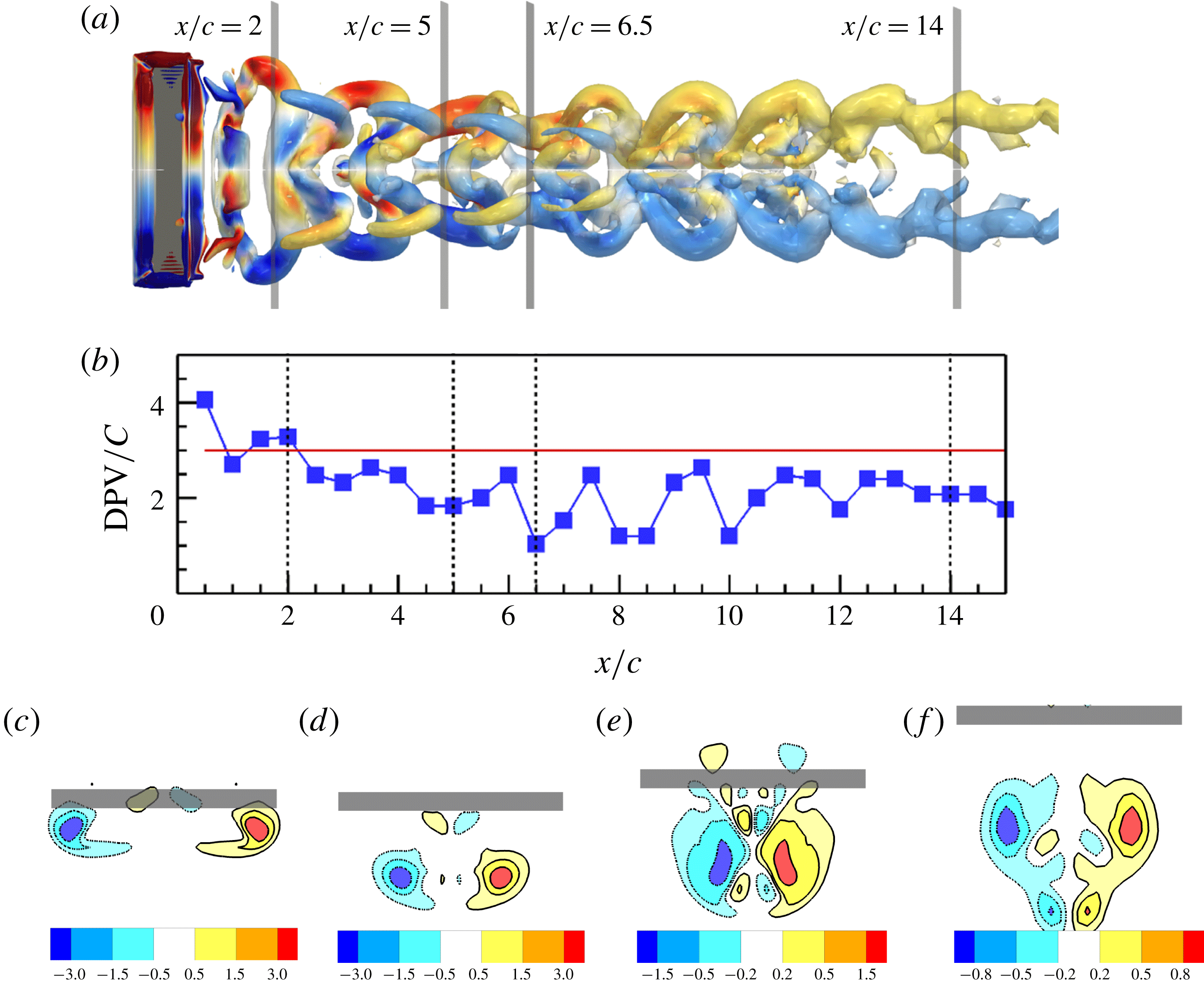
 $x/c=2.0$
,
 $x/c=5.0$
,
 $x/c=6.5$
and
 $x/c=14.0$
, respectively.

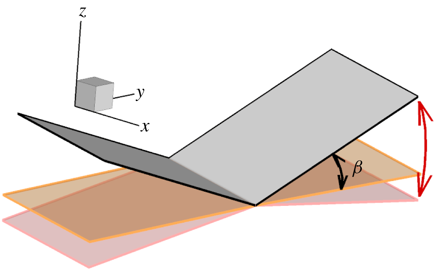
Schematic of the dihedral flapping wing.

4.2 Wake vortex structures
The typical wake structures of the flapping wing with a dynamically changing wingspan are shown in figure 13. The flapping wing generates a pair of vortex rings in each flapping period, which originate from the LEV, TVs and TEV. The vortex rings deform and interact with each other as they convect downstream. The topology and evolution of the wake vortex structures are similar to those reported in § 3. The main difference between the fixed wingspan case and the dynamically changing wingspan case is that the dynamically changing wingspan case generates asymmetric wakes, where the vortex ring generated in the downstroke is much stronger than the one generated in the upstroke due to the spanwise stretching/retracting motion. The generation of the asymmetric vortex rings results in the lower branch of the vortices in the middle wake that is much stronger than the upper branch. The stronger lower branch of the vortices leads to a pair of dominant vortex structures in the Trefftz planes, as shown in figure 14(c–f). More details of the generation and evolution of the vortex structures generated by this flapping wing can be found in our previous work (Wang et al. Reference Wang, Zhang, He and Liu2014).
5 Dihedral flapping wing
5.1 The Kutta–Joukowski lift
Compared to the relatively well-organized TVs generated by the flapping wing models in §§ 3 and 4, a dihedral flapping wing model can generate more complex wake vortex structures. The dihedral flapping wing model consists of a pair of rectangular wings that rotate dynamically around the symmetry axis. Here, the term ‘dihedral wing’ is extended to describe this flapping wing with periodically changing dihedral angle (the rotational angle) between a positive value and a negative value. The schematic of this dihedral flapping wing is shown in figure 15. A dihedral flapping wing was employed by Kim, Hussain & Gharib (Reference Kim, Hussain and Gharib2013) and Suzuki, Minami & Inamuro (Reference Suzuki, Minami and Inamuro2015) to investigate the aerodynamics of a butterfly. Hu, Clemons & Igarashi (Reference Hu, Clemons and Igarashi2011) used a dihedral flapping wing as a bio-inspired micro-air vehicle (MAV) model to investigate unsteady vortex structures. In this case, the heaving motion described in (3.2) is replaced by the rotational angle around the wing symmetry axis, which is given by
 $$\begin{eqnarray}\displaystyle \unicode[STIX]{x1D6FD}(t)=\unicode[STIX]{x1D6FD}_{0}+\unicode[STIX]{x1D6FD}_{m}\cos (2\unicode[STIX]{x03C0}ft), & & \displaystyle\end{eqnarray}$$
where
 $\unicode[STIX]{x1D6FD}$
is the angle between the semi-wingspan and the horizontal plane, and
 $\unicode[STIX]{x1D6FD}_{0}=0^{\circ }$
and
 $\unicode[STIX]{x1D6FD}_{m}=20^{\circ }$
are the time-averaged rotational angle and the rotational angle amplitude, respectively. In this simulation, the pitching motion is turned off by setting the pitching amplitude
 $\unicode[STIX]{x1D6FC}_{m}=0$
in (3.1). The maximum wingspan is 4.0 and the other geometrical and kinematical parameters are the same as those in § 3.
Figure 16 presents the time-dependent lift coefficients evaluated in three different Trefftz planes with the maximum wingspan as the effective span length. The KJ lift coefficient has a phase difference from the DNS lift, which is similar to the results reported in §§ 3 and 4. In particular, the lift peaks predicted by the KJ theorem are much smaller than the DNS lift. The peaks of the DNS lift are almost three times as large as those in §§ 3 and 4. This is because the kinematics given by (5.1) gives the maximum flapping amplitude of
 $0.68c$
, which is approximately three times (2.72 times) as large as the heaving amplitude of the models in §§ 3 and 4. The large flapping amplitude of the dihedral flapping wing causes a large acceleration of the fluid around it. The contribution of the local acceleration of fluid to the lift can be clearly seen in figure 17(a), where the peaks of the lift are dominated by
 $L_{acc}$
. Note that geometry and kinematics of the current dihedral flapping wing model are designed to generate complex wake structures other than the optimal aerodynamic performance. The peaks of the KJ lift are much smaller than the vortex lift even in the near wake, as shown in figure 17(b), which is different from the cases in §§ 3 and 4.
The time-dependent lift coefficients predicted by using the KJ theorem in different Trefftz planes for the dihedral flapping wing. The maximum wingspan is taken as the effective span length in computing the KJ lift.

(a) The decomposition of the lift coefficients by using (2.7); and (b) the KJ lift at different Trefftz planes and their comparisons with the vortex lift in the flow over the dihedral flapping wing.

(a) Time-averaged lift coefficient based on the KJ theorem with different effective span lengths; (b) time-averaged circulation and moment of the vorticity in different Trefftz planes; and (c) time-averaged wake width computed by different methods for the dihedral flapping wing.

Time-averaged vortex deformation parameter for the dihedral flapping wing.

Typical vortex structures generated by the dihedral flapping wing at the middle of the downstroke: (a) top view and (b) side view, where the isosurfaces of
 $Q=1.0$
are shown. The colour shows the spanwise vorticity from
 $-5$
(blue) to 5 (red).

Flow structures and wake width of the dihedral flapping wing: (a) top view of the isosurfaces of
 $Q=0.2$
coloured by the streamwise vorticity from
 $-1$
(blue) to 1 (red); (b) the DPV in 31 different Trefftz planes; and (c–f) streamwise vorticity fields at
 $x/c=2.0$
,
 $x/c=6.0$
,
 $x/c=8.5$
and
 $x/c=14.0$
, respectively.

The time-averaged lift coefficients are shown in figure 18(a). When the maximum wingspan is used as the effective span length, the KJ lift overpredicts the time-averaged lift coefficient. The time-averaged KJ lift coefficient increases with the location of the Trefftz plane. The maximum time-averaged KJ lift coefficient is approximately 150 % of the DNS lift. In contrast, when the DPV is selected as the effective span length, the time-averaged KJ lift gives an underprediction in the near wake (
 $x/c<6.0$
) and an overprediction in the middle and far wake (
 $x/c>6.0$
). The minimum and maximum time-averaged KJ lift coefficients are approximately 70 % and 120 % of the DNS values. The time-averaged DPV does not vary inversely with the circulation, as shown in figure 18(b). When the WS-KJ model with the VWW is used, the time-averaged KJ lift agrees well with the DNS lift. The difference between the KJ lift and the truth is within 7 % in most Trefftz planes. As as shown in figure 18(b), the time-averaged VWW effectively compensates the variation of the circulation in the wake. The variations of the effective span lengths are shown in figure 18(c). The complex interaction of the vortex structures in the near wake can be reflected by the vortex deformation parameter shown in figure 19, where both the stretching and tilting terms are much larger than those for other wings.
5.2 Wake vortex structures
Compared to the flapping rectangular wings with fixed and dynamically changing wingspans discussed in §§ 3 and 4, the wake vortex structures of the dihedral flapping wing are much more complex, as shown in figure 20. The TVs deform immediately after they are shed from the wingtips, interacting with the LEV and TEV. Then, the highly deformed TVs tangle with different structures. Neither apparent vortex rings nor distinct wake regions can be identified. The spanwise narrowing of the wake width is also not apparent. As shown in figure 21, the distributions of the streamwise vorticity in the Trefftz planes are much more complex than those in figures 7 and 14. There is no dominant vortex structure in the Trefftz planes. In this case, the VWW is the only rational choice for the effective wake length.
6 Conclusions
The applicability of the KJ theorem in lift estimation based on the wake velocity fields at the Trefftz planes is examined for flapping wings with fixed and dynamically changing wingspans and the dihedral flapping wing through numerical simulations of viscous incompressible flows. It is found that the KJ theorem under the quasi-steady assumption cannot predict the unsteady lift in both the magnitude and phase from the wake velocity fields. The KJ theorem recovers approximately the vortex lift, but does not incorporate the fluid acceleration effect that dominates the unsteady lift. In principle, the time-averaged KJ theorem can predict the time-averaged lift when the effective span length of the wake is rationally selected. We propose a WS-KJ model where the effective span length is computed by a vorticity-weighted width. The vorticity-weighted width represents the spanwise distance between the streamwise vorticity centroids in the right and left half sides of the Trefftz plane. The WS-KJ model naturally incorporates the effects of the evolving vortex structures in the Trefftz planes. For the steady flows over wings with a pair of parallel straight vortex lines or tubes, the WS-KJ model reduces to the classical aerodynamic model. Indeed, the WS-KJ model is able to give a good prediction of the time-averaged lift despite the complex wake vortex structures in flapping flight. The circulation estimated in the Trefftz plane is highly related to the interactions of the complex vortex structures in the wake. Interestingly, this spatial evolutionary effect of the estimated circulation can be compensated by using the vorticity-weighted width such that the time-averaged total vorticity moment is formally conserved in the wake. In contrast, the heuristic selections of the effective span length such as the wingspan and the distance between the peaks of the DPV cannot give the correct time-averaged lift, and the results are highly dependent on the locations of the Trefftz planes. Furthermore, for a flapping wing with relatively simple geometry and kinematics, the fluid acceleration effect can be modelled by an added-mass force model. In this case, superposition of the instantaneous KJ lift and the added-mass lift gives a reasonable approximation of the unsteady lift.
Acknowledgements
This work was supported by the National Natural Science Foundation of China (grant nos 91752118, 11672305, 11232011 and 11572331). The authors would like to acknowledge the support from the Strategic Priority Research Programme grant no. XDB22040104 and Key Research Programme of Frontier Sciences of the Chinese Academy of Sciences (grant no. QYZDJ-SSW-SYS002). T.L. would like to acknowledge the hospitality received at LNM during his visit where he accomplished this work. The computations are conducted on Tianhe-1 at the National Supercomputer Centre in Tianjin.
Appendix A. Vortex lift and vorticity moment in the Trefftz plane
The vortex lift can be expressed as the total vorticity moment in the Trefftz plane receding to infinity downstream (as
 $X\rightarrow \infty$
). The derivation of this result is given as follows. The vortex lift is given by
 $$\begin{eqnarray}\displaystyle L_{vor}=\unicode[STIX]{x1D70C}\boldsymbol{k}\boldsymbol{\cdot }\int _{V_{f}}\boldsymbol{u}\times \unicode[STIX]{x1D74E}\,\text{d}V, & & \displaystyle\end{eqnarray}$$
where
 $\boldsymbol{k}$
is the unit vector normal to the free-stream velocity,
 $\boldsymbol{u}$
and
 $\unicode[STIX]{x1D74E}=\unicode[STIX]{x1D735}\times \boldsymbol{u}$
are the velocity and vorticity, respectively,
 $\unicode[STIX]{x1D70C}$
is the fluid density, and
 $V_{f}$
is the fluid control volume. The velocity can be decomposed as
 $$\begin{eqnarray}\displaystyle \boldsymbol{u}\equiv \boldsymbol{U}+\boldsymbol{u}^{\prime }, & & \displaystyle\end{eqnarray}$$
where
 $\boldsymbol{U}=(U,0,0)$
is the background flow,
 $U$
is the free-stream velocity magnitude, and
 $\boldsymbol{u}^{\prime }$
is the perturbation velocity induced by the vortex structures and added-mass effect. We have
 $\unicode[STIX]{x1D735}\times \boldsymbol{u}=\unicode[STIX]{x1D735}\times \boldsymbol{u}^{\prime }$
since
 $\boldsymbol{U}$
is uniform in the domain.
Schematic of the integral domain for the vortex force.

The integral of the Lamb vector term in (A 1) can be expressed as follows:
 $$\begin{eqnarray}\displaystyle \int _{V_{f}}\boldsymbol{u}\times \unicode[STIX]{x1D74E}\,\text{d}V=\int _{V_{f}}\boldsymbol{U}\times \unicode[STIX]{x1D74E}\,\text{d}V+\int _{V_{f}}\boldsymbol{u}^{\prime }\times \unicode[STIX]{x1D74E}\,\text{d}V. & & \displaystyle\end{eqnarray}$$
The first term on the right-hand side of (A 3) is given by
 $$\begin{eqnarray}\displaystyle \int _{V_{f}}\boldsymbol{U}\times \unicode[STIX]{x1D74E}\,\text{d}V=\boldsymbol{U}\times \int _{V_{f}}\unicode[STIX]{x1D74E}\,\text{d}V=\boldsymbol{U}\times \int _{\unicode[STIX]{x2202}V_{f}}\boldsymbol{x}(\boldsymbol{n}\boldsymbol{\cdot }\unicode[STIX]{x1D74E})\,\text{d}S, & & \displaystyle\end{eqnarray}$$
where
 $\unicode[STIX]{x2202}V_{f}$
denotes the boundary of the integral volume. The derivative–moment transformation (Wu et al.
Reference Wu, Ma and Zhou2006)
 $$\begin{eqnarray}\displaystyle \int _{V}\unicode[STIX]{x1D74E}\,\text{d}V=-\int _{V}\boldsymbol{x}(\unicode[STIX]{x1D735}\boldsymbol{\cdot }\unicode[STIX]{x1D74E})\,\text{d}V+\int _{\unicode[STIX]{x2202}V}\boldsymbol{x}(\boldsymbol{n}\boldsymbol{\cdot }\unicode[STIX]{x1D74E})\,\text{d}S, & & \displaystyle\end{eqnarray}$$
and the identity
 $\unicode[STIX]{x1D735}\boldsymbol{\cdot }\unicode[STIX]{x1D74E}=0$
are used in the derivation of (A 4). For the integral volume shown in figure 22 with the right boundary being at the Trefftz plane (
 $x=X$
), the contribution of (A 4) to lift is
 $$\begin{eqnarray}\displaystyle \boldsymbol{k}\boldsymbol{\cdot }\int _{V_{f}}\boldsymbol{U}\times \unicode[STIX]{x1D74E}\,\text{d}V=\boldsymbol{k}\boldsymbol{\cdot }\left(\boldsymbol{U}\times \int _{\unicode[STIX]{x2202}V_{f}}\boldsymbol{x}(\boldsymbol{n}\boldsymbol{\cdot }\unicode[STIX]{x1D74E})\,\text{d}S\right)=U\int _{x=X}y\unicode[STIX]{x1D714}_{x}\,\text{d}S. & & \displaystyle\end{eqnarray}$$
The second term on the right-hand side of (A 3) is written as
 $$\begin{eqnarray}\displaystyle \int _{V_{f}}\boldsymbol{u}^{\prime }\times \unicode[STIX]{x1D74E}\,\text{d}V & = & \displaystyle \int _{V_{f}}\left(\unicode[STIX]{x1D735}\left(\frac{\boldsymbol{u}^{\prime }\boldsymbol{\cdot }\boldsymbol{u}^{\prime }}{2}\right)-\unicode[STIX]{x1D735}\boldsymbol{\cdot }(\boldsymbol{u}^{\prime }\boldsymbol{u}^{\prime })\right)\text{d}V\nonumber\\ \displaystyle & = & \displaystyle \int _{\unicode[STIX]{x2202}V_{f}}\boldsymbol{n}\left(\frac{\boldsymbol{u}^{\prime }\boldsymbol{\cdot }\boldsymbol{u}^{\prime }}{2}\right)\text{d}S-\int _{\unicode[STIX]{x2202}V_{f}}\boldsymbol{n}\boldsymbol{\cdot }(\boldsymbol{u}^{\prime }\boldsymbol{u}^{\prime })\,\text{d}S,\end{eqnarray}$$
where
 $\boldsymbol{n}$
is the unit vector normal to the boundary
 $\unicode[STIX]{x2202}V_{f}$
. The Gaussian theorem is used in (A 7) with the incompressibility constraint
 $\unicode[STIX]{x1D735}\boldsymbol{\cdot }\boldsymbol{u}^{\prime }=0$
and the vector identity
 $$\begin{eqnarray}\displaystyle \boldsymbol{u}^{\prime }\times \unicode[STIX]{x1D74E}=\unicode[STIX]{x1D735}\left(\frac{\boldsymbol{u}^{\prime }\boldsymbol{\cdot }\boldsymbol{u}^{\prime }}{2}\right)-\unicode[STIX]{x1D735}\boldsymbol{\cdot }(\boldsymbol{u}^{\prime }\boldsymbol{u}^{\prime }). & & \displaystyle\end{eqnarray}$$
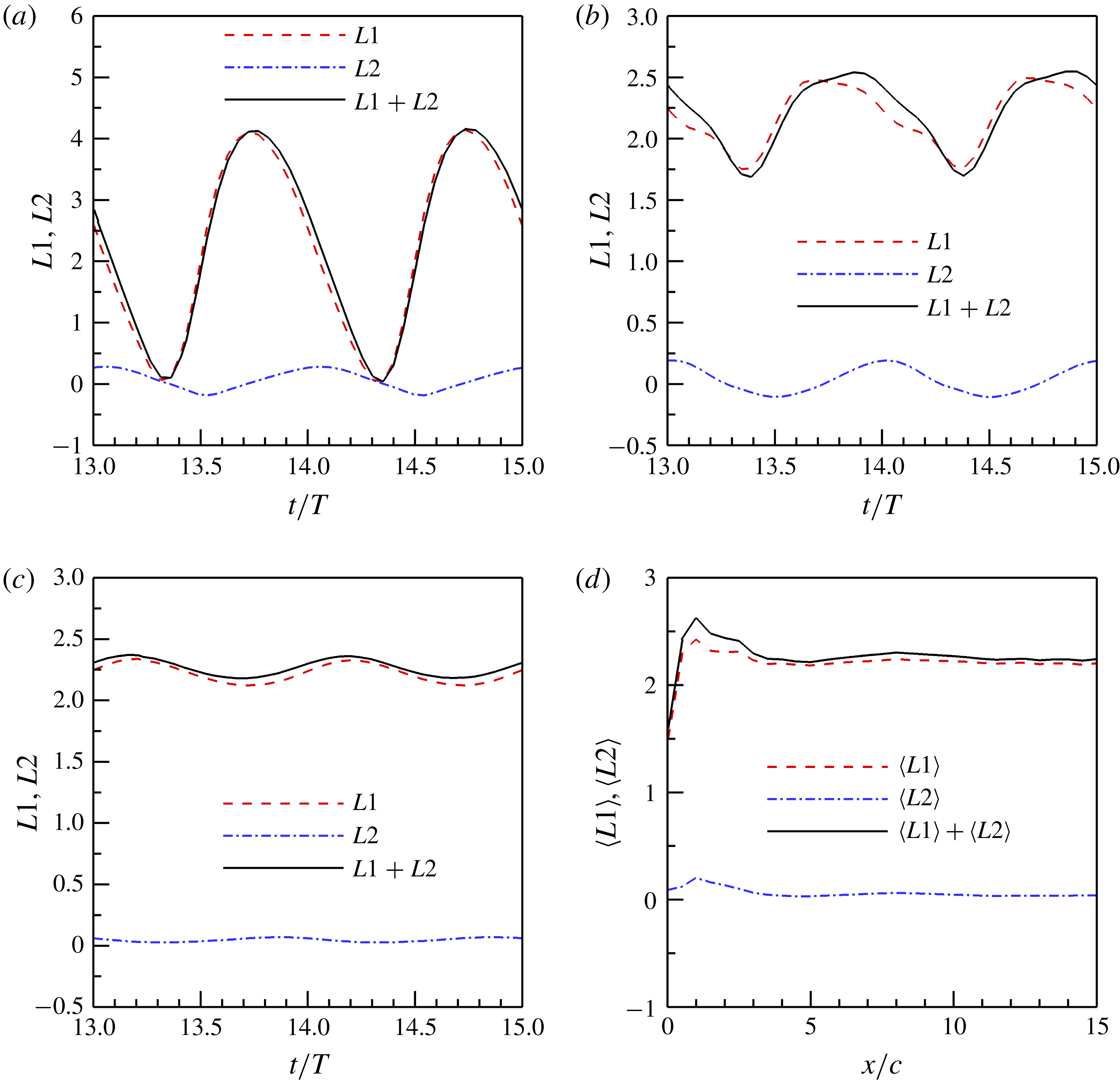
Contributions from (A 6) to (A 10), denoted by
 $L1$
and
 $L2$
, respectively, for the flapping rectangular wing with a fixed wingspan in different Trefftz planes: (a–c) time-dependent lift at
 $x/c=3.0$
,
 $x/c=5.0$
and
 $x/c=10.0$
, respectively; and (d) time-averaged lift. The
 $L1$
and
 $L2$
are normalized by
 $\unicode[STIX]{x1D70C}U^{2}c^{2}$
.

The contribution of (A 7) to the lift is given as
 $$\begin{eqnarray}\displaystyle \boldsymbol{k}\boldsymbol{\cdot }\int _{V_{f}}\boldsymbol{u}^{\prime }\times \unicode[STIX]{x1D74E}\,\text{d}V & = & \displaystyle \boldsymbol{k}\boldsymbol{\cdot }\int _{\unicode[STIX]{x2202}V_{f}}\boldsymbol{n}\left(\frac{\boldsymbol{u}^{\prime }\boldsymbol{\cdot }\boldsymbol{u}^{\prime }}{2}\right)\text{d}S-\boldsymbol{k}\boldsymbol{\cdot }\int _{\unicode[STIX]{x2202}V_{f}}\boldsymbol{n}\boldsymbol{\cdot }(\boldsymbol{u}^{\prime }\boldsymbol{u}^{\prime })\,\text{d}S\nonumber\\ \displaystyle & = & \displaystyle \int _{\unicode[STIX]{x2202}V_{f}}q^{2}\boldsymbol{n}\boldsymbol{\cdot }\boldsymbol{k}\,\text{d}S-\int _{\unicode[STIX]{x2202}V_{f}}u_{n}u_{k}\,\text{d}S,\end{eqnarray}$$
where
 $q^{2}=\boldsymbol{u}^{\prime }\boldsymbol{\cdot }\boldsymbol{u}^{\prime }/2$
is the dynamic pressure contributed by the velocity fluctuations, and
 $u_{n}$
and
 $u_{k}$
are the velocity components along the normal direction of the boundary and the vertical direction to the incoming flow, respectively. For a sufficiently large but finite rectangular control volume with a Trefftz plane in the wake shown in figure 22, the lifts contributed by the velocity fluctuations on the top and bottom (or front and back in three-dimensional flows) surfaces cancel with each other because of the opposite sign of the normal vectors. Therefore, equation (A 9) can be approximated by the term in the Trefftz plane in the wake, i.e.
 $$\begin{eqnarray}\displaystyle \boldsymbol{k}\boldsymbol{\cdot }\int _{V_{f}}\boldsymbol{u}^{\prime }\times \unicode[STIX]{x1D74E}\,\text{d}V\approx -\int _{x=X}u_{n}u_{k}\,\text{d}S. & & \displaystyle\end{eqnarray}$$
Equation (A 10) approaches zero as
 $|\boldsymbol{X}|\rightarrow \infty$
, since the integral of (A 10) is taken over a finite rectangular domain on the Trefftz plane and the velocity fluctuations decay to zero as
 $|\boldsymbol{X}|\rightarrow \infty$
. The asymptotic form of the vortex lift as
 $|\boldsymbol{X}|\rightarrow \infty$
(or (2.11) in § 2) can be approximated by:
 $$\begin{eqnarray}\displaystyle L_{vor}\approx U\int _{x=X}y\unicode[STIX]{x1D714}_{x}\,\text{d}s. & & \displaystyle\end{eqnarray}$$
Thus, the time-averaged vortex lift is
 $$\begin{eqnarray}\displaystyle \langle L_{vor}\rangle \approx \unicode[STIX]{x1D70C}U\left\langle \int _{S^{+}(X)}y\unicode[STIX]{x1D714}_{x}\,\text{d}S\right\rangle =\unicode[STIX]{x1D70C}U\langle b_{vor}(t,X)\rangle \langle \unicode[STIX]{x1D6E4}(t,X)\rangle , & & \displaystyle\end{eqnarray}$$
where
 $\langle \bullet \rangle =(1/T)\int _{t_{0}}^{t_{0}+T}\bullet \,\text{d}t$
is the time-averaged operator and
 $T$
is the flapping period. The terms
 $\langle b_{vor}(t,X)\rangle$
and
 $\langle \unicode[STIX]{x1D6E4}(t,X)\rangle$
are defined as
 $$\begin{eqnarray}\displaystyle & \displaystyle \langle b_{vor}\rangle =2\frac{\left\langle \displaystyle \int _{S^{+}(X)}y\unicode[STIX]{x1D714}_{x}(t^{\prime })\,\text{d}S\right\rangle }{\left\langle \displaystyle \int _{S^{+}(X)}\unicode[STIX]{x1D714}_{x}(t^{\prime })\,\text{d}S\right\rangle }=\frac{\left\langle \displaystyle \int _{S(X)}y\unicode[STIX]{x1D714}_{x}(t^{\prime })\,\text{d}S\right\rangle }{\left\langle \displaystyle \int _{S^{+}(X)}\unicode[STIX]{x1D714}_{x}(t^{\prime })\,\text{d}S\right\rangle }, & \displaystyle\end{eqnarray}$$
 $$\begin{eqnarray}\displaystyle & \displaystyle \langle \unicode[STIX]{x1D6E4}(t,X)\rangle =\left\langle \int _{S^{+}(X)}\unicode[STIX]{x1D714}_{x}(t^{\prime })\,\text{d}S\right\rangle , & \displaystyle\end{eqnarray}$$
where
 $S^{+}(X)$
is the right-hand side of the Trefftz plane at
 $x=X$
,
 $S(X)=S^{+}(X)+S^{-}(X)$
is the entire Trefftz plane,
 $\unicode[STIX]{x1D714}_{x}$
is the streamwise component of the vorticity, and
 $t^{\prime }$
is the time when the vorticity is measured in the Trefftz plane at
 $x=X$
. The relation between the time when the force acts on the wing and the delayed time is
 $$\begin{eqnarray}\displaystyle t=t^{\prime }-\frac{X-x_{t}}{U_{conv}}. & & \displaystyle\end{eqnarray}$$
It is noted that there are different ways to derive (A 11), such as the work of Wu (Reference Wu1981), Wu et al. (Reference Wu, Ma and Zhou2006) and Wu et al. (Reference Wu, Liu and Liu2018). For the Trefftz plane at a finite distance (
 $x=X$
), the correlation term
 $\langle u_{n}u_{k}\rangle$
of the velocity fluctuations in (A 10) may contribute to
 $\langle L_{vor}\rangle$
. Figure 23 shows that the effect of
 $\langle u_{n}u_{k}\rangle$
on the vortex lift can be negligible in the flapping wing with a fixed wingspan. This contribution is also small in the other cases studied in this work.
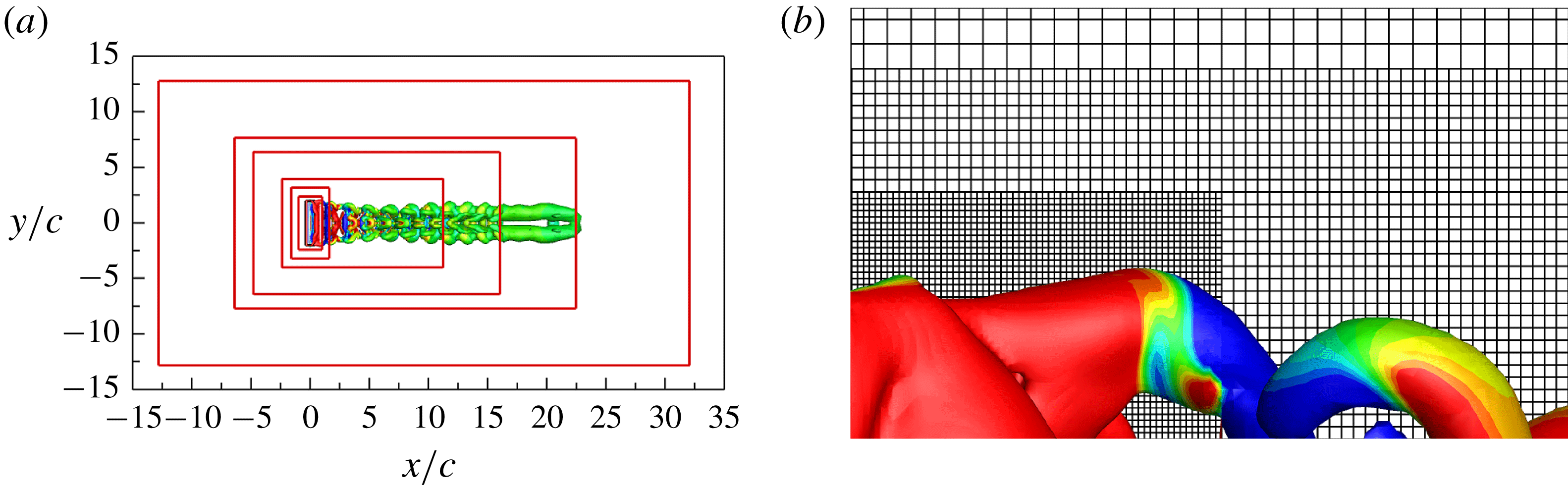
The computational domain with local mesh refinement: (a) boundaries of the six levels of refinement, top view; and (b) unstructured Cartesian mesh with hanging node, top view.

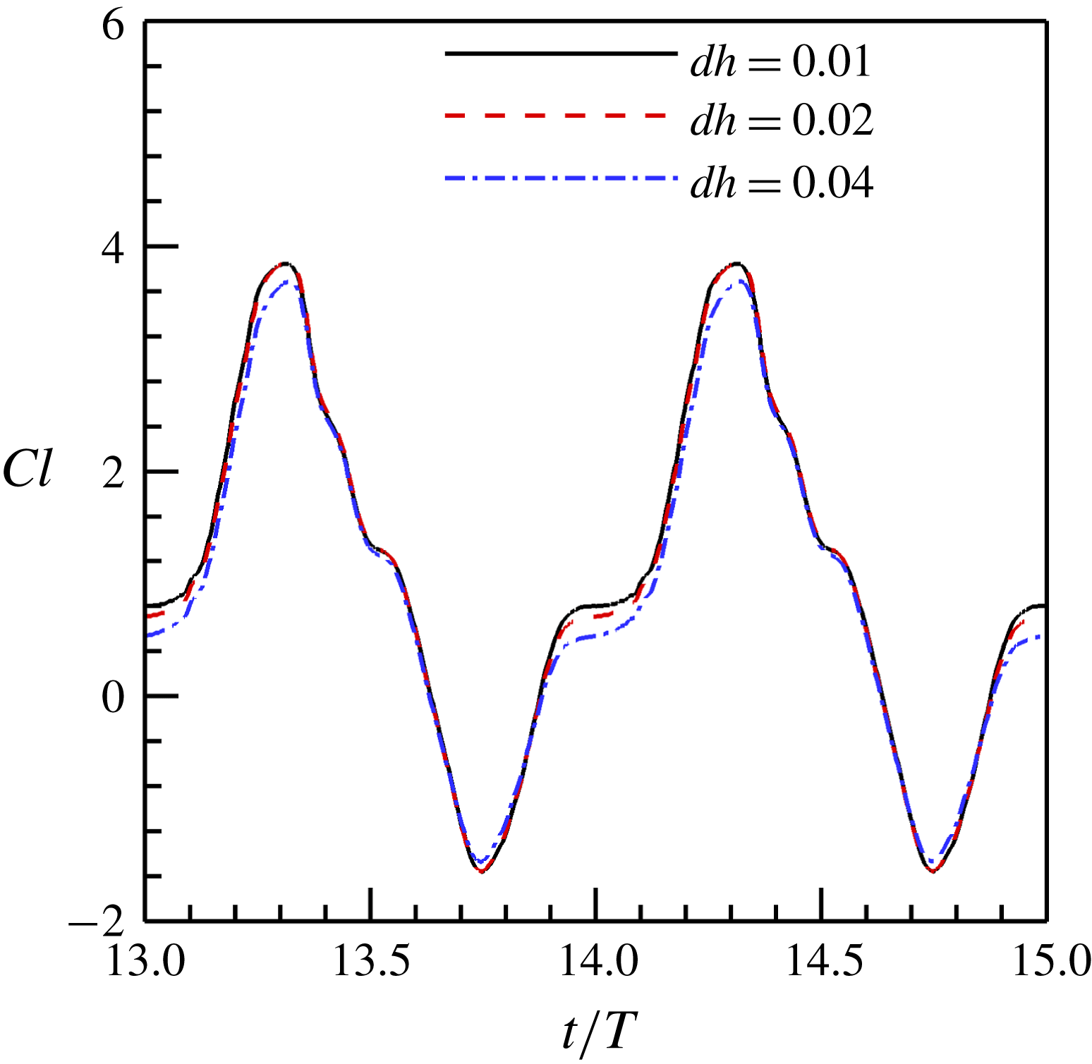
The time-dependent lift coefficients computed on different meshes in the case of the flapping wing with a fixed wingspan.

Appendix B. Numerical method and set-ups
Three different flapping wing models are considered to investigate the applicability of the KJ theorem in estimating the lift of flapping wings. The flows around the models are obtained by numerically solving the incompressible Navier–Stokes equations. The exact projection method is used to numerically decouple the velocity and pressure fields. A second-order finite volume method is used for the spatial discretization, and the three-step second-order Runge–Kutta method is used for the time integration. The moving boundary is dealt with by using an immersed boundary method. The details of the numerical method and the validations for different kinds of flows can be found in our previous work (Wang & Zhang Reference Wang and Zhang2011; Wang et al. Reference Wang, He and Zhang2013a ,Reference Wang, Zhang, He and Liu b ; Wang, He & Zhang Reference Wang, He and Zhang2015a ).
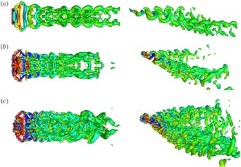
Typical wake structures of the flapping rectangular wing with a dynamically changing wingspan at three Strouhal numbers, (a)
 $St=0.3$
, (b)
 $St=0.6$
and (c)
 $St=0.9$
. The left and right columns show top and side views, respectively. The isosurfaces of
 $Q=0.2$
are shown. The colour shows the normalized spanwise vorticity from
 $-1$
(blue) to 1 (red).

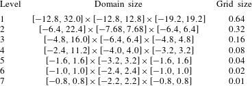
The simulations are conducted in a computational domain of
 $[-12.8c,32.0c]\times [-12.8c,12.8c]\times [-19.2c,19.2c]$
. The uniform upstream flow and free convection boundary conditions are specified at the inlet and outlet, respectively. The non-slip boundary condition is used on the wing surface. The slip boundary condition is set at other boundaries. The computational domain is discretized by using the unstructured Cartesian grid with up to seven levels of refinement. The schematic of the local refinement is shown in figure 24. The details of each level of refinement are listed in table 1. We simulated the case of flapping wing with a fixed wingspan on three different meshes. The three different meshes have seven, six and five levels of refinement, respectively. The minimum grid sizes of the three different meshes are
 $\text{d}h=0.01c$
,
 $\text{d}h=0.02c$
and
 $\text{d}h=0.04c$
, respectively. The time-dependent lift coefficients on the different meshes are shown in figure 25. The differences between the lift coefficients calculated at different levels decreases as the grid is refined. The simulation on a mesh with six levels of refinement (
 $\text{d}h=0.02c$
) gives almost the same lift coefficient as that on a finer mesh (
 $\text{d}h=0.01c$
). The maximum error of the lift coefficient on the mesh with six levels of refinement (
 $\text{d}h=0.02c$
) is within 1 % of the time-averaged lift coefficient (at
 $t/T=13.97$
as shown in figure 25). We simulate and present the results on the mesh with six levels of local refinement to balance the spatial resolution and computational cost. The total number of discretized cells on the mesh with six levels of local refinement is 5.18 million. The local refinement is also consistent with our previous simulations with the same or similar models (Wang et al.
Reference Wang, Zhang, He and Liu2013b
, Reference Wang, Zhang, He and Liu2015b
). The time step in the simulations is
 $0.005U/c$
, which corresponds to the maximum Courant–Friedrichs–Lewy number of approximately 0.5.
The time-averaged lift coefficient is denoted as
 $\langle Cl(t)\rangle$
, where
 $\langle \bullet \rangle =(1/T)\int _{0}^{T}\bullet \,\text{d}t$
is the time-averaged operator and
 $T$
is the flapping period. All the time-averaged variables in this work are computed based on equally sampled 20 datasets in one flapping period.
Boundaries and grid size of each level of refinement, normalized by using the chord length of the wing,
 $c$
.

The time-averaged lift coefficients at three Strouhal numbers, (a)
 $St=0.3$
, (b)
 $St=0.6$
and (c)
 $St=0.9$
based on simulations over 10 flapping periods, and (d)
 $St=0.9$
based on simulation simulations over 18 flapping periods.

The time-averaged lift coefficients estimated by using different models with different (a) Strouhal numbers, (b) time-averaged aspect ratios, (c) flapping amplitudes and (d) mean angles of attack. The solid symbols show the values estimated at three different Trefftz planes at
 $x/c=1.0$
,
 $x/c=1.5$
and
 $x/c=2.0$
.

The time-averaged vorticity-weighted wake width (VWW) as a function of the time-averaged circulation for the flapping wing with a dynamically changing wingspan at different parameters: (a) Strouhal numbers, (b) time-averaged aspect ratios, (c) flapping amplitudes, and (d) time-averaged angles of attack.

Appendix C. Parametric effects
Dimensionless parameters of the flapping wing with a dynamically changing wingspan.

The WS-KJ model is further evaluated in a parametric space consisting of the flapping frequency, span ratio (SR), aspect ratio, flapping amplitude and angle of attack for the flapping wing with a dynamically changing wingspan. The parameters in the simulations are given in table 2. We first investigated the flows at seven different Strouhal numbers ranging from 0.3 to 0.9 by adjusting the flapping frequency in (3.1) and (3.2), as the cases A1–A7 in table 2. The typical flow structures at
 $St=0.3$
, 0.6 and 0.9 are shown in figure 26. Similar to the observations reported in §§ 3–5, the LEV, TEV and TVs are generated by the flapping wing, which are advected downstream as they shed from the wing to form the complex wake structures. The advecting length scale of the flow structures in the near wake is given by the wake wavelength (Spedding et al.
Reference Spedding, Rosen and Hedenstrom2003)
 $\unicode[STIX]{x1D706}=U/f$
, where
 $U$
is the free-stream velocity and
 $f$
is the flapping frequency. As the Strouhal number increases, this wake wavelength describing the distance between the vortex rings decreases, resulting in increasingly complex wake structures due to the self- and mutually induced interactions of these structures, as shown in figure 26.
The time-averaged lift coefficients estimated by using different effective span lengths are shown in figure 27, which are consistent with those reported in §§ 3–5. The time-averaged lift coefficients computed based on the wingspan and DPV depend sensitively on the location of the Trefftz plane and deviate from the correct values. In contrast, the WS-KJ lift model is able to give the correct time-averaged lift coefficients for
 $x/\unicode[STIX]{x1D706}<10$
.
In the case of
 $St=0.9$
, the WS-KJ model gives the correct time-averaged lift coefficient as long as the Trefftz plane is located at
 $x/\unicode[STIX]{x1D706}<8$
. However, the estimated time-averaged lift coefficient starts to deviate from the correct value after
 $x/\unicode[STIX]{x1D706}=8$
. This deviation is caused by the vortex structures generated during the first two flapping periods where the effects of initial condition cannot be neglected, since the results in figure 27(a–c) are obtained in simulations conducted up to 10 flapping periods. To examine the initial effect, the flow is simulated up to 18 flapping periods, and as shown in figure 27(d). It is found that the WS-KJ model gives an improved time-averaged lift coefficient as long as the Trefftz plane is located at
 $x/\unicode[STIX]{x1D706}<10$
. The above results indicate that the WS-KJ model is applicable to the flapping flight at high Strouhal numbers up to 0.9 when the Trefftz plane is located in the near wake. For high Strouhal numbers, an alternative is to conduct simulations or measurements in a sufficiently long time span to minimize the effects of the vortex structures generated during the initial period. In the limiting case of very slow flight and hovering flight, the Strouhal number is very high, and the wake wavelength is very small. In this case, the Trefftz plane should be set to be very close to the wing trailing edge, and thus application of the WS-KJ model is difficult.
The time-averaged lift coefficients computed by using different effective span lengths are presented in figure 28. In all the cases in table 2, the WS-KJ model gives correct estimation of the time-averaged lift coefficients, while the results given by other models depend sensitively on the location of the Trefftz plane.
The VWW is evaluated based on the vorticity field in the Trefftz plane, and in general it is a complicated function of the location and time depending on the development of the wake vortex structures. Nevertheless, our numerical simulations indicate that the product of the time-averaged VWW and the time-averaged circulation (
 $\langle b_{vor}\rangle \langle \unicode[STIX]{x1D6E4}\rangle$
) remains constant at different locations for a given set of Strouhal number, aspect ratio, flapping amplitude and angle of attack (
 $AoA$
). This finding is consistent with our theoretical argument, i.e. the quantity
 $\langle b_{vor}\rangle \langle \unicode[STIX]{x1D6E4}\rangle$
is proportional to the lift of a wing according to (2.5). In this sense, this quantity is conserved for the given flapping parameters. Therefore,
 $\langle b_{vor}\rangle \langle \unicode[STIX]{x1D6E4}\rangle$
can be expressed as a function of the flapping parameters, i.e.
 $\langle b_{vor}\rangle \langle \unicode[STIX]{x1D6E4}\rangle =f(St,AR,A,\unicode[STIX]{x1D6FC}_{0})$
, where
 $St$
is the Strouhal number,
 $AR$
is the aspect ratio,
 $A$
is the heaving amplitude and
 $\unicode[STIX]{x1D6FC}_{0}$
is the mean
 $AoA$
. Figure 29 shows the time-averaged VWW as a function of the time-averaged circulation in log–log plots at different Strouhal numbers, time-averaged aspect ratios, flapping amplitudes and time-averaged angles of attack. The log–log plots indeed indicate the inversely proportional relationship between the time-averaged VWW and the time-averaged circulation at the different flapping parameters. These results further confirm the applicability of the WS-KJ model in a range of flapping parameters, providing a useful tool to understand the physics of unsteady lift generation.